LEARNING ON LARGE-SCALE TEXT-ATTRIBUTED GRAPHS VIA VARIATION AL INFERENCE
基于变分推理的大规模文本属性图学习
ABSTRACT
摘要
This paper studies learning on text-attributed graphs (TAGs), where each node is associated with a text description. An ideal solution for such a problem would be integrating both the text and graph structure information with large language models and graph neural networks (GNNs). However, the problem becomes very challenging when graphs are large due to the high computational complexity brought by training large language models and GNNs together. In this paper, we propose an efficient and effective solution to learning on large text-attributed graphs by fusing graph structure and language learning with a variation al ExpectationMaximization (EM) framework, called GLEM. Instead of simultaneously training large language models and GNNs on big graphs, GLEM proposes to alternatively update the two modules in the E-step and M-step. Such a procedure allows training the two modules separately while simultaneously allowing the two modules to interact and mutually enhance each other. Extensive experiments on multiple data sets demonstrate the efficiency and effectiveness of the proposed approach 1.
本文研究文本属性图(TAGs)上的学习问题,其中每个节点都与文本描述相关联。针对该问题的理想解决方案是将文本和图结构信息与大语言模型和图神经网络(GNNs)相整合。然而,当图规模较大时,由于同时训练大语言模型和GNNs带来的高计算复杂度,该问题变得极具挑战性。本文提出了一种高效且有效的解决方案GLEM,通过变分期望最大化(EM)框架融合图结构和语言学习来处理大规模文本属性图。GLEM没有选择在大图上同时训练大语言模型和GNNs,而是提出在E步和M步交替更新这两个模块。这种训练方式允许单独训练两个模块,同时使它们能够交互并相互增强。在多个数据集上的大量实验证明了所提方法的高效性和有效性[1]。
1 INTRODUCTION
1 引言
Graphs are ubiquitous in the real world. In many graphs, nodes are often associated with text attributes, resulting in text-attributed graphs (TAGs) (Yang et al., 2021). For example, in social graphs, each user might have a text description; in paper citation graphs, each paper is associated with its textual content. Learning on TAG has become an important research topic in multiple areas including graph learning, information retrieval, and natural language processing.
图在现实世界中无处不在。在许多图中,节点通常与文本属性相关联,从而形成文本属性图 (TAG) (Yang et al., 2021)。例如,在社交图中,每个用户可能有一段文本描述;在论文引用图中,每篇论文都与其文本内容相关联。TAG 学习已成为图学习、信息检索和自然语言处理等多个领域的重要研究课题。
In this paper, we focus on a fundamental problem, learning effective node representations, which could be used for a variety of applications such as node classification and link prediction. Intuitively, a TAG is rich in textual and structural information, both of which could be beneficial for learning good node representations. The textual information presents rich semantics to characterize the property of each node, and one could use a pre-trained language model (LM) (e.g., BERT (Devlin et al., 2019)) as a text encoder. Meanwhile, the structural information preserves the proximity between nodes, and connected nodes are more likely to have similar representations. Such structural relationships could be effectively modeled by a graph neural network (GNN) via the message-passing mechanism. In summary, LMs leverage the local textual information of individual nodes, while GNNs use the global structural relationship among nodes.
本文聚焦于一个基础性问题——学习有效的节点表征,该技术可应用于节点分类和链接预测等多种场景。直观来看,文本属性图(TAG)蕴含丰富的文本与结构信息,二者均有助于学习优质节点表征。其中,文本信息通过丰富语义刻画节点特性,可采用预训练语言模型(LM)(如BERT [20])作为文本编码器;而结构信息则维护节点间的邻近关系,相连节点往往具有相似表征。通过消息传递机制,图神经网络(GNN)能有效建模此类结构关系。总体而言,语言模型利用单个节点的局部文本信息,而图神经网络则利用节点间的全局结构关系。
An ideal approach for learning effective node representations is therefore to combine both the textual information and graph structure. One straightforward solution is to cascade an LM-based text encoder and GNN-based message-passing module and train both modules together. However, this method suffers from severe s cal ability issues. This is because the memory complexity is proportional to the graph size as neighborhood texts are also encoded. Therefore, on real-world TAGs where nodes are densely connected, the memory cost of this method would become un affordable.
因此,学习有效节点表征的理想方法是结合文本信息和图结构。一种直接的解决方案是将基于大语言模型的文本编码器和基于GNN的消息传递模块串联起来,并同时训练这两个模块。然而,这种方法存在严重的可扩展性问题,因为内存复杂度与图规模成正比(邻域文本也需要编码)。因此,在节点密集连接的真实世界TAG中,该方法的内存成本将变得难以承受。
To address such a problem, multiple solutions have been proposed. These methods reduce either the capacity of LMs or the size of graph structures for GNNs. More specifically, some studies choose to fix the parameters of LMs without fine-tuning them (Liu et al., 2020b). Some other studies reduce graph structures via edge sampling and perform message-passing only on the sampled edges (Zhu et al., 2021; Li et al., 2021a; Yang et al., 2021). Despite the improved s cal ability, reducing the LM capacity or graph size sacrifices the model effectiveness, leading to degraded performance of learning effective node representation. Therefore, we are wondering whether there exists a scalable and effective approach to integrating large LMs and GNNs on large text-attributed graphs.
为解决这一问题,已提出多种方案。这些方法要么降低大语言模型的容量,要么缩减图神经网络 (GNN) 的图结构规模。具体而言,部分研究选择固定大语言模型的参数而不进行微调 (Liu et al., 2020b) ,另一些研究则通过边采样简化图结构,仅在采样边上执行消息传递 (Zhu et al., 2021; Li et al., 2021a; Yang et al., 2021) 。尽管可扩展性有所提升,但降低模型容量或图规模会牺牲模型效能,导致学习有效节点表示的性能下降。因此,我们探索是否存在一种可扩展且高效的方法,能在大型文本属性图上集成大语言模型与图神经网络。
In this paper, we propose such an approach, named Graph and Language Learning by Expectation Maximization GLEM. In the GLEM, instead of simultaneously training both the LMs and GNNs, we leverage a variation al EM framework (Neal & Hinton, 1998) to alternatively update the two modules. Take the node classification task as an example. The LM uses local textual information of each node to learn a good representation for label prediction, which thus models label distributions conditioned on text attributes. By contrast, for a node, the GNN leverages the labels and textual encodings of surrounding nodes for label prediction, and it essentially defines a global conditional label distribution. The two components are optimized to maximize a variation al lower bound of the log-likelihood function, which can be achieved by alternating between an E-step and an M-step, where at each step we fix one component to update the other one. This separate training framework significantly improves the efficiency of GLEM, allowing it to scale up to real-world TAGs. In each step, one component presents pseudo-labels of nodes for the other component to mimic. By doing this, GLEM can effectively distill the local textual information and global structural information into both components, and thus GLEM enjoys better effectiveness in node classification. We conduct extensive experiments on three benchmark datasets to demonstrate the superior performance of GLEM. Notably, by leveraging the merits of both graph learning and language learning, GLEMLM achieves on par or even better performance than existing GNN models, GLEM-GNN achieves new state-of-the-art results on ogbn-arxiv, ogbn-product, and ogbn-papers100M.
本文提出了一种名为图与语言期望最大化学习 (Graph and Language Learning by Expectation Maximization, GLEM) 的方法。在GLEM中,我们采用变分EM框架 (Neal & Hinton, 1998) 交替更新语言模型和图神经网络模块,而非同时训练二者。以节点分类任务为例:语言模型利用各节点的局部文本信息学习标签预测的优质表征,从而建模基于文本属性的标签条件分布;而图神经网络则通过邻域节点的标签与文本编码进行预测,本质上定义了全局标签条件分布。通过交替执行E步和M步(固定一个模块更新另一个模块),这两个组件被优化以最大化对数似然函数的变分下界。这种分离式训练框架显著提升了GLEM的效率,使其能够扩展到现实世界的异质信息网络。在每轮迭代中,一个组件会生成供另一个组件学习的节点伪标签。通过这种方式,GLEM能有效将局部文本信息与全局结构信息蒸馏至两个组件,从而获得更优的节点分类性能。我们在三个基准数据集上的实验表明:融合图学习与语言学习优势的GLEM-LM性能媲美甚至超越现有图神经网络,GLEM-GNN则在ogbn-arxiv、ogbn-product和ogbn-papers100M数据集上创造了最新最优结果。
2 RELATED WORK
2 相关工作
Representation learning on text-attributed graphs (TAGs) (Yang et al., 2021) has been attracting growing attention in graph machine learning, and one of the most important problems is node classification. The problem can be directly formalized as a text representation learning task, where the goal is to use the text feature of each node for learning. Early works resort to convolutional neural networks (Kim, 2014; Shen et al., 2014) or recurrent neural networks Tai et al. (2015). Recently, with the superior performance of transformers (Vaswani et al., 2017) and pre-trained language models (Devlin et al., 2019; Yang et al., 2019), LMs have become the go-to model for encoding contextual semantics in sentences for text representation learning. At the same time, the problem can also be viewed as a graph learning task that has been vastly developed by graph neural networks (GNNs) (Kipf & Welling, 2017; Velickovic et al., 2018; Xu et al., 2019; Zhang & Chen, 2018; Teru et al., 2020). A GNN takes numerical features as input and learns node representations by transforming representations and aggregating them according to the graph structure. With the capability of considering both node attributes and graph structures, GNNs have shown great performance in various applications, including node classification and link prediction. Nevertheless, LMs and GNNs only focus on parts of observed information (i.e., textual or structural) for representation learning, and the results remain to be improved.
文本属性图(TAGs)上的表示学习(Yang等人,2021)在图机器学习中日益受到关注,其中最重要的问题之一是节点分类。该问题可直接形式化为文本表示学习任务,目标是利用每个节点的文本特征进行学习。早期研究采用卷积神经网络(Kim,2014;Shen等人,2014)或循环神经网络(Tai等人,2015)。近年来,随着Transformer(Vaswani等人,2017)和预训练语言模型(Devlin等人,2019;Yang等人,2019)的卓越表现,大语言模型已成为文本表示学习中编码句子上下文语义的首选模型。同时,该问题也可视为图学习任务,由图神经网络(GNNs)(Kipf & Welling,2017;Velickovic等人,2018;Xu等人,2019;Zhang & Chen,2018;Teru等人,2020)广泛发展。GNN以数值特征为输入,通过转换表示并根据图结构聚合来学习节点表示。由于能同时考虑节点属性和图结构,GNN在节点分类和链接预测等应用中表现出色。然而,大语言模型和GNN仅关注部分观测信息(即文本或结构)进行表示学习,结果仍有改进空间。
There are some recent efforts focusing on the combination of GNNs and LMs, which allows one to enjoy the merits of both models. One widely adopted way is to encode the texts of nodes with a fixed LM, and further treat the LM embeddings as features to train a GNN for message passing. Recently, a few methods propose to utilize domain-adaptive pre training (Gururangan et al., 2020) on TAGs and predict the graph structure using LMs (Chien et al., 2022; Yasunaga et al., 2022) to provide better LM embeddings for GNN. Despite better results, these LM embeddings still remain unlearn able in the GNN training phase. Such a separated training paradigm ensures the model s cal ability as the number of trainable parameters in GNNs is relatively small. However, its performance is hindered by the task and topology-irrelevant semantic modeling process. To overcome these limitations, endeavors have been made (Zhu et al., 2021; Li et al., 2021a; Yang et al., 2021; Bi et al., 2021; Pang et al., 2022) to co-train GNNs and LM under a joint learning framework. However, such co-training approaches suffer from severe s cal ability issues as all the neighbors need to be encoded by language models from scratch, incurring huge extra computation costs. In practice, these models restrict the message-passing to very few, e.g. 3 (Li et al., 2021a; Zhu et al., 2021), sampled first-hop neighbors, resulting in severe information loss.
近期有一些研究致力于将图神经网络 (GNN) 与大语言模型 (LM) 相结合,以同时发挥两种模型的优势。一种广泛采用的方法是使用固定的大语言模型对节点文本进行编码,并将这些语言模型嵌入作为特征来训练用于消息传递的图神经网络。最近,部分方法提出在文本属性图 (TAG) 上进行领域自适应预训练 (Gururangan et al., 2020),并利用大语言模型预测图结构 (Chien et al., 2022; Yasunaga et al., 2022),从而为图神经网络提供更好的语言模型嵌入。尽管效果有所提升,但这些语言模型嵌入在图神经网络训练阶段仍无法被学习。这种分离的训练范式通过保持图神经网络中可训练参数数量较少来确保模型的可扩展性,但其性能受限于与任务及拓扑无关的语义建模过程。
为突破这些限制,研究者们 (Zhu et al., 2021; Li et al., 2021a; Yang et al., 2021; Bi et al., 2021; Pang et al., 2022) 尝试在联合学习框架下对图神经网络和大语言模型进行协同训练。然而,此类协同训练方法面临严重的可扩展性问题——由于所有邻居节点都需要通过语言模型从头开始编码,导致巨大的额外计算开销。实践中,这些模型将消息传递限制在极少数(例如3个 (Li et al., 2021a; Zhu et al., 2021))采样的一跳邻居节点,造成严重的信息损失。
To summarize, existing methods of fusing LMs and GNNs suffer from either unsatisfactory results or poor s cal ability. In contrast to these methods, GLEM uses a pseudo-likelihood variation al framework to integrate an LM and a GNN, which allows the two components to be trained separately, leading to good s cal ability. Also, GLEM encourages the collaboration of both components, so that it is able to use both textual semantics and structural semantics for representation learning, and thus enjoys better effectiveness.
综上所述,现有融合大语言模型(LM)和图神经网络(GNN)的方法要么效果欠佳,要么扩展性不足。与这些方法不同,GLEM采用伪似然变分框架来集成LM和GNN,使两个组件能够分别训练,从而具备良好的扩展性。同时,GLEM促进两个组件的协同合作,使其能够同时利用文本语义和结构语义进行表征学习,因此具有更好的效果。
Besides, there are also some efforts using GNNs for text classification. Different from our approach, which uses GNNs to model the observed structural relationship between nodes, these methods assume graph structures are unobserved. They apply GNNs on synthetic graphs generated by words in a text (Huang et al., 2019; Hu et al., 2019; Zhang et al., 2020) or co-occurrence patterns between texts and words (Huang et al., 2019; Liu et al., 2020a). As structures are observed in the problem of node classification in text-attributed graphs, these methods cannot well address the studied problem.
此外,也有一些研究尝试用图神经网络 (GNN) 进行文本分类。与我们的方法不同(即用 GNN 建模节点间已观测到的结构关系),这些方法假设图结构未被观测到。它们将 GNN 应用于由文本中的单词生成的合成图 (Huang et al., 2019; Hu et al., 2019; Zhang et al., 2020) 或文本与单词间的共现模式 (Huang et al., 2019; Liu et al., 2020a)。由于文本属性图中的节点分类问题存在可观测结构,这些方法无法有效解决我们所研究的问题。
Lastly, our work is related to GMNN Qu et al. (2019), which also uses a pseudo-likelihood variational framework for node representation learning. However, GMNN aims to combine two GNNs for general graphs and it does not consider modeling textual features. Different from GMNN, GLEM focuses on TAGs, which are more challenging to deal with. Also, GLEM fuses a GNN and an LM, which can better leverage both structural features and textual features in a TAG, and thus achieves state-of-the-art results on a few benchmarks.
最后,我们的工作与GMNN [Qu等人,2019]相关,后者同样采用伪似然变分框架进行节点表示学习。然而,GMNN旨在为通用图结合两种GNN,并未考虑文本特征建模。与GMNN不同,GLEM专注于更具挑战性的TAG(文本属性图),并通过融合GNN和LM(语言模型)更有效地利用TAG中的结构特征与文本特征,从而在多个基准测试中取得最先进的结果。
3 BACKGROUND
3 背景
In this paper, we focus on learning representations for nodes in TAGs, where we take node classification as an example for illustration. Before diving into the details of our proposed GLEM, we start with presenting a few basic concepts, including the definition of TAGs and how LMs and GNNs can be used for node classification in TAGs.
本文重点研究时序属性图(TAG)中的节点表征学习,并以节点分类任务为例进行说明。在详细介绍我们提出的GLEM方法之前,首先介绍几个基本概念,包括TAG的定义以及如何利用大语言模型和图神经网络在TAG中实现节点分类。
3.1 TEXT-ATTRIBUTED GRAPH
3.1 文本属性图 (Text-Attributed Graph)
Formally, a TAG ${\mathcal G}{S}=~\left(V,A,{\bf s}{V}\right)$ is composed of nodes $V$ and their adjacency matrix $A\in$ $\mathbb{R}^{|V|\times|\bar{V}|}$ , where each node $n\in V$ is associated with a sequential text feature (sentence) ${\bf s}{n}$ . In this paper, we study the problem of node classification on TAGs. Given a few labeled nodes $\mathbf{y}{L}$ of $L\subset V$ , the goal is to predict the labels $\mathbf{y}_{U}$ for the remaining unlabeled objects $U=V\setminus L$ .
形式上,一个TAG ${\mathcal G}{S}=~\left(V,A,{\bf s}{V}\right)$ 由节点 $V$ 及其邻接矩阵 $A\in$ $\mathbb{R}^{|V|\times|\bar{V}|}$ 组成,其中每个节点 $n\in V$ 关联一个序列文本特征(句子) ${\bf s}{n}$。本文研究TAG上的节点分类问题:给定少量已标注节点 $\mathbf{y}{L}$ (其中 $L\subset V$),目标是预测剩余未标注对象 $U=V\setminus L$ 的标签 $\mathbf{y}_{U}$。
Intuitively, node labels can be predicted by using either the textual information or the structural information, and representative methods are language models (LMs) and graph neural networks (GNNs) respectively. Next, we introduce the high-level ideas of both methods.
直观来看,节点标签既可通过文本信息也可通过结构信息进行预测,其代表性方法分别是大语言模型 (LMs) 和图神经网络 (GNNs)。接下来我们将介绍这两种方法的核心思想。
3.2 LANGUAGE MODELS FOR NODE CLASSIFICATION
3.2 用于节点分类的语言模型
Language models aim to use the sentence ${\bf s}_{n}$ of each node $n$ for label prediction, resulting in a text classification task (Socher et al., 2013; Williams et al., 2018). The workflow of LMs can be characterized as below:
语言模型旨在利用每个节点$n$的句子${\bf s}_{n}$进行标签预测,从而形成文本分类任务 (Socher et al., 2013; Williams et al., 2018)。其工作流程可描述如下:
$$
p_{\theta}(\mathbf{y}{n}|\mathbf{s}{n})=\mathrm{Cat}(\mathbf{y}{n}\mid\mathrm{softmax}(\mathrm{MLP}{\theta_{2}}(\mathbf{h}{n})));\qquad\mathbf{h}{n}=\mathrm{SeqEnc}{\theta_{1}}(\mathbf{s}_{n}),
$$
$$
p_{\theta}(\mathbf{y}{n}|\mathbf{s}{n})=\mathrm{Cat}(\mathbf{y}{n}\mid\mathrm{softmax}(\mathrm{MLP}{\theta_{2}}(\mathbf{h}{n})));\qquad\mathbf{h}{n}=\mathrm{SeqEnc}{\theta_{1}}(\mathbf{s}_{n}),
$$
where $\mathrm{SeqEnc}{\theta_{1}}$ is a text encoder such as a transformer-based model (Vaswani et al., 2017; Yang et al., 2019), which projects the sentence ${\bf s}{n}$ into a vector representation $\mathbf{h}{n}$ . Afterwards, the node label distribution ${\mathbf y}{n}$ can be simply predicted by applying an $\mathrm{MLP}{\theta_{2}}$ with a softmax function to ${\bf h}_{n}$ .
其中 $\mathrm{SeqEnc}{\theta_{1}}$ 是基于Transformer的文本编码器 (Vaswani et al., 2017; Yang et al., 2019),它将句子 ${\bf s}{n}$ 映射为向量表示 $\mathbf{h}{n}$。随后,通过将 $\mathrm{MLP}{\theta_{2}}$ 和softmax函数应用于 ${\bf h}{n}$,即可简单预测节点标签分布 ${\mathbf y}_{n}$。
Leveraging deep architectures and pre-training on large-scale corpora, LMs achieve impressive results on many text classification tasks (Devlin et al., 2019; Liu et al., 2019). Nevertheless, the memory cost is often high due to large model sizes. Also, for each node, LMs solely use its own sentence for classification, and the interactions between nodes are ignored, leading to sub-optimal results especially on nodes with insufficient text features.
借助深度架构和大规模语料库的预训练,大语言模型 (LLM) 在许多文本分类任务中取得了令人瞩目的成果 (Devlin et al., 2019; Liu et al., 2019)。然而,由于模型规模庞大,内存消耗往往很高。此外,对于每个节点,大语言模型仅使用其自身的句子进行分类,而忽略了节点之间的交互,这导致结果欠佳,尤其是在文本特征不足的节点上。
3.3 GRAPH NEURAL NETWORKS FOR NODE CLASSIFICATION
3.3 用于节点分类的图神经网络
Graph neural networks approach node classification by using the structural interactions between nodes. Specifically, GNNs leverage a message-passing mechanism, which can be described as:
图神经网络 (Graph Neural Networks) 通过利用节点间的结构交互关系进行节点分类。具体而言,GNN采用消息传递机制,其过程可描述为:
$$
\begin{array}{r}{p_{\phi}(\mathbf{y}{n}|A)=\mathrm{Cat}(\mathbf{y}{n}|\mathrm{softmax}(\mathbf{h}{n}^{(L)}));\qquad\mathbf{h}{n}^{(l)}=\sigma(\mathrm{AGG}{\phi}(\mathrm{MSG}{\phi}(\mathbf{h}_{\mathrm{NB}(n)}^{(l-1)}),A)),}\end{array}
$$
$$
\begin{array}{r}{p_{\phi}(\mathbf{y}{n}|A)=\mathrm{Cat}(\mathbf{y}{n}|\mathrm{softmax}(\mathbf{h}{n}^{(L)}));\qquad\mathbf{h}{n}^{(l)}=\sigma(\mathrm{AGG}{\phi}(\mathrm{MSG}{\phi}(\mathbf{h}_{\mathrm{NB}(n)}^{(l-1)}),A)),}\end{array}
$$
where $\phi$ denotes the parameters of GNN, $\sigma$ is an activation function, $\mathrm{MSG}{\phi}(\cdot)$ and $\mathrm{AGG}{\phi}(\cdot)$ stand for the message and aggregation functions respectively, $\mathrm{NB}(n)$ denotes the neighbor nodes of $n$ . Given the initial text encodings $\mathbf{h}_{n}^{(0)}$ , e.g. pre-trained LM embeddings, a GNN iterative ly updates them by applying the message function and the aggregation function, so that the learned node represent at ions and predictions can well capture the structural interactions between nodes.
其中 $\phi$ 表示 GNN 的参数,$\sigma$ 是激活函数,$\mathrm{MSG}{\phi}(\cdot)$ 和 $\mathrm{AGG}{\phi}(\cdot)$ 分别表示消息函数和聚合函数,$\mathrm{NB}(n)$ 表示节点 $n$ 的邻居节点。给定初始文本编码 $\mathbf{h}_{n}^{(0)}$(例如预训练语言模型嵌入向量),GNN 通过迭代应用消息函数和聚合函数来更新这些编码,使得学习到的节点表示和预测能够充分捕捉节点间的结构交互关系。
With the message-passing mechanism, GNNs are able to effectively leverage the structural information for node classification. Despite the good performance on many graphs, GNNs are not able to well utilize the textual information, and thus GNNs often suffer on nodes with few neighbors.
借助消息传递机制,图神经网络(GNN)能够有效利用结构信息进行节点分类。尽管在许多图数据上表现良好,GNN仍难以充分利用文本信息,因此在邻居节点较少的场景下往往表现不佳。
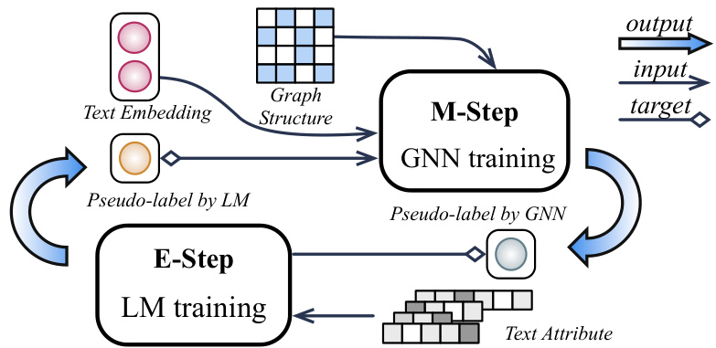
Figure 1: The proposed GLEM framework trains GNN and LM separately in a variation al EM framework: In E-step, an LM is trained towards predicting both the gold labels and GNN-predicted pseudo-labels; In M-step, a GNN is trained by predicting both gold labels and LM-inferred pseudolabels using the embeddings and pseudo-labels predicted by LM.
图 1: 提出的GLEM框架在变分EM框架中分别训练GNN和LM:在E步中,LM被训练用于预测真实标签和GNN预测的伪标签;在M步中,GNN通过预测真实标签和LM推断的伪标签进行训练,同时使用LM生成的嵌入和伪标签。
4 METHODOLOGY
4 方法论
In this section, we introduce our proposed approach which combines GNN and LM for node represent ation learning in TAGs. Existing methods either suffer from s cal ability issues or have poor results in downstream applications such as node classification. Therefore, we are looking for an approach that enjoys both good s cal ability and capacity.
在本节中,我们介绍结合图神经网络(GNN)与大语言模型(LM)的TAG节点表征学习方法。现有方法要么存在可扩展性问题,要么在节点分类等下游任务中表现欠佳。因此,我们寻求兼具良好可扩展性与表征能力的新方法。
Toward this goal, we take node classification as an example and propose GLEM. GLEM leverages a variation al EM framework, where the LM uses the text information of each sole node to predict its label, which essentially models the label distribution conditioned on local text attribute; whereas the GNN leverages the text and label information of surrounding nodes for label prediction, which characterizes the global conditional label distribution. The two modules are optimized by alternating between an E-step and an M-step. In the E-step, we fix the GNN and let the LM mimic the labels inferred by the GNN, allowing the global knowledge learned by the GNN to be distilled into the LM. In the M-step, we fix the LM, and the GNN is optimized by using the node representations learned by the LM as features and the node labels inferred by the LM as targets. By doing this, the GNN can effectively capture the global correlations of nodes for precise label prediction. With such a framework, the LM and GNN can be trained separately, leading to better s cal ability. Meanwhile, the LM and GNN are encouraged to benefit each other, without sacrificing model performance.
为实现这一目标,我们以节点分类为例提出了GLEM。GLEM采用变分EM框架:大语言模型利用单个节点的文本信息预测其标签,本质上是建模基于局部文本属性的标签分布;而图神经网络则利用周围节点的文本和标签信息进行预测,刻画全局条件标签分布。两个模块通过交替执行E步和M步进行优化:
- E步:固定图神经网络,让大语言模型模仿其推断的标签,使图神经网络习得的全局知识蒸馏至语言模型中;
- M步:固定语言模型,以语言模型学习的节点表征作为特征、其推断的节点标签作为目标来优化图神经网络,从而有效捕捉节点的全局相关性以实现精准预测。
该框架支持语言模型与图神经网络分别训练,具备更强可扩展性。同时两者能相互促进,且不牺牲模型性能。
4.1 THE PSEUDO-LIKELIHOOD VARIATION AL FRAMEWORK
4.1 伪似然变分AL框架
Our approach is based on a pseudo-likelihood variation al framework, which offers a principled and flexible formalization for model design. To be more specific, the framework tries to maximize the log-likelihood function of the observed node labels, i.e., $p(\mathbf{y}{L}|\mathbf{s}{V},A)$ . Directly optimizing the function is often hard due to the unobserved node labels $\mathbf{y}_{U}$ , and thus the framework instead optimizes the evidence lower bound as below:
我们的方法基于一种伪似然变分框架,该框架为模型设计提供了原则性且灵活的形式化表达。具体而言,该框架试图最大化观测节点标签的对数似然函数,即 $p(\mathbf{y}{L}|\mathbf{s}{V},A)$ 。由于未观测节点标签 $\mathbf{y}_{U}$ 的存在,直接优化该函数通常较为困难,因此框架转而优化如下证据下界:
$$
\begin{array}{r}{\log p\big(\mathbf{y}{L}\vert\mathbf{s}{V},A\big)\geq\mathbb{E}{q(\mathbf{y}{U}\vert\mathbf{s}{U})}\bigl[\log p\big(\mathbf{y}{L},\mathbf{y}{U}\vert\mathbf{s}{V},A\big)-\log q(\mathbf{y}{U}\vert\mathbf{s}_{U})\bigr],}\end{array}
$$
where $q(\mathbf{y}{U}|\mathbf{s}_{U})$ is a variation al distribution and the above inequality holds for any $q$ . The ELBO can be optimized by alternating between optimizing the distribution $q$ (i.e., $\mathrm{E}$ -step) and the distribution $p$
其中 $q(\mathbf{y}{U}|\mathbf{s}_{U})$ 是一个变分分布,且上述不等式对任意 $q$ 都成立。可以通过交替优化分布 $q$ (即 $\mathrm{E}$ 步) 和分布 $p$ 来优化ELBO。
(i.e., M-step). In the $\mathrm{E}$ -step, we aim at updating $q$ to minimize the KL divergence between $q(\mathbf{y}{U}|\mathbf{s}{U})$ and $p(\mathbf{y}{U}|\mathbf{s}{V},A,\mathbf{y}_{L})$ , so that the above lower bound can be tightened. In the M-step, we then update $p$ towards maximizing the following pseudo-likelihood (Besag, 1975) function:
(i.e., M-step). 在 $\mathrm{E}$ 步中,我们的目标是更新 $q$ 以最小化 $q(\mathbf{y}{U}|\mathbf{s}{U})$ 和 $p(\mathbf{y}{U}|\mathbf{s}{V},A,\mathbf{y}_{L})$ 之间的 KL 散度,从而收紧上述下界。在 M 步中,我们更新 $p$ 以最大化以下伪似然 (Besag, 1975) 函数:
$$
{\mathbb E}{q({\mathbf{y}}{U}\mid{\mathbf{s}}{U})}[\log p({\mathbf{y}}{L},{\mathbf{y}}{U}\mid{\mathbf{s}}{V},A)]\approx{\mathbb E}{q({\mathbf{y}}{U}\mid{\mathbf{s}}{U})}[\sum_{n\in V}\log p({\mathbf{y}}{n}|{\mathbf{s}}{V},A,{\mathbf{y}}_{V\setminus n})].
$$
The pseudo-likelihood variation al framework yields a formalization with two distributions to maximize data likelihood. The two distributions are trained via a separate $\mathrm{E}$ -step and M-step, and thus we no longer need the end-to-end training paradigm, leading to better s cal ability which naturally fits our scenario. Next, we introduce how we apply the framework to node classification in TAGs by instant i a ting the $p$ and $q$ distributions with GNNs and LMs respectively.
伪似然变分框架通过最大化数据似然性的两个分布实现了形式化。这两个分布通过独立的$\mathrm{E}$步和M步进行训练,因此我们不再需要端到端训练范式,从而获得更好的可扩展性,这自然契合我们的场景。接着,我们将介绍如何通过分别用GNN和LM实例化$p$与$q$分布,将该框架应用于TAG中的节点分类任务。
4.2 PARAMETER IZ ATION
4.2 参数化
The distribution $q$ aims to use the text information $\mathbf{s}_{U}$ to define node label distribution. In GLEM, we use a mean-field form, assuming the labels of different nodes are independent and the label of each node only depends on its own text information, yielding the following form of factorization:
分布 $q$ 旨在利用文本信息 $\mathbf{s}_{U}$ 定义节点标签分布。在GLEM中,我们采用平均场形式,假设不同节点的标签相互独立,且每个节点的标签仅取决于其自身的文本信息,从而得到以下因子分解形式:
$$
q_{\theta}(\mathbf{y}{U}|\mathbf{s}{U})=\prod_{n\in U}q_{\theta}(\mathbf{y}{n}|\mathbf{s}_{n}).
$$
As introduced in Section 3.2, each term $q_{\theta}(\mathbf{y}{n}|\mathbf{s}{n})$ can be modeled by a transformer-based LM $q_{\theta}$ parameterized by $\theta$ , which effectively models the fine-grained token interactions by the attention mechanism (Vaswani et al., 2017).
如第3.2节所述,每个项$q_{\theta}(\mathbf{y}{n}|\mathbf{s}{n})$可通过基于Transformer的语言模型$q_{\theta}$建模,该模型由参数$\theta$定义,并利用注意力机制 (Vaswani et al., 2017) 有效捕捉细粒度token间的交互关系。
On the other hand, the distribution $p$ defines a conditional distribution $p_{\phi}(\mathbf{y}{n}|\mathbf{s}{V},A,\mathbf{y}{V\setminus n}),$ , aiming to leverage the node features $\mathbf{s}{V}$ , graph structure $A$ , and other node labels $\mathbf{y}{V\setminus n}$ to characterize the label distribution of each node $n$ . Such a formalization can be naturally captured by a GNN through the message-passing mechanism. Thus, we model $p_{\phi}(\mathbf{y}{n}|\mathbf{s}{V},A,\mathbf{y}{V\setminus n})$ as a $\mathrm{GNN}p_{\phi}$ parameterized by $\phi$ to effectively model the structural interactions between nodes. Note that the $\mathrm{GNN}p_{\phi}$ takes the node texts $\mathbf{s}{V}$ as input to output the node label distribution. However, the node texts are discrete variables, which cannot be directly used by the GNN. Thus, in practice we first encode the node texts with the LM $q_{\theta}$ , and then use the obtained embeddings as a surrogate of node texts for the GNN pφ.
另一方面,分布 $p$ 定义了一个条件分布 $p_{\phi}(\mathbf{y}{n}|\mathbf{s}{V},A,\mathbf{y}{V\setminus n})$,旨在利用节点特征 $\mathbf{s}{V}$、图结构 $A$ 和其他节点标签 $\mathbf{y}{V\setminus n}$ 来表征每个节点 $n$ 的标签分布。这种形式化可以通过 GNN 的消息传递机制自然捕获。因此,我们将 $p_{\phi}(\mathbf{y}{n}|\mathbf{s}{V},A,\mathbf{y}{V\setminus n})$ 建模为由 $\phi$ 参数化的 $\mathrm{GNN}p_{\phi}$,以有效建模节点间的结构交互。需要注意的是,$\mathrm{GNN}p_{\phi}$ 以节点文本 $\mathbf{s}{V}$ 作为输入来输出节点标签分布。然而,节点文本是离散变量,无法直接被 GNN 使用。因此,实践中我们首先用大语言模型 $q_{\theta}$ 对节点文本进行编码,然后将获得的嵌入作为节点文本的替代用于 GNN pφ。
In the following sections, we further explain how we optimize the LM $q_{\theta}$ and the GNN $p_{\phi}$ to let them collaborate with each other.
在以下章节中,我们将进一步阐述如何优化语言模型 $q_{\theta}$ 和图神经网络 $p_{\phi}$,使它们能够相互协作。
4.3 E-STEP: LM OPTIMIZATION
4.3 E-STEP: 语言模型优化
In the E-step, we fix the GNN and aim to update the LM to maximize the evidence lower bound. By doing this, the global semantic correlations between different nodes can be distilled into the LM.
在E步中,我们固定GNN并更新LM以最大化证据下界。通过这一步骤,不同节点间的全局语义关联可被蒸馏至LM中。
Formally, maximizing the evidence lower bound with respect to the LM is equivalent to minimizing the KL divergence between the posterior distribution and the variation al distribution, i.e., $\begin{array}{r}{\mathrm{KL}(q_{\theta}(\mathbf{y}{U}|\mathbf{s}{U})||p_{\phi}(\mathbf{y}{U}|\mathbf{s}{V},A,\mathbf{y}{L}))}\end{array}$ . However, directly optimizing the KL divergence is nontrivial, as the KL divergence relies on the entropy of $q_{\theta}(\mathbf{y}{U}|\mathbf{s}{U})$ , which is hard to deal with. To overcome the challenge, we follow the wake-sleep algorithm (Hinton et al., 1995) to minimize the reverse KL divergence, yielding the following objective function to maximize with respect to the $\operatorname{LM}q_{\theta}$ :
形式上,最大化证据下界 (evidence lower bound) 关于大语言模型的优化等价于最小化后验分布与变分分布之间的KL散度 (KL divergence) ,即 $\begin{array}{r}{\mathrm{KL}(q_{\theta}(\mathbf{y}{U}|\mathbf{s}{U})||p_{\phi}(\mathbf{y}{U}|\mathbf{s}{V},A,\mathbf{y}{L}))}\end{array}$ 。然而直接优化KL散度并非易事,因为KL散度依赖于 $q_{\theta}(\mathbf{y}{U}|\mathbf{s}{U})$ 的熵,这一项难以处理。为克服该挑战,我们采用唤醒-睡眠算法 (wake-sleep algorithm) [Hinton et al., 1995] 来最小化反向KL散度,从而得到关于 $\operatorname{LM}q_{\theta}$ 的最大化目标函数:
$$
\begin{array}{r l}&{-{\mathrm{KL}}\displaystyle(p_{\phi}(\mathbf{y}{U}\vert\mathbf{s}{V},A,\mathbf{y}{L})\vert\vert q_{\theta}(\mathbf{y}{U}\vert\mathbf{s}{U}))=\mathbb{E}{p_{\phi}(\mathbf{y}{U}\vert\mathbf{s}{V},A,\mathbf{y}{L})}\big[\log q_{\theta}(\mathbf{y}{U}\vert\mathbf{s}{U})\big]+\mathrm{const}}\ &{\quad\quad\quad\quad=\displaystyle\sum_{n\in U}\mathbb{E}{p_{\phi}(\mathbf{y}{n}\vert\mathbf{s}{V},A,\mathbf{y}{L})}\big[\log q_{\theta}(\mathbf{y}{n}\vert\mathbf{s}_{n})\big]+\mathrm{const},}\end{array}
$$
which is more tractable as we no longer need to consider the entropy of $q_{\theta}(\mathbf{y}{U}|\mathbf{s}{U})$ . Now, the sole difficulty lies in computing the distribution $p_{\phi}(\mathbf{y}{n}|\mathbf{s}{V},A,\mathbf{y}{L})$ . Remember that in the original GNN which defines the distribution $p_{\phi}(\mathbf{y}{n}|\mathbf{s}{V},A,\mathbf{y}{V\setminus n})$ , we aim to predict the label distribution of a node $n$ based on the surrounding node labels $\mathbf{y}{V\setminus n}$ . However, in the above distribution $p_{\phi}(\mathbf{y}{n}|\mathbf{s}{V},A,\mathbf{y}{L})$ , we only condition on the observed node labels $\mathbf{y}_{L}$ , and the labels of other nodes are unspecified, so we cannot compute the distribution directly with the GNN. In order to solve the problem, we propose to annotate all the unlabeled nodes in the graph with the pseudo-labels predicted by the LM, so that we can approximate the distribution as follows:
这变得更加易于处理,因为我们不再需要考虑 $q_{\theta}(\mathbf{y}{U}|\mathbf{s}{U})$ 的熵。现在,唯一的困难在于计算分布 $p_{\phi}(\mathbf{y}{n}|\mathbf{s}{V},A,\mathbf{y}{L})$ 。请注意,在原始定义分布 $p_{\phi}(\mathbf{y}{n}|\mathbf{s}{V},A,\mathbf{y}{V\setminus n})$ 的 GNN 中,我们的目标是根据周围节点标签 $\mathbf{y}{V\setminus n}$ 预测节点 $n$ 的标签分布。然而,在上述分布 $p_{\phi}(\mathbf{y}{n}|\mathbf{s}{V},A,\mathbf{y}{L})$ 中,我们仅以观测到的节点标签 $\mathbf{y}_{L}$ 为条件,其他节点的标签未指定,因此无法直接通过 GNN 计算该分布。为了解决这个问题,我们建议用大语言模型预测的伪标签标注图中所有未标记节点,从而可以按如下方式近似该分布:
$$
p_{\phi}(\mathbf{y}{n}|\mathbf{s}{V},A,\mathbf{y}{L})\approx p_{\phi}(\mathbf{y}{n}|\mathbf{s}{V},A,\mathbf{y}{L},\hat{\mathbf{y}}_{U\setminus n}),
$$
where $\hat{\mathbf{y}}{U\backslash n}={\hat{\mathbf{y}}{n^{\prime}}}{n^{\prime}\in U\backslash n}$ with each $\hat{\mathbf{y}}{n^{\prime}}\sim q_{\theta}(\mathbf{y}{n^{\prime}}|\mathbf{s}_{n^{\prime}})$ .
其中 $\hat{\mathbf{y}}{U\backslash n}={\hat{\mathbf{y}}{n^{\prime}}}{n^{\prime}\in U\backslash n}$ ,每个 $\hat{\mathbf{y}}{n^{\prime}}\sim q_{\theta}(\mathbf{y}{n^{\prime}}|\mathbf{s}_{n^{\prime}})$ 。
Besides, the labeled nodes can also be used for training the LM. Combining it with the above objective function, we obtain the final objective function for training the LM:
此外,标注节点也可用于训练大语言模型。将其与上述目标函数结合,我们得到训练大语言模型的最终目标函数:
$$
\mathcal{O}(q)=\alpha\sum_{n\in U}\mathbb{E}{p({\mathbf{y}}{n}|{\mathbf{s}}{V},A,{\mathbf{y}}{L},\hat{\mathbf{y}}{U\setminus n})}[\log q({\mathbf{y}}{n}|{\mathbf{s}}{n})]+(1-\alpha)\sum_{n\in L}\log q({\mathbf{y}}{n}|{\mathbf{s}}_{n}),
$$
$$
\mathcal{O}(q)=\alpha\sum_{n\in U}\mathbb{E}{p({\mathbf{y}}{n}|{\mathbf{s}}{V},A,{\mathbf{y}}{L},\hat{\mathbf{y}}{U\setminus n})}[\log q({\mathbf{y}}{n}|{\mathbf{s}}{n})]+(1-\alpha)\sum_{n\in L}\log q({\mathbf{y}}{n}|{\mathbf{s}}_{n}),
$$
where $\alpha$ is a hyper parameter. Intuitively, the second term $\begin{array}{r}{\sum_{n\in L}\log q(\mathbf{y}{n}|\mathbf{s}_{n})}\end{array}$ is a supervised objective which uses the given labeled nodes for training. Me anwhile, the first term could be viewed as a knowledge distilling process which teaches the LM by forcing it to predict the label distribution based on neighborhood text-information.
其中$\alpha$是一个超参数。直观来看,第二项$\begin{array}{r}{\sum_{n\in L}\log q(\mathbf{y}{n}|\mathbf{s}_{n})}\end{array}$是使用已标注节点进行训练的监督目标。同时,第一项可视为知识蒸馏过程,通过迫使大语言模型基于邻域文本信息预测标签分布来进行教学。
4.4 M-STEP: GNN OPTIMIZATION
4.4 M-STEP: GNN优化
During the GNN phase, we aim at fixing the language model $q_{\theta}$ and optimizing the graph neural network $p_{\phi}$ to maximize the pseudo-likelihood as introduced in equation 4.
在GNN阶段,我们的目标是固定语言模型$q_{\theta}$并优化图神经网络$p_{\phi}$,以最大化方程4中引入的伪似然。
To be more specific, we use the language model to generate node representations $\mathbf{h}{V}$ for all nodes and feed them into the graph neural network as text features for message passing. Besides, note that equation 4 relies on the expectation with respect to $q_{\theta}$ , which can be approximated by drawing a sample $\hat{\mathbf{y}}{U}$ from $q_{\theta}(\mathbf{y}{U}|\mathbf{s}{U})$ . In other words, we use the language model $q_{\theta}$ to predict a pseudo-label ${\hat{\mathbf{y}}}{n}$ for each unlabeled node $n\in U$ , and combine all the labels ${\hat{\mathbf{y}}{n}}{n\in U}$ into $\hat{\mathbf{y}}{U}$ . With both the node representations and pseudo-labels from the LM $q_{\theta}$ , the pseudo-likelihood can be rewritten as follows:
具体来说,我们使用语言模型为所有节点生成表征$\mathbf{h}{V}$,并将其作为文本特征输入图神经网络进行消息传递。此外,注意到公式4依赖于对$q_{\theta}$的期望,这可以通过从$q_{\theta}(\mathbf{y}{U}|\mathbf{s}{U})$中采样$\hat{\mathbf{y}}{U}$来近似。换言之,我们使用语言模型$q_{\theta}$为每个未标注节点$n\in U$预测伪标签${\hat{\mathbf{y}}}{n}$,并将所有标签${\hat{\mathbf{y}}{n}}{n\in U}$组合成$\hat{\mathbf{y}}{U}$。通过语言模型$q_{\theta}$提供的节点表征和伪标签,伪似然可以改写如下:
$$
\mathcal{O}(\phi)=\beta\sum_{n\in U}\log p_{\phi}(\hat{\mathbf{y}}{n}|\mathbf{s}{V},A,\mathbf{y}{L},\hat{\mathbf{y}}{U\setminus n})+(1-\beta)\sum_{n\in L}\log p_{\phi}(\mathbf{y}{n}|\mathbf{s}{V},A,\mathbf{y}{L\setminus n},\hat{\mathbf{y}}_{U}),
$$
where $\beta$ is a hyper parameter which is added to balance the weight of the two terms. Again, the first term can be viewed as a knowledge distillation process which injects the knowledge captured by the LM into the GNN via all the pseudo-labels. The second term is simply a supervised loss, where we use observed node labels for model training.
其中 $\beta$ 是一个超参数 (hyper parameter) ,用于平衡两项的权重。同样,第一项可视为知识蒸馏 (knowledge distillation) 过程,通过所有伪标签将大语言模型 (LM) 捕获的知识注入图神经网络 (GNN) 。第二项是简单的监督损失,使用观测到的节点标签进行模型训练。
Finally, the workflow of the EM algorithm is summarized in Fig. 1. The optimization process iterative ly does the E-step and the M-step. In the E-step, the pseudo-labels predicted by the GNN together with the observed labels are utilized for LM training. In the M-step, the LM provides both text embeddings and pseudo-labels for the GNN, which are treated as input and target respectively for label prediction. Once trained, both the LM in E-step (denoted as GLEM-LM) and the GNN (denoted as GLEM-GNN) in M-step can be used for node label prediction.
最后,EM算法的工作流程总结如图1所示。优化过程迭代执行E步和M步。在E步中,利用GNN预测的伪标签和观测到的标签进行LM (Language Model)训练。在M步中,LM为GNN提供文本嵌入和伪标签,分别作为标签预测的输入和目标。训练完成后,E步中的LM (记为GLEM-LM)和M步中的GNN (记为GLEM-GNN)均可用于节点标签预测。
5 EXPERIMENTS
5 实验
In this section, we conduct experiments to evaluate the proposed GLEM framework, where two settings are considered. The first setting is trans duct ive node classification, where given a few labeled nodes in a TAG, we aim to classify the rest of the nodes. Besides that, we also consider a structurefree inductive setting, and the goal is to transfer models trained on labeled nodes to unseen nodes, for which we only observe the text attributes without knowing their connected neighbors.
在本节中,我们通过实验评估提出的GLEM框架,其中考虑两种设置。第一种设置是直推式节点分类 (transductive node classification),给定TAG中的少量已标注节点,我们的目标是对其余节点进行分类。此外,我们还考虑了一种无结构的归纳式设置 (structure-free inductive setting),目标是将基于已标注节点训练的模型迁移到未见节点上,这些节点仅能观测到文本属性而无法获知其连接邻居。
5.1 EXPERIMENTAL SETUP
5.1 实验设置
Datasets. Three TAG node classification benchmarks are used in our experiment, including ogbnarxiv, ogbn-products, and ogbn-papers100M (Hu et al., 2020). The statistics of these datasets are shown in Table 1.
数据集。我们的实验使用了三个TAG节点分类基准数据集,包括ogbnarxiv、ogbn-products和ogbn-papers100M (Hu et al., 2020)。这些数据集的统计信息如表1所示。
Compared Methods. We compare GLEM-LM and GLEM-GNN against LMs, GNNs, and methods combining both of worlds. For language models, we apply DeBERTa He et al. (2021) to our setting by fine-tuning it on labeled nodes, and we denote it as LM-Ft. For GNNs, a few wellknown GNNs are selected, i.e., GCN (Kipf & Welling, 2017) and GraphSAGE (Hamilton et al., 2017). Three top-ranked baselines on leader boards are included, i.e., RevGAT (Li et al., 2021b), GAMLP (Zhang et al., 2022), SAGN (Sun & Wu, 2021). For each GNN, we try different kinds of node features, including (1) the raw feature of OGB, denoted as $\mathbf{X}{\mathrm{OGB}}$ ; (2) the LM embedding inferenced by pre-trained LM, i.e. the DeBERTa-base checkpoint 2, denoted as $\mathbf{X_{PLM}}$ ; (3) the GIANT (Chien et al., 2022) feature, denoted as XGIANT.
对比方法。我们将GLEM-LM和GLEM-GNN与语言模型、图神经网络以及两者结合的方法进行比较。对于语言模型,我们采用DeBERTa He等人(2021)的方案,通过在标注节点上微调来适配我们的设置,记为LM-Ft。在图神经网络方面,选取了几种知名GNN:GCN (Kipf & Welling, 2017)、GraphSAGE (Hamilton等人, 2017)。同时纳入了排行榜上三种领先基线方法:RevGAT (Li等人, 2021b)、GAMLP (Zhang等人, 2022)、SAGN (Sun & Wu, 2021)。针对每个GNN,我们尝试了不同类型的节点特征:(1) OGB原始特征,记为$X{\mathrm{OGB}}$;(2) 预训练语言模型(DeBERTa-base检查点2)推理得到的LM嵌入,记为$\mathbf{X_{PLM}}$;(3) GIANT (Chien等人, 2022)特征,记为XGIANT。
Table 2: Node classification accuracy for the Arxiv and Products datasets. $(\mathrm{mean}\pm\mathrm{std}%$ , the best results are bolded and the runner-ups are underlined). $\mathrm{G~}\uparrow$ denotes the improvements of GLEMGNN over the same GNN trained on $\mathbf{X}_{\mathrm{OGB}}$ ; $\mathrm{L~}\uparrow$ denotes the improvements of GLEM-LM over LM-Ft. $\mathbf{\tilde{\Sigma}}^{\acute{\leftmoon}}+\mathbf{\tilde{\Sigma}}^{\prime}$ denotes additional tricks are implemented in the original GNN models.
表 2: Arxiv和Products数据集的节点分类准确率 ($\mathrm{mean}\pm\mathrm{std}%$,最优结果加粗显示,次优结果加下划线)。$\mathrm{G~}\uparrow$ 表示GLEMGNN相较于在$\mathbf{X}_{\mathrm{OGB}}$上训练的相同GNN的改进;$\mathrm{L~}\uparrow$ 表示GLEM-LM相较于LM-Ft的改进。$\mathbf{\tilde{\Sigma}}^{\acute{\leftmoon}}+\mathbf{\tilde{\Sigma}}^{\prime}$ 表示原始GNN模型中实现了额外技巧。
| #节点数 | #边数 | 平均节点度数 | 训练/验证/测试集占比(%) | |
|---|---|---|---|---|
| ogbn-arxiv (Arxiv) | 169,343 | 1,166,243 | 13.7 | 54/18/28 |
| ogbn-products (Products) | 2,449,029 | 61,859,140 | 50.5 | 8/2/90 |
| ogbn-papers100M (Papers) | 111,059,956 | 1,615,685,872 | 29.1 | 78/8/14 |
Table 1: Statistics of the OGB datasets (Hu et al., 2020).
表 1: OGB数据集统计 (Hu et al., 2020)。
| 数据集 | 方法 | XOGB | XGIANT | XPLM | GLEM-GNN | G↑ | LM-Ft | GLEM-LM | L↑ |
|---|---|---|---|---|---|---|---|---|---|
| Arxiv | GCN | val | 73.00 ± 0.17 | 74.89 ± 0.17 | 47.56 ± 1.91 | 76.86 ± 0.19 | 3.86 | 75.27 ± 0.09 | 76.17 ± 0.47 |
| test | 71.74 ± 0.29 | 73.29 ± 0.10 | 48.19 ± 1.47 | 75.93 ± 0.19 | 4.19 | 74.13 ± 0.04 | 75.71 ± 0.24 | ||
| SAGE | 1DA | 72.77 ± 0.16 | 75.95 ± 0.11 | 56.16 ± 0.46 | 76.45 ± 0.05 | 3.68 | 75.27 ± 0.09 | 75.32 ± 0.04 | |
| test | 71.49 ± 0.27 | 74.35 ± 0.14 | 56.39 ± 0.82 | 75.50 ± 0.24 | 4.01 | 74.13 ± 0.04 | 74.53 ± 0.12 | ||
| GAMLP | IDA | 62.20 ± 0.11 | 75.01 ± 0.02 | 71.14 ± 0.19 | 76.95 ± 0.14 | 14.75 | 75.27 ± 0.09 | 75.64 ± 0.30 | |
| test | 56.53 ± 0.02 | 73.35 ± 0.14 | 70.15 ± 0.22 | 75.62 ± 0.23 | 19.09 | 74.13 ± 0.04 | 74.48 ± 0.41 | ||
| RevGAT | val | 75.01 ± 0.10 | 77.01 ± 0.09 | 71.40 ± 0.23 | 77.49 ± 0.17 | 2.48 | 75.27 ± 0.09 | 75.75 ± 0.07 | |
| test | 74.02 ± 0.18 | 75.90 ± 0.19 | 70.21 ± 0.30 | 76.97 ± 0.19 | 2.95 | 74.13 ± 0.04 | 75.45 ± 0.12 | ||
| val | 91.99 ± 0.07 | 93.47 ± 0.14 | 86.74 ± 0.31 | 93.84 ± 0.12 | 1.85 | 91.82 ± 0.11 | 92.71 ± 0.15 | ||
| Products | SAGE | test | 79.21 ± 0.15 | 82.33 ± 0.37 | 71.09 ± 0.65 | 83.16 ± 0.19 | 3.95 | 79.63 ± 0.12 | 81.25 ± 0.15 |
| val | 93.12 ± 0.03 | 93.99 ± 0.04 | 91.65 ± 0.17 | 94.19 ± 0.01 | 1.07 | 91.82 ± 0.11 | 90.56 ± 0.04 | ||
| GAMLP | test | 83.54 ± 0.09 | 83.16 ± 0.07 | 80.49 ± 0.19 | 85.09 ± 0.21 | 1.55 | 79.63 ± 0.12 | 82.23 ± 0.27 | |
| IDA | 93.02 ± 0.04 | 93.64 ± 0.05 | 92.78 ± 0.04 | 94.00 ± 0.03 | 0.98 | 91.82 ± 0.11 | 92.01 ± 0.05 | ||
| SAGN+ | test | 84.35 ± 0.09 | 86.67 ± 0.09 | 84.20 ± 0.39 | 87.36 ± 0.07 | 3.01 | 79.63 ± 0.12 | 84.83 ± 0.04 | |
| Papers | GAMLP | test | 71.17 ± 0.14 | 72.70 ± 0.07 | 69.78 ± 0.07 | 71.71 ± 0.09 | 0.54 | 68.05 ± 0.03 | 69.94 ± 0.16 |
| 67.71 ± 0.20 | 69.33 ± 0.06 | 65.94 ± 0.10 | 68.25 ± 0.14 | 0.54 | 63.52 ± 0.06 | 64.80 ± 0.06 | |||
| IDA | 71.59 ± 0.05 | 73.05 ± 0.04 | 69.87 ± 0.06 | 73.54 ± 0.01 | - | 68.05 ± 0.03 | 71.16 ± 0.45 | ||
| GAMLP+ | 68.25 ± 0.11 | - | 66.36 ± 0.09 | 70.36 ± 0.02 | 1.95 | 63.52 ± 0.06 | - | ||
| test | - | 69.67 ± 0.05 | - | - | - | - | 66.71 ± 0.25 |
Implementation Details. We adopt the DeBERTa (He et al., 2021) as the LM model and fine-tune it for node classification to provide initial checkpoints for LMs and further infer text embeddings and predictions for the first GNN M-step. To provide predictions for the first-LM E-step, we use pre-trained GNN predictions, e.g. the original GNN predictions, for the initial target labels. The best EM-iteration is chosen based on the validation accuracy of GLEM-GNN. During optimization, GLEM can start with either the E-step or the M-step. For better performance, we let the better module generates pseudo-labels and train the other module first. For example, if pre-trained GNN outperforms pre-trained LM, we start with the E-step (LM training). For fair comparison against other feature learning methods such as GIANT, the hyper-parameters of GNNs are set to the best settings described in the paper or in the official repository, other parameters are tuned by grid search.
实现细节。我们采用DeBERTa (He et al., 2021)作为语言模型(LM),并针对节点分类任务进行微调,为语言模型提供初始检查点,同时为第一个GNN M-step推断文本嵌入和预测结果。为生成第一个LM E-step的预测目标,我们使用预训练GNN的预测结果(例如原始GNN预测)作为初始标签。GLEM-GNN的最佳EM迭代次数根据验证集准确率进行选择。在优化过程中,GLEM可以从E-step或M-step开始。为获得更优性能,我们让表现更好的模块首先生成伪标签来训练另一个模块。例如,若预训练GNN优于预训练LM,则从E-step(LM训练)开始。为与其他特征学习方法(如GIANT)进行公平比较,GNN的超参数设置为原论文或官方代码库中的最优配置,其余参数通过网格搜索调优。
5.2 TRANS DUCT IVE NODE CLASSIFICATION
5.2 转导式节点分类
Main Results. Next, we evaluate GLEM in the trans duct ive setting. The results of three OGB datasets are presented in Table 2. For LMs, we see that fine-tuned LMs (LM-Ft) have competitive results, showing the importance of text attributes in a TAG. By further leveraging the structural information for message passing, our approach (GLEM-LM) achieves significant improvement over LMs, which demonstrates its advantage over LMs.
主要结果。接下来,我们在传导式设置下评估GLEM。三个OGB数据集的结果如表2所示。对于大语言模型,我们发现经过微调的大语言模型(LM-Ft)具有竞争力的结果,显示了文本属性在TAG中的重要性。通过进一步利用结构信息进行消息传递,我们的方法(GLEM-LM)相比大语言模型取得了显著提升,这展示了其相对于大语言模型的优势。
For GNN-based methods, we see that for each GNN model, using OGB and GIANT node embeddings as GNN inputs $\mathbf{X}_{\mathrm{OGB}}$ and XGIANT) yields strong results. However, these embeddings remain unchanged during training. By dynamically updating the LM to generate more useful node embeddings and pseudo-labels for the GNN, GLEM-GNN significantly outperforms all the other methods with fixed node embeddings in most cases. Notably, GLEM-GNN achieves new state-of-the-art results on all three TAG datasets on the OGB benchmark.
对于基于GNN的方法,我们发现每个GNN模型使用OGB和GIANT节点嵌入作为输入($\mathbf{X}_{\mathrm{OGB}}$和XGIANT)都能取得强劲效果。但这些嵌入在训练过程中保持不变。通过动态更新大语言模型以生成更有用的节点嵌入和伪标签供GNN使用,GLEM-GNN在多数情况下显著优于所有采用固定节点嵌入的其他方法。值得注意的是,GLEM-GNN在OGB基准测试的所有三个TAG数据集上都实现了新的最先进成果。
Table 3: Experiments on Arxiv (RevGAT as GNN backbone) with different scale of LM.
表 3: 不同规模语言模型在Arxiv数据集上的实验(以RevGAT作为GNN主干网络)
| 方法 | 验证集准确率 | 测试集准确率 | 参数量 |
|---|---|---|---|
| GNN-XoGB | 75.01 ± 0.10 | 74.02 ± 0.18 | 2,098,256 |
| GNN-XGIANT | 77.01 ± 0.09 | 75.90 ± 0.19 | 1,304,912 |
| GLEM-GNN-base | 77.49 ± 0.17 | 76.97 ± 0.19 | 1,835,600 |
| GLEM-GNN-large | 77.92 ± 0.06 | 77.62 ± 0.16 | 2,228,816 |
| LM-base-Ft | 75.27 ± 0.09 | 74.13 ± 0.04 | 138,632,488 |
| LM-large-Ft | 75.08 ± 0.06 | 73.81 ± 0.08 | 405,204,008 |
| GLEM-LM-base | 75.75 ± 0.07 | 75.45 ± 0.12 | 138,632,488 |
| GLEM-LM-large | 77.16 ± 0.04 | 76.80 ± 0.05 | 405,204,008 |
Table 4: Structure free inductive experiments on ogbn-arxiv and ogbn-products. The validation and test accuracies, denoted as w/ struct and wo struct, and their relative differences (the lower the better) are reported. Boldfaced numbers indicate the best performances in each group.
表 4: ogbn-arxiv和ogbn-products上的无结构归纳实验。报告了验证和测试准确率(分别标记为w/struct和wo/struct)及其相对差异(越低越好)。加粗数字表示每组最佳性能。
| 类型 | 方法 | Arxiv-w/struct | Arxiv-wo/struct | Arxiv-diff | Products-w/struct | Products-wo/struct | Products-diff |
|---|---|---|---|---|---|---|---|
| MLP | XoGB | 57.65 ± 0.12 | 55.50 ± 0.23 | -2.15 | 75.54 ± 0.14 | 61.06 ± 0.08 | -14.48 |
| XLM-Ft | 74.56 ± 0.01 | 72.98 ± 0.06 | -1.58 | 91.79 ± 0.01 | 79.93 ± 0.22 | -11.86 | |
| XGLEM-light | 75.20 ± 0.03 | 73.32 ± 0.31 | -1.88 | 91.96 ± 0.01 | 79.38 ± 0.14 | -12.58 | |
| XGLEM-deep | 75.57 ± 0.03 | 73.90 ± 0.08 | -1.67 | 91.85 ± 0.02 | 80.04 ± 0.15 | -11.81 | |
| GNN | XOGB-light | 70.73 ± 0.02 | 48.59 ± 0.19 | -22.14 | 90.54 ± 0.04 | 51.23 ± 0.17 | -39.31 |
| XGLEM-light | 76.73 ± 0.02 | 73.94 ± 0.03 | -2.79 | 92.95 ± 0.03 | 78.75 ± 0.39 | -14.20 | |
| XoGB-deep | 72.67 ± 0.03 | 50.92 ± 0.19 | -21.75 | 91.85 ± 0.11 | 32.71 ± 2.23 | -59.14 | |
| XGLEM-deep | 76.79 ± 0.06 | 74.29 ± 0.11 | -2.50 | 93.22 ± 0.03 | 79.81 ± 0.01 | -13.41 | |
| LM | Fine-tune | 75.27 ± 0.09 | 74.13 ± 0.04 | -1.14 | 91.82 ± 0.11 | 79.63 ± 0.12 | -12.19 |
| GLEM-light | 75.49 ± 0.11 | 74.50 ± 0.16 | -0.99 | 91.90 ± 0.06 | 79.53 ± 0.13 | -12.37 | |
| GLEM-deep | 75.59 ± 0.08 | 74.60 ± 0.05 | -0.99 | 91.81 ± 0.04 | 79.69 ± 0.51 | -12.12 |
S cal ability. One key challenge of fusing LMs and GNNs lies in s cal ability. When using large LMs with numerous parameters, the combined method will suffer from severe s cal ability problems. GLEM eases this challenge through the EM-based optimization paradigm, allowing it to be adapted to large LMs. To verify this claim, we train GLEM with DeBERTa-large (He et al., 2021) on ogbn-arxiv. The results are reported in Table 3. We observe that GLEM is able to generalize to DeBERTa-large with about 0.4B parameters, showing the appealing s cal ability. Besides, for every LM, applying GLEM yields consistent improvement, which proves the effectiveness of GLEM.
可扩展性。融合大语言模型和图神经网络的一个关键挑战在于可扩展性。当使用参数量庞大的大语言模型时,联合方法会面临严重的可扩展性问题。GLEM通过基于EM(期望最大化)的优化范式缓解了这一挑战,使其能够适配大语言模型。为验证这一观点,我们在ogbn-arxiv数据集上使用DeBERTa-large(He et al., 2021)训练GLEM。结果如表3所示。我们观察到GLEM能够泛化至约4亿参数的DeBERTa-large,展现出优异的可扩展性。此外,对于每个语言模型,应用GLEM都能带来一致的性能提升,这证明了GLEM的有效性。
5.3 STRUCTURE-FREE INDUCTIVE NODE CLASSIFICATION
5.3 无结构归纳式节点分类
Besides the trans duct ive setting, inductive settings are also important, where we aim to train models on nodes of a training graph, and then generalize models to unobserved nodes. In many real cases, these new nodes are often low-degree nodes or even isolated nodes, meaning that we can hardly use the structural information for node classification. Therefore, we consider a challenging setting named structure-free inductive setting, where we assume for each test node, we only observe its text attributes without any connected neighbors. For this setting, we consider different types of methods for label prediction, including GNN models (GNN), neural networks without using structural information (MLP), and GLEM. The results are shown in Table 4.
除了传导式(transductive)设置外,归纳式(inductive)设置同样重要。我们的目标是在训练图的节点上训练模型,然后将模型泛化到未观测节点。现实场景中,这些新节点常为低度节点甚至孤立节点,这意味着我们几乎无法利用结构信息进行节点分类。因此,我们考虑一种名为"无结构归纳设置"的挑战性场景:假设每个测试节点仅能观测其文本属性,而没有任何相连邻居。针对该设置,我们评估了不同类型的标签预测方法,包括图神经网络(GNN)、不使用结构信息的神经网络(MLP)以及GLEM。实验结果如表4所示。
We can see that the structure-free inductive setting is a more challenging task, especially for GNNs where a sheer performance drop is observed. Meanwhile, by effectively fusing with graph learning, GLEM-LM is able to consider local semantics as well as neighboring structural information, leading to more accurate structure-free inductive predictions. Besides, the generated embeddings are able to boost other models (e.g., see XGLEM-deep in the MLP and LM sections), enabling both MLP and GNNs with better structure-free inference ability.
我们可以看出,无结构归纳设定是一项更具挑战性的任务,尤其是对GNN而言,其性能出现了大幅下降。与此同时,通过有效融合图学习,GLEM-LM能够同时考虑局部语义和邻近结构信息,从而做出更准确的无结构归纳预测。此外,生成的嵌入表示还能提升其他模型的性能(例如MLP和LM部分的XGLEM-deep),使MLP和GNN都具备更强的无结构推理能力。
Table 5: Comparison of different training paradigms of fusing LM and GNNs. The maximum batch size (max bsz.) and time/epoch are tested on a single NVIDIA Tesla V100 32GB GPU.
表 5: 不同融合语言模型 (LM) 和图神经网络 (GNN) 训练范式的比较。最大批次大小 (max bsz.) 和每轮时间在单个 NVIDIA Tesla V100 32GB GPU 上测试。
| LM-Ft | Static | Joint | GLEM | ||||
|---|---|---|---|---|---|---|---|
| 数据集 | 指标 | DeBERTa-base | SAGE-XoGB | joint-BERT-tiny | GraphFormers | GLEM-GNN | GLEM-LM |
| Arxiv | val.acc. | 75.27 ± 0.09 | 72.77 ± 0.16 | 71.58±0.18 | 73.33 ± 0.06 | 76.45 ± 0.05 | 75.32±0.04 |
| test acc. | 74.13 ± 0.04 | 71.49 ± 0.27 | 70.87 ± 0.12 | 72.81 ± 0.20 | 75.50±0.24 | 74.53 ± 0.12 | |
| parameters | 138,632,488 | 218,664 | 110,694,592 | 110,694,592 | 545,320 | 138,632,488 | |
| max bsz. | 30 | allnodes | 200 | 180 | allnodes | 30 | |
| time/epoch | 2760s | 0.09s | 1827s | 4824s | 0.13s | 3801s | |
| Products | val.acc. | 91.82 ± 0.11 | 91.99 ± 0.07 | 90.85 ± 0.12 | 91.77 ± 0.09 | 93.84 ± 0.12 | 92.71 ± 0.15 |
| test acc.. | 79.63 ± 0.12 | 79.21 ± 0.15 | 73.13 ± 0.11 | 74.72 ± 0.16 | 83.16 ± 0.19 | 81.25 ±0.15 | |
| parameters | 138,637,871 | 206,895 | 110,699,975 | 110,699,975 | 548,911 | 138,637,871 | |
| max bsz. | 30 | allnodes | 100 | 100 | 80000 | 30 | |
| time/epoch | 5460s | 8.1s | 8456s | 12574s | 153s | 7740s |

Figure 2: The convergence curves of GLEM on OGB datasets.
图 2: GLEM 在 OGB 数据集上的收敛曲线。
5.4 COMPARISON OF DIFFERENT TRAINING PARADIGMS
5.4 不同训练范式的比较
As discussed before, besides directly fine-tuning LM (denoted as LM-Ft), a few training paradigms have been proposed for fusing GNNs and LMs. One paradigm is to use fixed/static LMs to generate node embeddings for GNN to do label prediction (denoted as Static). Besides that, another paradigm is to restrict message passing to a few sampled neighbors, so that the memory cost can be reduced (denoted as Joint). In this section, we compare our proposed paradigm (GLEM) against the others. For each paradigm, we choose two models trained with it. The results are presented in Table 5. we see that although static training has the best efficiency, its classification accuracy is not very high due to the restricted model capacity caused by the fixed LM. On the other hand, the joint training paradigm has the worst efficiency and effectiveness due to the reduced graph structure. Finally, our proposed paradigm achieves the optimal classification results, thanks to its ability to encourage the collaboration of LMs and GNNs. Meanwhile, our paradigm remains close to static training in terms of efficiency (time/epoch). To summarize, our proposed approach achieves much better results than other paradigms without sacrificing efficiency.
如前所述,除了直接微调大语言模型(记为LM-Ft)外,已有几种融合GNN与大语言模型的训练范式被提出。一种范式是使用固定/静态的大语言模型生成节点嵌入供GNN进行标签预测(记为Static)。此外,另一种范式通过限制消息传递至少量采样邻居来降低内存消耗(记为Joint)。本节我们将提出的GLEM范式与其他范式进行对比。针对每种范式,我们选取两个基于该范式训练的模型,结果如表5所示。可见静态训练虽具有最佳效率,但由于固定大语言模型导致模型容量受限,其分类准确率并不突出;联合训练范式则因图结构缩减导致效率与效果均最差。最终,我们提出的范式通过促进大语言模型与GNN的协作,实现了最优分类效果,同时其效率(每轮时间)仍接近静态训练。综上所述,本方法在保持效率的同时显著优于其他范式。
5.5 CONVERGENCE ANALYSIS
5.5 收敛性分析
In GLEM, we utilize the variation al EM algorithm for optimization, which consists of an E-step training GLEM-LM and an M-step training GLEM-GNN in each iteration. Here, we analyze the convergence of GLEM by looking into the training curves of validation accuracy on ogbn-arxiv and OGB-Products. From the results in Fig. 2. We can clearly see that with each E-step and M-step, both the performance of GLEM-GNN and the GLEM-LM consistently increase to a maximum point and converge in a few iterations. Notably, GLEM takes only one iteration to converge on the ogbn-arxiv dataset, which is very efficient.
在GLEM中,我们采用变分EM算法进行优化,每次迭代包含训练GLEM-LM的E步和训练GLEM-GNN的M步。通过观察ogbn-arxiv和OGB-Products验证准确率的训练曲线,我们分析了GLEM的收敛性。图2结果显示:随着每个E步和M步的执行,GLEM-GNN和GLEM-LM的性能均持续提升至最高点,并在数次迭代后收敛。值得注意的是,GLEM在ogbn-arxiv数据集上仅需一次迭代即可收敛,效率极高。
6 CONCLUSION
6 结论
This paper studies how to fuse LMs and GNNs together for node representation learning in TAGs. We propose an approach GLEM based on a pseudo-likelihood variation al framework. GLEM alternatively updates the LM and GNN via an E-step and an M-step, allowing for better s cal ability. In each step, both GNN and LM are mutually enhanced by learning from pseudo-labels predicted by the other module, fusing graph and language learning together. Extensive experiments on multiple datasets in two settings demonstrate the effectiveness and efficiency of GLEM.
本文研究如何将大语言模型(LM)和图神经网络(GNN)融合用于时序属性图(TAG)中的节点表征学习。我们提出基于伪似然变分框架的GLEM方法,通过交替执行E步和M步来更新LM与GNN,实现更好的可扩展性。在每一步中,GNN和LM通过相互学习对方模块预测的伪标签实现协同增强,从而融合图学习与语言学习。在两种实验设置下对多个数据集的广泛实验验证了GLEM的有效性与高效性。
ACKNOWLEDGEMENT
致谢
This project is supported by Twitter, Intel, the Microsoft Research Asia internship program, the Natural Sciences and Engineering Research Council (NSERC) Discovery Grant, the Canada CIFAR AI Chair Program, collaboration grants between Microsoft Research and Mila, Samsung Electronics Co., Ltd., Amazon Faculty Research Award, Tencent AI Lab Rhino-Bird Gift Fund, a NRC Collaborative R&D Project (AI4D-CORE-06) as well as the IVADO Fundamental Research Project grant PRF-2019-3583139727.
本项目由Twitter、Intel、微软亚洲研究院实习项目、加拿大自然科学与工程研究委员会(NSERC)探索基金、加拿大CIFAR人工智能讲席教授计划、微软研究院与Mila合作研究基金、三星电子株式会社、亚马逊教师研究奖、腾讯AI Lab犀牛鸟专项基金、加拿大国家研究委员会合作研发项目(AI4D-CORE-06)以及IVADO基础研究项目(PRF-2019-3583139727)资助。
REFERENCES
参考文献
Julian Besag. Statistical analysis of non-lattice data. Journal of the Royal Statistical Society: Series D (The Statistician), 24(3):179–195, 1975.
Julian Besag. 非格点数据的统计分析. Journal of the Royal Statistical Society: Series D (The Statistician), 24(3):179–195, 1975.
Shuxian Bi, Chaozhuo Li, Xiao Han, Zheng Liu, Xing Xie, Haizhen Huang, and Zengxuan Wen. Leveraging bidding graphs for advertiser-aware relevance modeling in sponsored search. In EMNLP, pp. 2215–2224, 2021.
Shuxian Bi、Chaozhuo Li、Xiao Han、Zheng Liu、Xing Xie、Haizhen Huang和Zengxuan Wen。利用竞价图在赞助搜索中实现广告主感知相关性建模。载于EMNLP,第2215–2224页,2021年。
Eli Chien, Wei-Cheng Chang, Cho-Jui Hsieh, Hsiang-Fu Yu, Jiong Zhang, Olgica Milenkovic, and Inderjit S. Dhillon. Node feature extraction by self-supervised multi-scale neighborhood prediction. In ICLR, 2022.
Eli Chien、Wei-Cheng Chang、Cho-Jui Hsieh、Hsiang-Fu Yu、Jiong Zhang、Olgica Milenkovic 和 Inderjit S. Dhillon。通过自监督多尺度邻域预测进行节点特征提取。发表于ICLR,2022。
Jacob Devlin, Ming-Wei Chang, Kenton Lee, and Kristina Toutanova. BERT: pre-training of deep bidirectional transformers for language understanding. In NAACL, 2019.
Jacob Devlin、Ming-Wei Chang、Kenton Lee 和 Kristina Toutanova。BERT: 用于语言理解的深度双向Transformer预训练。载于NAACL,2019年。
Suchin Gururangan, Ana Marasovic, Swabha S way am dip ta, Kyle Lo, Iz Beltagy, Doug Downey, and Noah A. Smith. Don’t stop pre training: Adapt language models to domains and tasks. In ACL, 2020.
Suchin Gururangan、Ana Marasovic、Swabha Swayamdipta、Kyle Lo、Iz Beltagy、Doug Downey 和 Noah A. Smith。 《不要停止预训练:将语言模型适配到领域和任务》。载于 ACL,2020。
William L. Hamilton, Zhitao Ying, and Jure Leskovec. Inductive representation learning on large graphs. In NeurIPS, 2017.
William L. Hamilton、Zhitao Ying 和 Jure Leskovec。大型图上的归纳表示学习。发表于 NeurIPS,2017。
Pengcheng He, Xiaodong Liu, Jianfeng Gao, and Weizhu Chen. Deberta: decoding-enhanced bert with disentangled attention. In ICLR, 2021.
彭程赫、刘晓东、高剑峰和陈伟柱。DeBERTa: 基于解耦注意力机制的增强解码BERT。发表于ICLR, 2021。
Geoffrey E Hinton, Peter Dayan, Brendan J Frey, and Radford M Neal. The” wake-sleep” algorithm for unsupervised neural networks. Science, 268(5214):1158–1161, 1995.
Geoffrey E Hinton, Peter Dayan, Brendan J Frey, and Radford M Neal. 无监督神经网络的"唤醒-睡眠"算法. Science, 268(5214):1158–1161, 1995.
Linmei Hu, Tianchi Yang, Chuan Shi, Houye Ji, and Xiaoli Li. Heterogeneous graph attention networks for semi-supervised short text classification. In Proceedings of the 2019 Conference on Empirical Methods in Natural Language Processing and the 9th International Joint Conference on Natural Language Processing (EMNLP-IJCNLP), pp. 4821–4830, 2019.
Linmei Hu、Tianchi Yang、Chuan Shi、Houye Ji 和 Xiaoli Li。基于异构图注意力网络的半监督短文本分类。载于《2019年自然语言处理经验方法会议暨第九届自然语言处理国际联合会议论文集》(EMNLP-IJCNLP),第4821–4830页,2019年。
Weihua Hu, Matthias Fey, Marinka Zitnik, Yuxiao Dong, Hongyu Ren, Bowen Liu, Michele Catasta, and Jure Leskovec. Open graph benchmark: Datasets for machine learning on graphs. In NeurIPS, 2020.
Weihua Hu、Matthias Fey、Marinka Zitnik、Yuxiao Dong、Hongyu Ren、Bowen Liu、Michele Catasta和Jure Leskovec。开放图基准:用于图机器学习的数据集。收录于NeurIPS,2020。
Lianzhe Huang, Dehong Ma, Sujian Li, Xiaodong Zhang, and Houfeng Wang. Text level graph neural network for text classification. arXiv preprint arXiv:1910.02356, 2019.
Lianzhe Huang, Dehong Ma, Sujian Li, Xiaodong Zhang, and Houfeng Wang. 面向文本分类的文本级图神经网络. arXiv preprint arXiv:1910.02356, 2019.
Yoon Kim. Convolutional neural networks for sentence classification. In EMNLP, 2014.
Yoon Kim. 基于卷积神经网络的句子分类. 见: EMNLP, 2014.
Thomas N. Kipf and Max Welling. Semi-supervised classification with graph convolutional networks. In ICLR, 2017.
Thomas N. Kipf 和 Max Welling. 基于图卷积网络的半监督分类. 发表于 ICLR, 2017.
Chaozhuo Li, Bochen Pang, Yuming Liu, Hao Sun, Zheng Liu, Xing Xie, Tianqi Yang, Yanling Cui, Liangjie Zhang, and Qi Zhang. Adsgnn: Behavior-graph augmented relevance modeling in sponsored search. In Fernando Diaz, Chirag Shah, Torsten Suel, Pablo Castells, Rosie Jones, and Tetsuya Sakai (eds.), SIGIR, 2021a.
Chaozhuo Li、Bochen Pang、Yuming Liu、Hao Sun、Zheng Liu、Xing Xie、Tianqi Yang、Yanling Cui、Liangjie Zhang和Qi Zhang。Adsgnn:赞助搜索中行为图增强的相关性建模。见Fernando Diaz、Chirag Shah、Torsten Suel、Pablo Castells、Rosie Jones和Tetsuya Sakai(编),SIGIR,2021a。
Guohao Li, Matthias Miller, Bernard Ghanem, and Vladlen Koltun. Training graph neural networks with 1000 layers. In ICML, 2021b.
Guohao Li、Matthias Miller、Bernard Ghanem 和 Vladlen Koltun。训练具有 1000 层的图神经网络 (Graph Neural Networks)。收录于 ICML,2021b。

Figure 3: The effect of the $\alpha$ and $\beta$ for GLEM-GCN.
图 3: GLEM-GCN中$\alpha$和$\beta$的影响

Figure 4: The effect of the $\alpha$ and $\beta$ for GLEM-RevGAT.
图 4: GLEM-RevGAT中$\alpha$和$\beta$的影响。
A SENSITIVITY ANALYSIS
敏感性分析
Recall that GLEM fuses LMs and GNNs by training them separately with an E-step and an M-step, where at each step both the observed labels and pseudo-labels are used for model training as shown in Eq.8 and Eq.9. For both objectives, we introduce a coefficient, i.e., $\alpha$ and $\beta$ ) denoted as LMPL-weight and GNN-PL-weight respect lively, to control the relative weight of pseudo-labels. Next, we systematically analyze these two hyper parameters by investigating how the performance varies when changing the hyper parameters. We treat GCN (Kipf & Welling, 2017) and RevGAT (Li et al., 2021b) as the backbone GNNs. The results on the OGBN-Arxiv dataset are shown in Figure 3 and Figure 4 respectively.
回顾GLEM通过E步和M步分别训练语言模型(LM)和图神经网络(GNN)的融合方式,其中每个步骤都使用观测标签和伪标签进行模型训练,如公式8和公式9所示。针对这两个目标函数,我们引入了两个系数(即$\alpha$和$\beta$),分别称为LMPL-weight和GNN-PL-weight,用于控制伪标签的相对权重。接下来,我们通过研究超参数变化时性能如何变化,系统分析这两个超参数。我们采用GCN (Kipf & Welling, 2017)和RevGAT (Li et al., 2021b)作为骨干GNN,在OGBN-Arxiv数据集上的结果分别如图3和图4所示。
On one hand, we can clearly see that the LM-PL-weight $\alpha$ is an important parameter, as GLEM-LM provides both node feature and pseudo-labels for GLEM-GNN. We also observe that guiding LM with pseudo labels of GNN consistently boosts the performance of both LM and GNN compared with optimizing LM with gold label only, i.e. $\alpha=0$ , demonstrating the effectiveness of fusing the knowledge of GNN into LM. On the other hand, the GNN-PL-weight $\alpha$ that balance the important of LM pseudo-labels in training GLEM-GNN is not very sensitive. Lastly, we also observe that for different GNN and LM, the optimal $\alpha$ and $\beta$ varies, indicating these parameters should be carefully selected.
一方面,我们可以清楚地看到 LM-PL-weight $\alpha$ 是一个重要参数,因为 GLEM-LM 同时为 GLEM-GNN 提供节点特征和伪标签。我们还观察到,与仅使用黄金标签优化 LM (即 $\alpha=0$) 相比,用 GNN 的伪标签引导 LM 能持续提升 LM 和 GNN 的性能,这证明了将 GNN 知识融合到 LM 中的有效性。另一方面,平衡 LM 伪标签在训练 GLEM-GNN 中重要性的 GNN-PL-weight $\alpha$ 并不十分敏感。最后,我们还发现对于不同的 GNN 和 LM,最优的 $\alpha$ 和 $\beta$ 会有所变化,这表明这些参数需要谨慎选择。
B REPRODUCIBILITY STATEMENT
B 可复现性声明
We provide our code in a public repository along with detailed instructions on conducting experiments. Our experimental settings and implementation details are stated in Section 5.1, the important hyper-parameters are discussed in the Appendix.
我们在公开代码库中提供了代码及详细的实验操作说明。实验设置和实现细节详见第5.1节,关键超参数讨论见附录。