To be Continuous, or to be Discrete, Those are Bits of Questions
持续还是离散,这些是问题的关键
Abstract
摘要
Recently, binary representation has been proposed as a novel representation that lies between continuous and discrete representations. It exhibits considerable information-preserving capability when being used to replace continuous input vectors. In this paper, we investigate the feasibility of further introducing it to the output side, aiming to allow models to output binary labels instead. To preserve the structural information on the output side along with label information, we extend the previous contrastive hashing method as structured contrastive hashing. More specifically, we upgrade CKY from label-level to bit-level, define a new similarity function with span marginal probabilities, and introduce a novel contrastive loss function with a carefully designed instance selection strategy. Our model1 achieves competitive perfor- mance on various structured prediction tasks, and demonstrates that binary representation can be considered a novel representation that further bridges the gap between the continuous nature of deep learning and the discrete intrinsic property of natural languages.
最近,二进制表示(binary representation)作为一种介于连续表示和离散表示之间的新型表示方法被提出。当用它替代连续输入向量时,该表示展现出显著的信息保留能力。本文研究了将其进一步引入输出端的可行性,旨在让模型输出二进制标签而非传统标签。为同时保留输出端的结构信息和标签信息,我们将先前的对比哈希(contrastive hashing)方法扩展为结构化对比哈希(structured contrastive hashing)。具体而言,我们将CKY算法从标签级提升至比特级,基于跨度边缘概率(span marginal probabilities)定义了新的相似度函数,并引入带有精心设计实例选择策略的新型对比损失函数。我们的模型1在多种结构化预测任务中取得了具有竞争力的性能,证明二进制表示可被视为一种新型表示方法,能进一步弥合深度学习的连续特性与自然语言离散本质之间的鸿沟。
1 Introduction
1 引言
Bridging the gap between the continuous nature of deep learning and the discrete intrinsic property of natural languages has been one of the most fundamental and essential questions since the very beginning. Continuous representation makes the training of neural networks effective and efficient. Nowadays, representing discrete natural languages in continuous format is the first and foremost step to leveraging the capabilities of deep learning. One could even argue that the exhilarating advancements in natural language processing in the past decade can largely be attributed to the word embedding technique, as it is the first successful attempt.
弥合深度学习的连续性与自然语言离散本质之间的鸿沟,始终是该领域最基础且关键的问题之一。连续表示使神经网络的训练高效可行。如今,将离散的自然语言转化为连续表示,已成为释放深度学习潜力的首要步骤。甚至可以说,过去十年自然语言处理领域的惊人进展,很大程度上要归功于词嵌入(word embedding)技术——这一开创性的成功尝试。

Figure 1: The model architecture. The attention hash layer produces span scores (pink circles), we only use the upper triangular part of these scores and feed them into the bit-level CKY to obtain the marginal probabilities of all valid spans (purple circles). During training, we only select the spans on the target trees for structured contrastive hashing and leave the other spans unused (transparent purple circles). During inference, as shown at the bottom, our model parses sentences by returning trees with label codes (hexadecimal numbers), which are then translated back to the original labels.
图 1: 模型架构。注意力哈希层生成跨度分数(粉色圆圈),我们仅使用这些分数的上三角部分并将其输入至比特级CKY算法,以获取所有有效跨度的边际概率(紫色圆圈)。训练期间,我们仅选择目标树上的跨度进行结构化对比哈希处理,其余跨度不予使用(半透明紫色圆圈)。推理阶段如图所示(底部),模型通过返回带标签代码(十六进制数字)的树结构来解析句子,随后将这些代码转换回原始标签。
Word embedding (Bengio et al., 2000; Mikolov et al., 2013a,b) technique replaces the vocabularysized one-hot word representations with compact continuous vectors. Since then, input and output layers incorporating embedding matrices have become standard components in neural models. Discrete tokens are mapped into continuous vectors by looking up the corresponding index in it, and continuous vectors are mapped back to discrete tokens by searching the most similar one from it. However, the essence of this operation is still one-hot encoding, even the following subword token iz ation techniques (Sennrich et al., 2016; Kudo, 2018) attempt to mitigate this issue by decomposing words into subword units, these approaches still require the building vocabularies and embedding matrices that consists of tens of thousands of tokens. In the era of large language models (OpenAI et al., 2023; Touvron et al., 2023), these embedding matrices typically account for a considerable number of parameters, especially in cross-lingual models. Besides, parameter updates also solely rely on the sparse gradients back propagated to the limited tokens present in sentences. Moreover, imposing structural constraints on continuous representations to model relations among tokens is considered difficult, whereas it is easy and common in discrete representations. Therefore, further bridging the gap has become increasingly important nowadays.
词嵌入 (Bengio et al., 2000; Mikolov et al., 2013a,b) 技术用紧凑的连续向量替代了词汇表规模的独热 (one-hot) 词表示。此后,包含嵌入矩阵的输入输出层成为神经模型的标准组件。离散 token 通过查表操作被映射为连续向量,而连续向量则通过搜索最相似项被映射回离散 token。但该操作本质仍是独热编码,即使后续的子词 token 化技术 (Sennrich et al., 2016; Kudo, 2018) 试图通过将单词分解为子词单元来缓解此问题,这些方法仍需构建由数万 token 组成的词汇表和嵌入矩阵。在大语言模型 (OpenAI et al., 2023; Touvron et al., 2023) 时代,这些嵌入矩阵通常占据大量参数,尤其在跨语言模型中。此外,参数更新也仅依赖于反向传播到句中有限 token 的稀疏梯度。更重要的是,对连续表示施加结构化约束以建模 token 间关系被认为较为困难,而这在离散表示中却简单常见。因此,进一步弥合这一差距在当下显得愈发重要。
Recently, Wang et al. (2023) introduced a novel binary representation that lies between continuous and discrete representations. They proposed a contrastive hashing method to compress continuous hidden states into binary codes. These codes contain all the necessary task-relevant information, and using them as the only inputs can reproduce the performance of the original models. Unlike associating each token with only a single vector, their method allocates multiple bits to each token, and the token representation can be constructed by concatenating these bit vectors. In other words, their binary representation breaks tokens down into combinations of semantic subspaces. As a result, replacing the token embedding matrix in the input layer with a tiny bit embedding matrix without sacrificing performance becomes possible.
最近,Wang等人 (2023) 提出了一种介于连续和离散表示之间的新型二进制表示方法。他们采用对比哈希技术将连续隐藏状态压缩为二进制码,这些编码保留了任务所需的全部关键信息,仅凭它们就能复现原始模型的性能。与传统单向量表征不同,该方法为每个token分配多个比特位,通过拼接这些比特向量构建token表征。换言之,其二进制表示将token分解为语义子空间的组合。这使得在输入层用微型比特嵌入矩阵替代token嵌入矩阵成为可能,且不会造成性能损失。
In this paper, we explore the possibility of further introducing this representation to output layers. In the input layer, structural information can only be implicitly obtained by introducing the task loss as an auxiliary. However, the output layers often involve complex intra-label constraints, especially for structured prediction tasks, structural information can and should be explicitly preserved along with plain label information. Therefore, we attempt to endow models with this capability by extending previous contrastive hashing to structured
本文探讨了将该表征进一步引入输出层的可能性。在输入层中,结构信息只能通过引入任务损失作为辅助来隐式获取。然而输出层通常涉及复杂的标签内约束,特别是对于结构化预测任务,结构信息能够且应当与普通标签信息一起被显式保留。因此,我们尝试通过扩展先前的对比哈希方法,使模型具备这种结构化处理能力。
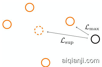
Figure 2: An example of the geometric center issue. Orange circles are positive to the black circle instance, while the dotted orange circle is their geometric center. The difference between $\mathcal{L}{\mathrm{sup}}$ and our $\mathcal{L}_{\mathrm{max}}$ is that we target the closest positive instead of their geometric center.
图 2: 几何中心问题示例。橙色圆圈与黑色圆圈实例呈正相关,而虚线橙色圆圈是它们的几何中心。$\mathcal{L}{\mathrm{sup}}$ 与我们的 $\mathcal{L}_{\mathrm{max}}$ 的区别在于,我们以最近的正样本为目标,而非它们的几何中心。
contrastive hashing.
对比哈希
We begin by upgrading the CKY, which parses sentences, returns spans with discrete labels, to support binary format labels (§3.1). Subsequently, we define a new similarity function by using span marginal probabilities obtained from this bit-level CKY (§3.2) to jointly learn label and structural information. Furthermore, we conduct a detailed analysis of several widely used contrastive learning losses, identifying the geometric center issue, and introduce a novel contrastive learning loss to remedy it (§3.3) through carefully selecting instances. By doing so, we show that it is feasible to introduce binary representation to output layers and have them output binary labels on trees. Moreover, since our model is based on contrastive learning, it also benefits from its remarkable representation learning capability, resulting in better performance than existing models. We conduct experiments on constituency parsing and nested named entity recognition. Experimental results (§4.2) demonstrate that our models achieve competitive performance with only around 12 and 8 bits, respectively.
我们首先对CKY算法进行升级,使其在解析句子并返回带有离散标签的片段时,能够支持二进制格式标签(见3.1节)。随后,我们利用从这种比特级CKY算法获得的片段边际概率,定义了一种新的相似度函数,以联合学习标签和结构信息(见3.2节)。此外,我们对几种广泛使用的对比学习损失函数进行了详细分析,发现了几何中心问题,并通过精心选择实例引入了一种新的对比学习损失函数来解决该问题(见3.3节)。通过这种方式,我们证明了在输出层引入二进制表示并让它们在树上输出二进制标签是可行的。此外,由于我们的模型基于对比学习,它还能从其卓越的表征学习能力中受益,从而获得优于现有模型的性能。我们在成分句法分析和嵌套命名实体识别任务上进行了实验。实验结果(见4.2节)表明,我们的模型分别仅需约12比特和8比特就能达到具有竞争力的性能。
2 Background
2 背景
2.1 Constituency Parsing
2.1 成分句法分析
For a given sentence $w_{1},\ldots,w_{n}$ , constituency parsing aims at detecting its hierarchical syntactic structures. Previous work (Stern et al., 2017; Gaddy et al., 2018; Kitaev and Klein, 2018; Kitaev et al., 2019; Zhang et al., 2020) decompose tree score $g(t)$ as the sum of its constituents scores,
对于给定句子 $w_{1},\ldots,w_{n}$,成分句法分析旨在检测其层次化的句法结构。先前工作 (Stern et al., 2017; Gaddy et al., 2018; Kitaev and Klein, 2018; Kitaev et al., 2019; Zhang et al., 2020) 将树评分 $g(t)$ 分解为其组成成分得分的总和。
$$
g(\pmb{t})=\sum_{\langle l_{i},r_{i},y_{i}\rangle\in\pmb{t}}g(l_{i},r_{i},y_{i})
$$
$$
g(\pmb{t})=\sum_{\langle l_{i},r_{i},y_{i}\rangle\in\pmb{t}}g(l_{i},r_{i},y_{i})
$$
where $l_{i}$ and $r_{i}$ indicate the left and right boundary of the $i$ -th span, and $y_{i}\in\mathcal{V}$ stands for the label. Constituent score $g(l_{i},r_{i},y_{i})$ reflects the joint score of selecting the specified span and assigning it the specified label. Previous work (Kitaev and Klein, 2018; Zhang et al., 2020) commonly compute this score using a linear or bilinear component. Under the framework of graphical probabilistic models, they can efficiently compute the conditional probability by applying the CKY algorithm.
其中 $l_{i}$ 和 $r_{i}$ 表示第 $i$ 个跨度的左右边界,$y_{i}\in\mathcal{V}$ 代表标签。成分得分 $g(l_{i},r_{i},y_{i})$ 反映了选择指定跨度并为其分配指定标签的联合得分。先前的工作 (Kitaev and Klein, 2018; Zhang et al., 2020) 通常使用线性或双线性组件计算该得分。在图概率模型的框架下,它们可以通过应用CKY算法高效计算条件概率。
$$
p(\pmb{t})=\frac{\exp g(\pmb{t})}{Z\equiv\sum_{\pmb{t}^{\prime}\in\mathcal{T}}\exp g(\pmb{t}^{\prime})}
$$
$$
p(\pmb{t})=\frac{\exp g(\pmb{t})}{Z\equiv\sum_{\pmb{t}^{\prime}\in\mathcal{T}}\exp g(\pmb{t}^{\prime})}
$$
$Z$ is commonly known as the partition function which enumerates all valid constituency trees.
$Z$ 通常被称为配分函数 (partition function),用于枚举所有有效的成分树。
Besides, marginal probability $\mu(l_{i},r_{i},y_{i})$ is also frequently mentioned. It stands for the proportion of scores for all trees that include the specified span with the specified label. As noted by Eisner (2016), computing the partial derivative of the log partition with respect to the span score is an efficient approach to obtain the marginal probability.
此外,边缘概率 $\mu(l_{i},r_{i},y_{i})$ 也经常被提及。它表示包含指定跨度和指定标签的所有树的分数比例。正如 Eisner (2016) 所指出的,计算对数配分函数相对于跨度得分的偏导数是获得边缘概率的有效方法。
$$
\mu(l_{i},r_{i},y_{i})=\frac{\partial\log Z}{\partial g(l_{i},r_{i},y_{i})}
$$
$$
\mu(l_{i},r_{i},y_{i})=\frac{\partial\log Z}{\partial g(l_{i},r_{i},y_{i})}
$$
Intuitively, marginal probability indicates the joint probability of selecting a specified span with a specified label. Therefore, it is easy to notice that merely summing the marginal probabilities for all labels of a given span does not always yield 1, i.e., $\textstyle\sum_{y^{\prime}\in y}\mu(l_{i},r_{i},y^{\prime})\not\equiv1$ , as there is no guarantee t hat this span will be selected. In other words, marginal probabilities contain not only label information but also structural information. If a span is unlikely to be selected, its marginal probability will not be high regardless of the label.
直观上,边缘概率表示选择具有特定标签的特定跨度的联合概率。因此,很容易注意到,仅对给定跨度的所有标签的边缘概率求和并不总是等于1,即 $\textstyle\sum_{y^{\prime}\in y}\mu(l_{i},r_{i},y^{\prime})\not\equiv1$ ,因为无法保证该跨度会被选中。换句话说,边缘概率不仅包含标签信息,还包含结构信息。如果一个跨度不太可能被选中,那么无论标签如何,其边缘概率都不会很高。
2.2 Contrastive Hashing
2.2 对比哈希 (Contrastive Hashing)
Contrastive learning (He et al., 2020; Gao et al., 2021; Khosla et al., 2020) is an effective yet simple representation learning method, which involves pulling together positive pairs and pushing apart negative pairs in a metric space. Recently, Wang et al. (2023) extended this approach as contrastive hashing. They append an untrained transformer to the end of a pre-trained language model and use its attention scores for both task learning and hashing. Specifically, its entire attention probabilities $a_{i,j}^{k}$ are used to compute hidden states for downstream tasks as usual, and its diagonal entries sik,i of the attention scores are employed for hashing.
对比学习 (He et al., 2020; Gao et al., 2021; Khosla et al., 2020) 是一种简单高效的表征学习方法,其核心思想是在度量空间中拉近正样本对、推远负样本对。Wang等人 (2023) 近期将该方法扩展为对比哈希学习,他们在预训练语言模型末端接入未经训练的Transformer,并利用其注意力分数同时进行任务学习和哈希生成。具体而言,模型像常规下游任务一样使用全部注意力概率 $a_{i,j}^{k}$ 计算隐藏状态,同时采用注意力分数矩阵的对角元素 $s_{i}^{k,i}$ 进行哈希编码。
$$
\begin{array}{c}{{s_{i,j}^{k}=\frac{(\mathbf{W}{k}^{Q}{h_{i}})^{\top}(\mathbf{W}{k}^{K}{h_{j}})}{\sqrt{d_{k}}}}}\ {{a_{i,j}^{k}=\displaystyle\mathrm{softmax}\left(s_{i,j}^{k}\right)}}\end{array}
$$
$$
\begin{array}{c}{{s_{i,j}^{k}=\frac{(\mathbf{W}{k}^{Q}{h_{i}})^{\top}(\mathbf{W}{k}^{K}{h_{j}})}{\sqrt{d_{k}}}}}\ {{a_{i,j}^{k}=\displaystyle\mathrm{softmax}\left(s_{i,j}^{k}\right)}}\end{array}
$$
Where WQ and WkK are parameters, h are hidden states, $d_{k}$ is the head dimension. These two learning objectives share the same attention matrix, therefore, task-relevant information is implicitly ensured to be preserved in these binary codes.
其中 WQ 和 WkK 是参数,h 是隐藏状态,$d_{k}$ 是头维度。这两个学习目标共享相同的注意力矩阵,因此任务相关信息被隐式地确保保留在这些二进制代码中。
More specifically, to leverage the multi-head mechanism, they allow each head to represent one and only one bit. By increasing the number of heads to $K$ , they obtain attention scores from $K$ different semantic aspects. During the inference stage, codes are generated by binarizing these scores,
具体来说,为利用多头机制,他们让每个头仅表示一个比特。通过将头数增至$K$,他们从$K$个不同语义维度获得注意力分数。在推理阶段,通过二值化这些分数生成编码。
$$
\begin{array}{c}{{\pmb{c}{i}=[c_{i}^{1},\cdots,c_{i}^{K}]\in{-1,+1}^{K}}}\ {{\pmb{c}{i}^{k}=\mathrm{sign}(s_{i,i}^{k})}}\end{array}
$$
$$
\begin{array}{c}{{\pmb{c}{i}=[c_{i}^{1},\cdots,c_{i}^{K}]\in{-1,+1}^{K}}}\ {{\pmb{c}{i}^{k}=\mathrm{sign}(s_{i,i}^{k})}}\end{array}
$$
During the training stage, they approximate Hamming similarity by computing the cosine similarity, with one of its inputs binarized first.
在训练阶段,他们通过计算余弦相似度来近似汉明相似度 (Hamming similarity) ,其中一个输入会先进行二值化处理。
$$
s(i,j)=\cos\left({s_{i,i},c_{j}}\right)
$$
$$
s(i,j)=\cos\left({s_{i,i},c_{j}}\right)
$$
Apart from this similarity function, they also propose a novel loss by carefully selecting instances and eliminating potential positives and negatives. They fine-tune the entire model using both the downstream task loss and the contrastive hashing loss, i.e., $\mathcal{L}=\mathcal{L}{\mathrm{task}}+\beta\cdot\mathcal{L}_{\mathrm{contrastive}}$ . Experiments show that they can reproduce the original performance on an extremely tiny model using only these 24-bit codes as inputs. Therefore, they claim that these codes preserve all the necessary task-relevant information.
除了这种相似性函数外,他们还通过精心选择实例并消除潜在的正面和负面样本,提出了一种新颖的损失函数。他们结合下游任务损失和对比哈希损失对完整模型进行微调,即 $\mathcal{L}=\mathcal{L}{\mathrm{task}}+\beta\cdot\mathcal{L}_{\mathrm{contrastive}}$ 。实验表明,仅使用这些24位编码作为输入,就能在极小型模型上复现原始性能。因此,他们宣称这些编码保留了所有必要的任务相关信息。
3 Proposed Methods
3 研究方法
Our model attempts to learn parsing and hashing simultaneously with a single structured contrastive hashing loss. In other words, we try to introduce the binary representation to output layers and eliminate the need for the $\mathcal{L}_{\mathrm{task}}$ above. To achieve this, we first extend the CKY module to support binary labels (§3.1). Then, we replace the cosine similarity with a newly defined similarity function (§3.2) based on span marginal probabilities, because it contains not only label information but also structural information. After that, we analyze several commonly used contrastive losses, and propose a new one (§3.3) to mitigate the geometric center issue as shown in Figure 2. After training, we build code vocabulary by mapping binary codes back to their most frequently coinciding labels.
我们的模型尝试通过单一的结构化对比哈希损失函数同时学习解析和哈希。换句话说,我们试图将二进制表示引入输出层,从而消除上述 $\mathcal{L}_{\mathrm{task}}$ 的需求。为此,我们首先扩展CKY模块以支持二进制标签(见第3.1节)。接着,我们用一个基于跨度边缘概率的新定义相似度函数(见第3.2节)替代余弦相似度,因为它不仅包含标签信息,还包含结构信息。之后,我们分析了几种常用的对比损失函数,并提出了一种新的损失函数(见第3.3节)以缓解如图2所示的几何中心问题。训练完成后,我们通过将二进制代码映射回其最常对应的标签来构建代码词汇表。
3.1 Constituency Parsing with Bits
3.1 基于比特的选区解析
We decompose tree scores as the sum of constituent scores as well, but with discrete labels $y_{i}$ replaced with binary codes $\pmb{c}_{i}\in{-1,+1}^{K}$ .
我们将树得分同样分解为组成得分的总和,但将离散标签 $y_{i}$ 替换为二进制编码 $\pmb{c}_{i}\in{-1,+1}^{K}$。
$$
g(\pmb{t})=\sum_{\langle l_{i},r_{i},\pmb{c}{i}\rangle\in\pmb{t}}g(l_{i},r_{i},\pmb{c}_{i})
$$
$$
g(\pmb{t})=\sum_{\langle l_{i},r_{i},\pmb{c}{i}\rangle\in\pmb{t}}g(l_{i},r_{i},\pmb{c}_{i})
$$
$$
g(l_{i},r_{i},c_{i})=\sum_{k=1}^{K}g_{k}(l_{i},r_{i},c_{i}^{k})
$$
$$
g(l_{i},r_{i},c_{i})=\sum_{k=1}^{K}g_{k}(l_{i},r_{i},c_{i}^{k})
$$
Where $g_{k}(l_{i},r_{i},c_{i}^{k})$ represents the span score with the $k$ -th bit position assigned as value $c_{i}^{k}$ . We additionally assume that the bits are independent of each other, so we simply add their scores together to obtain the span score $g(l_{i},r_{i},\pmb{c}_{i})$ .
其中 $g_{k}(l_{i},r_{i},c_{i}^{k})$ 表示第 $k$ 个比特位赋值为 $c_{i}^{k}$ 时的跨度得分。我们进一步假设各比特位相互独立,因此只需将它们的得分相加即可得到跨度得分 $g(l_{i},r_{i},\pmb{c}_{i})$。
Following Wang et al. (2023), we maintain the one-head-one-bit design and also utilize attention scores for hashing. Furthermore, since we attempt to eliminate $\mathcal{L}{\mathrm{task}}$ , we do not need to compute the final outputs of the transformer layer. Therefore, we only retain the query $\mathbf{W}{k}^{Q}$ and key $\mathbf{W}{k}^{K}$ to calculate the span score for getting $+1$ in the $k$ -th bit position by using the token hidden states of the left and right span boundary $\pmb{h}{l_{i}}$ and $h_{r_{i}}$ . For the $-1$ case, we simply leave its score as 0.
遵循Wang等人 (2023) 的研究,我们保持一头一比特的设计,并继续使用注意力分数进行哈希处理。此外,由于我们尝试消除 $\mathcal{L}{\mathrm{task}}$ ,因此无需计算transformer层的最终输出。因此,我们仅保留查询矩阵 $\mathbf{W}{k}^{Q}$ 和键矩阵 $\mathbf{W}{k}^{K}$ ,通过左右边界token的隐藏状态 $\pmb{h}{l_{i}}$ 和 $h_{r_{i}}$ 来计算跨度得分,从而在第 $k$ 比特位获得 $+1$ 。对于 $-1$ 的情况,我们直接将其得分设为0。
$$
\begin{array}{r l}&{g_{k}(l_{i},r_{i},+1)=\frac{(\mathbf{W}{k}^{Q}{h_{l_{i}}})^{\top}(\mathbf{W}{k}^{K}{h_{r_{i}}})}{\sqrt{d_{k}}}}\ &{g_{k}(l_{i},r_{i},-1)=0}\end{array}
$$
$$
\begin{array}{r l}&{g_{k}(l_{i},r_{i},+1)=\frac{(\mathbf{W}{k}^{Q}{h_{l_{i}}})^{\top}(\mathbf{W}{k}^{K}{h_{r_{i}}})}{\sqrt{d_{k}}}}\ &{g_{k}(l_{i},r_{i},-1)=0}\end{array}
$$
With these definitions, we can extend the CKY module to the bit-level and calculate the conditional probability and partition function using Equation 2 as usual. Additionally, the bit-level marginal probability is defined as below.
根据这些定义,我们可以将CKY模块扩展到比特级别,并像往常一样使用公式2计算条件概率和配分函数。此外,比特级边际概率定义如下。
$$
\mu_{k}(l_{i},r_{i},c_{i}^{k})=\frac{\partial\log Z}{\partial g_{k}(l_{i},r_{i},c_{i}^{k})}
$$
$$
\mu_{k}(l_{i},r_{i},c_{i}^{k})=\frac{\partial\log Z}{\partial g_{k}(l_{i},r_{i},c_{i}^{k})}
$$
3.2 Contrastive Hashing with Structures
3.2 结构化对比哈希
Wang et al. (2023) emphasize that the key to their loss function is first hashing one of its inputs as codes and then calculating the similarity between continuous scores and the discrete codes. We define our similarity function in a similar way. Since we can straightforwardly obtain the span marginal probabilities with Equation 12, we then binarize scores into codes towards the sides with the higher span marginal probabilities.
Wang等 (2023) 强调其损失函数的关键在于先将其中一个输入哈希为离散编码 (codes) ,再计算连续分数与离散编码之间的相似度。我们以类似方式定义相似度函数。由于可通过公式12直接获得片段边际概率 (span marginal probabilities) ,我们随后将分数二值化为偏向更高片段边际概率侧的编码。
$$
\pmb{c}{i}=[c_{i}^{1},\dots,c_{i}^{K}]\in{-1,+1}^{K}
$$
$$
\pmb{c}{i}=[c_{i}^{1},\dots,c_{i}^{K}]\in{-1,+1}^{K}
$$
Naturally, we define the similarity function between two spans as the marginal probability of selecting $i$ -th span while assigning $c_{j}$ as its code.
我们自然地将两个片段之间的相似度函数定义为在将$c_{j}$分配为其代码时选择第$i$个片段的边际概率。
$$
s(i,j)=\frac{1}{K}\sum_{k=1}^{K}\mu_{k}(l_{i},r_{i},c_{j}^{k})
$$
$$
s(i,j)=\frac{1}{K}\sum_{k=1}^{K}\mu_{k}(l_{i},r_{i},c_{j}^{k})
$$
As we mentioned above (§2.1), we use marginal probabilities to define the similarity function because they reflect the joint probability of both selecting the specified span and assigning the specified label to it. If a span is unlikely to be selected as a phrase, then both $\mu_{k}(l_{i},r_{i},+1)$ and $\mu_{k}(l_{i},r_{i},-1)$ will be close to zero. Thus, the model learns structural and label information simultaneously. By leveraging this similarity function, we extend contrastive hashing to structured contrastive hashing. This approach eliminates the label embedding from the output layer, as the hashing layer returns labels in binary format now.
正如上文所述(§2.1),我们使用边缘概率来定义相似度函数,因为它们反映了同时选中指定文本片段并为其分配指定标签的联合概率。若某文本片段不太可能被选为短语,则$\mu_{k}(l_{i},r_{i},+1)$和$\mu_{k}(l_{i},r_{i},-1)$都将趋近于零。因此,该模型能同步学习结构信息和标签信息。通过运用该相似度函数,我们将对比哈希扩展为结构化对比哈希。这种方法从输出层移除了标签嵌入,因为哈希层现在以二进制格式返回标签。
Moreover, for a sentence with $n$ tokens, the total number of spans is $(n^{2}+n)/2$ , and bit-level CKY returns marginal probabilities for them all. However, using them for contrastive hashing leads to an intractable time complexity of $\mathcal{O}(n^{4})$ . In practice, we select only spans from the target trees, reducing the number of spans to $2n-1$ to maintain the time complexity at ${\mathcal{O}}(n^{2})$ . This is another reason why we prefer marginal probability.
此外,对于一个包含 $n$ 个 token 的句子,其总跨度数为 $(n^{2}+n)/2$,而比特级 CKY 会返回所有这些跨度的边缘概率。但若将其用于对比哈希,将导致 $\mathcal{O}(n^{4})$ 的难以处理的时间复杂度。实践中,我们仅从目标树中选择跨度,将跨度数降至 $2n-1$,从而将时间复杂度维持在 ${\mathcal{O}}(n^{2})$。这也是我们更倾向于使用边缘概率的另一个原因。
3.3 Instance Selection
3.3 实例选择
Following the contrastive learning framework (Gao et al., 2021; Wang et al., 2023), we feed sentences into the neural network twice to obtain two semantically identical but slightly augmented represent at ions. In this way, we get two different marginal probabilities for each span. We calculate contrastive losses by comparing each span across views and average them as the batch loss (§3.5). Note that each batch contains spans from multiple sentences, so our contrastive hashing also compares spans across different sentences. For clarity, we omit subscripts in the following equations when there is no ambiguity.
遵循对比学习框架 [Gao et al., 2021; Wang et al., 2023],我们将句子两次输入神经网络,获得两个语义相同但经过轻微增强的表示。通过这种方式,每个片段会得到两个不同的边缘概率。我们通过跨视图比较每个片段来计算对比损失,并将其平均值作为批次损失(§3.5)。需要注意的是,每个批次包含来自多个句子的片段,因此我们的对比哈希还会比较不同句子间的片段。为简洁起见,下文公式在不引起歧义的情况下省略下标。
As we mentioned above (§2.2), the fundamental concept of contrastive learning is pulling together positives and pushing apart negatives. The most commonly used objective function is defined as,
正如上文所述(§2.2),对比学习(contrastive learning)的核心思想是拉近正样本、推远负样本。最常用的目标函数定义为:
$$
\mathcal{L}{\mathrm{self}}=-\log\frac{\exp s(i,i)}{\sum_{j\in\mathcal{N}\cup\mathcal{P}}\exp s(i,j)}
$$
$$
\mathcal{L}{\mathrm{self}}=-\log\frac{\exp s(i,i)}{\sum_{j\in\mathcal{N}\cup\mathcal{P}}\exp s(i,j)}
$$
$\mathcal{N}={j\mid y_{j}\neq y_{i}}$ and $\mathcal{P}={j\mid y_{j}=y_{i}}$ stands for the negative and positive sets, respectively. We additionally define ${\cal{S}}={i}$ as the set that contains span $i$ as its only entry. It is obvious that ${\mathcal{S}}\subseteq{\mathcal{P}}$ always holds.
$\mathcal{N}={j\mid y_{j}\neq y_{i}}$ 和 $\mathcal{P}={j\mid y_{j}=y_{i}}$ 分别代表负样本集和正样本集。我们额外定义 ${\cal{S}}={i}$ 为仅包含跨度 $i$ 的集合。显然 ${\mathcal{S}}\subseteq{\mathcal{P}}$ 恒成立。
In addition, the $\log\sum$ exp operator is commonly considered a differen tiable approximation of the max operator. Therefore, by slightly tweaking the equation, we reinterpret it as below.
此外,$\log\sum$ exp 算子通常被视为 max 算子的可微近似。因此,通过略微调整方程,我们将其重新解释如下。
$$
\begin{array}{r l}{\lefteqn{\mathcal{L}{\mathrm{self}}=\log\sum_{j}\exp s(i,j)-s(i,i)}}\ &{\approx\underset{j\in\mathcal{N}\cup\mathcal{P}}{\operatorname*{max}}s(i,j)-s(i,i)}\end{array}
$$
$$
\begin{array}{r l}{\lefteqn{\mathcal{L}{\mathrm{self}}=\log\sum_{j}\exp s(i,j)-s(i,i)}}\ &{\approx\underset{j\in\mathcal{N}\cup\mathcal{P}}{\operatorname*{max}}s(i,j)-s(i,i)}\end{array}
$$
Moreover, Khosla et al. (2020) also proposed a loss function for supervised settings where multiple positives are present. By applying the same tricks, we can rewrite the loss function as follows.
此外,Khosla等人 (2020) 还针对存在多个正样本的监督场景提出了一种损失函数。通过应用相同的技巧,我们可以将该损失函数改写如下。
$$
\begin{array}{r}{\mathcal{L}{\operatorname*{sup}}=-\displaystyle\frac{1}{|\mathcal{P}|}\sum_{p\in\mathcal{P}}\log\displaystyle\frac{\exp s(i,p)}{\sum_{j\in\mathcal{N}\cup\mathcal{P}}\exp s(i,j)}}\ {=\log\displaystyle\sum_{j}\exp s(i,j)-\displaystyle\frac{1}{|\mathcal{P}|}\sum_{p}s(i,p)}\ {\approx\displaystyle\operatorname*{max}_{j\in\mathcal{N}\cup\mathcal{P}}s(i,j)-\displaystyle\operatorname*{mean}_{j\in\mathcal{P}}s(i,j)\qquad(}\end{array}
$$
$$
\begin{array}{r}{\mathcal{L}{\operatorname*{sup}}=-\displaystyle\frac{1}{|\mathcal{P}|}\sum_{p\in\mathcal{P}}\log\displaystyle\frac{\exp s(i,p)}{\sum_{j\in\mathcal{N}\cup\mathcal{P}}\exp s(i,j)}}\ {=\log\displaystyle\sum_{j}\exp s(i,j)-\displaystyle\frac{1}{|\mathcal{P}|}\sum_{p}s(i,p)}\ {\approx\displaystyle\operatorname*{max}_{j\in\mathcal{N}\cup\mathcal{P}}s(i,j)-\displaystyle\operatorname*{mean}_{j\in\mathcal{P}}s(i,j)\qquad(}\end{array}
$$
Wang et al. (2023) have also proposed a contrastive loss function for hashing. They claim that identical tokens may even not contain identical information due to different contexts. Therefore, they treat $\mathcal{P}$ as potential false positives and negatives, and replace it with $s$ in both terms.
Wang等人 (2023) 还提出了一种用于哈希的对比损失函数。他们认为由于上下文不同,相同的token甚至可能不包含相同的信息。因此,他们将$\mathcal{P}$视为潜在的假阳性和假阴性,并在两项中用$s$替换它。
$$
\begin{array}{r l r}{\lefteqn{\mathcal{L}{\mathrm{hash}}=-\log\frac{\exp s(i,i)}{\sum_{j\in\mathcal{N}\cup\cal{S}}\exp s(i,j)}}}\ &{}&{\approx\underset{j\in\mathcal{N}\cup\cal{S}}{\operatorname*{max}}s(i,j)-s(i,i)\quad\quad}\end{array}
$$
$$
\begin{array}{r l r}{\lefteqn{\mathcal{L}{\mathrm{hash}}=-\log\frac{\exp s(i,i)}{\sum_{j\in\mathcal{N}\cup\cal{S}}\exp s(i,j)}}}\ &{}&{\approx\underset{j\in\mathcal{N}\cup\cal{S}}{\operatorname*{max}}s(i,j)-s(i,i)\quad\quad}\end{array}
$$
By unifying them all in a common format, we can observe that their main differences lie in the instance selection strategies. Both $\mathcal{L}{\mathrm{self}}$ and $\mathcal{L}{\mathrm{sup}}$ pull instances towards the geometric center of their positive instances in the second term . The only difference is that $\mathcal{L}{\mathrm{self}}$ assumes there is only one positive instance, making the geometric center merely $i$ -th span itself, whereas $\mathcal{L}{\mathrm{sup}}$ has access to the groundtruth labels and thus can obtain a more specific center. On the other hand, $\mathcal{L}{\mathrm{hash}}$ differs from $\mathcal{L}{\mathrm{self}}$ in the first term , as it suggests that dividing instances solely based on ground-truth labels may also introduce false positives and negatives. Therefore, ${\mathcal{L}}_{\mathrm{hash}}$ excludes potential false positives from this term. Additionally, it is noteworthy that among these three losses, all first terms employ max, while all second terms use mean. Intuitively speaking, the max operator pulls towards the most likely true positive instance, while mean operator pulls towards the geometric center of all positive instances. Although it is hard to determine whether instances in $\mathcal{P}$ are false positives or not, what we can be certain of is that there is at least one true positive instance, since $S\subseteq{\mathcal{P}}$ always holds. Therefore, using the max operator to pull towards the most probable one is a more effective approach.
通过将它们统一为通用格式,我们可以观察到其主要差异在于实例选择策略。$\mathcal{L}{\mathrm{self}}$ 和 $\mathcal{L}{\mathrm{sup}}$ 的第二项都将实例拉向正例的几何中心,唯一区别在于 $\mathcal{L}{\mathrm{self}}$ 假设仅存在单个正例(几何中心即第 $i$ 个跨度自身),而 $\mathcal{L}{\mathrm{sup}}$ 能利用真实标签获得更精确的中心。相比之下,$\mathcal{L}{\mathrm{hash}}$ 在第一项与 $\mathcal{L}{\mathrm{self}}$ 存在差异——该损失认为仅基于真实标签划分实例仍可能引入假正例和假反例,因此 ${\mathcal{L}}_{\mathrm{hash}}$ 排除了该部分潜在的假正例。值得注意的是,这三个损失函数的第一项均采用 max 运算,第二项则使用 mean 运算。直观而言,max 运算将实例拉向最可能的真正例,而 mean 运算拉向所有正例的几何中心。尽管难以判定 $\mathcal{P}$ 中的实例是否为假正例,但可以确定至少存在一个真正例(因 $S\subseteq{\mathcal{P}}$ 恒成立),因此采用 max 运算拉向最可能实例是更有效的策略。
$$
\begin{array}{r l}&{\mathcal{L}{\mathrm{max}}\approx\underset{j\in\mathcal{N}\cup\mathcal{S}}{\mathrm{max}}s(i,j)-\underset{j\in\mathcal{P}}{\mathrm{max}}s(i,j)}\ &{\quad\quad\approx\underset{j\in\mathcal{N}\cup\mathcal{S}}{\mathrm{log}}\underset{j\in\mathcal{N}\cup\mathcal{S}}{\sum}\exp s(i,j)}\ &{\qquad-\underset{p\in\mathcal{P}}{\mathrm{log}}\exp s(i,p)}\ &{\quad\quad=-\log\frac{\sum_{p\in\mathcal{P}}\exp s(i,p)}{\sum_{j\in\mathcal{N}\cup\mathcal{S}}\exp s(i,j)}}\end{array}
$$
3.4 Architecture
3.4 架构
As shown in Figure 1, our model consists of a pretrained language model, an attention hash layer, and a bit-level CKY. The attention hash layer derives from the transformer layer, but it preserves only the query and key components for calculating span score $g(l_{i},r_{i},\pmb{c}_{i})$ . All the other components, such as layer normalization (Ba et al., 2016) and feed-forward layers, are removed, as there is no need to calculate hidden states.
如图 1 所示,我们的模型由预训练语言模型、注意力哈希层和位级 CKY 组成。注意力哈希层源自 transformer 层,但仅保留查询(query)和键(key)组件用于计算跨度得分 $g(l_{i},r_{i},\pmb{c}_{i})$ 。其他所有组件,例如层归一化 (Ba et al., 2016) 和前馈层都被移除,因为无需计算隐藏状态。
Compared with existing constituency parsers (Kitaev and Klein, 2018; Zhang et al., 2020), the output layer of our parser does not include label embedding matrices. Instead, it utilizes the attention hash layer and a bit-level CKY to predict the binary representation of labels. Consequently, the number of parameters of this part changes from $|\mathcal{D}|\times d$ to two $K\times\lceil\frac{d}{K}\rceil\times d$ .
与现有成分句法分析器 (Kitaev and Klein, 2018; Zhang et al., 2020) 相比,我们的分析器输出层不包含标签嵌入矩阵,而是利用注意力哈希层和位级CKY来预测标签的二进制表示。因此,这部分参数数量从 $|\mathcal{D}|\times d$ 变为两个 $K\times\lceil\frac{d}{K}\rceil\times d$。
3.5 Training and Inference
3.5 训练与推理
During the training stage, we feed sentences into the model twice to obtain marginal probabilities $\mu^{1}$ and $\mu^{2}$ of the two views, and binarize spans on the target trees $\hat{t}^{1}={\langle l_{i},r_{i},\pmb{c}{i}^{1}\rangle}{i=1}^{2n-1}$ and $\hat{t}^{2}= {\langle l_{i},r_{i},c_{i}^{2}\rangle}{i=1}^{2n-1}$ using Equatio n 13, respectively. Besides, we use the ground-truth labels $y_{i}$ to divide $\mathcal{N}$ and $\mathcal{P}$ . After that, we calculate the contrastive hashing loss for each span with Equation 19 and average them as the batch loss.
在训练阶段,我们将句子两次输入模型以获得两个视图的边际概率$\mu^{1}$和$\mu^{2}$,并分别使用公式13对目标树$\hat{t}^{1}={\langle l_{i},r_{i},\pmb{c}{i}^{1}\rangle}{i=1}^{2n-1}$和$\hat{t}^{2}= {\langle l_{i},r_{i},c_{i}^{2}\rangle}{i=1}^{2n-1}$上的跨度进行二值化。此外,我们使用真实标签$y_{i}$来划分$\mathcal{N}$和$\mathcal{P}$。之后,我们使用公式19计算每个跨度的对比哈希损失,并将其平均作为批次损失。
$$
\mathcal{L}=\operatorname*{mean}_{1\leq i<2n}\left(\mathcal{L}(i,\mu^{1},\hat{\pmb{t}}^{2})+\mathcal{L}(i,\mu^{2},\hat{\pmb{t}}^{1})\right)
$$
$$
\mathcal{L}=\operatorname*{mean}_{1\leq i<2n}\left(\mathcal{L}(i,\mu^{1},\hat{\pmb{t}}^{2})+\mathcal{L}(i,\mu^{2},\hat{\pmb{t}}^{1})\right)
$$
Table 1: The constituency parsing results. The bold numbers and the underlined numbers indicate the best and the second-best performance of each column. $b\sharp\diamond$ stands for the graph-based, transition-based, and sequence-to-sequence models, respectively.
表 1: 选区解析结果。加粗数字和下划线数字分别表示每列最优和次优性能。$b\sharp\diamond$ 分别代表基于图、基于转移和序列到序列模型。
| MODEL | PTB | CTB BERT |
|---|---|---|
| BERT | XLNET | |
| Kitaev et al. (2019)b | 95.59 | |
| Zhou and Zhao (2019)* | 95.84 | 96.33 |
| Mrini et al. (2020) | 96.38 | |
| Zhang et al. (2020)b | 95.69 | |
| Yang and Deng (2020)# | 95.79 | 96.34 |
| Tian et al. (2020) | 95.86 | 96.40 |
| Nguyen et al. (2021) | 95.70 | |
| Xin et al. (2021)b | 95.92 | |
| Cui et al. (2022)b | 95.92 | |
| Yang and Tu (2022) | 96.01 | |
| Yang and Tu (2023) Ours (6 bits)b | 96.04 | 96.48 |
| 94.81 | 95.70 | |
| Ours (8 bits)b | 95.95 | 96.34 |
| Ours (10 bits)b | 96.03 | 96.37 |
| Ours (12 bits) | 96.00 | 96.36 |
| Ours (14 bits) | ||
| 96.02 | 96.43 | |
| Ours (16 bits) | 95.98 | 96.40 |
After training, we switch the model to evaluation mode, i.e., turning off dropouts (Srivastava et al., 2014), and then feed all the training sentences into the model again. During this pass, we count the frequency of each pair of binary code and its corresponding ground-truth label, i.e., $f(c,y)$ . Then, we can reconstruct a code vocabulary to map codes back to their most frequently coinciding labels.
训练完成后,我们将模型切换到评估模式 (即关闭 dropout (Srivastava et al., 2014)),然后再次将所有训练句子输入模型。在此过程中,我们统计每对二进制代码及其对应真实标签的出现频率,即 $f(c,y)$。随后,可以重建一个代码词汇表,将代码映射回其最常对应的标签。
$$
\mathcal{Y}{\pmb{c}}\gets\arg\operatorname*{max}_{\boldsymbol{y}\in\mathcal{Y}}f(\pmb{c},\boldsymbol{y})
$$
$$
\mathcal{Y}{\pmb{c}}\gets\arg\operatorname*{max}_{\boldsymbol{y}\in\mathcal{Y}}f(\pmb{c},\boldsymbol{y})
$$
During the inference stage, we search the most probable tree from all valid trees using the CockeKasami-Younger (CKY) algorithm (Kasami, 1966). Our bit-level parsers return span boundaries and their binary codes, we translate them back to labels by using the Equation above.
在推理阶段,我们使用Cocke-Kasami-Younger (CKY)算法 (Kasami, 1966) 从所有有效树中搜索概率最高的树。我们的比特级解析器返回跨度边界及其二进制代码,通过上述方程将其转换回标签。
4 Experiments
4 实验
4.1 Settings
4.1 设置
We validate the effectiveness of our model on various structured prediction tasks, i.e., constituency parsing and nested named entity recognition tasks. Dataset statistics can be found in Appendix A.
我们在多种结构化预测任务上验证了模型的有效性,包括成分句法分析和嵌套命名实体识别任务。数据集统计信息详见附录A。
For the constituency parsing task, we conduct experiments on the datasets PTB (Marcus et al.,
在成分句法分析任务中,我们在PTB数据集 (Marcus et al., [20]) 上进行了实验。
Table 2: The nested named entity recognition results. $\tt b=\tt{7}\textbar{<}\textbar{>}$ stands for graph-based, span-based, sequential labeling, and sequence-to-sequence models, respectively.
表 2: 嵌套命名实体识别结果。$\tt b=\tt{7}\textbar{<}\textbar{>}$ 分别代表基于图、基于片段、序列标注和序列到序列模型。
| MODEL | ACE'4 BERT | ACE'5 BERT | GENIA BERT |
|---|---|---|---|
| Wang et al. (2020) | 86.28 | 84.66 | 79.19 |
| Wang et al. (2021) | 86.06 | 84.71 | 78.67 |
| Xu et al. (2021) | 86.30 | 85.40 | 79.60 |
| Fu et al. (2021)b | 86.60 | 85.40 | 78.20 |
| Yu et al. (2020) | 86.70 | 85.40 | 80.50 |
| Shen et al. (2021) | 87.41 | 86.67 | 80.54 |
| Tan et al. (2021) | 87.26 | 87.05 | 80.44 |
| Lou et al. (2022) | 87.90 | 86.91 | 78.44 |
| Zhu and Li (2022) | 87.98 | 87.15 | |
| Yang and Tu (2022) | 86.94 | 85.53 | 78.16 |
| Ours (4 bits)b | 85.81 | 83.37 | 73.54 |
| Ours (6 bits)b | 87.39 | 85.23 | 78.57 |
| Ours (8 bits)b | 87.93 | 85.90 | 78.79 |
| Ours (10 bits)b | 87.87 | 85.75 | 78.72 |
| Ours (12 bits)b | 87.52 | 85.26 | 78.40 |
- and CTB5.1 (Xue et al., 2005). We trans- form the original trees into those of Chomsky normal form and adopt left b inari z ation with NLTK (Bird and Loper, 2004). We study model performance by employing pre-trained language models with checkpoints bert-large-cased (Devlin et al., 2019) and xlnet-large-cased (Yang et al., 2019) for PTB, and bert-base-chinese for CTB.
- 和 CTB5.1 (Xue et al., 2005)。我们将原始树转换为乔姆斯基范式 (Chomsky normal form) ,并使用 NLTK (Bird and Loper, 2004) 进行左二元化。通过采用预训练语言模型评估模型性能:对 PTB 使用 bert-large-cased (Devlin et al., 2019) 和 xlnet-large-cased (Yang et al., 2019) 检查点,对 CTB 使用 bert-base-chinese。
For nested named entity recognition task, we use datasets ACE2004 (Doddington et al., 2004), ACE2005 (Walker et al., 2006), and GENIA (Kim et al., 2003). We follow the data splitting of Shibuya and Hovy (2020). Nested named entity recognition, as Fu et al. (2021) claimed, can be considered as a partially observed constituency parsing task. Therefore, we add a dummy span TOP as the top span to each sentence to ensure all the observed spans form a valid parsing tree, and apply the same transformation and b inari z ation on it. We use the checkpoint bert-large-cased on ACE2004 and ACE2005, and for the GENIA dataset we use dmis-lab/biobert-large-cased-v1.1 (Lee et al., 2019) as the pre-trained language model.
对于嵌套命名实体识别任务,我们使用数据集ACE2004 (Doddington et al., 2004)、ACE2005 (Walker et al., 2006)和GENIA (Kim et al., 2003)。我们遵循Shibuya和Hovy (2020)的数据划分方式。如Fu等人 (2021)所述,嵌套命名实体识别可视为部分观测的选区解析任务。因此,我们在每个句子中添加虚拟跨度TOP作为顶层跨度,以确保所有观测到的跨度形成有效的解析树,并对其应用相同的转换和二元化处理。在ACE2004和ACE2005数据集上使用bert-large-cased检查点,对于GENIA数据集则采用dmis-lab/biobert-large-cased-v1.1 (Lee et al., 2019)作为预训练语言模型。
We utilize the deep learning framework PyTorch (Paszke et al., 2019) to implement our models and download pre-trained lanugage checkpoints from hugging face/transformers (Wolf et al., 2020).
我们使用深度学习框架 PyTorch (Paszke et al., 2019) 实现模型,并从 hugging face/transformers (Wolf et al., 2020) 下载预训练语言检查点。
To keep the training of contrastive hashing stable, we collect sentences until the total number of tokens in each batch reaches 1024. We employ Adam optimizer (Kingma and Ba, 2015; Loshchilov and Hutter, 2019), and the total number of training steps of constituency parsing and nested named entity recognition are 50,000 and 20,000, and the warm-up are 4000 and 2000 steps, respectively. To provide harder negatives by augmenting inputs, we also randomly mask a portion of tokens as [MASK].
为使对比哈希训练保持稳定,我们收集句子直至每批token总数达到1024。采用Adam优化器 (Kingma and Ba, 2015; Loshchilov and Hutter, 2019),其中成分句法分析和嵌套命名实体识别的训练步数分别为50,000和20,000,预热步数分别为4000和2000步。为通过输入增强提供更难负样本,我们还随机将部分token掩码为[MASK]。
Table 3: Ablation study of instance selection strategies in constituency parsing experiments. The columns NEG and POS display the selection strategies for negatives and positives, respectively. LOSS shows this combination corresponds to which loss definition.
表 3: 选区解析实验中实例选择策略的消融研究。NEG和POS列分别显示负样本和正样本的选择策略。LOSS列显示该组合对应的损失定义。
| NEG | POS | LOSS | PTB |
|---|---|---|---|
| maxNUp | S | Lself | 81.08 |
| meanp | Lsup | 95.58 | |
| maxp | 95.75 | ||
| maxNus | S | Lhash | 94.26 |
| meanp | 95.88 | ||
| maxp | 96.03 |
Experiments are all conducted on a single NVIDIA Tesla V100 graphics card, the total training wall time is around 3 hours and 1 hour, respectively. All experiments are run with two different random seeds and the reported numbers in the following tables are their averages.
所有实验均在单张NVIDIA Tesla V100显卡上完成,总训练时间分别约为3小时和1小时。每组实验采用两种不同的随机种子运行,下文表格中报告的数据均为两次实验的平均值。
4.2 Main Results
4.2 主要结果
Our model consistently achieves competitive performance on various structured prediction tasks and datasets, as presented in Table 1 and Table 2.
我们的模型在各种结构化预测任务和数据集上始终展现出具有竞争力的性能,如表 1 和表 2 所示。
For constituency parsing, our models reach the peak with around 12 bits. Continuously increasing the number of bits does not further improve performance, on the contrary, it leads to a slight decline. We attribute this to the disproportionately large hashing space, as the amount of information carried by each task and dataset is fixed. For example, assigning $K$ bits to a task with only $K$ labels leads to an extreme case. Models in this case tend to produce the most trivial bit-level one-hot represent ation, making them nothing different from traditional static embedding models. On the contrary, decreasing the number of bits to fewer than 8 bits is also harmful, due to the insufficient representation capability. Besides, our models outperform almost all previous graph-based methods that rely on maximizing the log-likelihoods of target trees (Kitaev et al., 2019; Mrini et al., 2020; Zhang et al., 2020; Xin et al., 2021; Cui et al., 2022). There- fore, we claim that leveraging contrastive learning is beneficial to representation learning.
在成分句法分析任务中,我们的模型在12比特左右达到性能峰值。持续增加比特数不会带来性能提升,反而会导致轻微下降。我们认为这是由于哈希空间与任务信息量不匹配所致——每个任务和数据集承载的信息量是固定的。例如,为仅有$K$个标签的任务分配$K$比特会导致极端情况:模型倾向于生成最简单的比特级独热编码表示,使其与传统静态嵌入模型无异。反之,将比特数降至8比特以下也会因表征能力不足而损害性能。此外,我们的模型性能优于绝大多数基于目标树对数似然最大化的图方法 (Kitaev et al., 2019; Mrini et al., 2020; Zhang et al., 2020; Xin et al., 2021; Cui et al., 2022)。因此我们认为,对比学习对表征学习具有促进作用。
Table 4: Example of the hashing results on the constituency parsing task. The LABEL column shows the labels and their corresponding incomplete labels, which are introduced during the Chomsky normal form transformation. The CODE and COVERAGE columns display binary codes and their frequency proportions among all possible codes under each label. For instance, label $\mathsf{S}^{\star}$ is supposed to be assigned to an incomplete span within a larger S span, and $59.69%$ of $\mathsf{S}^{\flat}$ labels are translated from the code 101100001000.
表 4: 成分句法分析任务的哈希结果示例。LABEL列显示标签及其对应的不完整标签,这些标签是在乔姆斯基范式转换过程中引入的。CODE和COVERAGE列分别展示二进制代码及其在每个标签下所有可能代码中的频率占比。例如,标签$\mathsf{S}^{\star}$应被分配给较大S跨度内的不完整跨度,而$59.69%$的$\mathsf{S}^{\flat}$标签是从代码101100001000转换而来。
| LABEL | CODE | COVERAGE (%) |
|---|---|---|
| S | 110110001000 | 56.48 |
| 110100001101 | 42.80 | |
| S' | 101100001000 | 59.69 |
| 110110101001 | 38.36 | |
| NP | 010101001101 | 99.38 |
| NP' | 010001010100 | 98.70 |
| VP | 100010100111 | 99.52 |
| VP' | 001010010111 | 98.23 |
| ADJP | 100100000111 | 66.22 |
| 000011010110 | 29.08 | |
| ADJP' | 000000010110 | 93.34 |
| ADVP | 101100010111 | 84.53 |
| 000101100111 | 11.87 | |
| ADVP' | 001100010110 | 52.03 |
| 000101110110 | 37.00 |
For nested named entity recognition, all datasets show the best performance at the 8-bit settings, and decreasing to fewer than 6 bits also results in insufficient representing capability. Similarly, our methods outperform the previous sequential labeling methods (Shibuya and Hovy, 2020; Wang et al., 2021; Xin et al., 2021) and graph-based methods (Fu et al., 2021; Lou et al., 2022). In addition, some other papers (Yu et al., 2020; Shen et al., 2021; Tan et al., 2021; Zhu and Li, 2022) propose to straightforwardly enumerate all spans and directly train the model to classify them. These methods currently show the best performance, our method can also achieve comparable results to them.
在嵌套命名实体识别任务中,所有数据集在8位量化设置下均表现出最佳性能,当量化位数降至6位以下时会出现表征能力不足的情况。我们的方法同样优于先前的序列标注方法 (Shibuya and Hovy, 2020; Wang et al., 2021; Xin et al., 2021) 和图结构方法 (Fu et al., 2021; Lou et al., 2022)。此外,另有一些研究 (Yu et al., 2020; Shen et al., 2021; Tan et al., 2021; Zhu and Li, 2022) 提出直接枚举所有文本片段并进行分类训练的方案,这些方法目前保持着最优性能,而我们的方法也能取得与之相当的结果。
4.3 Ablation Studies
4.3 消融实验
We enumerate all combinations of the contrastive learning objective functions in Table 3 to study the influence of instance selection strategies.
我们在表3中列举了对比学习目标函数的所有组合,以研究实例选择策略的影响。
We note that selecting $\textstyle{\mathcal{N}}\cup S$ is always superior to selecting $\mathcal{N}\cup\mathcal{P}$ in the negative term , but using $s$ is inferior to using $\mathcal{P}$ in the positive term . This leads to the conclusion that adding positive instances $\mathcal{P}$ to the negative term is harmful, but it turns out to be beneficial when added to the positive term. This seems contradictory to the conclusion of Wang et al. (2023). However, this discrepancy arises because the training mechanisms are different. Their model relies on downstream task loss to implicitly learn structural information, whereas our model is designed to learn it explicitly. Therefore, we claim for the setting that aims at straightforwardly hashing both the label and structural information using a single loss, our $\mathcal{L}_{\mathrm{max}}$ is the best choice.
我们注意到,在负项中选择 $\textstyle{\mathcal{N}}\cup S$ 总是优于选择 $\mathcal{N}\cup\mathcal{P}$,但在正项中使用 $s$ 却不如使用 $\mathcal{P}$。由此得出结论:将正例 $\mathcal{P}$ 加入负项是有害的,但加入正项却有益。这一结论似乎与Wang等人(2023)的研究相矛盾。这种差异源于训练机制的不同:他们的模型依赖下游任务损失隐式学习结构信息,而我们的模型则显式学习这些信息。因此我们认为,对于旨在通过单一损失函数同时哈希标签和结构信息的设定,我们的 $\mathcal{L}_{\mathrm{max}}$ 是最佳选择。

Figure 3: Examples of the hashing and constituency parsing results. The hexadecimal numbers in the brackets indicate the generated binary codes, and the span labels are translated from them.
图 3: 哈希和选区解析结果示例。括号中的十六进制数字表示生成的二进制代码,跨度标签由这些代码转换而来。
Besides, Ouchi et al. (2020, 2021) appear to be the most relevant publications to our research. They also attempt to directly apply contrastive learning methods to structured prediction tasks. However, they pull instances towards the geometric centers, and their results show that this does not lead to noteworthy improvements than conventional graphbased models. This conclusion is consistent with ours, i.e., $\mathrm{max}{\mathscr P}$ is better than ${\mathrm{mean}}_{\mathcal{P}} $ . We hypothesize that calculating the geometric center largely erases the contextual information of each instance. Pulling towards this center is not essentially different from pulling towards a static label embedding. Therefore, their approach loses the advantage of contrastive learning and trivially falls back to the conventional static embedding classification. On the contrary, our $\mathrm{max}\mathcal{P}$ primarily targets the closest instance instead, therefore, it can fully leverage the capability of contrastive learning and distribute instances more uniformly, and allows each label to associate with multiple codes.
此外,Ouchi等人 (2020, 2021) 的论文似乎是与我们研究最相关的出版物。他们也尝试将对比学习方法直接应用于结构化预测任务。然而,他们将实例拉向几何中心,结果显示这种方法相比传统基于图的模型并未带来显著提升。这一结论与我们的发现一致,即 $\mathrm{max}{\mathscr P}$ 优于 ${\mathrm{mean}}_{\mathcal{P}}$。我们推测计算几何中心会大幅抹除每个实例的上下文信息。向该中心靠拢与向静态标签嵌入靠拢并无本质区别。因此,他们的方法丧失了对比学习的优势,简单地退化为传统的静态嵌入分类。相反,我们的 $\mathrm{max}\mathcal{P}$ 主要针对最近邻实例,因而能充分发挥对比学习能力,使实例分布更均匀,并允许每个标签关联多个编码。
4.4 Case Studies
4.4 案例分析
We show some frequent labels and their associated codes in Table 4. We only display the codes that occupy the top $90%$ frequency of each label. It can be observed that some labels have two codes with roughly the same frequency, while others are predominantly represented by a single code. However, even in these cases, none reach $100%$ coverage. This result further demonstrates that the term $\mathrm{max}_{\mathscr P}$ imposes only a weak supervision signal and does not force all instances towards the geometric centers, thereby avoiding false positives and allowing a more uniform distribution of instances, rather than crowding at a few specific points.
我们在表4中展示了一些高频标签及其关联代码。仅显示占各标签前90%频率的代码。可以观察到,部分标签有两个频率相近的代码,而其他标签则主要由单一代码主导。但即便在这些情况下,也没有代码能达到100%覆盖率。这一结果进一步证明,术语$\mathrm{max}_{\mathscr P}$仅提供弱监督信号,不会将所有实例强制推向几何中心,从而避免误判并保持实例更均匀的分布,而非聚集在少数特定点上。
In Figure 3, we display some parsing examples, using the same sentences as Wang et al. (2023). Our parser takes discrete tokens as inputs and returns binary labels, while theirs, conversely, receives binary codes of tokens and parses them into trees with discrete labels. Our codes preserve not only static by also contextual information of each label, for instance, the two S labels above are translated from two different codes. Therefore, our methods can also be considered as implicitly clustering methods, since these two codes refer to two different sub-labels of label S. This phenomenon is unlikely to be observed in models suffering from the geometric center issue.
图 3: 我们展示了一些解析示例,使用的句子与 Wang et al. (2023) 相同。我们的解析器以离散 token 作为输入并返回二元标签,而他们的方法则相反,接收 token 的二元编码并将其解析为带有离散标签的树结构。我们的编码不仅保留了标签的静态信息,还保留了其上下文信息,例如上文中两个 S 标签实际上由两个不同编码转换而来。因此,我们的方法也可视为隐式聚类方法,因为这两个编码对应标签 S 的两个不同子类。这种现象在存在几何中心问题的模型中很难观察到。
5 Related Work
5 相关工作
The ease of training has allowed contiguous represent ation (Hinton and Salak hut dino v, 2006) to achieve great success in applications such as masked language models (Devlin et al., 2019; Liu et al., 2020) and causal language models (Peters et al., 2018; Lewis et al., 2020; OpenAI et al., 2023; Touvron et al., 2023). Different from them, autoencoder (Vincent et al., 2010; Kingma and Welling, 2014; Rezende et al., 2014) and contrastive learning (He et al., 2020; Gao et al., 2021) do not clas- sify instances into specific classes, but rather reconstruct the input or determine whether a given pair belongs to the same class. The advantage of these approaches is that they do not require introducing embedding matrices, making representation learning more effective. However, because embeddings are not introduced, continuous vectors are hard to be disc ret i zed to specific classes and need to train an additional classifier for such purpose.
训练的便捷性使得连续表示 (Hinton and Salakhutdinov, 2006) 在掩码语言模型 (Devlin et al., 2019; Liu et al., 2020) 和因果语言模型 (Peters et al., 2018; Lewis et al., 2020; OpenAI et al., 2023; Touvron et al., 2023) 等应用中取得了巨大成功。与之不同,自编码器 (Vincent et al., 2010; Kingma and Welling, 2014; Rezende et al., 2014) 和对比学习 (He et al., 2020; Gao et al., 2021) 并不将实例分类到特定类别,而是重建输入或判断给定配对是否属于同一类别。这些方法的优势在于无需引入嵌入矩阵,使表示学习更高效。但由于未引入嵌入,连续向量难以被离散化为特定类别,为此需要额外训练分类器。
Learning discrete representation has also been widely focused on since the early era of deep learning (Salak hut dino v and Hinton, 2009; Courville et al., 2011; Mnih and Gregor, 2014; Mnih and Rezende, 2016), as it is a necessary component of many downstream applications. For example, languages are inherently discrete, and mapping discrete tokens to continuous vectors and back is the foremost step for modern natural language processing. Additionally, many applications involving the control and interpretation of intermediate variables also require interleaving non-differentiable layers. However, the key challenge is that back propagating gradients through discrete representation is generally intractable, making them hard to train.
学习离散表示自深度学习早期以来就受到广泛关注 [20] [21] [22] [23],因为它是许多下游应用的必要组成部分。例如,语言本质上是离散的,将离散token映射到连续向量并反向转换是现代自然语言处理的首要步骤。此外,许多涉及中间变量控制和解释的应用也需要交错不可微分的层。然而,关键挑战在于通过离散表示反向传播梯度通常难以处理,这使得它们难以训练。
The most straightforward solution is the straightthrough estimator (Bengio et al., 2013; Yin et al., 2019), which simply copies gradients across nondifferentiable layers, treating the Jacobian matrix as an identity matrix. SPIGOT (Peng et al., 2018; Mihaylova et al., 2020) further introduces a structured projection to reduce gradient errors. Building upon this previous work, VQ-VAE (van den Oord et al., 2017; Razavi et al., 2019) allows in- terleaving a discrete layer with continuous inputs mapped as discrete codes. These returned informative codes preserve necessary information for downstream tasks, and at the same time, provide an interface for controlling and interpreting the hidden states in intermediate layers of neural networks.
最直接的解决方案是直通估计器 (straightthrough estimator) (Bengio et al., 2013; Yin et al., 2019),它简单地跨不可微层复制梯度,将雅可比矩阵视为单位矩阵。SPIGOT (Peng et al., 2018; Mihaylova et al., 2020) 进一步引入了结构化投影来减少梯度误差。基于这些先前的工作,VQ-VAE (van den Oord et al., 2017; Razavi et al., 2019) 允许将离散层与映射为离散代码的连续输入交错。这些返回的信息代码为下游任务保留了必要的信息,同时为控制和解释神经网络中间层的隐藏状态提供了接口。
Another line of research turns to relaxation techniques, as they approximate discrete representation with continuous relaxation to mitigate the in- tract ability issue. The Gumbel-softmax estimator (Jang et al., 2017) was first proposed by using the Gumbel-max trick (Maddison et al., 2014, 2017) to provide a differentiable approximation of the arg max operation. The marginal approaches (Friesen and Domingos, 2016; Kim et al., 2017; Liu and Lapata, 2018; Eisner, 2016) even further relax the discrete ness restriction, not limiting themselves to selecting only a single discrete token, but instead aggregating information from all discrete tokens according to softmax distribution.
另一研究方向转向松弛技术,通过连续松弛逼近离散表示以缓解难处理性问题。Gumbel-softmax估计器 (Jang et al., 2017) 首次利用Gumbel-max技巧 (Maddison et al., 2014, 2017) 实现对arg max运算的可微近似。边际方法 (Friesen and Domingos, 2016; Kim et al., 2017; Liu and Lapata, 2018; Eisner, 2016) 进一步放宽离散性限制,不仅限于选择单个离散token,而是根据softmax分布聚合所有离散token的信息。
Different from all of them, our binary representation lies between continuous and discrete represent at ions. On the one hand, the easy-to-train property of continuous representation allows us to avoid designing complex gradient estimators while also benefiting from state-of-the-art representation learning methods, i.e., contrastive learning. On the other hand, the easy-to-discretize property allows us to instantly transform these continuous representations into discrete representations, thus making the imposition of various task-relevant structures tractable and efficient. Besides, in other potential applications such as machine translation and language models, using binary representation removes the need for a large softmax, thus, reduces memory consumption and accelerates training and inference. Additionally, the final step of re-interpreting binary codes as labels or tokens allows the model to preserve much more contextual information within the codes. Consequently, this implicit clustering capability may potentially address issues like polysemy through discovering subclasses (§4.4).
与上述方法不同,我们的二进制表示介于连续与离散表示之间。一方面,连续表示易于训练的特性使我们无需设计复杂的梯度估计器,同时还能受益于最先进的表示学习方法(如对比学习)。另一方面,易于离散化的特性让我们能即时将这些连续表示转化为离散表示,从而高效便捷地施加各类任务相关结构。此外,在机器翻译和语言模型等其他潜在应用中,使用二进制表示无需庞大的softmax层,可降低内存消耗并加速训练推理。值得注意的是,将二进制码重新解释为标签或token的最后一步,能使模型在编码中保留更多上下文信息。因此,这种隐式聚类能力可能通过发现子类来解决多义性等问题(§4.4)。
6 Conclusions
6 结论
In this paper, we demonstrated that introducing the binary representation to the output side is also feasible. Binary representation inherits the advantages of easy training from contiguous representation and the structure modeling capability from discrete represent ation. Therefore, binary representation can be considered as a novel representation that further bridges the gap between the continuous nature of deep learning and the discrete intrinsic property of natural languages. We achieved this by extending previous contrastive hashing into structured contrastive hashing. Specifically, we designed a bit-level CKY, defined a similarity function based on marginal probability, and proposed a novel contrastive hashing loss to mitigate the geometric center issue. Experiments show that our methods perform remarkably on various structured prediction tasks by using only a few bits. Our model also demonstrates a certain degree of implicit clustering capability in discovering subclasses. Most importantly, although we primarily focus on structured prediction tasks, our method can be easily applied to other natural language processing tasks by equipping the corresponding structures.
本文证明了在输出端引入二进制表征同样可行。二进制表征既继承了连续表征易于训练的优势,又具备离散表征的结构建模能力,可视为一种弥合深度学习连续性与自然语言离散性鸿沟的新型表征方式。我们通过将传统对比哈希扩展为结构化对比哈希实现这一目标:设计了比特级CKY算法,基于边缘概率定义了相似度函数,并提出新型对比哈希损失以缓解几何中心问题。实验表明,仅用少量比特就能在多类结构化预测任务中取得优异表现,模型还展现出发现子类别的隐式聚类能力。尽管研究聚焦结构化预测任务,但通过适配相应结构,该方法能轻松迁移至其他自然语言处理任务。
A Dataset Statistics
数据集统计
| 数据集 | 训练集 | 开发集 | 测试集 | 标签数 | 冲突数 |
|---|---|---|---|---|---|
| PTB | 39,832 | 1700 | 2416 | 26 | 130 |
| CTB | 18,104 | 352 | 348 | 26 | 133 |
| ACE'4 | 6198 | 742 | 809 | 8 | 22 |
| ACE'5 | 7285 | 968 | 1058 | 8 | 39 |
| GENIA | 15,022 | 1669 | 1855 | 5 | 21 |
Table 5: Statistics of these five datasets. Columns TRAIN, DEV, and TEST show the number of sentences, LABEL and CNF display the number of labels before and after Chomsky normal form transformation.
表 5: 五个数据集的统计信息。TRAIN、DEV和TEST列显示句子数量,LABEL和CNF列展示乔姆斯基范式(Chomsky normal form)转换前后的标签数量。