Rethinking Self-Attention: Towards Interpret ability in Neural Parsing
重新思考自注意力机制:神经网络解析中的可解释性
Abstract
摘要
Attention mechanisms have improved the performance of NLP tasks while allowing models to remain explain able. Self-attention is cur- rently widely used, however interpret ability is difficult due to the numerous attention distributions. Recent work has shown that model representations can benefit from label-specific information, while facilitating interpretation of predictions. We introduce the Label Attention Layer: a new form of self-attention where attention heads represent labels. We test our novel layer by running constituency and dependency parsing experiments and show our new model obtains new state-of-the-art results for both tasks on both the Penn Treebank (PTB) and Chinese Treebank. Additionally, our model requires fewer self-attention layers compared to existing work. Finally, we find that the Label Attention heads learn relations between syntactic categories and show pathways to analyze errors.
注意力机制在提升自然语言处理(NLP)任务性能的同时,保持了模型的可解释性。自注意力(self-attention)机制当前被广泛使用,但由于存在大量注意力分布,其可解释性仍然面临挑战。近期研究表明,融入标签特定信息能提升模型表征能力,同时有助于预测结果的可解释性。我们提出标签注意力层(Label Attention Layer):一种新型自注意力机制,其注意力头对应具体标签。通过进行选区解析和依存解析实验验证,我们的新模型在宾州树库(PTB)和中文树库上均取得了两项任务的最先进成果。此外,与现有工作相比,该模型所需的自注意力层数更少。最后,我们发现标签注意力头能够学习句法类别间的关系,并提供了分析错误的途径。
1 Introduction
1 引言
Attention mechanisms (Bahdanau et al., 2014; Luong et al., 2015) provide arguably explain able attention distributions that can help to interpret predic- tions. For example, for their machine translation predictions, Bahdanau et al. (2014) show a heat map of attention weights from source language words to target language words. Similarly, in transformer architectures (Vaswani et al., 2017), a selfattention head produces attention distributions from the input words to the same input words, as shown in the second row on the right side of Figure 1. However, self-attention mechanisms have multiple heads, making the combined outputs difficult to interpret.
注意力机制 (Bahdanau et al., 2014; Luong et al., 2015) 提供了可解释的注意力分布,有助于解释预测结果。例如,Bahdanau et al. (2014) 在其机器翻译预测中展示了从源语言单词到目标语言单词的注意力权重热力图。类似地,在 Transformer 架构 (Vaswani et al., 2017) 中,自注意力头会生成从输入单词到同一输入单词的注意力分布,如图 1 右侧第二行所示。然而,自注意力机制具有多头结构,使得组合输出难以解释。
Recent work in multi-label text classification (Xiao et al., 2019) and sequence labeling (Cui and Zhang, 2019) shows the efficiency and interpret a bility of label-specific representations. We introduce the Label Attention Layer: a modified version of self-attention, where each classification label corresponds to one or more attention heads. We project the output at the attention head level, rather than after aggregating all outputs, to preserve the source of head-specific information, thus allowing us to match labels to heads.
多标签文本分类 (Xiao et al., 2019) 和序列标注 (Cui and Zhang, 2019) 的最新研究表明,标签特定表示 (label-specific representations) 具有高效性和可解释性。我们提出了标签注意力层 (Label Attention Layer):一种改进的自注意力机制,其中每个分类标签对应一个或多个注意力头。我们在注意力头级别进行输出投影,而非聚合所有输出后再投影,以保留特定头部信息的来源,从而实现标签与注意力头的匹配。
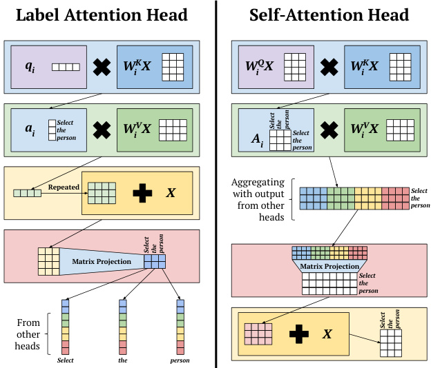
Figure 1: Comparison of the attention head architectures of our proposed Label Attention Layer and a SelfAttention Layer (Vaswani et al., 2017). The matrix $\mathbf{X}$ represents the input sentence “Select the person”.
图 1: 我们提出的标签注意力层 (Label Attention Layer) 与自注意力层 (SelfAttention Layer) (Vaswani et al., 2017) 的注意力头架构对比。矩阵 $\mathbf{X}$ 表示输入句子"Select the person"。
To test our proposed Label Attention Layer, we build upon the parser of Zhou and Zhao (2019) and establish a new state of the art for both constituency and dependency parsing, in both English and Chinese. We also release our pre-trained parsers, as well as our code to encourage experiments with the Label Attention Layer 1.
为验证我们提出的标签注意力层(Label Attention Layer),我们在Zhou和Zhao(2019)的解析器基础上进行改进,在英语和汉语的选区解析与依存解析任务中均取得了新的最优性能。同时开源了预训练解析器及代码,以促进标签注意力层的实验研究[1]。
2 Label Attention Layer
2 标签注意力层
The self-attention mechanism of Vaswani et al. (2017) propagates information between the words of a sentence. Each resulting word representation
Vaswani等人(2017)提出的自注意力机制实现了句子中词语间的信息传递。每个生成的词语表征
Example Input
示例输入
The Label Attention Layer takes word vectors as input (red-contour matrix). In the example sentence, start and end symbols are omitted.
标签注意力层以词向量作为输入(红色轮廓矩阵)。示例句子中省略了起始和结束符号。
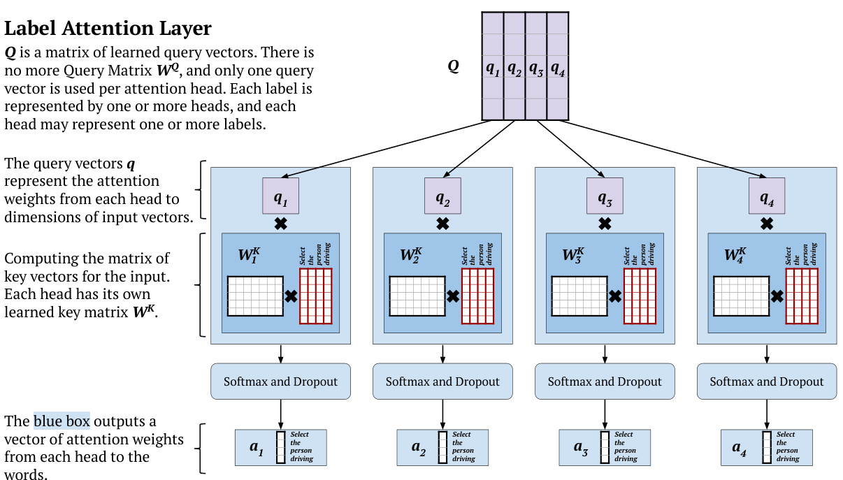
Figure 2: The architecture of the top of our proposed Label Attention Layer. In this figure, the example input sentence is “Select the person driving”.
图 2: 我们提出的标签注意力层 (Label Attention Layer) 顶部架构示意图。图中示例输入句子为"Select the person driving"。
contains its own attention-weighted view of the sentence. We hypothesize that a word representation can be enhanced by including each label’s attention-weighted view of the sentence, on top of the information obtained from self-attention.
包含该句子自身的注意力加权视图。我们假设,在自注意力(self-attention)获得的信息基础上,通过纳入每个标签对句子的注意力加权视图,可以增强词表征。
The Label Attention Layer (LAL) is a novel, modified form of self-attention, where only one query vector is needed per attention head. Each classification label is represented by one or more attention heads, and this allows the model to learn label-specific views of the input sentence. Figure 1 shows a high-level comparison between our Label Attention Layer and self-attention.
标签注意力层 (Label Attention Layer, LAL) 是一种改进的自注意力机制变体,其每个注意力头仅需一个查询向量。每个分类标签由一个或多个注意力头表示,这使得模型能够学习输入句子中与特定标签相关的视图。图 1: 展示了标签注意力层与自注意力机制的高层对比。
We explain the architecture and intuition behind our proposed Label Attention Layer through the example application of parsing.
我们通过解析的示例应用来解释所提出的标签注意力层 (Label Attention Layer) 的架构和设计思路。
Figure 2 shows one of the main differences between our Label Attention mechanism and selfattention: the absence of the Query matrix $\mathbf{W}^{\mathbf{Q}}$ Instead, we have a learned matrix $\mathbf{Q}$ of query vectors representing each head. More formally, for the attention head $i$ and an input matrix $\mathbf{X}$ of word vectors, we compute the corresponding attention weights vector $\mathbf{a}_{i}$ as follows:
图 2: 展示了我们的标签注意力机制与自注意力机制的主要区别之一:移除了查询矩阵 $\mathbf{W}^{\mathbf{Q}}$,取而代之的是表示每个注意力头的可学习查询向量矩阵 $\mathbf{Q}$。更正式地说,对于注意力头 $i$ 和词向量输入矩阵 $\mathbf{X}$,我们按如下方式计算对应的注意力权重向量 $\mathbf{a}_{i}$:
$$
\mathbf{a}{i}=\mathrm{softmax}\left(\frac{\mathbf{q}{i}*\mathbf{K}_{i}}{\sqrt{d}}\right)
$$
$$
\mathbf{a}{i}=\mathrm{softmax}\left(\frac{\mathbf{q}{i}*\mathbf{K}_{i}}{\sqrt{d}}\right)
$$
where $d$ is the dimension of query and key vectors, $\mathbf{K}{i}$ is the matrix of key vectors. Given a learned head-specific key matrix $\mathbf{W}{i}^{K}$ , we compute $\mathbf{K}_{i}$ as:
其中 $d$ 是查询(query)和键(key)向量的维度,$\mathbf{K}{i}$ 是键向量的矩阵。给定一个学习到的头特定键矩阵 $\mathbf{W}{i}^{K}$,我们计算 $\mathbf{K}_{i}$ 为:
$$
\mathbf{K}{i}=\mathbf{W}_{i}^{K}\mathbf{X}
$$
$$
\mathbf{K}{i}=\mathbf{W}_{i}^{K}\mathbf{X}
$$
Each attention head in our Label Attention layer has an attention vector, instead of an attention matrix as in self-attention. Consequently, we do not obtain a matrix of vectors, but a single vector that contains head-specific context information. This context vector corresponds to the green vector in Figure 3. We compute the context vector $\mathbf{c}_{i}$ of head $i$ as follows:
我们的标签注意力层中,每个注意力头都有一个注意力向量,而非自注意力中的注意力矩阵。因此,我们不会得到一个向量矩阵,而是一个包含特定头上下文信息的单一向量。该上下文向量对应图3中的绿色向量。我们按如下方式计算头$i$的上下文向量$\mathbf{c}_{i}$:
$$
\mathbf{c}{i}=\mathbf{a}{i}*\mathbf{V}_{i}
$$
$$
\mathbf{c}{i}=\mathbf{a}{i}*\mathbf{V}_{i}
$$
where $\mathbf{a}{i}$ is the vector of attention weights in Equation 1, and $\mathbf{V}{i}$ is the matrix of value vectors. Given a learned head-specific value matrix $\mathbf{W}{i}^{V}$ , we compute $\mathbf{V}_{i}$ as:
其中 $\mathbf{a}{i}$ 是公式1中的注意力权重向量,$\mathbf{V}{i}$ 是值向量矩阵。给定学习到的特定头值矩阵 $\mathbf{W}{i}^{V}$,我们计算 $\mathbf{V}_{i}$ 如下:
$$
\mathbf{V}{i}=\mathbf{W}_{i}^{V}\mathbf{X}
$$
$$
\mathbf{V}{i}=\mathbf{W}_{i}^{V}\mathbf{X}
$$
The context vector gets added to each individual input vector – making for one residual connection per head, rather one for all heads, as in the yellow box in Figure 3. We project the resulting matrix of word vectors to a lower dimension before normalizing. We then distribute the vectors computed by each label attention head, as shown in Figure 4.
上下文向量会与每个单独的输入向量相加——为每个注意力头形成一个残差连接,而非像图3黄色框所示那样为所有头共用一个。在归一化之前,我们会将生成的词向量矩阵投影到更低维度。随后如图4所示,分配由各标签注意力头计算得到的向量。
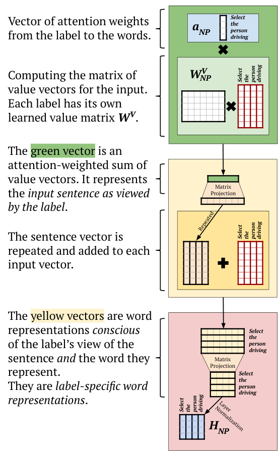
Figure 3: The Value vector computations in our proposed Label Attention Layer.
图 3: 我们提出的标签注意力层中的值向量计算。
We chose to assign as many attention heads to the Label Attention Layer as there are classification labels. As parsing labels (syntactic categories) are related, we did not apply an orthogonality loss to force the heads to learn separate information. We therefore expect an overlap when we match labels to heads. The values from each head are identifiable within the final word representation, as shown in the color-coded vectors in Figure 4.
我们选择为标签注意力层 (Label Attention Layer) 分配与分类标签数量相同的注意力头。由于解析标签 (句法类别) 相关联,我们没有应用正交损失来强制各头学习不同信息。因此,在将标签与头匹配时,我们预期会出现重叠。如图 4 中颜色编码的向量所示,每个头的值在最终词表示中是可识别的。
The activation functions of the position-wise feed-forward layer make it difficult to follow the path of the contributions. Therefore we can remove the position-wise feed-forward layer, and compute the contributions from each label. We provide an example in Figure 6, where the contributions are computed using normalization and averaging. In this case, we are computing the contributions of each head to the span vector. The span representation for “the person” is computed following the method of Gaddy et al. (2018) and Kitaev and Klein (2018). However, forward and backward representations are not formed by splitting the entire word vector at the middle, but rather by splitting each head-specific word vector at the middle.
逐位置前馈层的激活函数使得贡献路径难以追踪。因此我们可以移除逐位置前馈层,转而计算每个标签的贡献值。我们在图6中提供了一个示例,其中贡献值通过归一化和平均化计算得出。此案例中,我们计算的是每个注意力头对span向量的贡献。"the person"的span表征采用Gaddy等人(2018)与Kitaev和Klein(2018)的方法计算。但前向与后向表征并非通过将整个词向量从中部切分形成,而是通过将每个注意力头专属的词向量从中部切分获得。
In the example in Figure 6, we show averaging as one way of computing contributions, other functions, such as softmax, can be used. Another way of interpreting predictions is to look at the head-toword attention distributions, which are the output vectors in the computation in Figure 2.
在图6的示例中,我们展示了平均值计算贡献度的一种方式,也可以使用其他函数(如softmax)。另一种解释预测的方法是观察头词注意力分布,即图2计算过程中的输出向量。
3 Syntactic Parsing Model
3 句法解析模型
3.1 Encoder
3.1 编码器
Our parser is an encoder-decoder model. The encoder has self-attention layers (Vaswani et al., 2017), preceding the Label Attention Layer. We follow the attention partition of Kitaev and Klein (2018), who show that separating content embeddings from position ones improves performance.
我们的解析器采用编码器-解码器架构。编码器包含自注意力层 (Vaswani et al., 2017) 和前置的标签注意力层。我们遵循 Kitaev 和 Klein (2018) 提出的注意力分区方法,该方法证明将内容嵌入与位置嵌入分离能提升模型性能。
Sentences are pre-processed following Zhou and Zhao (2019). Trees are represented using a simplified Head-driven Phrase Structure Grammar (HPSG) (Pollard and Sag, 1994). In Zhou and Zhao (2019), two kinds of span representations are proposed: the division span and the joint span. We choose the joint span representation as it is the best-performing one in their experiments. Figure 5 shows how the example sentence in Figure 2 is represented.
句子预处理遵循Zhou和Zhao (2019)的方法。树结构采用简化的中心词驱动短语结构语法 (HPSG) (Pollard and Sag, 1994) 表示。Zhou和Zhao (2019) 提出了两种跨度表示:分割跨度和联合跨度。我们选择联合跨度表示,因为这是他们实验中表现最佳的方式。图5展示了图2中例句的表示方法。
The token representations for our model are a concatenation of content and position embeddings. The content embeddings are a sum of word and part-of-speech embeddings.
我们模型的Token表示是内容嵌入和位置嵌入的拼接。内容嵌入是词嵌入和词性嵌入的总和。
3.2 Constituency Parsing
3.2 成分句法分析
For constituency parsing, span representations follow the definition of Gaddy et al. (2018) and Kitaev and Klein (2018). For a span starting at the $i$ -th word and ending at the $j$ -th word, the corresponding span vector $s_{i j}$ is computed as:
对于成分句法分析,span表示遵循Gaddy等人(2018) 和Kitaev与Klein(2018) 的定义。对于一个起始于第$i$个单词、结束于第$j$个单词的span,其对应的span向量$s_{ij}$计算方式为:
$$
\mathbf{s_{ij}}=\left[{\overrightarrow{\mathbf{h_{j}}}}-{\overrightarrow{\mathbf{h_{i-1}}}};{\overleftarrow{\mathbf{h_{j+1}}}}-{\overleftarrow{\mathbf{h_{i}}}}\right]
$$
$$
\mathbf{s_{ij}}=\left[{\overrightarrow{\mathbf{h_{j}}}}-{\overrightarrow{\mathbf{h_{i-1}}}};{\overleftarrow{\mathbf{h_{j+1}}}}-{\overleftarrow{\mathbf{h_{i}}}}\right]
$$
where $\overleftarrow{\mathbf{h}{\mathbf{i}}}$ and $\overrightarrow{\mathbf{h}_{\mathbf{i}}}$ are respectively the backward and forward representation of the $i$ -th word obtained by splitting its representation in half. An example of a span representation is shown in the middle of Figure 6.
其中 $\overleftarrow{\mathbf{h}{\mathbf{i}}}$ 和 $\overrightarrow{\mathbf{h}_{\mathbf{i}}}$ 分别是通过将第 $i$ 个词的表示分成两半得到的后向和前向表示。图 6 中间展示了一个跨度表示的示例。
The score vector for the span is obtained by applying a one-layer feed-forward layer:
该跨度的得分向量通过应用单层前馈层获得:
$$
\mathbf{S}(i,j)=\mathbf{W_{2}R e L U}(\mathrm{LN}(\mathbf{W_{1}s_{i j}}+\mathbf{b_{1}}))+\mathbf{b_{2}}
$$
$$
\mathbf{S}(i,j)=\mathbf{W_{2}R e L U}(\mathrm{LN}(\mathbf{W_{1}s_{i j}}+\mathbf{b_{1}}))+\mathbf{b_{2}}
$$
The Position-wise Feed-Forward Layer may optionally be removed.
位置前馈层 (Position-wise Feed-Forward Layer) 可以选择性移除。
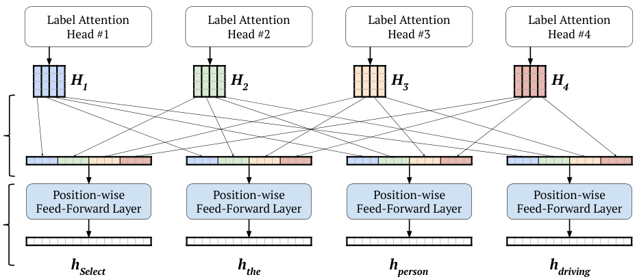
Figure 4: Redistribution of the head-specific word representations to form word vectors by concatenation. We use different colors for each label attention head. The colors show where the head outputs go in the word representations. We do not use colors for the vectors resulting from the position-wise feed-forward layer, as the head-specific information moved.
图 4: 通过拼接重新分配头部特定词表征以形成词向量。我们为每个标签注意力头使用不同颜色,颜色表明头部输出在词表征中的去向。由于位置前馈层移动了头部特定信息,因此未对由此产生的向量着色。
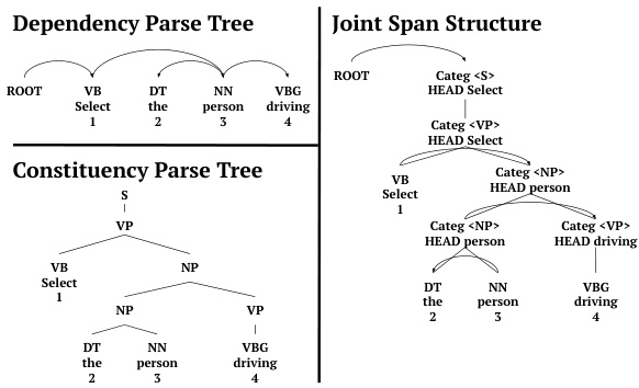
Figure 5: Parsing representations of the example sentence in Figure 2.
图 5: 图 2 中例句的解析表示。
where LN is Layer Normalization, and $\mathbf{W_{1}},\mathbf{W_{2}}$ , $\mathbf{b_{1}}$ and $\mathbf{b_{2}}$ are learned parameters. For the $l$ -th syntactic category, the corresponding score $s(i,j,l)$ is then the $l$ -th value in the $\mathbf{S}(i,j)$ vector.
其中 LN 表示层归一化 (Layer Normalization),$\mathbf{W_{1}},\mathbf{W_{2}}$、$\mathbf{b_{1}}$ 和 $\mathbf{b_{2}}$ 为可学习参数。对于第 $l$ 个句法类别,其对应得分 $s(i,j,l)$ 即为向量 $\mathbf{S}(i,j)$ 中的第 $l$ 个值。
Consequently, the score of a constituency parse tree $T$ is the sum of all of the scores of its spans and their syntactic categories:
因此,选区解析树 $T$ 的分数是其所有跨度和句法类别分数的总和:
$$
s(T)=\sum_{(i,j,l)\in T}s(i,j,l)
$$
$$
s(T)=\sum_{(i,j,l)\in T}s(i,j,l)
$$
We then use a CKY-style algorithm (Stern et al., 2017; Gaddy et al., 2018) to find the highest scoring tree $\hat{T}$ . The model is trained to find the correct parse tree $T^{*}$ , such that for all trees $T$ , the following margin constraint is satisfied:
我们随后采用CKY风格算法 (Stern et al., 2017; Gaddy et al., 2018) 来寻找最高分树 $\hat{T}$ 。该模型被训练用于寻找正确解析树 $T^{*}$ ,使得对于所有树 $T$ ,满足以下边界约束条件:
$$
s(T^{})\geq s(T)+\Delta(T,T^{*})
$$
$$
s(T^{})\geq s(T)+\Delta(T,T^{*})
$$
where $\Delta$ is the Hamming loss on labeled spans. The corresponding loss function is the hinge loss:
其中 $\Delta$ 是标注跨度的汉明损失 (Hamming loss)。对应的损失函数是合页损失 (hinge loss):
$$
L_{c}=\operatorname*{max}\left(0,\operatorname*{max}_{T}[s(T)+\Delta(T,T^{})]-s(T^{*})\right)
$$
$$
L_{c}=\operatorname*{max}\left(0,\operatorname*{max}_{T}[s(T)+\Delta(T,T^{})]-s(T^{*})\right)
$$
3.3 Dependency Parsing
3.3 依存句法分析
We use the biaffine attention mechanism (Dozat and Manning, 2016) to compute a probability distribution for the dependency head of each word. The child-parent score $\alpha_{i j}$ for the $j$ -th word to be the head of the $i$ -th word is:
我们使用双仿射注意力机制 (biaffine attention mechanism) [20] 来计算每个词语依存头的概率分布。第$j$个词作为第$i$个词依存头的子父得分$\alpha_{ij}$为:
$$
\alpha_{i j}=\mathbf{h_{i}^{(d)}}^{T}\mathbf{W}\mathbf{h_{j}^{(h)}}+\mathbf{U}^{T}\mathbf{h_{i}^{(d)}}+\mathbf{V}^{T}\mathbf{h_{j}^{(h)}}+b
$$
$$
\alpha_{i j}=\mathbf{h_{i}^{(d)}}^{T}\mathbf{W}\mathbf{h_{j}^{(h)}}+\mathbf{U}^{T}\mathbf{h_{i}^{(d)}}+\mathbf{V}^{T}\mathbf{h_{j}^{(h)}}+b
$$
where $\mathbf{h_{i}^{(d)}}$ is the dependent representation of the $i$ -th word obtained by putting its representation $\mathbf{h}{\mathbf{i}}$ through a one-layer perceptron. Likewise, $\mathbf{h_{j}^{(h)}}$ is the head representation of the $j$ -th word obtained by putting its representation $\mathbf{h}_{\mathbf{j}}$ through a separate one-layer perceptron. The matrices W, U and $\mathbf{V}$ are learned parameters.
其中 $\mathbf{h_{i}^{(d)}}$ 是通过将第 $i$ 个单词的表示 $\mathbf{h}{\mathbf{i}}$ 输入单层感知机得到的依赖表示。类似地,$\mathbf{h_{j}^{(h)}}$ 是通过将第 $j$ 个单词的表示 $\mathbf{h}_{\mathbf{j}}$ 输入另一个单层感知机得到的主干表示。矩阵 W、U 和 $\mathbf{V}$ 是待学习的参数。
The model trains on dependency parsing by minimizing the negative likelihood of the correct dependency tree. The loss function is cross-entropy:
模型通过最小化正确依存树的负对数似然来进行依存解析训练。损失函数为交叉熵:
$$
L_{d}=-\mathrm{log}\left(P\left(h_{i}|d_{i}\right)P\left(l_{i}|d_{i},h_{i}\right)\right)
$$
$$
L_{d}=-\mathrm{log}\left(P\left(h_{i}|d_{i}\right)P\left(l_{i}|d_{i},h_{i}\right)\right)
$$
where $h_{i}$ is the correct head for dependent $d_{i}$ , $P\left(h_{i}|d_{i}\right)$ is the probability that $h_{i}$ is the head of $d_{i}$ , and $P\left({{l}{i}}|{{d}{i}},{{h}{i}}\right)$ is the probability of the correct dependency label $l_{i}$ for the child-parent pair $(d_{i},h_{i})$ .
其中 $h_{i}$ 是依存词 $d_{i}$ 的正确中心词,$P\left(h_{i}|d_{i}\right)$ 表示 $h_{i}$ 作为 $d_{i}$ 中心词的概率,$P\left({{l}{i}}|{{d}{i}},{{h}{i}}\right)$ 表示子-父对 $(d_{i},h_{i})$ 获得正确依存标签 $l_{i}$ 的概率。
Computing Head Contributions
计算头部贡献
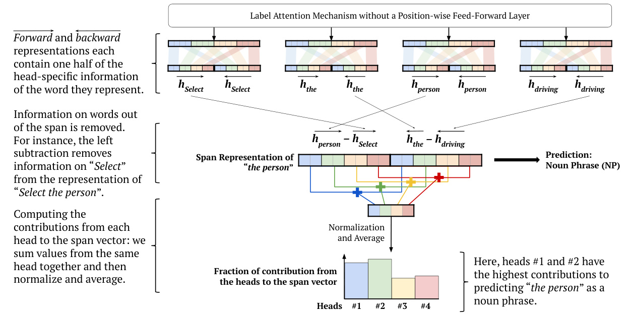
Figure 6: If we remove the position-wise feed-forward layer, we can compute the contributions from each label attention head to the span representation, and thus interpret head contributions. This illustrative example follows the label color scheme in Figure 4.
图 6: 如果移除位置前馈层,我们可以计算每个标签注意力头对跨度表示的贡献,从而解释头的贡献。此示例遵循图4中的标签配色方案。
3.4 Decoder
3.4 解码器
The model jointly trains on constituency and dependency parsing by minimizing the sum of the constituency and dependency losses:
该模型通过最小化成分句法分析和依存句法分析的损失之和进行联合训练:
$$
L=L_{c}+L_{d}
$$
$$
L=L_{c}+L_{d}
$$
The decoder is a CKY-style (Kasami, 1966; Younger, 1967; Cocke, 1969; Stern et al., 2017) algorithm, modified by Zhou and Zhao (2019) to include dependency scores.
解码器采用CKY风格算法 (Kasami, 1966; Younger, 1967; Cocke, 1969; Stern et al., 2017),并由Zhou和Zhao (2019) 改进以包含依存分数。
4 Experiments
4 实验
We evaluate our model on the English Penn Treebank (PTB) (Marcus et al., 1993) and on the Chinese Treebank (CTB) (Xue et al., 2005). We use the Stanford tagger (Toutanova et al., 2003) to pre- dict part-of-speech tags and follow standard data splits.
我们在英文宾州树库 (PTB) (Marcus等人, 1993) 和中文树库 (CTB) (Xue等人, 2005) 上评估模型。使用斯坦福标注器 (Toutanova等人, 2003) 预测词性标签,并遵循标准数据划分。
Following standard practice, we use the EVALB algorithm (Sekine and Collins, 1997) for constituency parsing, and report results without punctuation for dependency parsing.
按照标准做法,我们使用EVALB算法 (Sekine and Collins, 1997) 进行成分句法分析,并报告不带标点的依存句法分析结果。
4.1Setup
4.1 设置
In our English-language experiments, the Label Attention Layer has 112 heads: one per syntactic category. However, this is an experimental choice, as the model is not designed to have a one-on-one corresponden ce between attention heads and syntactic categories. The Chinese Treebank is a smaller dataset, and therefore we use 64 heads in Chineselanguage experiments, even though the number of Chinese syntactic categories is much higher. For both languages, the query, key and value vectors, as well as the output vectors of each label attention head, have 128 dimensions, as determined through short parameter-tuning experiments. For the dependency and span scores, we use the same hyperparameters as Zhou and Zhao (2019). We use the large cased pre-trained XLNet (Yang et al., 2019) as our embedding model for our English-language experiments, and a base pre-trained BERT (Devlin et al., 2018) for Chinese.
在我们的英语实验中,标签注意力层 (Label Attention Layer) 设有112个头 (heads) :每个句法类别对应一个。然而,这只是实验设计的选择,因为该模型并未要求注意力头与句法类别必须一一对应。由于中文树库 (Chinese Treebank) 数据集规模较小,我们在中文实验中仅使用64个头,尽管中文的句法类别数量要多得多。两种语言的查询 (query) 、键 (key) 、值 (value) 向量以及每个标签注意力头的输出向量均设定为128维,这是通过简短的参数调优实验确定的。对于依存关系和跨度评分,我们采用了与Zhou和Zhao (2019) 相同的超参数。英语实验使用大写的预训练XLNet (Yang等, 2019) 作为嵌入模型,中文实验则采用基础版预训练BERT (Devlin等, 2018) 。
We try English-language parsers with 2, 3, 4, 6, 8, 12 and 16 self-attention layers. Our parsers with 3 and 4 self-attention layers are tied in terms of F1 score, and sum of UAS and LAS scores. The results of our fine-tuning experiments are in the appendix. We decide to use 3 self-attention layers for all the following experiments, for lower computational complexity.
我们尝试了具有2、3、4、6、8、12和16个自注意力层 (self-attention layers) 的英语解析器。其中3层和4层结构的解析器在F1分数、UAS与LAS分数总和上表现相当。微调实验的具体结果见附录。考虑到计算复杂度,后续实验均采用3层自注意力结构。
4.2 Ablation Study
4.2 消融实验
As shown in Figure 6, we can compute the contributions from label attention heads only if there is no position-wise feed-forward layer. Residual dropout in self-attention applies to the aggregated outputs from all heads. In label attention, residual dropout applies separately to the output of each head, and therefore can cancel out parts of the head contributions. We investigate the impact of removing these two components from the LAL.
如图 6 所示,我们只能在不存在逐位置前馈层的情况下计算标签注意力头 (label attention heads) 的贡献。自注意力中的残差丢弃 (residual dropout) 适用于所有头的聚合输出。在标签注意力中,残差丢弃会分别应用于每个头的输出,因此可能抵消部分头的贡献。我们研究了从 LAL 中移除这两个组件的影响。
Table 1: Results on the PTB test set of the ablation study on the Position-wise Feed-forward Layer (PFL) and Residual Dropout (RD) of the Label Attention Layer.
表 1: 在PTB测试集上对标签注意力层的位置前馈层(PFL)和残差丢弃(RD)进行的消融研究结果
| PFL | RD | Prec. | Recall | F1 | UAS | LAS |
|---|---|---|---|---|---|---|
| Yes No Yes | Yes Yes No | 96.47 96.51 96.53 | 96.20 96.15 96.24 | 96.34 96.33 96.38 | 97.33 97.25 97.42 | 96.29 96.11 96.26 |
Table 2: Results on the PTB test set of the ablation study on the Query Vectors (QV) and Concatenation (Conc.) parts of the Label Attention Layer.
表 2: 标签注意力层中查询向量(QV)和拼接(Conc.)部分消融实验在PTB测试集上的结果
| QV | Conc. | Prec. | Recall | F1 | UAS | LAS |
|---|---|---|---|---|---|---|
| Yes No Yes No | Yes Yes No No | 96.53 96.43 96.30 96.30 | 96.24 96.03 96.10 96.06 | 96.38 96.23 96.20 96.18 | 97.42 97.25 97.23 97.26 | 96.26 96.12 96.15 96.17 |
We show the results on the PTB dataset of our ablation study on Residual Dropout and Positionwise Feed-forward Layer in Table 1. We use the same residual dropout probability as Zhou and Zhao (2019). When removing the position-wise feed-forward layer and keeping residual dropout, we observe only a slight decrease in overall performance, as shown in the second row. There is therefore no significant loss in performance in exchange for the interpret ability of the attention heads.
我们在表1中展示了在PTB数据集上对残差丢弃(Residual Dropout)和逐位置前馈层(Positionwise Feed-forward Layer)进行消融研究的结果。我们采用了与Zhou和Zhao (2019)相同的残差丢弃概率。如第二行所示,当移除逐位置前馈层并保留残差丢弃时,我们仅观察到整体性能的轻微下降。因此,用注意力头的可解释性换取性能并不会造成显著损失。
We observe an increase in performance when removing residual dropout only. This suggests that all head contributions are important for performance, and that we were likely over-regularizing.
我们观察到仅移除残差丢弃 (residual dropout) 时性能有所提升。这表明所有注意力头 (head) 的贡献对性能都很重要,而我们之前可能过度正则化了。
Finally, removing both position-wise feedforward layer and residual dropout brings about a noticeable decrease in performance. We continue our experiments without residual dropout.
最后,同时移除位置前馈层和残差丢弃会导致性能显著下降。我们在后续实验中不再使用残差丢弃。
4.3 Comparison with Self-Attention
4.3 与自注意力机制的对比
The two main architecture novelties of our proposed Label Attention Layer are the learned Query Vectors that represent labels and replace the Query Matrix in self-attention, and the Concatenation of the outputs of each attention head that replaces the Matrix Projection in self-attention.
我们提出的标签注意力层 (Label Attention Layer) 的两大架构创新在于:用代表标签的可学习查询向量 (Query Vectors) 取代自注意力中的查询矩阵 (Query Matrix),以及通过拼接各注意力头输出取代自注意力中的矩阵投影 (Matrix Projection)。
In this subsection, we evaluate whether our proposed architecture novelties bring about performance improvements. To this end, we establish an ablation study to compare Label Attention with Self-Attention. We propose three additional model architectures based on our best parser: all models have 3 self-attention layers and a modified Label Attention Layer with 112 attention heads. The three modified Label Attention Layers are as follows: (1) Ablation of Query Vectors: the first model (left of Figure 7) has a Query Matrix like self-attention, and concatenates attention head outputs like Label Attention. (2) Ablation of Concatenation: the second model (right of Figure 7) has a Query Vector like Label Attention, and applies matrix projection to all head outputs like self-attention. (3) Ablation of Query Vectors and Concatenation: the third model (right of Figure 1) has a 112-head self-attention layer.
在本小节中,我们评估所提出的架构创新是否带来性能提升。为此,我们建立消融实验来比较标签注意力 (Label Attention) 与自注意力 (Self-Attention) 的差异。基于最佳解析器,我们提出三种附加模型架构:所有模型均包含3层自注意力层和1个改进的标签注意力层(含112个注意力头)。三种改进的标签注意力层配置如下:(1) 查询向量消融:第一个模型 (图7左) 采用类似自注意力的查询矩阵 (Query Matrix),但像标签注意力那样拼接注意力头输出;(2) 拼接操作消融:第二个模型 (图7右) 采用类似标签注意力的查询向量 (Query Vector),但像自注意力那样对所有头输出进行矩阵投影;(3) 双重消融:第三个模型 (图1右) 直接使用112头的标准自注意力层。

Figure 7: The two hybrid parser architectures for the ablation study on the Label Attention Layer’s Query Vectors and Concatenation.
图 7: 用于标签注意力层查询向量与连接消融研究的两种混合解析器架构。
The results of our experiments are in Table 2. The second row shows that, even though query matrices employ more parameters and computation than query vectors, replacing query vectors by query matrices decreases performance. There is a similar decrease in performance when removing concatenation as well, as shown in the last row. This suggests that our Label Attention Layer learns meaningful representations in its query vectors, and that head-to-word attention distributions are more helpful to performance than query matrices and word-to-word attention distributions.
我们的实验结果如表2所示。第二行显示,尽管查询矩阵比查询向量使用了更多参数和计算量,但用查询矩阵替换查询向量会降低性能。如最后一行所示,移除连接操作同样会导致性能下降。这表明我们的标签注意力层在其查询向量中学习了有意义的表征,且头到词注意力分布比查询矩阵和词到词注意力分布对性能更有帮助。
In self-attention, the output vector is a matrix projection of the concatenation of head outputs. In Label Attention, the head outputs do not interact through matrix projection, but are concatenated. The third and fourth rows of Table 2 show that there is a significant decrease in performance when replacing concatenation with the matrix projection. This decrease suggests that the model benefits from having one residual connection per attention head, rather than one for all attention heads, and from separating head-specific information in word represent at ions. In particular, the last row shows that replacing our LAL with a self-attention layer with an equal number of attention heads decreases performance: the difference between the performance of the first row and the last row is due to the Label Attention Layer’s architecture novelties.
在自注意力机制中,输出向量是多个注意力头输出的矩阵投影拼接。而在标签注意力机制中,注意力头的输出不通过矩阵投影交互,而是直接拼接。表2的第三行和第四行显示:当用矩阵投影替代拼接操作时,模型性能显著下降。这一现象表明,模型更受益于每个注意力头拥有独立的残差连接(而非所有注意力头共享一个残差连接),以及在词表征中保持各注意力头信息的独立性。特别值得注意的是,最后一行数据显示:用具有同等数量注意力头的自注意力层替代我们的LAL(标签注意力层)会导致性能下降——首行与末行之间的性能差异正是源于标签注意力层的架构创新。
Table 3: Constituency Parsing on PTB & CTB test sets.
表 3: PTB 和 CTB 测试集上的选区解析结果。
| 模型 | 英语 LR | 英语 LP | 英语 F1 | 中文 LR | 中文 LP | 中文 F1 |
|---|---|---|---|---|---|---|
| Shenetal.(2018) Fried and Klein (2018) Teng and Zhang (2018) Vaswani et al.(2017) Dyer et al. (2016) | 92.0 92.2 | 91.7 92.5 | 91.8 92.2 92.4 92.7 93.3 | 86.6 86.6 | 86.4 88.0 | 86.5 87.0 87.3 |
| Kuncoro et al.(2017) | 93.6 | 84.6 | ||||
| Charniaket al.(2016) | 93.8 | |||||
| Liu and Zhang (2017b) | 91.3 | |||||
| 92.1 | 91.7 | 85.9 | 85.2 | 85.5 | ||
| Liu and Zhang (2017a) | ||||||
| Suzukietal.(2018) | 94.2 | 86.1 | ||||
| Takase et al.(2018) | 94.32 | |||||
| 94.47 | ||||||
| Fried et al.(2017) | 94.66 | |||||
| Kitaev andKlein(2018) | 94.85 | 95.40 | 95.13 | |||
| Kitaevetal.(2018) | 95.51 | 96.03 | 95.77 | 91.55 | 91.96 | 91.75 |
| Zhou and Zhao (2019) (BERT) | 95.70 | 95.98 | 95.84 | 92.03 | 92.33 | 92.18 |
| ZhouandZhao (2019) | ||||||
| 96.21 | 96.46 | 96.33 | ||||
| (XLNet) Our work | 96.24 |
4.4 English and Chinese Results
4.4 英文与中文结果
Table 4: Dependency Parsing on PTB & CTB test sets.
表 4: PTB和CTB测试集上的依存句法分析结果。
| 模型 | 英语 | 汉语 |
|---|---|---|
| UAS | LAS | |
| Kuncoro et al.(2016) Li et al. (2018) | 94.26 | 92.06 92.08 |
| Ma and Hovy (2017) Dozat and Manning (2016) ChoeandCharniak(2016) Ma et al. (2018) | 94.11 94.88 | 92.98 |
| 95.74 | 94.08 | |
| 95.9 | 94.1 | |
| 95.87 | 94.19 | |
| 95.97 | 94.31 | |
| 96.04 | 94.43 | |
| Rodriguez (2019) Kuncoro et al.(2017) | 95.8 | 94.6 |
| Clark et al. (2018) Wang et al. (2018) | 96.61 | 95.02 |
| Zhou andZhao (2019)(BERT) | 96.35 | 95.25 |
| Zhou and Zhao(2019) (XLNet) Our work 97.42 | 97.00 97.20 | 95.43 95.72 |
Our best-performing English-language parser does not have residual dropout, but has a position-wise feed-forward layer. We train Chinese-language parsers using the same configuration. The Chinese Treebank has two data splits for the training, development and testing sets: one for Constituency (Liu and Zhang, 2017b) and one for Dependency parsing (Zhang and Clark, 2008).
我们表现最佳的英语解析器没有使用残差丢弃 (residual dropout),但包含逐位置前馈层。中文解析器采用相同配置进行训练。中文树库 (Chinese Treebank) 为训练集、开发集和测试集提供两种数据划分:一种用于成分句法分析 (Liu and Zhang, 2017b),另一种用于依存句法分析 (Zhang and Clark, 2008)。
Finally, we compare our results with the state of the art in constituency and dependency parsing in both English and Chinese. We show our Constituency Parsing results in Table 3, and our Dependency Parsing results in Table 4. Our LAL parser establishes new state-of-the-art results in both languages, improving significantly in dependency parsing.
最后,我们将结果与当前英语和汉语中最先进的成分句法分析和依存句法分析进行比较。成分句法分析结果如表 3 所示,依存句法分析结果如表 4 所示。我们的 LAL 解析器在两种语言中都达到了新的最先进水平,在依存句法分析方面有显著提升。
4.5 Interpreting Head Contributions
4.5 解读注意力头贡献
We follow the method in Figure 6 to identify which attention heads contribute to predictions. We collect the span vectors from the Penn Treebank test set, and we use our LAL parser with no positionwise feed-forward layer for predictions.
我们遵循图6中的方法来识别哪些注意力头对预测有贡献。我们从Penn Treebank测试集中收集跨度向量,并使用不带位置前馈层的LAL解析器进行预测。
Figure 8 displays the bar charts for the three most common syntactic categories: Noun Phrases (NP), Verb Phrases (VP) and Sentences (S). We notice several heads explain each predicted category.
图 8: 展示了三种最常见句法类别的柱状图:名词短语(NP)、动词短语(VP)和句子(S)。我们注意到多个注意力头分别解释了每个预测类别。
We collect statistics about the top-contributing heads for each predicted category. Out of the NP spans, $44.9%$ get their top contribution from head 35, $13.0%$ from head 47, and $7.3%$ from head 0. The top-contributing heads for VP spans are heads 31 $(61.1%)$ , 111 $(13.2%)$ , and 71 $(7.5%)$ . As for S spans, the top-contributing heads are 52 $(48.6%)$ , 31 $(22.8%)$ , 35 $(6.9%)$ , and 111 $(5.2%)$ . We see that S spans share top-contributing heads with VP spans (heads 31 and 111), and NP spans (head 35). The similarities reflect the relations between the syntactic categories. In this case, our Label Attention Layer learned the rule ${\bf S}\rightarrow{\bf N P}$ VP.
我们统计了每个预测类别中贡献最大的注意力头。在名词短语(NP)片段中,44.9%的最大贡献来自头35,13.0%来自头47,7.3%来自头0。动词短语(VP)片段的最大贡献头为头31 (61.1%)、头111 (13.2%)和头71 (7.5%)。对于句子(S)片段,最大贡献头是头52 (48.6%)、头31 (22.8%)、头35 (6.9%)和头111 (5.2%)。我们发现S片段与VP片段(头31和头111)及NP片段(头35)共享最大贡献头。这种相似性反映了句法类别之间的关系。在本例中,我们的标签注意力层学习到了规则${\bf S}\rightarrow{\bf N P}$ VP。
Moreover, the top-contributing heads for PP spans are 35 $(29.6%)$ , 31 $(26.7%)$ , 111 $(10.3%)$ , and 47 $(9.4%)$ : they are equally split between NP spans (heads 35 and 47) and VP spans (heads 31 and 111). Here, the LAL has learned that both verb and noun phrases can contain preposition phrases.
此外,对介词短语(PP)跨度贡献最大的注意力头是35 $(29.6%)$、31 $(26.7%)$、111 $(10.3%)$和47 $(9.4%)$:它们平均分配在名词短语(NP)跨度(头35和47)和动词短语(VP)跨度(头31和111)之间。这表明LAL已学会动词短语和名词短语都可以包含介词短语。
We see that head 52 is unique to S spans. Actually, $64.7%$ of spans with head 52 as the highest contribution are S spans. Therefore our model has learned to represent the label S using head 52.
我们发现头52是S跨度的独特特征。实际上,以头52作为最高贡献的跨度中有64.7%是S跨度。因此,我们的模型学会了使用头52来表示标签S。
All of the aforementioned heads are represented in Figure 8. We see that heads that have low contributions for NP spans, peak in contribution for VP spans (heads 31, 71 and 111), and vice-versa (heads 0, 35 and 47). Moreover, NP spans do not share any top-contributing head with VP spans. This shows that our parser has also learned the differences between dissimilar syntactic categories.
上述所有注意力头均在图8中展示。我们可以观察到,对名词短语(NP)跨度贡献较低的注意力头(如头31、71和111)在动词短语(VP)跨度中贡献达到峰值,反之亦然(如头0、35和47)。此外,NP跨度与VP跨度之间不存在任何共享的高贡献注意力头。这表明我们的解析器已经学会了区分不同句法范畴之间的差异。

Figure 8: Average contribution of select heads to span vectors with different predicted syntactic categories.
图 8: 所选注意力头对不同预测句法类别的span向量的平均贡献。
4.6 Error Analysis
4.6 误差分析
Head-to-Word Attention. We analyze prediction errors from the PTB test set. One example is the span “Fed Ready to Inject Big Funds”, predicted as NP but labelled as S. We trace back the attention weights for each word, and find that, out of the 9 top-contributing heads, only 2 focus their attention on the root verb of the sentence (Inject), while 4 focus on a noun (Funds), resulting in a noun phrase prediction. We notice similar patterns in other wrongly predicted spans, suggesting that forcing the attention distribution to focus on a relevant word might correct these errors.
词对词注意力机制分析。我们解析了PTB测试集中的预测错误案例,例如片段"Fed Ready to Inject Big Funds"被预测为NP(名词短语)却标注为S(句子)。通过追溯每个词的注意力权重发现:在贡献度最高的9个注意力头中,仅2个头聚焦于句子核心动词(Inject),却有4个头集中于名词(Funds),导致模型输出名词短语预测。在其他错误预测片段中观察到类似模式,这表明强制调整注意力分布至相关关键词可能修正此类错误。
Top-Contributing Heads. We analyze wrongly predicted spans by their true category. Out of the 53 spans labelled as NP but not predicted as such, we still see the top-contributing head for 36 of them is either head 35 or 47, both top-contributing heads of spans predicted as NP. Likewise, for the 193 spans labelled as S but not predicted as such, the top-contributing head of 141 of them is one of the four top-contributing heads for spans predicted as S. This suggests that a stronger prediction link to the label attention heads, through a loss function for instance, may increase the performance.
贡献最大的注意力头。我们按真实类别分析错误预测的片段。在53个被标注为NP但未预测为NP的片段中,仍有36个片段的最大贡献头是头35或47(这两个头也是预测为NP片段的主要贡献头)。同样,在193个被标注为S但未预测为S的片段中,有141个片段的最大贡献头属于预测为S片段的四个主要贡献头之一。这表明,通过损失函数等方式加强预测与标签注意力头之间的关联,可能会提升模型性能。
5 Related Work
5 相关工作
Since their introduction in Machine Translation, attention mechanisms (Bahdanau et al., 2014; Luong et al., 2015) have been extended to other tasks, such as text classification (Yang et al., 2016), natural language inference (Chen et al., 2016) and language modeling (Salton et al., 2017).
自应用于机器翻译以来,注意力机制 (Bahdanau et al., 2014; Luong et al., 2015) 已被扩展到其他任务,如文本分类 (Yang et al., 2016)、自然语言推理 (Chen et al., 2016) 和语言建模 (Salton et al., 2017)。
Self-attention and transformer architectures (Vaswani et al., 2017) are now the state of the art in language understanding (Devlin et al., 2018; Yang et al., 2019), extractive sum mari z ation (Liu, 2019), semantic role labeling (Strubell et al., 2018) and machine translation for low-resource languages (Rikters, 2018; Rikters et al., 2018).
自注意力机制 (self-attention) 和 Transformer 架构 (Vaswani et al., 2017) 现已成为语言理解 (Devlin et al., 2018; Yang et al., 2019)、抽取式摘要 (Liu, 2019)、语义角色标注 (Strubell et al., 2018) 以及低资源语言机器翻译 (Rikters, 2018; Rikters et al., 2018) 领域的最先进技术。
While attention mechanisms can provide explanations for model predictions, Serrano and Smith (2019) challenge that assumption and find that attention weights only noisily predict overall importance with regard to the model. Jain and Wallace (2019) find that attention distributions rarely correlate with feature importance weights. However, Wiegreffe and Pinter (2019) show through alternative tests that prior work does not discredit the usefulness of attention for interpret ability.
虽然注意力机制能为模型预测提供解释,但Serrano和Smith (2019) 对这一假设提出质疑,发现注意力权重仅能嘈杂地预测模型整体重要性。Jain和Wallace (2019) 指出注意力分布很少与特征重要性权重相关。然而,Wiegreffe和Pinter (2019) 通过替代性实验证明,先前研究并未否定注意力对可解释性的实用价值。
Xiao et al. (2019) introduce the Label-Specific Attention Network (LSAN) for multi-label document classification. They use label descriptions to compute attention scores for words, and follow the self-attention of Lin et al. (2017). Cui and Zhang (2019) introduce a Label Attention Inference Layer for sequence labeling, which uses the self-attention of Vaswani et al. (2017). In this case, the key and value vectors are learned label embeddings, and the query vectors are hidden vectors obtained from a Bi-LSTM encoder. Our work is unrelated to these two papers, as they were published towards the end of our project.
Xiao等人 (2019) 提出了用于多标签文档分类的标签特定注意力网络 (LSAN)。他们利用标签描述计算词语的注意力分数,并沿用了Lin等人 (2017) 提出的自注意力机制。Cui和Zhang (2019) 则为序列标注任务设计了标签注意力推理层,该模块采用Vaswani等人 (2017) 的自注意力架构,其中键向量和值向量是可学习的标签嵌入,查询向量则来自Bi-LSTM编码器生成的隐藏向量。我们的工作与这两篇论文无关,因为它们发表于本项目临近结束时。
6 Conclusions
6 结论
In this paper, we introduce a new form of selfattention: the Label Attention Layer. In our proposed architecture, attention heads represent labels. We incorporate our Label Attention Layer into the HPSG parser (Zhou and Zhao, 2019) and obtain new state-of-the-art results on the Penn Treebank and Chinese Treebank. In English, our results show 96.38 F1 for constituency parsing, and 97.42 UAS and $96.26~\mathrm{LAS}$ for dependency parsing. In Chinese, our model achieves 92.64 F1, 94.56 UAS and 89.28 LAS.
本文介绍了一种新型自注意力机制:标签注意力层 (Label Attention Layer)。在所提出的架构中,注意力头 (attention heads) 代表标签。我们将标签注意力层整合到HPSG解析器 (Zhou and Zhao, 2019) 中,在宾州树库 (Penn Treebank) 和中文树库 (Chinese Treebank) 上取得了新的最先进结果。在英语任务中,我们的模型在成分句法分析上获得96.38 F1值,在依存句法分析上获得97.42 UAS和$96.26~\mathrm{LAS}$;在中文任务中,模型取得了92.64 F1值、94.56 UAS和89.28 LAS值。
We perform ablation studies that show the Query Vector learned by our Label Attention Layer outperform the self-attention Query Matrix. Since we have only one learned vector as query, rather than a matrix, we can significantly reduce the number of parameters per attention head. Finally, our Label Attention heads learn the relations between the syntactic categories, as we show by computing contributions from each attention head to span vectors. We show how the heads also help to analyze prediction errors, and suggest methods to correct them.
我们进行的消融研究表明,标签注意力层(Label Attention Layer)学习到的查询向量(Query Vector)优于自注意力查询矩阵(self-attention Query Matrix)。由于我们仅使用一个学习到的向量作为查询(而非矩阵),可显著减少每个注意力头的参数量。最后,通过计算各注意力头对跨度向量(span vectors)的贡献度,我们发现标签注意力头能够学习句法类别间的关系。实验还展示了这些注意力头如何辅助分析预测错误,并提出了相应的修正方法。
A Additional Experiment Results
A 补充实验结果
We report experiment results for hyper parameter tuning based on the number of self-attention layers in Table 5.
我们在表5中报告了基于自注意力层数的超参数调优实验结果。
Table 5: Performance on the Penn Treebank test set of our LAL parser according to the number of self-attention layers. All parsers here include the Position-wise Feed-forward Layer and Residual Dropout.
表 5: 我们的 LAL 解析器在 Penn Treebank 测试集上的性能表现,按自注意力层数划分。所有解析器均包含位置前馈层和残差丢弃。
| 自注意力层数 | 精确率 | 召回率 | F1值 | UAS | LAS |
|---|---|---|---|---|---|
| 2 | 96.23 | 96.03 | 96.13 | 97.16 | 96.09 |
| 3 | 96.47 | 96.20 | 96.34 | 97.33 | 96.29 |
| 4 | 96.52 | 96.15 | 96.34 | 97.39 | 96.23 |
| 6 | 96.48 | 96.09 | 96.29 | 97.30 | 96.16 |
| 8 | 96.43 | 96.09 | 96.26 | 97.33 | 96.15 |
| 12 | 96.27 | 96.06 | 96.16 | 97.24 | 96.14 |
| 16 | 96.38 | 96.02 | 96.20 | 97.32 | 96.11 |