Optimization of Graph Neural Networks with Natural Gradient Descent
基于自然梯度下降的图神经网络优化
Abstract
摘要
In this work, we propose to employ information-geometric tools to optimize a graph neural network architecture such as the graph convolutional networks. More specifically, we develop optimization algorithms for the graph-based semi-supervised learning by employing the natural gradient information in the optimization process. This allows us to efficiently exploit the geometry of the underlying statistical model or parameter space for optimization and inference. To the best of our knowledge, this is the first work that has utilized the natural gradient for the optimization of graph neural networks that can be extended to other semi-supervised problems. Efficient computations algorithms are developed and extensive numerical studies are conducted to demonstrate the superior performance of our algorithms over existing algorithms such as ADAM and SGD.
在本研究中,我们提出运用信息几何工具来优化图神经网络架构(如Graph Convolutional Networks)。具体而言,我们通过在优化过程中引入自然梯度信息,开发了基于图的半监督学习优化算法。这种方法能高效利用底层统计模型或参数空间的几何结构进行优化与推断。据我们所知,这是首个将自然梯度应用于图神经网络优化的研究,该框架可扩展至其他半监督学习问题。我们开发了高效的计算算法,并通过大量数值实验证明:相比ADAM、SGD等现有算法,新算法具有显著性能优势。
Index Terms
索引术语
Graph neural network, Fisher information, natural gradient descent, network data.
图神经网络 (Graph Neural Network)、费雪信息 (Fisher information)、自然梯度下降 (Natural Gradient Descent)、网络数据 (Network Data)
I. INTRODUCTION
I. 引言
In machine learning, the cost function is mostly evaluated using labeled samples that are not easy to collect. Semi-supervised learning tries to find a better model by using unlabeled samples. Most of the semi-supervised methods are based on a graph representation on (transformed) samples and labels [11]. For example, augmentation methods create a new graph in which original and augmented samples are connected. Graphs, as datasets with linked samples, have been the center of attention in semi-supervised learning. Graph Neural Network (GNN), initially proposed to capture graph representations in neural networks [20], have been used for semisupervised learning in a variety of problems like node classification, link predictions, and so on. The goal of each GNN layer is to transform features while considering the graph structure by aggregating information from connected or neighboring nodes. When there is only one graph, the goal of node classification becomes predicting node labels in a graph while only a portion of node labels are available (even though the model might have access to the features of all nodes). Inspired by the advance of convolutional neural networks [14] in computer vision [12], Graph Convolutional Network (GCN) [10] employs the spectra of graph Laplacian for filtering signals and the kernel can be approximated using Chebyshev polynomials or functions [24, 22]. GCN has become a standard and popular tool in the emerging field of geometric deep learning [2].
在机器学习中,成本函数主要通过难以收集的标注样本进行评估。半监督学习试图利用未标注样本来寻找更好的模型。大多数半监督方法基于(变换后)样本和标签的图表示[11]。例如,数据增强方法会创建一个新图,将原始样本与增强样本连接起来。作为具有关联样本的数据集,图一直是半监督学习的关注焦点。图神经网络(GNN)最初是为捕捉神经网络中的图表示而提出的[20],现已被用于节点分类、链接预测等多种半监督学习问题。每个GNN层的目标是通过聚合相连或相邻节点的信息,在考虑图结构的同时转换特征。当仅存在单一图时,节点分类的目标就转变为在仅部分节点标签可用的情况下(尽管模型可能获取所有节点的特征)预测图中节点标签。受计算机视觉领域卷积神经网络(CNN)进展的启发[14][12],图卷积网络(GCN)[10]利用图拉普拉斯谱进行信号滤波,其核函数可通过切比雪夫多项式或函数近似[24][22]。GCN已成为几何深度学习这一新兴领域的标准流行工具[2]。
From the optimization perspective, Stochastic Gradient Descent (SGD)-based methods that use an estimation of gradients have been popular choices due to their simplicity and efficiency. However, SGD-based algorithms may be slow in convergence and hard to tune on large datasets. Adding extra information about gradients, may help with the convergence but are not always possible or easy to obtain. For example, using second-order gradients like the Hessian matrix, resulting in the Newton method, is among the best choices which, however, are not easy to calculate especially in NNs. When the dataset is large or samples are redundant, NNs are trained using methods built on top of SGD like AdaGrad [4] or Adam [9]. Such methods use the gradients information from previous iterations or simply add more parameters like momentum to the SGD. Natural Gradient Descent (NGD) [1] provides an alternative based on the secondmoment of gradients. Using an estimation of the inverse of the Fisher information matrix (simply Fisher), NGD transforms gradients into so-called natural gradients that showed to be much faster compared to the SGD in many cases. The use of NGD allows efficient exploration of the geometry of the underlying parameter space in the optimization process. Also, Fisher information plays a pivotal role throughout statistical modeling [16]. In frequent is t statistics, Fisher information is used to construct hypothesis tests and confidence intervals by maximum likelihood estimators. In Bayesian statistics, it defines the Jeffreys’s prior, a default prior commonly used for estimation problems and nuisance parameters in a Bayesian hypothesis test. In minimum description length, Fisher information measures the model complexity and its role in model selection within the minimum description length framework like AIC and BIC. Under this interpretation, NGD is invariant to any smooth and invertible re parameter iz ation of the model, while SGD-based methods highly depend on the parameter iz ation. For models with a large number of parameters like DNN, Fisher is so huge that makes it almost impossible to evaluate natural gradients. Thus, for faster calculation it is preferred to use an approximation of Fisher like Kronecker-Factored Approximate Curvature (KFAC) [18] that are easier to store and inverse.
从优化角度来看,基于随机梯度下降 (Stochastic Gradient Descent, SGD) 的方法因其简单高效而广受欢迎。然而,基于SGD的算法在大数据集上可能收敛缓慢且难以调参。虽然增加梯度相关信息有助于提升收敛性,但这些信息往往难以获取。例如,使用二阶梯度(如Hessian矩阵)的牛顿法虽是最优选择之一,但在神经网络中尤其难以计算。针对大规模或冗余数据集,神经网络通常采用基于SGD改进的方法(如AdaGrad [4]或Adam [9]),这些方法利用历史梯度信息或通过添加动量等参数来增强SGD。自然梯度下降 (Natural Gradient Descent, NGD) [1] 则基于梯度二阶矩提供了另一种优化思路:通过估计费雪信息矩阵(简称Fisher)的逆矩阵,NGD将普通梯度转换为自然梯度,后者在多场景下展现出远超SGD的收敛速度。NGD能有效探索参数空间的几何特性,而Fisher信息在统计建模中具有核心地位 [16] —— 在频率统计中用于构建最大似然估计的假设检验与置信区间;在贝叶斯统计中定义Jeffreys先验(常用于估计问题与贝叶斯检验中的冗余参数);在最小描述长度框架(如AIC和BIC)中衡量模型复杂度并参与模型选择。值得注意的是,NGD对模型任意光滑可逆的参数化变换具有不变性,而SGD类方法高度依赖参数化形式。对于深度神经网络等参数量庞大的模型,Fisher矩阵规模过大导致自然梯度计算不可行,因此通常采用便于存储求逆的近似方法(如Kronecker分解近似曲率 (KFAC) [18])。
Both GNN and training NNs with NGD have been active areas of research in recent years but, to the best of our knowledge, this is the first attempt on using NGD in the semi-supervised learning. In this work, a new framework for optimizing GNNs is proposed that takes into account the unlabeled samples in the approximation of Fisher. Section II provides an overview of related topics such as semi-supervised learning, GNN, and NGD. The proposed algorithm is described in section III and a series of experiments are performed in section IV to evaluate the method’s efficiency and sensitivity to hyper-parameters. Finally, the work is concluded in section V.
近年来,图神经网络(GNN)和利用自然梯度下降(NGD)训练神经网络一直是活跃的研究领域,但据我们所知,这是首次尝试在半监督学习中使用NGD。本文提出了一个优化GNN的新框架,该框架在Fisher矩阵近似中考虑了未标记样本。第二节概述了相关主题,如半监督学习、GNN和NGD。第三节描述了所提出的算法,第四节通过一系列实验评估了该方法的效率和超参数敏感性。最后,第五节对工作进行了总结。
II. PROBLEM AND BACKGROUND
II. 问题与背景
In this section, first, the graph-based semi-supervised learning with a focus on least-squared regression and cross-entropy classification is defined. Required backgrounds on the optimization and neural networks are provided in the subsequent sections. A detailed description of the notation is summarized in the Table I.
本节首先定义了基于图的半监督学习,重点介绍最小二乘回归和交叉熵分类。后续章节将提供有关优化和神经网络的必要背景知识。表1总结了符号的详细说明。
A. Problem
A. 问题
Consider an information source $q(\mathbf{x})$ generating independent samples $\mathbf{x}{i}\in\mathbb{X}$ , the target distribution $q(\mathbf{y}|\mathbf{x})$ associating $\mathbf{y}{i} \in~\mathbb{Y}$ to each $\mathbf{x}_{i}$ , and the adjacency distribution $q(a|\mathbf{x},\mathbf{x}^{\prime})$ representing the link between two nodes given their covariates levels $\mathbf{x}$ and $\mathbf{x}^{\prime}$ . The problem of learning $q(\mathbf{y}|\mathbf{x})$ is to estimate some parameters $\pmb{\theta}$ that minimizes the cost function
考虑一个信息源 $q(\mathbf{x})$ 生成独立样本 $\mathbf{x}{i}\in\mathbb{X}$,目标分布 $q(\mathbf{y}|\mathbf{x})$ 将 $\mathbf{y}{i} \in~\mathbb{Y}$ 关联到每个 $\mathbf{x}_{i}$,以及邻接分布 $q(a|\mathbf{x},\mathbf{x}^{\prime})$ 表示给定协变量水平 $\mathbf{x}$ 和 $\mathbf{x}^{\prime}$ 时两个节点之间的链接。学习 $q(\mathbf{y}|\mathbf{x})$ 的问题在于估计某些参数 $\pmb{\theta}$ 以最小化成本函数
$$
r(\theta)=E_{\mathbf{x},\underline{{\mathbf{x}}}^{\prime}\sim q(\mathbf{x}),\underline{{a}}\sim q(a|\mathbf{x},\mathbf{x}^{\prime}),\mathbf{y}\sim q(\mathbf{y}|\mathbf{x})}[l(\mathbf{y},\mathbf{f}(\mathbf{x},\underline{{\mathbf{x}}}^{\prime},\underline{{a}};\theta))]
$$
$$
r(\theta)=E_{\mathbf{x},\underline{{\mathbf{x}}}^{\prime}\sim q(\mathbf{x}),\underline{{a}}\sim q(a|\mathbf{x},\mathbf{x}^{\prime}),\mathbf{y}\sim q(\mathbf{y}|\mathbf{x})}[l(\mathbf{y},\mathbf{f}(\mathbf{x},\underline{{\mathbf{x}}}^{\prime},\underline{{a}};\theta))]
$$
where the loss function $l(\mathbf{y},\hat{\mathbf{y}})$ measures the prediction error between $\mathbf{y}$ and $\hat{\bf y}$ . Also, $\underline{{\mathbf{x}}}^{\prime}$ and $\underline{{\boldsymbol{a}}}$ show sequences of $\mathbf{x}^{\prime}$ and $a$ , respectively. As $q(\mathbf{x}),q(a|\mathbf{x},\mathbf{x}^{\prime})$ , and $q(\mathbf{y}|\mathbf{x})$ are usually unknown or unavailable, the cost $r(\pmb\theta)$ is estimated using samples from these distributions. Furthermore, it is often more expensive to sample from $q(\mathbf{y}|\mathbf{x})$ than $q(\mathbf{x})$ and $q(a|\mathbf{x},\mathbf{x}^{\prime})$ resulting in the different number of samples from each distribution being available.
其中损失函数 $l(\mathbf{y},\hat{\mathbf{y}})$ 用于衡量 $\mathbf{y}$ 与 $\hat{\bf y}$ 之间的预测误差。此外,$\underline{{\mathbf{x}}}^{\prime}$ 和 $\underline{{\boldsymbol{a}}}$ 分别表示 $\mathbf{x}^{\prime}$ 和 $a$ 的序列。由于 $q(\mathbf{x})$、$q(a|\mathbf{x},\mathbf{x}^{\prime})$ 和 $q(\mathbf{y}|\mathbf{x})$ 通常未知或不可得,因此需通过这些分布的样本来估计成本 $r(\pmb\theta)$。此外,从 $q(\mathbf{y}|\mathbf{x})$ 采样的成本通常高于 $q(\mathbf{x})$ 和 $q(a|\mathbf{x},\mathbf{x}^{\prime})$,这导致各分布可用的样本数量不同。
Let $X:=:X_{0}$ to be a $d_{0}\times n$ matrix of $n\geq1$ i.i.d $\mathbf{x}_{i}$ samples from $q(\mathbf{x})$ (equivalent to $X\sim q(X))$ . It is assumed that $n\times n$ adjacency matrix $A=[a_{i j}]$ is sampled from $q(a|\mathbf{x}_{i},\mathbf{x}_{j})$ for $i,j=1,\dots,n$ (equivalent to $A\sim q(A|X))$ . One can consider $(X,A)$ to be a graph of $n$ nodes in which the $i$ th column of $X$ shows the covariate at the node $i$ and $D=\mathrm{diag}(\textstyle\sum_{j}a_{i j})$ denotes the diagonal degree matrix. Also, denote $Y$ to be a $d_{m}\times\bar{n}$ matrix of $\bar{n}<n$ samples $\mathbf{y}_{i}$ from $q(\mathbf{y}|\mathbf{x}_{i})$ for $i=1,\dots,\bar{n}$ and $\mathbf{z}=[\mathbb{1}(i\in{1,\dots,\bar{n}})]_{i=1}^{n}$ to be the training mask vector. Note that 1(condition) is 1 if the condition is true and 0 otherwise. Thus, an empirical cost can be estimated by
设 $X:=:X_{0}$ 为一个 $d_{0}\times n$ 的矩阵,其中包含 $n\geq1$ 个来自 $q(\mathbf{x})$ 的独立同分布样本 $\mathbf{x}_{i}$ (等价于 $X\sim q(X))$。假设 $n\times n$ 的邻接矩阵 $A=[a_{i j}]$ 是从 $q(a|\mathbf{x}_{i},\mathbf{x}_{j})$ 中采样得到的,其中 $i,j=1,\dots,n$ (等价于 $A\sim q(A|X))$。可以将 $(X,A)$ 视为一个具有 $n$ 个节点的图,其中 $X$ 的第 $i$ 列表示节点 $i$ 的协变量,$D=\mathrm{diag}(\textstyle\sum_{j}a_{i j})$ 表示对角度矩阵。此外,定义 $Y$ 为一个 $d_{m}\times\bar{n}$ 的矩阵,其中包含 $\bar{n}<n$ 个来自 $q(\mathbf{y}|\mathbf{x}_{i})$ 的样本 $\mathbf{y}_{i}$,其中 $i=1,\dots,\bar{n}$,并定义 $\mathbf{z}=[\mathbb{1}(i\in{1,\dots,\bar{n}})]_{i=1}^{n}$ 为训练掩码向量。注意,1(condition) 在条件为真时为 1,否则为 0。因此,可以通过以下方式估计经验成本:
TABLE I NOTATION
表 I 符号说明
| 符号 | 描述 |
|---|---|
| x, x, X | 标量、向量、矩阵 |
| ∈, 入 | 正则化超参数 |
| 学习率 | |
| A | 邻接矩阵 |
| XT | 矩阵转置 |
| I | 单位矩阵 |
| x向量的序列 | |
| n | 样本总数 |
| n | 已标注样本数 |
| F | 费舍尔信息矩阵 |
| B | 预处理矩阵 |
| r(0) | 参数0的代价 |
| l(y,y) | y与y之间的损失 |
| q(x) | 源分布 |
| q(y|x) | 目标分布 |
| q(a|x,x') | 邻接分布 |
| p(ylf(X, A;0)) | 预测分布 |
| Φ() | 逐元素非线性函数 |
| Vef | 标量f关于θ的梯度 |
| Jef | 向量f关于θ的雅可比矩阵 |
| Hef | 标量f关于θ的海森矩阵 |
| 逐元素乘法运算 |
$$
\hat{r}(\pmb\theta)=\frac{1}{\bar{n}}\sum_{i=1}^{\bar{n}}l(\mathbf y_{i},\mathbf f(\mathbf x_{i},X,A;\pmb\theta)),
$$
$$
\hat{r}(\pmb\theta)=\frac{1}{\bar{n}}\sum_{i=1}^{\bar{n}}l(\mathbf y_{i},\mathbf f(\mathbf x_{i},X,A;\pmb\theta)),
$$
where $\mathbf{f}\left(\mathbf{x}{i},X,A;\pmb\theta\right)$ shows the processed $\mathbf{x}{i}$ when having access to $n-1$ extra samples and links between them. Note that as $X$ contains $\mathbf{x}{i}$ (the $i$ th column), $\mathbf{f}\left(\mathbf{x}_{i},X,A;\pmb\theta\right)$ and $\mathbf{f}\left(X,A;\theta\right)$ are used interchangeably.
其中 $\mathbf{f}\left(\mathbf{x}{i},X,A;\pmb\theta\right)$ 表示在访问 $n-1$ 个额外样本及其间链接时对 $\mathbf{x}{i}$ 的处理结果。注意由于 $X$ 包含 $\mathbf{x}{i}$ (第 $i$ 列),因此 $\mathbf{f}\left(\mathbf{x}_{i},X,A;\pmb\theta\right)$ 和 $\mathbf{f}\left(X,A;\theta\right)$ 可互换使用。
Assuming $p(\mathbf{y}|\mathbf{f}(X,A;\pmb\theta))=p_{\pmb\theta}(\mathbf{y}|X,A)$ to be an exponential family with natural parameters in $\mathbb{F}$ , the loss function becomes
假设 $p(\mathbf{y}|\mathbf{f}(X,A;\pmb\theta))=p_{\pmb\theta}(\mathbf{y}|X,A)$ 是指数族分布且自然参数属于 $\mathbb{F}$ ,则损失函数变为
$$
l(\mathbf{y},\mathbf{f}\left(X,A;\pmb{\theta}\right))=-\log p(\mathbf{y}|\mathbf{f}\left(X,A;\pmb{\theta}\right)).
$$
$$
l(\mathbf{y},\mathbf{f}\left(X,A;\pmb{\theta}\right))=-\log p(\mathbf{y}|\mathbf{f}\left(X,A;\pmb{\theta}\right)).
$$
In the least-squared regression,
在最小二乘回归中,
$$
p(\mathbf{y}|\mathbf{f}(X,A;\pmb\theta))=\mathcal{N}(\mathbf{y}|\mathbf{f}(X,A;\pmb\theta),\sigma^{2})
$$
$$
p(\mathbf{y}|\mathbf{f}(X,A;\pmb\theta))=\mathcal{N}(\mathbf{y}|\mathbf{f}(X,A;\pmb\theta),\sigma^{2})
$$
for fixed $\sigma^{2}$ and $\mathbb{F}=\mathbb{Y}=\mathbb{R}$ . In the cross-entropy classification to $c$ classes,
对于固定的 $\sigma^{2}$ 且 $\mathbb{F}=\mathbb{Y}=\mathbb{R}$ 情况。在分类到 $c$ 类的交叉熵中,
$$
p(y=k|\mathbf{f}(X,A;\pmb\theta))=\exp(\mathbf{f}_{k})/\sum_{j=1}^{c}\exp(\mathbf{f}_{j})
$$
$$
p(y=k|\mathbf{f}(X,A;\pmb\theta))=\exp(\mathbf{f}_{k})/\sum_{j=1}^{c}\exp(\mathbf{f}_{j})
$$
for $\mathbb{F}=\mathbb{R}^{c}$ and $\mathbb{Y}={1,\ldots,c}$ .
对于 $\mathbb{F}=\mathbb{R}^{c}$ 和 $\mathbb{Y}={1,\ldots,c}$。
B. Parameter estimation
B. 参数估计
Having the first order approximation of $r(\pmb\theta)$ around a point $\pmb{\theta}_{0}$ ,
在点 $\pmb{\theta}_{0}$ 附近对 $r(\pmb\theta)$ 进行一阶近似,
$$
r(\pmb\theta)\approx r(\pmb\theta_{0})+\mathbf{g}{0}^{\top}(\pmb\theta-\pmb\theta_{0}),
$$
$$
r(\pmb\theta)\approx r(\pmb\theta_{0})+\mathbf{g}{0}^{\top}(\pmb\theta-\pmb\theta_{0}),
$$
the gradient descent can be used to update parameter $\pmb{\theta}$ iterative ly:
梯度下降可用于迭代更新参数 $\pmb{\theta}$:
$$
\pmb{\theta}{t+1}=\pmb{\theta}{t}-\eta B\mathbf{g}_{0}
$$
$$
\pmb{\theta}{t+1}=\pmb{\theta}{t}-\eta B\mathbf{g}_{0}
$$
where $\eta>0$ denotes the learning rate, ${\bf g}{0}={\bf g}(\pmb{\theta}{0})$ is the gradient at $\pmb{\theta}_{0}$ for
其中 $\eta>0$ 表示学习率,${\bf g}{0}={\bf g}(\pmb{\theta}{0})$ 是 $\pmb{\theta}_{0}$ 处的梯度。
$$
\mathbf{g}(\pmb\theta)=\frac{\partial r(\pmb\theta)}{\partial\pmb\theta}
$$
$$
\mathbf{g}(\pmb\theta)=\frac{\partial r(\pmb\theta)}{\partial\pmb\theta}
$$
and $B$ shows a symmetric positive definite matrix called pre conditioner capturing the interplay between the elements of $\pmb{\theta}$ . In SGD, $B=I$ and ${\bf g}_{0}$ is approximated by:
且 $B$ 表示一个对称正定矩阵,称为预条件子 (pre conditioner),用于捕捉 $\pmb{\theta}$ 各元素间的相互作用。在SGD中,$B=I$ 且 ${\bf g}_{0}$ 通过以下方式近似:
$$
\hat{\bf g}{0}=\frac{1}{\bar{n}}\sum_{i=1}^{\bar{n}}\frac{\partial l(y_{i},{\bf f}(X,A;\pmb\theta))}{\partial\pmb\theta}
$$
$$
\hat{\bf g}{0}=\frac{1}{\bar{n}}\sum_{i=1}^{\bar{n}}\frac{\partial l(y_{i},{\bf f}(X,A;\pmb\theta))}{\partial\pmb\theta}
$$
where $\bar{n}\geq1$ can be the mini-batch (a randomly drawn subset of the dataset) size.
其中 $\bar{n}\geq1$ 可以是小批量 (mini-batch) 大小(从数据集中随机抽取的子集)。
To take into the account the relation between $\pmb{\theta}$ elements, one can use the second order approximation of $r(\pmb\theta)$ :
考虑到 $\pmb{\theta}$ 元素之间的关系,可以使用 $r(\pmb\theta)$ 的二阶近似:
$$
\boldsymbol{r}(\pmb{\theta})\approx\boldsymbol{r}(\pmb{\theta}{0})+\mathbf{g}{0}^{\sf T}(\pmb{\theta}-\pmb{\theta}{0})+\frac{1}{2}(\pmb{\theta}-\pmb{\theta}{0})^{\sf T}H_{0}(\pmb{\theta}-\pmb{\theta}_{0}),
$$
$$
\boldsymbol{r}(\pmb{\theta})\approx\boldsymbol{r}(\pmb{\theta}{0})+\mathbf{g}{0}^{\sf T}(\pmb{\theta}-\pmb{\theta}{0})+\frac{1}{2}(\pmb{\theta}-\pmb{\theta}{0})^{\sf T}H_{0}(\pmb{\theta}-\pmb{\theta}_{0}),
$$
where $H_{0}=H(\pmb\theta_{0})$ denotes the Hessian matrix at $\pmb{\theta}_{0}$ for
其中 $H_{0}=H(\pmb\theta_{0})$ 表示在 $\pmb{\theta}_{0}$ 处的Hessian矩阵。
$$
H(\pmb\theta)=\frac{\partial^{2}r(\pmb\theta)}{\partial\pmb\theta^{\top}\pmb\theta}.
$$
$$
H(\pmb\theta)=\frac{\partial^{2}r(\pmb\theta)}{\partial\pmb\theta^{\top}\pmb\theta}.
$$
Thus, having the gradients of $r(\pmb\theta)$ around $\pmb{\theta}$ as:
因此,在 $\pmb{\theta}$ 附近得到 $r(\pmb\theta)$ 的梯度为:
$$
\begin{array}{r}{{\bf g}(\pmb{\theta})\approx{\bf g}{0}+H_{0}(\pmb{\theta}-\pmb{\theta}_{0}),}\end{array}
$$
$$
\begin{array}{r}{{\bf g}(\pmb{\theta})\approx{\bf g}{0}+H_{0}(\pmb{\theta}-\pmb{\theta}_{0}),}\end{array}
$$
the parameters can be updated using:
参数可通过以下方式更新:
$$
\pmb{\theta}{t+1}=(I-\eta B H_{0})\pmb{\theta}{t}-\eta B(\mathbf{g}{0}-H_{0}\pmb{\theta}_{0}).
$$
$$
\pmb{\theta}{t+1}=(I-\eta B H_{0})\pmb{\theta}{t}-\eta B(\mathbf{g}{0}-H_{0}\pmb{\theta}_{0}).
$$
The convergence of Eq. 13 heavily depends on the selection of $\eta$ and the distribution of $I-\eta B H_{0}$ eigenvalues. Note that update rules Eqs. 7 and 13 coincides at $B=H_{0}^{-1}$ resulting the Newton’s method. As it is not always possible or desirable to obtain Hessian, several pre conditioners are suggested to adapt the information geometry of the parameter space.
式13的收敛性很大程度上取决于$\eta$的选择以及$I-\eta B H_{0}$特征值的分布。值得注意的是,当$B=H_{0}^{-1}$时,更新规则式7和式13会退化为牛顿法。由于获取Hessian矩阵并不总是可行或可取,研究者提出了若干预条件子(preconditioner)来适配参数空间的信息几何结构。
In NGD, the pre conditioner is defined to be the inverse of Fisher Information matrix:
在自然梯度下降(NGD)中,预条件子被定义为费舍尔信息矩阵的逆矩阵:
$$
\begin{array}{r l}{F(\pmb\theta):=E_{\mathbf x,\mathbf y\sim p(\mathbf x,\mathbf y;\theta)}[\nabla_{\pmb\theta}\nabla_{\pmb\theta}^{\mathsf{T}}]}\ {=E_{\mathbf x\sim q(\mathbf x),\mathbf y\sim p(\mathbf y|\mathbf x;\pmb\theta)}[\nabla_{\pmb\theta}\nabla_{\pmb\theta}^{\mathsf{T}}]}\end{array}
$$
$$
\begin{array}{r l}{F(\pmb\theta):=E_{\mathbf x,\mathbf y\sim p(\mathbf x,\mathbf y;\theta)}[\nabla_{\pmb\theta}\nabla_{\pmb\theta}^{\mathsf{T}}]}\ {=E_{\mathbf x\sim q(\mathbf x),\mathbf y\sim p(\mathbf y|\mathbf x;\pmb\theta)}[\nabla_{\pmb\theta}\nabla_{\pmb\theta}^{\mathsf{T}}]}\end{array}
$$
where $p(\mathbf{x},\mathbf{y};\pmb\theta):=q(\mathbf{x})p(\mathbf{y}|\mathbf{x};\pmb\theta)$ and
其中 $p(\mathbf{x},\mathbf{y};\pmb\theta):=q(\mathbf{x})p(\mathbf{y}|\mathbf{x};\pmb\theta)$ 且
$$
\begin{array}{r}{\nabla_{\theta}:=-\nabla_{\theta}\log p(\mathbf{x},\mathbf{y};\theta).}\end{array}
$$
$$
\begin{array}{r}{\nabla_{\theta}:=-\nabla_{\theta}\log p(\mathbf{x},\mathbf{y};\theta).}\end{array}
$$
C. Neural Networks
C. 神经网络
A neural network is a mapping from the input space $\mathbb{X}$ to the output space $\mathbb{F}$ through a series of $m$ layers. Layer $k\in{1,\ldots,m}$ , projects $d_{k-1}$ -dimensional input $\mathbf{x}{k-1}$ to $d_{k}$ -dimensional output $\mathbf{x}_{k}$ and can be expressed as:
神经网络是通过一系列 $m$ 层将输入空间 $\mathbb{X}$ 映射到输出空间 $\mathbb{F}$ 的映射。第 $k\in{1,\ldots,m}$ 层将 $d_{k-1}$ 维输入 $\mathbf{x}{k-1}$ 投影为 $d_{k}$ 维输出 $\mathbf{x}_{k}$,可表示为:
$$
\mathbf{x}{k}=\phi_{k}(W_{k}\mathbf{x}_{k-1})
$$
D. Graph Neural Networks
D. 图神经网络
The Graph Neural Network (GNN) extends the NN mapping to the data represented in graph domains [20]. The basic idea is to use related samples when the adjacency information is available. In other words, the input to the $k$ ’th layer, $\mathbf{x}{k-1}$ is transformed into $\tilde{\mathbf{x}}{k-1}$ that take into the account unlabeled samples using the adjacency such that $p(\mathbf{x}{k-1},A)=p(\tilde{\mathbf{x}}_{k-1})$ . Therefore, for each node $i=1,\ldots,n$ , the Eq. 17 can be written by a local transition function (or a single message passing step) as:
图神经网络 (Graph Neural Network, GNN) 将神经网络映射扩展到图域表示的数据 [20]。其核心思想是在邻接信息可用时利用相关样本。换句话说,第 $k$ 层的输入 $\mathbf{x}{k-1}$ 会被转换为 $\tilde{\mathbf{x}}{k-1}$ ,该转换通过邻接矩阵考虑未标记样本,使得 $p(\mathbf{x}{k-1},A)=p(\tilde{\mathbf{x}}_{k-1})$ 。因此,对于每个节点 $i=1,\ldots,n$ ,方程 17 可通过局部转移函数(或单次消息传递步骤)表示为:
$$
\mathbf{x}{k,i}=\mathbf{f}{k}(\mathbf{x}{k-1,i},\underline{{\mathbf{x}}}{k-1,i},\underline{{\mathbf{x}}}{0,i},\underline{{\mathbf{x}}}{0,i};W_{k})
$$
where $\underline{{\mathbf{x}}}{k,i}$ denotes all the information coming from nodes connected to the $i$ th node at the $k$ th layer. The subscripts here are used to indicate both the layer and the node, i.e. $\mathbf{x}{k,i}$ means the state embedding of node $i$ in the layer $k$ . Also, the local transition Eq. 19, parameterized by $W_{k}$ , is shared by all nodes that includes the information of the graph structure, and $\mathbf{x}{0,i}=\mathbf{x}_{i}$ .
其中 $\underline{{\mathbf{x}}}{k,i}$ 表示第 $k$ 层中与第 $i$ 个节点相连的所有节点传入的信息。这里的下标同时用于表示层和节点,即 $\mathbf{x}{k,i}$ 代表第 $k$ 层中第 $i$ 个节点的状态嵌入。此外,由 $W_{k}$ 参数化的局部转移方程 (Eq. 19) 被所有包含图结构信息的节点共享,且 $\mathbf{x}{0,i}=\mathbf{x}_{i}$。
The Graph Convolutional Network (GCN) is a one of the GNN with the message passing operation as a linear approximation to spectral graph convolution, followed by a non-linear activation function as:
图卷积网络 (GCN) 是一种将消息传递操作作为谱图卷积线性近似的图神经网络 (GNN),其后接非线性激活函数:
$$
\begin{array}{r l}&{\mathbf{x}{k,i}=\mathbf{f}{k}(\mathbf{x}{k-1,i},\underline{{\mathbf{x}}}{k-1,i};W_{k})}\ &{}\ &{X_{k}=\phi_{k}(W_{k}X_{k-1}\tilde{A})}\ &{}\ &{\qquad=\phi_{k}(W_{k}\tilde{X}_{k-1})}\end{array}
$$
where $\phi_{k}$ is a element-wise nonlinear activation function such as $\mathrm{RELU}(x)=\operatorname*{max}(x,0),\mid$ $W_{k}$ is a $d_{k}\times d_{k-1}$ parameter matrix that needs to be estimated. $\tilde{A}$ denotes the normalized adjacency matrix defined by:
其中 $\phi_{k}$ 是逐元素非线性激活函数,例如 $\mathrm{RELU}(x)=\operatorname*{max}(x,0),\mid$ $W_{k}$ 是需要估计的 $d_{k}\times d_{k-1}$ 参数矩阵。$\tilde{A}$ 表示由以下公式定义的归一化邻接矩阵:
$$
\tilde{A}=(D+I)^{-1/2}(A+I)(D+I)^{-1/2}
$$
$$
\tilde{A}=(D+I)^{-1/2}(A+I)(D+I)^{-1/2}
$$
to overcome the over fitting issue due to the small number of labeled samples $\bar{n}$ . In fact, a GCN layer is basically a NN (Eq. 17) where the input $\mathbf{x}{k-1}$ is initially updated into $\tilde{\mathbf{x}}{k-1}$ using a so-called re normalization trick such that $\begin{array}{r}{\tilde{\mathbf{x}}{k-1,i}=\sum_{j=1}^{n}\tilde{a}{i,j}\mathbf{x}{k-1,i}}\end{array}$ where $\tilde{A}=[\tilde{a}{i,j}]$ . Comparing Eq. 20 with the more general Eq. 19, the local transition function $\mathbf{f}{k}$ is defined as a linear combination followed by a nonlinear activation function. For classifying $\mathbf{x}$ into $c$ classes, having a $c$ -dimensional $\mathbf{x}{m}$ as the output of the last layer with a Softmax activation function, the loss between the label $\mathbf{y}$ and the prediction $\mathbf{x}_{m}$ becomes:
为克服因标记样本数量 $\bar{n}$ 过少导致的过拟合问题。实际上,GCN层本质上是一个神经网络(见公式17),其输入 $\mathbf{x}{k-1}$ 会通过所谓的重归一化技巧更新为 $\tilde{\mathbf{x}}{k-1}$,即 $\begin{array}{r}{\tilde{\mathbf{x}}{k-1,i}=\sum_{j=1}^{n}\tilde{a}{i,j}\mathbf{x}{k-1,i}}\end{array}$,其中 $\tilde{A}=[\tilde{a}{i,j}]$。将公式20与更通用的公式19进行比较,局部转移函数 $\mathbf{f}{k}$ 被定义为线性组合后接非线性激活函数。为了将 $\mathbf{x}$ 分类到 $c$ 个类别中,最后一层输出具有Softmax激活函数的 $c$ 维向量 $\mathbf{x}{m}$,标签 $\mathbf{y}$ 与预测 $\mathbf{x}_{m}$ 之间的损失函数为:
$$
l(\mathbf{y},\mathbf{x}{m})=-\sum_{j=1}^{c}\mathbb{1}(\mathbf{x}{m,j}=j)\log\mathbf{x}_{m,j}.
$$
III. METHOD
III. 方法
The basic idea of preconditioning is to capture the relation between the gradients of parameters $\nabla_{\theta}$ . This relation can be as complete as a matrix $B$ (for example, NGD) representing the pairwise relation between elements of $\nabla_{\theta}$ or as simple as a weighting vector (for example, Adam) with the same size as $\nabla_{\pmb{\theta}}$ resulting in a diagonal $B$ . Considering the flow of gradients $\nabla_{\pmb{\theta},t}$ over the training time as input features, the goal of preconditioning is to extract useful features that help with the updating rule. One can consider the pre conditioner to be the expected value of $B(\mathbf{x},\mathbf{y})=[b_{i j}]^{-1}$ for
预条件处理的基本思想是捕捉参数梯度 $\nabla_{\theta}$ 之间的关系。这种关系可以是一个完整的矩阵 $B$ (例如自然梯度下降法(NGD)) 表示 $\nabla_{\theta}$ 各元素间的成对关联,也可以简化为与 $\nabla_{\pmb{\theta}}$ 同维度的加权向量 (例如Adam),此时 $B$ 为对角矩阵。将训练过程中梯度流 $\nabla_{\pmb{\theta},t}$ 视为输入特征时,预条件处理的目标是提取有助于更新规则的有效特征。可将预条件矩阵视为 $B(\mathbf{x},\mathbf{y})=[b_{i j}]^{-1}$ 的期望值。
$$
b_{i j}=b_{i,j}(\mathbf{x},\mathbf{y})=b(\nabla_{\theta i}||\nabla_{\theta j})^{1}.
$$
$$
b_{i j}=b_{i,j}(\mathbf{x},\mathbf{y})=b(\nabla_{\theta i}||\nabla_{\theta j})^{1}.
$$
In methods with a diagonal pre conditioner like Adam, $B({\bf x},{\bf y})=\mathrm{diag}(\nabla_{\pmb\theta}\odot\nabla_{\pmb\theta})$ , the pairwise relation between gradients is neglected. Pre conditioners like Hessian inverse in Newton’s method with the form of $b_{i j}=\partial\nabla_{\pmb{\theta}_{i}}/\partial\theta_{j}$ are based on the second derivative that encodes the cost curvature in the parameter space. In NGD and similar methods, this curvature is approximated using the second moment of gradient $b_{i j}=\nabla_{\pmb{\theta}_{i}}\nabla_{\pmb{\theta}_{j}}$ , as an approximation of Hessian, in some empirical cases (see [13] for a detailed discussion).
在采用对角预条件器(如Adam)的方法中,$B({\bf x},{\bf y})=\mathrm{diag}(\nabla_{\pmb\theta}\odot\nabla_{\pmb\theta})$,梯度间的成对关系被忽略。而牛顿法等采用Hessian逆矩阵形式的预条件器 $b_{i j}=\partial\nabla_{\pmb{\theta}_{i}}/\partial\theta_{j}$ 基于二阶导数,编码了参数空间中的代价曲率。在自然梯度下降(NGD)及类似方法中,该曲率通过梯度的二阶矩 $b_{i j}=\nabla_{\pmb{\theta}_{i}}\nabla_{\pmb{\theta}_{j}}$ 作为Hessian矩阵的近似进行估计(具体讨论可参见[13])。
In this section, a new preconditioning algorithm, motivated by natural gradient, is proposed for graph-based semi-supervised learning that improves the convergence of Adam and SGD with intuitive and insensitive hyper-parameters. The natural gradient is a concept from information geometry and stands for the steepest descent direction in the Riemannian manifold of probability distributions [1], where the distance in the distribution space is measured with a special Riemannian metric. This metric depends only on the properties of the distributions themselves and not their parameters, and in particular, it approximates the square root of the KL divergence within a small neighborhood [17]. Instead of measuring the distance between the parameters $\pmb{\theta}$ and $\pmb{\theta}^{\prime}$ , the cost is measured by the KL divergence between their distributions $p(\pmb\theta)$ and $p(\pmb\theta^{\prime})$ . Consequently, the steepest descent direction in the statistical manifold is the negative gradient preconditioned with the Fisher information matrix $F(\pmb\theta)$ . The validation cost on three different datasets is shown in Fig. 1 where preconditioning is applied to both Adam and SGD.
在本节中,受自然梯度启发,我们提出了一种新的预处理算法,用于基于图的半监督学习。该算法能改善Adam和SGD的收敛性,且具有直观且不敏感的超参数。自然梯度源于信息几何学,表示概率分布黎曼流形中最陡下降方向[1],其中分布空间的距离由特殊黎曼度量衡量。该度量仅取决于分布本身特性而非参数,特别地,它能在小邻域内近似KL散度的平方根[17]。不同于测量参数$\pmb{\theta}$与$\pmb{\theta}^{\prime}$间的距离,其代价通过二者分布$p(\pmb\theta)$与$p(\pmb\theta^{\prime})$间的KL散度来衡量。因此,统计流形中最陡下降方向是经Fisher信息矩阵$F(\pmb\theta)$预处理的负梯度。图1展示了三个不同数据集上的验证成本,其中预处理同时应用于Adam和SGD。
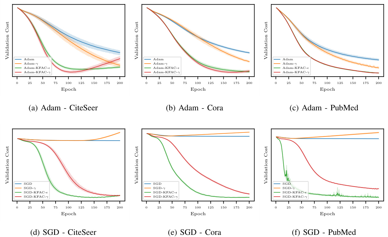
Fig. 1. The validation costs of four optimization methods on the second split of Citation datasets over 10 runs. A 2-layer GCN with a 64-dimensional hidden variable is used in all experiments. As shown in Fig. 1a, 1b, and 1c (upper row), the proposed Adam-KDAC methods (green and red curves) outperform vanilla Adam methods (blue and orange curves) on all three datasets. Also, Fig. 1d, 1e, and 1f (bottom row) reveal that the suggested SGD-KFAC methods (green and red curves) achieve a remarkably faster convergence than the vanilla SGD method (blue and orange curves) on all three datasets.
图 1: 四种优化方法在Citation数据集第二划分上10次运行的验证成本。所有实验均使用具有64维隐藏变量的2层GCN。如图1a、1b和1c(上行)所示,提出的Adam-KDAC方法(绿色和红色曲线)在所有三个数据集上均优于原始Adam方法(蓝色和橙色曲线)。此外,图1d、1e和1f(下行)表明,建议的SGD-KFAC方法(绿色和红色曲线)在所有三个数据集上比原始SGD方法(蓝色和橙色曲线)实现了显著更快的收敛。
As the original NGD (Eq. 14) is defined based on a prediction function with access only to a single sample, $p(\mathbf{y}|\mathbf{f}(\mathbf{x};\pmb\theta))$ , Fisher information matrix with the presence of the adjacency distribution becomes:
由于原始NGD (公式14) 是基于仅能访问单个样本的预测函数 $p(\mathbf{y}|\mathbf{f}(\mathbf{x};\pmb\theta))$ 定义的,存在邻接分布时的Fisher信息矩阵变为:
$$
\begin{array}{r l}&{F(\pmb\theta)=E_{\mathbf x,\underline{x}^{\prime},\underline{a},\mathbf y\sim p(\mathbf x,\underline{x}^{\prime},\underline{a},\mathbf y;\pmb\theta)}[\nabla_{\b\theta}\nabla_{\b\theta}^{\top}]}\ &{\qquad=E_{\mathbf x,\underline{x}^{\prime}\sim q(\mathbf x),\underline{a}\sim q({\boldsymbol a}|\mathbf x,\mathbf x^{\prime}),\mathbf y\sim p(\mathbf y|\mathbf x,\underline{x}^{\prime},\underline{a};\pmb\theta)}[\nabla_{\b\theta}\nabla_{\b\theta}^{\top}].}\end{array}
$$
$$
\begin{array}{r l}&{F(\pmb\theta)=E_{\mathbf x,\underline{x}^{\prime},\underline{a},\mathbf y\sim p(\mathbf x,\underline{x}^{\prime},\underline{a},\mathbf y;\pmb\theta)}[\nabla_{\b\theta}\nabla_{\b\theta}^{\top}]}\ &{\qquad=E_{\mathbf x,\underline{x}^{\prime}\sim q(\mathbf x),\underline{a}\sim q({\boldsymbol a}|\mathbf x,\mathbf x^{\prime}),\mathbf y\sim p(\mathbf y|\mathbf x,\underline{x}^{\prime},\underline{a};\pmb\theta)}[\nabla_{\b\theta}\nabla_{\b\theta}^{\top}].}\end{array}
$$
With $n$ samples of $q(\mathbf{x})$ , i.e. $X$ and $n^{2}$ samples of $q(a|X)$ , i.e. $A$ , Fisher can be estimated as:
在获得 $q(\mathbf{x})$ 的 $n$ 个样本 $X$ 以及 $q(a|X)$ 的 $n^{2}$ 个样本 $A$ 后,Fisher 信息量可估计为:
$$
\begin{array}{r}{\hat{F}(\pmb{\theta})=E_{\mathbf{y}\sim p(\mathbf{y}|X,A;\pmb{\theta})}[\nabla_{\pmb{\theta}}\nabla_{\pmb{\theta}}^{\mathsf{T}}],}\end{array}
$$
$$
\begin{array}{r}{\hat{F}(\pmb{\theta})=E_{\mathbf{y}\sim p(\mathbf{y}|X,A;\pmb{\theta})}[\nabla_{\pmb{\theta}}\nabla_{\pmb{\theta}}^{\mathsf{T}}],}\end{array}
$$
where
其中
$$
\nabla_{\pmb{\theta}}=-\nabla_{\pmb{\theta}}\log p(X,A,\mathbf{y};\pmb{\theta}).
$$
$$
\nabla_{\pmb{\theta}}=-\nabla_{\pmb{\theta}}\log p(X,A,\mathbf{y};\pmb{\theta}).
$$
In fact, to evaluate the expectation in Eq. 26, $q(X)$ and $q(A|X)$ are approximated with $\hat{q}(X)$ and $\hat{q}(A|X)$ using ${{\bf x}{i}}{i=1}^{n}$ and $A$ , respectively. However, there are only $\bar{n}$ samples from $\hat{q}(\mathbf{y}|\mathbf{x}{j})$ as an approximation of $q(\mathbf{y}|\mathbf{x}_{j})$ for the following replacement:
事实上,为了计算式26中的期望值,$q(X)$和$q(A|X)$分别通过${{\bf x}{i}}{i=1}^{n}$和$A$近似为$\hat{q}(X)$与$\hat{q}(A|X)$。但对于后续替换所需的$q(\mathbf{y}|\mathbf{x}{j})$,其近似分布$\hat{q}(\mathbf{y}|\mathbf{x}_{j})$仅能提供$\bar{n}$个样本。
$$
p(\mathbf{y}|X,A;\pmb{\theta})\approx\hat{q}(\mathbf{y}|\mathbf{x}_{i}).
$$
$$
p(\mathbf{y}|X,A;\pmb{\theta})\approx\hat{q}(\mathbf{y}|\mathbf{x}_{i}).
$$
Therefore, an empirical Fisher can be obtained by
因此,可以通过经验获得Fisher信息矩阵
for
为了
$$
\hat{F}(\pmb\theta)=\frac{1}{\bar{n}}\sum_{i=1}^{\bar{n}}\nabla_{\pmb\theta,i}\nabla_{\pmb\theta,i}^{\mathsf{T}}=\sum_{i=1}^{\bar{n}}B_{i}(\pmb\theta)
$$
$$
\hat{F}(\pmb\theta)=\frac{1}{\bar{n}}\sum_{i=1}^{\bar{n}}\nabla_{\pmb\theta,i}\nabla_{\pmb\theta,i}^{\mathsf{T}}=\sum_{i=1}^{\bar{n}}B_{i}(\pmb\theta)
$$
From the computation perspective, the matrix $B_{i}(\pmb\theta)$ can be very large, for example, in neural networks with multiple layers, the parameters could be huge, so it needs to be approximated too. In networks characterized with Eqs. 17 or 20, a simple solution would be ignoring the cross-layer terms so that $B_{i}(\pmb\theta)^{-1}$ and consequently $B_{i}(\pmb\theta)$ turns into a block-diagonal matrix:
从计算角度来看,矩阵$B_{i}(\pmb\theta)$可能非常大,例如在多层神经网络中参数量会极其庞大,因此也需要进行近似处理。对于式17或20描述的网络结构,一种简单解决方案是忽略跨层项,使$B_{i}(\pmb\theta)^{-1}$及对应的$B_{i}(\pmb\theta)$转化为块对角矩阵:
$$
B_{i}(\pmb\theta)=\mathrm{diag}(B_{1,i},\dots,B_{m,i})
$$
$$
B_{i}(\pmb\theta)=\mathrm{diag}(B_{1,i},\dots,B_{m,i})
$$
In KFAC, the diagonal block $B_{k,i}$ , corresponded to $k$ ’th layer with the dimension $d_{k}d_{k-1}\times d_{k}d_{k-1}$ , is approximated with the Kronecker product of the inverse of two smaller matrices $U_{k,i}$ and $V_{k,i}$ as:
在KFAC中,对应于第$k$层的对角块$B_{k,i}$(维度为$d_{k}d_{k-1}\times d_{k}d_{k-1}$)通过两个较小矩阵$U_{k,i}$和$V_{k,i}$的逆的Kronecker积来近似表示:
$$
B_{k,i}=(U_{k,i}\otimes V_{k,i})^{-1}=U_{k,i}^{-1}\otimes V_{k,i}^{-1}.
$$
$$
B_{k,i}=(U_{k,i}\otimes V_{k,i})^{-1}=U_{k,i}^{-1}\otimes V_{k,i}^{-1}.
$$
$U_{k}$ and $V_{k}$ blocks are approximated with the expected values of $\mathbf{u}{k,i}\mathbf{u}{k,i}^{\mathsf{T}}$ and $\mathbf{v}{k,i}\mathbf{v}{k,i}^{\mathsf{T}}$ respectively where $\mathrm{dim}({\mathbf{u}}{k})={d}{k}$ , $\dim(\mathbf{v}{k})=d_{k-1}$ . Finally, $U_{k}^{-1}$ and ${\cal V}{k}^{-1}$ are evaluated by taking inverses of $U_{k}+\epsilon^{-1/2}$ and $V_{k}+\epsilon^{-1/2}$ for $\epsilon$ being the regular iz ation hyper-parameter.
$U_{k}$ 和 $V_{k}$ 块分别用 $\mathbf{u}{k,i}\mathbf{u}{k,i}^{\mathsf{T}}$ 和 $\mathbf{v}{k,i}\mathbf{v}{k,i}^{\mathsf{T}}$ 的期望值近似,其中 $\mathrm{dim}({\mathbf{u}}{k})={d}{k}$,$\dim(\mathbf{v}{k})=d_{k-1}$。最后,通过求 $U_{k}+\epsilon^{-1/2}$ 和 $V_{k}+\epsilon^{-1/2}$ 的逆来计算 $U_{k}^{-1}$ 和 ${\cal V}_{k}^{-1}$,其中 $\epsilon$ 是正则化超参数。
For a graph with $n$ nodes, adjacency matrix $A$ , and the training set ${(\mathbf{x}{i},\mathbf{y}{i})}{i=1}^{\bar{n}}+{\mathbf{x}{i}}{i=\bar{n}+1}^{n}.$ , $U_{k}$ and $V_{k}$ are estimated in two ways: (1) using only $\bar{n}$ labeled samples, and (2) including $n-\bar{n}$ unlabeled samples. In the first method, $U_{k}$ and $V_{k}$ are estimated by:
对于一个具有 $n$ 个节点、邻接矩阵 $A$ 以及训练集 ${(\mathbf{x}{i},\mathbf{y}{i})}{i=1}^{\bar{n}}+{\mathbf{x}{i}}{i=\bar{n}+1}^{n}.$ 的图,$U_{k}$ 和 $V_{k}$ 通过两种方式估算:(1) 仅使用 $\bar{n}$ 个标注样本,(2) 包含 $n-\bar{n}$ 个未标注样本。在第一种方法中,$U_{k}$ 和 $V_{k}$ 通过以下方式估算:
$$
\begin{array}{c}{{U_{k}=\displaystyle{\frac{1}{\bar{n}}}\left({\frac{\partial l}{\partial X_{k}}}\odot\phi_{k}^{\prime}(W_{k}\tilde{X}{k-1})\right)\left({\frac{\partial l}{\partial X_{k}}}\odot\phi_{k}^{\prime}(W_{k}\tilde{X}{k-1})\right)^{\top}}}\ {{V_{k}=\displaystyle{\frac{1}{\bar{n}}}\tilde{X}{k-1}\tilde{X}_{k-1}^{\top}.}}\end{array}
$$
Note that both $\partial l/\partial X_{k}$ and $\phi_{k}^{\prime}(W_{k}\tilde{X}{k-1})$ are $d_{k}\times n$ matrices and the last $n-\bar{n}$ columns of $\partial l/\partial X_{k}$ are zero. However, as unlabeled samples are not used in the first method, one needs to evaluate loss function for $i={\bar{n}}+1,\dots,n$ , which can be done by sampling $\hat{\mathbf{y}}_{i}$ from $p(\mathbf{y}|\mathbf{x};\pmb\theta)$ . In the second method, these new samples are added to the empirical cost as
注意,$\partial l/\partial X_{k}$ 和 $\phi_{k}^{\prime}(W_{k}\tilde{X}{k-1})$ 都是 $d_{k}\times n$ 矩阵,且 $\partial l/\partial X_{k}$ 的最后 $n-\bar{n}$ 列为零。然而,由于第一种方法未使用未标记样本,需要为 $i={\bar{n}}+1,\dots,n$ 评估损失函数,这可以通过从 $p(\mathbf{y}|\mathbf{x};\pmb\theta)$ 中采样 $\hat{\mathbf{y}}_{i}$ 来实现。在第二种方法中,这些新样本被添加到经验成本中
$$
\begin{array}{l}{{\displaystyle{\hat{r}}(\pmb\theta)=\frac{1}{\bar{n}}\sum_{i=1}^{\bar{n}}l(\mathbf y_{i},f(X,A;\pmb\theta))}~}\ {{\displaystyle~+\frac{\lambda}{n-\bar{n}}\sum_{i=\bar{n}+1}^{n}l(\mathbf y_{i},f(X,A;\pmb\theta))},}\end{array}
$$
$$
\begin{array}{l}{{\displaystyle{\hat{r}}(\pmb\theta)=\frac{1}{\bar{n}}\sum_{i=1}^{\bar{n}}l(\mathbf y_{i},f(X,A;\pmb\theta))}~}\ {{\displaystyle~+\frac{\lambda}{n-\bar{n}}\sum_{i=\bar{n}+1}^{n}l(\mathbf y_{i},f(X,A;\pmb\theta))},}\end{array}
$$
where $0\leq\lambda\leq1$ denotes the regular iz ation hyper-parameter for controlling the cost of predicted labels and $\lambda=0$ results the first method. As the prediction improves over the course of training, $\lambda$ can be a function of iteration $t$ , for example here, it is defined to be:
其中 $0\leq\lambda\leq1$ 表示用于控制预测标签成本的正则化超参数,$\lambda=0$ 对应第一种方法。随着训练过程中预测效果的提升,$\lambda$ 可以是迭代次数 $t$ 的函数,例如在此定义为:
$$
\lambda(t):=\left(\frac{t}{\operatorname*{max}(t)}\right)^{\gamma},
$$
$$
\lambda(t):=\left(\frac{t}{\operatorname*{max}(t)}\right)^{\gamma},
$$
where $\operatorname*{max}(t)$ shows the maximum number of iterations and $\gamma$ is the replaced regular iz ation hyper-parameter. Algorithm 1 shows the preconditioning step for modifying gradients of each layer at any iteration such that gradients are first, transformed using two matrices of ${\cal V}{k}^{-1}$ and $U_{k}^{-1}$ , then sent to the optimization algorithm for updating parameters.
其中 $\operatorname*{max}(t)$ 表示最大迭代次数,$\gamma$ 为替换的正则化超参数。算法1展示了在每次迭代中修改各层梯度的预处理步骤:梯度首先通过 ${\cal V}{k}^{-1}$ 和 $U_{k}^{-1}$ 两个矩阵进行变换,随后传递至优化算法以更新参数。
A. Relation between Fisher and Hessian
A. Fisher与Hessian矩阵的关系
The Hessian of the cost function:
代价函数的 Hessian 矩阵:
$$
H_{\pmb\theta}r(\pmb\theta)=E_{X,A,\mathbf y\sim p(X,A,\mathbf y;\pmb\theta)}[H_{\pmb\theta}l(\mathbf y,f(X,A;\pmb\theta))]
$$
$$
H_{\pmb\theta}r(\pmb\theta)=E_{X,A,\mathbf y\sim p(X,A,\mathbf y;\pmb\theta)}[H_{\pmb\theta}l(\mathbf y,f(X,A;\pmb\theta))]
$$
Algorithm 1 Semi-Supervised Preconditioning
算法 1 半监督预处理
| Require: VWk | 参数梯度 (k = 1, ..., m) |
| Require: A | 邻接矩阵 |
| Require: D | 度矩阵 |
| Require: Z | 训练掩码向量 |
| Require: ∈, λ | 正则化超参数 |
$$
\begin{array}{r l}{n=\dim(\mathbf{z})} {\bar{n}=\sum(\mathbf{z})}{\tilde{A}=(D+I)^{-1/2}(A+I)(D+I)^{-1/2}=[\tilde{a}_{i j}]}\end{array}
$$
$$
\begin{array}{r l}&{n=\dim(\mathbf{z})}\ &{\bar{n}=\sum(\mathbf{z})}\ &{\tilde{A}=(D+I)^{-1/2}(A+I)(D+I)^{-1/2}=[\tilde{a}_{i j}]}\end{array}
$$
for $k=1,\ldots,m$ do
对于 $k=1,\ldots,m$ 执行
$$
\begin{array}{r l}&{\tilde{\mathbf{x}}{k-1,i}=\sum_{j=1}^{n}\tilde{a}{i,j}\mathbf{x}{k-1,j}}\ &{\mathbf{u}{k-1,i}=\partial l/\partial\mathbf{x}{k}\odot\boldsymbol{\phi}{k}^{\prime}(W_{k}\tilde{\mathbf{x}}{k-1,i})}\ &{\mathbf{v}{k-1,i}=\tilde{\mathbf{x}}{k-1,i}}\ &{U_{k}=\sum_{i=1}^{n}(z_{i}+(1-z_{i})\lambda)\mathbf{u}{k-1,i}\mathbf{u}{k-1,i}^{\mathsf{T}}/(n+\lambda\bar{n})}\ &{V_{k}=\sum_{i=1}^{n}(z_{i}+(1-z_{i})\lambda)\mathbf{v}{k,i}\mathbf{v}{k,i}^{\mathsf{T}}/(n+\lambda\bar{n})}\ &{U_{k}^{-1}=\mathrm{INVERSE}(U_{k})}\ &{V_{k}^{-1}=\mathrm{INVERSE}(V_{k})}\end{array}
$$
function INVERSE $(X)$ output $(X+\epsilon^{-1/2}I)^{-1}$
函数 INVERSE $(X)$ 输出 $(X+\epsilon^{-1/2}I)^{-1}$
can also be approximated using ${\hat{q}}(X),{\hat{q}}(A|X)$ , and ${\hat{q}}(\mathbf{y}|\mathbf{x}_{i})$ resulting the empirical Hessian to be
也可通过 ${\hat{q}}(X)$、${\hat{q}}(A|X)$ 和 ${\hat{q}}(\mathbf{y}|\mathbf{x}_{i})$ 进行近似,从而得到经验Hessian矩阵
$$
\hat{H}{\pmb\theta}r(\pmb\theta):=\frac{1}{\bar{n}}\sum_{i=1}^{\bar{n}}H_{\pmb\theta}l(\mathbf y_{i},f(X,A;\pmb\theta)),
$$
$$
\hat{H}{\pmb\theta}r(\pmb\theta):=\frac{1}{\bar{n}}\sum_{i=1}^{\bar{n}}H_{\pmb\theta}l(\mathbf y_{i},f(X,A;\pmb\theta)),
$$
which is equivalent to the empirical Fisher Eq. 31 when $p(X,A,\mathbf{y};\pmb\theta)$ is estimated with $\hat{q}(X)\hat{q}(A|X)\hat{q}(\mathbf{y}|\mathbf{x}_{i})$ for $i=1,\ldots,\bar{n}$ (see Lemma 1 in the appendix).
这等价于当用$\hat{q}(X)\hat{q}(A|X)\hat{q}(\mathbf{y}|\mathbf{x}_{i})$对$i=1,\ldots,\bar{n}$估计$p(X,A,\mathbf{y};\pmb\theta)$时的经验Fisher方程(见附录中的引理1)。
IV. EXPERIMENTS
IV. 实验
In this section, the performance of the proposed algorithm is evaluated compared to Adam and SGD on several datasets for the task of node classification in single graphs. The task is assumed to be trans duct ive when all the features are available for training but only a portion of labels are used in the training. First, a detailed description of datasets and the model architecture are provided. Then, the general optimization setup, commonly used for the node classification, is specified. The last part includes the sensitivity to hyper-parameter and training time analysis in addition to validation cost convergence and the test accuracy. All the experiments are conducted mainly using Pytorch [19] and Pytorch Geometric [5], two open-source Python libraries for automating differentiation and working with graph datasets.
在本节中,我们将所提算法与Adam和SGD在多个数据集上针对单图节点分类任务的性能进行比较。该任务被设定为直推式学习 (transductive learning) ,即训练时所有节点特征可用但仅部分标签参与训练。首先详细描述数据集与模型架构,随后说明节点分类任务通用的优化配置。最后部分除验证损失收敛性和测试精度外,还包含超参数敏感性分析及训练时长评估。所有实验主要基于两个开源Python库实现:自动化微分框架PyTorch [19] 和图数据处理库PyTorch Geometric [5]。
A. Datasets
A. 数据集
Three citation datasets with the statistics shown in Table II are used in the experiments [21]. Cora, CiteSeer, and PubMed are single graphs in which nodes and edges correspond to documents and citation links, respectively. A sparse feature vector (document keywords) and a class label are associated with each node. Several splits of these datasets are used in the node classification task. The first split, 20 instances are randomly selected for training, 500 for validation, and 1000 for the test; the rest of the labels are not used [23]. In the second split, all nodes except $500{+}1000$ validation and test nodes are used for the training [3]. To evaluate the over fitting behavior, the third split exploits all labels for training excluding $500+500$ nodes for the validation and test [15].
实验中使用了三个引用数据集,其统计信息如表 II 所示[21]。Cora、CiteSeer 和 PubMed 是单图结构,其中节点和边分别对应文档和引用链接。每个节点关联一个稀疏特征向量(文档关键词)和一个类别标签。在节点分类任务中采用了这些数据集的多种划分方式:
- 第一种划分:随机选择 20 个实例用于训练,500 个用于验证,1000 个用于测试,其余标签不作使用[23];
- 第二种划分:除 $500{+}1000$ 个验证和测试节点外,所有节点均用于训练[3];
- 第三种划分:为评估过拟合行为,使用除 $500+500$ 个验证和测试节点外的全部标签进行训练[15]。
TABLE II CITATION NETWORK DATASETS STATISTICS
表 II 引用网络数据集统计
| 数据集 | 节点数 | 边数 | 类别数 | 特征数 |
|---|---|---|---|---|
| Citeseer | 3,327 | 4,732 | 6 | 3,703 |
| Cora | 2,708 | 5,429 | 7 | 1,433 |
| Pubmed | 19,717 | 44,338 | 3 | 500 |
B. Architectures
B. 架构
In the node classification using a NN followed by Softmax function (Eq. 5), the class with maximum probability is chosen to be the predicted node label. A 2-layer GCN with a 64- dimensional hidden variable is used for comparing different optimization methods. In the first
在使用神经网络后接Softmax函数(公式5)进行节点分类时,选择概率最大的类别作为预测节点标签。为了比较不同优化方法,我们采用了一个具有64维隐藏变量的2层GCN。在第一个
layer, the activation function ReLU is followed by a dropout function with a rate of 0.5. The loss function is evaluated as the negative log-likelihood of Softmax (Eq. 5) of the last layer.
在每一层中,激活函数ReLU后接一个丢弃率为0.5的dropout函数。损失函数通过最后一层Softmax (公式5) 的负对数似然进行评估。
C. Optimization
C. 优化
The weights of parameters are initialized like the original GCN [10] and input vectors are row-normalized accordingly [7]. The model is trained for 200 epochs without any early stopping and the learning rate of 0.01. The Adam and SGD are used with the weight decay of $5\times10^{-4}$ and the momentum of 0.9, respectively.
参数权重初始化方式与原始GCN [10]相同,输入向量按[7]所述进行行归一化。模型训练200个epoch且不采用早停策略,学习率为0.01。分别使用Adam和SGD优化器,权重衰减为$5\times10^{-4}$,动量设置为0.9。
D. Results
D. 结果
The optimization performance is measured by both the minimum validation cost and the test accuracy for the best validation cost. The validation cost of training a 2-layer GCN with a 64-dimensional hidden variable is used for comparing optimization methods (Adam and SGD) with their preconditioned version (Adam-KFAC and SGD-KFAC). For each method, unlabeled samples are used in the training process with a ratio controlled by $\gamma$ . Fig. 1 shows the validation cost of four methods based on Adam (upper row) and SGD (bottom row) for all three Citation datasets. The test accuracy of a 2-layer GCN trained using four different methods on three split are shown in Tab. III, IV, and V. Reported values of test accuracy in tables are averages and $95%$ confidence intervals over 10 runs for the best hyper-parameters tuned on the second split of the CiteSeer dataset. Note that the test accuracy may not always reflect the performance of the optimization method as the objective function (cross-entropy) is not the same as the prediction function (argmax). However, in most cases, the proposed method achieves better accuracy compared to Adam (the first row in all tables). As a fixed learning rate 0.01 is used in all methods, SGD has a very slow convergence and does not provide competitive results.
优化性能通过最佳验证成本下的最小验证成本和测试准确率来衡量。使用具有64维隐藏变量的2层GCN (Graph Convolutional Network) 训练验证成本来比较优化方法 (Adam和SGD) 及其预条件版本 (Adam-KFAC和SGD-KFAC)。每种方法的训练过程中使用未标记样本,其比例由 $\gamma$ 控制。图1展示了基于Adam (上排) 和SGD (下排) 的四种方法在所有三个Citation数据集上的验证成本。表III、IV和V分别展示了使用四种不同方法训练的2层GCN在三种数据划分下的测试准确率。表中报告的测试准确率值为在CiteSeer数据集第二种划分上调优最佳超参数后10次运行的平均值及 $95%$ 置信区间。需要注意的是,由于目标函数 (交叉熵) 与预测函数 (argmax) 不同,测试准确率并不总能反映优化方法的性能。然而在大多数情况下,所提方法相比Adam (所有表格中的第一行) 获得了更高的准确率。由于所有方法均采用固定学习率0.01,SGD收敛速度极慢且未能提供有竞争力的结果。
The importance of hyper-parameters $\epsilon$ , $\gamma$ are shown in Fig. 2. Figures 2a and 2d depict the sensitivity of Adam and SGD to the $\epsilon$ parameter, respectively. As the inverse of $\epsilon$ directly affects the same factor as the learning rate $\eta$ , the smaller the $\epsilon$ , the faster the convergence. However, choosing very small $\epsilon$ results in larger confidence intervals which are not desirable. The effect of $\gamma$ on Adam and SGD are depicted in figures 2b and 2e, respectively. When using Adam, due to its faster convergence compared to SGD, smaller $\gamma$ , i.e. using more predictions leads to much wider confidence intervals. In other words, the training process dominated by more labels results in a more stable convergence with a smaller variance. Thus, for a stable estimation, $\lambda$ or $\gamma$ must be tuned with respect to the optimization algorithm because of their sensitivity to the convergence rate. Since the Fisher matrix does not change considerably at each iteration, an experiment is performed to explore the sensitivity of validation loss to the frequency of updating Fisher. In Figures 2c and 2f, the validation cost over time is evaluated for updating Fisher every $4,8,\ldots,128$ iterations. When Fisher is updated more frequently, its computation takes more time hence the training process lasts longer (having other hyper-parameters fixed). Increasing the update frequency does not affect the performance to some extent, however, it largely reduces the training time. As updating Fisher every 50 or 100 iterations, does not affect the final validation cost to a great extent, to speed up the training process, Fisher is updated every 50 epochs in all of the experiments.
超参数 $\epsilon$ 和 $\gamma$ 的重要性如图 2 所示。图 2a 和图 2d 分别展示了 Adam 和 SGD 对 $\epsilon$ 参数的敏感性。由于 $\epsilon$ 的倒数与学习率 $\eta$ 直接影响相同因子,$\epsilon$ 越小,收敛速度越快。然而,选择过小的 $\epsilon$ 会导致置信区间变大,这是不理想的。$\gamma$ 对 Adam 和 SGD 的影响分别在图 2b 和图 2e 中展示。使用 Adam 时,由于其收敛速度比 SGD 快,较小的 $\gamma$(即使用更多预测)会导致置信区间显著变宽。换句话说,由更多标签主导的训练过程会带来更稳定的收敛和更小的方差。因此,为了稳定估计,必须根据优化算法调整 $\lambda$ 或 $\gamma$,因为它们对收敛速度非常敏感。
由于 Fisher 矩阵在每次迭代中变化不大,我们通过实验验证了验证损失对 Fisher 更新频率的敏感性。在图 2c 和图 2f 中,评估了每 $4,8,\ldots,128$ 次迭代更新 Fisher 时的验证成本随时间的变化。Fisher 更新越频繁,计算耗时越长,训练过程也相应延长(其他超参数固定时)。增加更新频率在一定程度上不影响性能,但会大幅减少训练时间。由于每 50 或 100 次迭代更新 Fisher 对最终验证成本影响较小,为了加速训练过程,所有实验中 Fisher 均每 50 轮更新一次。
TABLE III THE TEST ACCURACY OF FOUR OPTIMIZATION METHODS ON THE FIRST SPLIT OF CITATION DATASETS OVER 10 RUNS. A 2-LAYER GCN WITH A 64-DIMENSIONAL HIDDEN VARIABLE IS USED IN ALL EXPERIMENTS.
表 III 四种优化方法在CITATION数据集第一个划分上10次运行的测试准确率。所有实验均使用具有64维隐藏变量的2层GCN。
| CiteSeer | Cora | Pubmed | |
|---|---|---|---|
| Adam | 71.66 ± 0.61 | 81.20 ± 0.25 | 79.72 ± 0.30 |
| Adam | 74.28 ± 0.67 | 82.42 ± 0.33 | 80.06 ± 0.34 |
| Adam-KFAC | 71.94 ± 0.53 | 81.68 ± 0.25 | 79.48 ± 0.28 |
| Adam-KFAC | 70.24 ± 0.66 | 82.84 ± 0.87 | 76.94 ± 0.59 |
| SGD | 20.38 ± 8.92 | 23.14 ± 5.17 | 45.76 ± 3.04 |
| SGDr | 17.64 ± 6.18 | 17.26 ± 8.41 | 46.20 ± 4.35 |
| SGD-KFACe | 71.82 ± 0.48 | 82.06 ± 0.34 | 77.20 ± 0.63 |
| SGD-KFAC- | 73.52 ± 0.22 | 81.70 ± 0.79 | 79.20 ± 0.29 |
TABLE IV THE TEST ACCURACY OF FOUR OPTIMIZATION METHODS ON THE SECOND SPLIT OF CITATION DATASETS OVER 10 RUNS. A 2-LAYER GCN WITH A 64-DIMENSIONAL HIDDEN VARIABLE IS USED IN ALL EXPERIMENTS.
表 IV 四种优化方法在CITATION数据集第二划分上10次运行的平均测试准确率。所有实验均使用具有64维隐藏变量的2层GCN。
| CiteSeer | Cora | Pubmed | |
|---|---|---|---|
| Adam | 78.68 ± 0.83 | 87.36 ± 0.47 | 87.78 ± 0.14 |
| Adam | 77.98 ± 0.39 | 87.28 ± 0.34 | 87.52 ± 0.30 |
| Adam-KFAC | 79.50 ± 0.15 | 87.60 ± 0.20 | 88.46 ± 0.24 |
| Adam-KFAC | 79.42 ± 0.32 | 86.60 ± 0.30 | 87.88 ± 0.16 |
| SGD | 20.80 ± 2.12 | 31.90 ± 0.00 | 43.22 ± 1.42 |
| SGD | 20.96 ± 5.22 | 31.90 ± 0.00 | 40.82 ± 0.33 |
| SGD-KFACe | 79.48 ± 0.40 | 87.54 ± 0.43 | 89.08 ± 0.18 |
| SGD-KFAC | 77.32 ± 0.27 | 87.42 ± 0.24 | 88.18 ± 0.30 |
TABLE V THE TEST ACCURACY OF FOUR OPTIMIZATION METHODS ON THE THIRD SPLIT OF CITATION DATASETS OVER 10 RUNS. A 2-LAYER GCN WITH A 64-DIMENSIONAL HIDDEN VARIABLE IS USED IN ALL EXPERIMENTS.
表 V 四种优化方法在引用数据集第三次划分上经过10次运行的测试准确率。所有实验均使用具有64维隐藏变量的2层GCN。
| CiteSeer | Cora | Pubmed | |
|---|---|---|---|
| Adam | 79.80 ± 0.66 | 89.44 ± 0.41 | 87.16 ± 0.71 |
| Adam | 79.64 ± 0.32 | 89.60 ± 0.91 | 87.44 ± 0.27 |
| Adam-KFAC | 80.52 ± 0.14 | 90.16 ± 0.59 | 87.84 ± 0.21 |
| Adam-KFAC | 80.52 ± 0.22 | 89.24 ± 0.64 | 87.36 ± 0.37 |
| SGD | 15.04 ± 1.70 | 32.80 ± 0.00 | 41.96 ± 0.44 |
| SGDr | 16.12 ± 5.30 | 32.80 ± 0.00 | 41.20 ± 0.00 |
| SGD-KFACe | 79.76 ± 0.75 | 89.88 ± 0.14 | 89.36 ± 0.57 |
| SGD-KFAC | 78.52 ± 0.28 | 88.72 ± 0.38 | 87.88 ± 0.80 |

Fig. 2. The sensitivity of $\epsilon,\gamma$ , and updating frequency on validation costs of Adam-KFAC (upper) and SGD-KFAC (below) when training on the second split of CiteSeer dataset over 10 runs. A 2-layer GCN with a 64-dimensional hidden variable is used in all experiments. Fig. 2a and 2d show that smaller $\epsilon$ results in a faster convergence with a probable cost of larger variance as it inversely scales the same factor as the learning rate. As depicted in Fig. 2b and 2e, the larger the $\gamma$ , the more stable the convergence (the more confined confidence intervals). Finally, it can be seen in Fig. 2c and 2f that since performances are similar under different updating frequencies, selecting a relatively large frequency (50) can reduce the training time substantially.
图 2: 在CiteSeer数据集第二划分上训练10次时,Adam-KFAC(上)和SGD-KFAC(下)对$\epsilon,\gamma$及更新频率的验证成本敏感性。所有实验均使用具有64维隐藏变量的2层GCN。图2a和2d显示,较小的$\epsilon$会带来更快的收敛速度,但可能以更大方差为代价,因为它与学习率成反比缩放。如图2b和2e所示,$\gamma$越大,收敛越稳定(置信区间越窄)。最后从图2c和2f可见,由于不同更新频率下性能相似,选择较大频率(50)可大幅减少训练时间。
To examine the time complexity of the proposed method, the validation costs of AdamKFAC and SGD-KFAC are compared with Adam and SGD when training on the second split of Citation datasets with respect to the training time for 200 epochs (Fig. 3). The training on
为了检验所提方法的时间复杂度,在Citation数据集的第二个分割上训练200个周期时,将AdamKFAC和SGD-KFAC的验证成本与Adam和SGD进行了对比(图3)。训练过程中
Cora and PubMed (Fig. 3b and 3c) takes a shorter time compared to the training on CitSeer (Fig. 3a) mainly because of the dimension of input features as it directly enlarges the size of the Fisher matrix. As shown in Fig. 3, the proposed SGD-KFAC method (red curve) converges much faster than the vanilla SGD as expected. Surprisingly, SGD-KFAC outperforms Adam and even Adam-KFAC methods in all datasets implying that the naive SGD with a natural gradient pre conditioner can lead to a faster convergence than Adam-based methods. Another interesting observation is that Adam-based methods demonstrate similar performances in all experiments making them independent of the dataset while SGD-based methods show different over fitting behavior.
与在CitSeer (图3a) 上的训练相比,Cora和PubMed (图3b和3c) 耗时更短,主要原因是输入特征的维度会直接扩大Fisher矩阵的规模。如图3所示,所提出的SGD-KFAC方法 (红色曲线) 如预期般比普通SGD收敛快得多。令人惊讶的是,SGD-KFAC在所有数据集上都优于Adam甚至Adam-KFAC方法,这表明带有自然梯度预调节器的朴素SGD能比基于Adam的方法实现更快的收敛。另一个有趣的观察是,基于Adam的方法在所有实验中表现相似,使其不受数据集影响,而基于SGD的方法则展现出不同的过拟合行为。

Fig. 3. The validation costs of four optimization methods with respect to the training time on the second split of Citation datasets over 10 runs. A 2-layer GCN with a 64-dimensional hidden variable is used in all experiments. The proposed SGD-KFAC method shows the highest convergence rate among all other methods and it is slightly faster than Adam-KFAC.
图 3: 四种优化方法在Citation数据集第二个划分上的10次运行验证成本随训练时间变化曲线。所有实验均使用含64维隐变量的2层GCN。提出的SGD-KFAC方法在所有方法中收敛速度最快,略优于Adam-KFAC。
V. CONCLUSION
V. 结论
In this work, we introduced a novel optimization framework for graph-based semi-supervised learning. After the distinct definition of semi-supervised problems with the adjacency distribution, we provided a comprehensive review of topics like semi-supervised learning, graph neural network, and preconditioning optimization (and NGD as its especial case). We adopted a commonly used probabilistic framework covering least-squared regression and cross-entropy classification. In the node classification task, our proposed method showed to improve Adam and SGD not only in the validation cost but also in the test accuracy of GCN on three splits of Citation datasets. Extensive experiments were provided on the sensitivity to hyper-parameters and the time complexity. As the first work, to the best of our knowledge, on the preconditioned optimization of graph neural networks, we not only achieved the best test accuracy but also empirically showed that it can be used with both Adam and SGD.
在本工作中,我们提出了一种新颖的基于图的半监督学习优化框架。在通过邻接分布明确定义半监督问题后,我们对半监督学习、图神经网络和预处理优化(以及其特例NGD)等主题进行了全面综述。我们采用了一个涵盖最小二乘回归和交叉熵分类的常用概率框架。在节点分类任务中,我们提出的方法在GCN对Citation数据集三种划分的验证成本和测试准确率上均优于Adam和SGD。我们还对超参数敏感性和时间复杂度进行了大量实验。据我们所知,这是首个关于图神经网络预处理优化的研究,我们不仅取得了最佳测试准确率,还通过实验证明该方法可同时适用于Adam和SGD。
As the pre conditioner may significantly affect Adam, illustrating the relation between NGD and Adam and effectively combining them can be a promising direction for future work. We also aim to deploy faster approximation methods than KFAC like [6] and better sampling methods for exploiting unlabeled samples. Finally, since this work is mainly focused on single parameter layers, another possible research path would be adjusting KFAC to, for example, residual layers [8].
由于预调节器可能显著影响Adam,阐明NGD与Adam之间的关系并有效结合二者或将成为未来工作的可行方向。我们同时致力于部署比KFAC更快的近似方法(如[6])以及更好的采样方法来利用未标注样本。最后,鉴于本研究主要聚焦单参数层,另一潜在研究方向可能是调整KFAC以适配残差层等结构[8]。