Acceptability Judgements via Examining the Topology of Attention Maps

通过注意力图拓扑分析可接受性判断

Abstract

摘要

The role of the attention mechanism in encoding linguistic knowledge has received special interest in NLP. However, the attention heads’ ability to judge the grammatical acceptability of a sentence has been under explored. This paper approaches the paradigm of acceptability judgments with topological data analysis (TDA), showing that the topological properties of the attention graph can be efficiently exploited for two standard practices in linguistics: binary judgments and linguistic minimal pairs. Topological features enhance the BERTbased acceptability classifier scores by up to 0.24 Matthew’s correlation coefficient score on COLA in three languages (English, Italian, and Swedish). By revealing the topological discrepancy between attention graphs of minimal pairs, we achieve the human-level performance on the BLIMP benchmark, outperforming nine statistical and Transformer LM baselines. At the same time, TDA provides the foundation for analyzing the linguistic functions of attention heads and interpreting the correspondence between the graph features and grammatical phenomena. We publicly release the code and other materials used in the experiments 1.

注意力机制在编码语言知识中的作用一直受到自然语言处理领域的特别关注。然而，注意力头对句子语法可接受性的判断能力尚未得到充分研究。本文采用拓扑数据分析 (TDA) 方法研究可接受性判断范式，证明注意力图的拓扑特性可有效应用于语言学中的两种标准实践：二元判断和语言学最小对立对。在英语、意大利语和瑞典语三种语言的COLA数据集上，拓扑特征将基于BERT的可接受性分类器的马修斯相关系数最高提升了0.24。通过揭示最小对立对注意力图的拓扑差异，我们在BLIMP基准测试中达到人类水平表现，优于九种统计模型和Transformer语言模型基线。同时，TDA为分析注意力头的语言功能、解释图特征与语法现象之间的对应关系提供了基础。我们公开了实验中使用的代码和其他材料[1]。

1 Introduction

1 引言

Linguistic competence of neural language models (LMs) has emerged as one of the core sub-fields in NLP. The research paradigms explore whether Transformer LMs (Vaswani et al., 2017) induce linguistic generalizations from raw pre-training corpora (Warstadt et al., 2020b; Zhang et al., 2021), what properties are learned during task-specific fine-tuning (Miaschi et al., 2020; Merchant et al., 2020), and how the experimental results are connected to grammar and language acquisition theories (Pater, 2019; Manning et al., 2020).

神经语言模型的语言能力已成为自然语言处理(NLP)的核心子领域之一。该研究范式主要探索：Transformer模型(Vaswani等，2017)能否从原始预训练语料中归纳语言泛化规律(Warstadt等，2020b；Zhang等，2021)，在任务特定微调过程中学习了哪些特性(Miaschi等，2020；Merchant等，2020)，以及实验结果如何与语法和语言习得理论相关联(Pater，2019；Manning等，2020)。

One of these paradigms is centered around acce pt ability judgments, which have formed an empirical foundation in generative linguistics over the last six decades (Chomsky, 1965; Schütze, 1996; Scholz et al., 2021). Acceptability of linguistic stimuli is traditionally investigated in the form of a forced choice between binary categories or minimal pairs (Sprouse, 2018), which are widely adopted for acceptability classification (Linzen et al., 2016; Warstadt et al., 2019) and probabilistic LM scoring (Lau et al., 2017).

其中一种范式围绕可接受性判断展开，这些判断构成了生成语言学过去六十年的实证基础 (Chomsky, 1965; Schütze, 1996; Scholz et al., 2021)。传统上，语言刺激的可接受性通过二元类别或最小对立对的强制选择形式进行研究 (Sprouse, 2018)，这种方法被广泛用于可接受性分类 (Linzen et al., 2016; Warstadt et al., 2019) 和概率性大语言模型评分 (Lau et al., 2017)。

A scope of approaches has been proposed to interpret the roles of hundreds of attention heads in encoding linguistic properties (Htut et al., 2019; Wu et al., 2020) and identify how the most influential ones benefit the downstream performance (Voita et al., 2019; Jo and Myaeng, 2020). Prior work has demonstrated that heads induce grammar formalisms and structural knowledge (Zhou and Zhao, 2019; Lin et al., 2019; Luo, 2021), and linguistic features motivate attention patterns (Kovaleva et al., 2019; Clark et al., 2019). Recent studies also show that certain heads can have multiple functional roles (Pande et al., 2021) and even perform syntactic functions for typologically distant languages (Ravi shankar et al., 2021).

已有多种方法被提出，用于解释数百个注意力头(attention head)在编码语言属性中的作用 [Htut et al., 2019; Wu et al., 2020]，并识别最具影响力的头如何提升下游任务性能 [Voita et al., 2019; Jo and Myaeng, 2020]。先前研究表明，这些头能诱导语法形式体系和结构知识 [Zhou and Zhao, 2019; Lin et al., 2019; Luo, 2021]，而语言特征会驱动注意力模式 [Kovaleva et al., 2019; Clark et al., 2019]。最新研究还发现，某些头可能具有多重功能角色 [Pande et al., 2021]，甚至能为类型学差异较大的语言执行句法功能 [Ravi shankar et al., 2021]。

Our paper presents one of the first attempts to analyze attention heads in the context of linguistic acceptability (LA) using topological data analysis $(\mathrm{TDA}^{2}$ ; Chazal and Michel, 2017). TDA allows for exploiting complex structures underlying textual data and investigating graph representations of Transformer’s attention maps. We show that topological features are sensitive to well-established LA contrasts, and the grammatical phenomena can be encoded with the topological properties of the attention map.

我们的论文首次尝试在语言可接受性(LA)分析中运用拓扑数据分析(TDA)来研究注意力头机制。该方法能有效挖掘文本数据的复杂结构，并探究Transformer注意力图表的拓扑表征。研究表明，拓扑特征对经典LA对比敏感，且语法现象可通过注意力图的拓扑属性进行编码。

The main contributions are the following: (i) We adapt TDA methods to two standard approaches to LA judgments: acceptability classification and scoring minimal pairs (§3). (ii) We conduct acceptability classification experiments in three Indo-European languages (English, Italian, and Swedish) and outperform the established baselines (§4). (iii) We introduce two scoring functions, which reach the human-level performance in discr imina ting between minimal pairs in English and surpass nine statistical and Transformer LM baselines (§5). $(i\nu)$ The linguistic analysis of the feature space proves that TDA can serve as a complementary approach to interpreting the attention mechanism and identifying heads with linguistic functions $(\S4.3,\S5.3,\S6)$ .

主要贡献如下：(i) 我们将TDA方法适配至语言可接受性判断的两种标准方法：可接受性分类与最小对立对评分(第3节)。(ii) 在三种印欧语系语言(英语、意大利语和瑞典语)中开展可接受性分类实验，性能超越现有基线(第4节)。(iii) 提出两种评分函数，在英语最小对立对判别任务中达到人类水平表现，并超越九种统计方法与Transformer语言模型基线(第5节)。$(i\nu)$ 特征空间的语言学分析证明，TDA可作为解释注意力机制和识别具有语言学功能头部的补充方法(第4.3节、第5.3节、第6节)。

2 相关工作

2.1 Linguistic Acceptability

2.1 语言可接受性

Acceptability Classification. Early works approach acceptability classification with classic ML methods, hand-crafted feature templates, and probabilistic syntax parsers (Cherry and Quirk, 2008; Wagner et al., 2009; Post, 2011). Another line employs statistical LMs (Heilman et al., 2014), including threshold-based classification with LM scoring functions (Clark et al., 2013). The ability of RNN-based models (Elman, 1990; Hochreiter and Schmid huber, 1997) to capture long-distance regularities has stimulated investigation of their grammatical sensitivity (Linzen et al., 2016). With the release of the Corpus of Linguistic Acceptability (COLA; Warstadt et al., 2019) and advances in language modeling, the focus has shifted towards Transformer LMs (Yin et al., 2020), establishing LA as a proxy for natural language understanding (NLU) abilities (Wang et al., 2018) and linguistic competence of LMs (Warstadt and Bowman, 2019).

可接受性分类。早期研究采用经典机器学习方法、手工制作的特征模板和概率句法分析器处理可接受性分类 (Cherry and Quirk, 2008; Wagner et al., 2009; Post, 2011)。另一方向使用统计语言模型 (Heilman et al., 2014)，包括基于阈值的语言模型评分函数分类 (Clark et al., 2013)。基于RNN的模型 (Elman, 1990; Hochreiter and Schmidhuber, 1997) 捕捉长距离规律的能力激发了对它们语法敏感性的研究 (Linzen et al., 2016)。随着语言可接受性语料库 (COLA; Warstadt et al., 2019) 的发布和语言建模技术的进步，研究重点转向Transformer语言模型 (Yin et al., 2020)，将语言可接受性作为衡量自然语言理解能力 (Wang et al., 2018) 和语言模型语言能力 (Warstadt and Bowman, 2019) 的代理指标。

Linguistic Minimal Pairs. A forced choice between minimal pairs is a complementary approach to LA, which evaluates preferences between pairs of sentences that contrast an isolated grammatical phenomenon (Schütze, 1996). The idea of discriminating between minimal contrastive pairs has been widely applied to scoring generated hypotheses in downstream tasks (Pauls and Klein, 2012; Salazar et al., 2020), measuring social biases (Nangia et al., 2020), analyzing machine translation models (Burlot and Yvon, 2017; Sennrich, 2017), and linguistic profiling of LMs in multiple languages (Marvin and Linzen, 2018; Mueller et al., 2020).

语言最小对立对。在最小对立对之间进行强制选择是语言可接受性(LA)的一种补充方法，它评估在孤立语法现象上形成对比的句子对之间的偏好 (Schütze, 1996)。区分最小对比对的思想已广泛应用于下游任务中生成假设的评分 (Pauls and Klein, 2012; Salazar et al., 2020)、测量社会偏见 (Nangia et al., 2020)、分析机器翻译模型 (Burlot and Yvon, 2017; Sennrich, 2017) 以及多语言大语言模型的语言特征分析 (Marvin and Linzen, 2018; Mueller et al., 2020)。

2.2 Topological Data Analysis in NLP

2.2 NLP中的拓扑数据分析

TDA has found several applications in NLP. One of them is word sense induction by clustering word graphs and detecting their connected components. The graphs can be built from word dictionaries (Levary et al., 2012), association net- works (Dubuisson et al., 2013), and word vector representations (Jakubowski et al., 2020). Another direction involves building class if i ers upon geometric structural properties for movie genre detection (Doshi and Zadrozny, 2018), textual entail- ment (Savle et al., 2019), and document classification (Das et al., 2021; Werenski et al., 2022). Recent works have mainly focused on the topology of LMs’ internal representations. Kushnareva et al. (2021) represent attention maps with TDA features to approach artificial text detection. Colombo et al. (2021) introduce BARYSCORE, an automatic evaluation metric for text generation that relies on Wasser stein distance and barycenter s. To the best of our knowledge, TDA methods have not yet been applied to LA.

TDA在自然语言处理(NLP)领域已有多个应用方向。其一是通过聚类词图并检测连通分量来实现词义归纳，这些词图可基于词典(Levary et al., 2012)、关联网络(Dubuisson et al., 2013)或词向量表示(Jakubowski et al., 2020)构建。另一研究方向是利用几何结构特性构建分类器，应用于电影类型检测(Doshi and Zadrozny, 2018)、文本蕴含(Savle et al., 2019)及文档分类(Das et al., 2021; Werenski et al., 2022)。近期研究主要聚焦于大语言模型内部表征的拓扑结构：Kushnareva等人(2021)采用TDA特征表示注意力图谱以进行人工文本检测；Colombo等人(2021)提出基于Wasserstein距离和质心的文本生成自动评估指标BARYSCORE。据我们所知，TDA方法尚未应用于LA领域。

3 Methodology

3 方法论

3.1 Attention Graph

3.1 注意力图 (Attention Graph)

We treat Transformer’s attention matrix $A^{a t t n}$ as a weighted graph $G$ , where the vertices represent tokens, and the edges connect pairs of tokens with mutual attention weights. This representation can be used to build a family of attention graphs called filtration, i.e., an ordered set of graphs $G^{\tau_{i}}$ filtered by increasing attention weight thresholds $\tau_{i}$ . Filtering edges lower than the given threshold affects the graph structure and its core features, e.g., the number of edges, connected components, or cycles. TDA techniques allow tracking these changes, identifying the moments of when the features appear (i.e., their “birth”) or disappear (i.e., their “death”), and associating a lifetime to them. The latter is encoded as a set of intervals called a “barcode”, where each interval (“bar”) lasts from the feature’s “birth” to its “death”. The barcode characterizes the persistent features of attention graphs and describes their stability.

我们将Transformer的注意力矩阵 $A^{a t t n}$ 视为加权图 $G$ ，其中顶点表示token，边以相互注意力权重连接token对。这种表示可用于构建一系列称为过滤 (filtration) 的注意力图，即通过递增的注意力权重阈值 $\tau_{i}$ 过滤得到的有序图集 $G^{\tau_{i}}$ 。过滤低于给定阈值的边会影响图结构及其核心特征，例如边数、连通分量或环。TDA技术可以追踪这些变化，识别特征出现（即"诞生"）或消失（即"死亡"）的时刻，并为它们关联生命周期。后者被编码为一组称为"条形码"的区间，其中每个区间（"条"）从特征的"诞生"持续到"死亡"。该条形码表征了注意力图的持久特征并描述其稳定性。

Example. Let us illustrate the process of computing the attention graph filtration and barcodes given an Example (1).

示例。让我们通过示例(1)来说明计算注意力图过滤和条形码的过程。

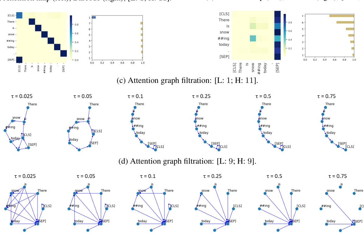
Figure 1: An example of attention maps, barcodes, and filtration procedure for the sentence “There is snowing today.”. Model=En-BERT-base (Devlin et al., 2019). Heads=[Layer 1; Head 11] and [Layer 9; Head 9].

图 1: 句子"There is snowing today."的注意力图、条形码和过滤过程示例。模型=En-BERT-base (Devlin et al., 2019)。注意力头=[第1层;第11头]和[第9层;第9头]。

(1) There is snowing today.

(1) 今天下雪了。

First, we compute attention maps for each Transformer head as shown in Figure 1a-1b (left). These two heads follow different attention patterns (Clark et al., 2019): attention to the next token (Figure 1a) and to the [SEP] token (Figure 1b). Next, we represent the map as a weighted graph, and conduct the filtration procedure for a fixed set of attention weight thresholds. The edges lower than each given threshold are discarded, which results in a set of six attention graphs with their maximum spanning trees (MSTs) becoming a chain (Figure 1c; $\tau{=}0.1$ ), and a star (Figure 1d; $\tau{=}0.5$ ). The families of attention graphs are used to compute persistent features (§3.2).

首先，我们为每个Transformer头计算注意力图，如图1a-1b(左)所示。这两个头遵循不同的注意力模式(Clark等人，2019)：关注下一个token(图1a)和[SEP] token(图1b)。接着，我们将注意力图表示为加权图，并对一组固定的注意力权重阈值进行过滤处理。低于每个给定阈值的边被丢弃，从而得到六组注意力图，其最大生成树(MST)分别形成链状(图1c；$\tau{=}0.1$)和星状(图1d；$\tau{=}0.5$)。这些注意力图族用于计算持久特征(§3.2)。

Figure 1a-1b (right) depict barcodes for each family of graphs. The bars are sorted by length. The number of bars equals $|T|-1$ , where $|T|$ is the number of tokens in the input sentence. The bars in yellow correspond to the 0-dimensional features acquired from the edges of the MST. The bars in blue refer to 1-dimensional features, which stand for non-trivial simple cycles. Such cycle appears in the first family (Figure 1c; $_{\tau=0.05}$ ), which is shown as a blue bar in Figure 1a. By contrast, there are no cycles in the second family (Figure 1d) and on the corresponding barcode.

图 1a-1b (右)展示了每个图族的条形码。条形按长度排序，条数等于$|T|-1$，其中$|T|$是输入句子的token数量。黄色条形对应从最小生成树(MST)边获取的0维特征，蓝色条形代表1维特征(即非平凡简单环)。这种环出现在第一图族(图1c；$_{\tau=0.05}$)，对应图1a中的蓝色条形。相比之下，第二图族(图1d)及其对应条形码中不存在环。

3.2 Persistent Features of Attention Graphs

3.2 注意力图的持久性特征

We follow Kushnareva et al. (2021) to design three groups of persistent features of the attention graph: (i) topological features, (ii) features derived from barcodes, and (iii) features based on distance to attention patterns. The features are computed on attention maps produced by a Transformer LM.

我们遵循Kushnareva等人(2021)的方法，设计了注意力图的三大类持久性特征：(i)拓扑特征，(ii)从条形码(barcode)衍生的特征，以及(iii)基于与注意力模式距离的特征。这些特征是在Transformer语言模型生成的注意力图上计算的。

Topological Features. Topological features include the first two Betti numbers of the undirected graph $\beta_{0}$ and $\beta_{1}$ and standard properties of the directed graph, such as the number of strongly connected components, edges, and cycles. The features are calculated on pre-defined thresholds over undirected and directed attention graphs from each head separately and further concatenated.

拓扑特征。拓扑特征包括无向图的前两个贝蒂数$\beta_{0}$和$\beta_{1}$，以及有向图的标准属性，如强连通分量、边和环的数量。这些特征是在预定义的阈值上分别对每个头的无向和有向注意力图进行计算，并进一步拼接而成。

Features Derived from Barcodes. Barcode is the representation of the graph’s persistent homology (Barannikov, 2021). We use the Ripser+ $^+$ toolkit (Zhang et al., 2020) to compute $0/1.$ - dimensional barcodes for $A^{a t t n}$ . Since Ripser $^{++}$ leverages upon distance matrices, we transform $A^{a t t n}$ as $A^{\prime}=1-\operatorname*{max}\left(A^{a t t n},A^{a t t n T}\right)$ .

从条形码中提取的特征。条形码是图持久同调的表现形式 (Barannikov, 2021)。我们使用 Ripser+ $^+$ 工具包 (Zhang et al., 2020) 计算 $A^{a t t n}$ 的 $0/1.$ 维条形码。由于 Ripser $^{++}$ 基于距离矩阵运算，我们将 $A^{a t t n}$ 转换为 $A^{\prime}=1-\operatorname*{max}\left(A^{a t t n},A^{a t t n T}\right)$。

Next, we compute descriptive characteristics of each barcode, such as the sum/average/variance of lengths of bars, the number of bars with the time of birth/death greater/lower than a threshold, and the entropy of the barcodes. The sum of lengths of bars $(H_{0}S)$ corresponds to the 0-dimensional barcode and represents the sum of edge weights in the $A^{\prime\prime}\mathrm{s}$ minimum spanning tree. The average length of bars $(H_{0}M)$ corresponds to the mean edge weight in this tree, i.e. $H_{0}M=1-$ (the mean edge weight of the maximum spanning tree in $A^{a t t n}$ ).

接下来，我们计算每个条形码的描述性特征，例如条带长度的总和/平均值/方差、出生/死亡时间大于/小于阈值的条带数量，以及条形码的熵。条带长度总和 $(H_{0}S)$ 对应0维条形码，表示 $A^{\prime\prime}\mathrm{s}$ 最小生成树中的边权重总和。条带平均长度 $(H_{0}M)$ 对应该树的平均边权重，即 $H_{0}M=1-$ ( $A^{a t t n}$ 中最大生成树的平均边权重 ) 。

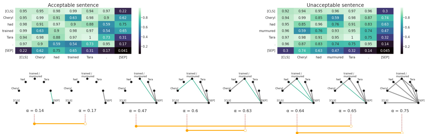
Figure 2: A graphical representation of RTD-barcodes. In the top row given $A^{\prime}$ matrices derived from attention maps for acceptable and unacceptable sentences. Edges present in both graphs $G_{a}^{\alpha_{i}}$ and $G_{b}^{\alpha_{i}}$ at a given threshold $\alpha_{i}$ are colored in grey. Edges present only in graph $G_{b}^{\alpha_{i}}$ are colored in green.

图 2: RTD条形码的图形化表示。顶行展示了从可接受与不可接受句子的注意力图导出的$A^{\prime}$矩阵。在给定阈值$\alpha_{i}$下，同时存在于图$G_{a}^{\alpha_{i}}$和图$G_{b}^{\alpha_{i}}$中的边以灰色显示，仅存在于图$G_{b}^{\alpha_{i}}$中的边以绿色显示。

Features Based on Distance to Patterns. The shape of attention graphs can be divided into several patterns: attention to the previous/current/next token, attention to the [SEP]/[CLS] token, and attention to punctuation marks (Clark et al., 2019). We formalize attention patterns by binary matrices and calculate distances to them as follows. We take the Frobenius norm of the difference between the matrices normalized by the sum of their norms. The distances to patterns are used as a feature vector.

基于模式距离的特征。注意力图形态可分为若干模式：关注前一个/当前/后一个token、关注[SEP]/[CLS]token、关注标点符号 (Clark et al., 2019)。我们通过二元矩阵形式化注意力模式，并按如下方式计算其距离：取矩阵差值的Frobenius范数（经范数之和归一化）。模式距离被用作特征向量。

Notations. We summarize the notations used throughout the paper:

符号说明。我们总结了本文中使用的符号：

• $H_{i}$ : $i$ -th Homology Group • $\beta_{i}$ : Betti number, dimension of $H_{i}$ • $H_{0}S$ : The sum of lengths of bars • $H_{0}M$ : The average of lengths of bars • $P C A$ : Principal Component Analysis • $P C^{{i}}$ : Subset ${i}$ of principal components • MST : Maximum Spanning Tree • RTD: Representation Topology Divergence

• $H_{i}$: 第$i$个同调群
• $\beta_{i}$: 贝蒂数 (Betti number)，$H_{i}$的维度
• $H_{0}S$: 条形长度之和
• $H_{0}M$: 条形长度的平均值
• $PCA$: 主成分分析 (Principal Component Analysis)
• $PC^{{i}}$: 主成分子集${i}$
• MST: 最大生成树 (Maximum Spanning Tree)
• RTD: 表示拓扑分歧 (Representation Topology Divergence)

3.3 Representation Topology Divergence

3.3 表示拓扑差异 (Representation Topology Divergence)

Representation Topology Divergence (RTD; Barannikov et al., 2022) measures topological dissimilarity between a pair of weighted graphs with oneto-one vertex correspondence. Figure 2 outlines computation of RTD for a sentence pair in Exam

表征拓扑差异 (Representation Topology Divergence, RTD; Barannikov等, 2022) 用于衡量具有顶点一一对应关系的两个加权图之间的拓扑差异。图2展示了示例中句子对的RTD计算过程。

ple (2).

(2) a. Cheryl had trained Tara. b. *Cheryl had murmured Tara.

(2) a. Cheryl 训练过 Tara。 b. *Cheryl 曾低声对 Tara 说话。

First, we compute attention maps for the input sentences $S_{a}$ and $S_{b}$ with a Transformer LM, and represent them as the weighted graphs $G_{a}$ and $G_{b}$ . Next, we establish a one-to-one match between the vertices, and sort the filtration s $G_{a}^{\alpha_{i}}$ and $G_{b}^{\alpha_{i}}$ with $\alpha{=}1-\tau$ in the ascending order. We then track the hierarchical formation of connected components in the graph $G_{a}^{\alpha_{i}}\cap G_{b}^{\alpha_{i}}$ while increasing $\alpha_{i}$ . The $\mathrm{\calRTD}(G_{a},G_{b})$ feature appears at threshold $\alpha_{i}$ if an edge with the weight $\alpha_{i}$ in the graph $G_{b}$ joins two different connected components of the graph $G_{a}^{\alpha_{i}}\cap G_{b}^{\alpha_{i}}$ . This feature disappears at the threshold $\alpha_{j}$ if the two $G_{a}^{\alpha_{i}}\cap G_{b}^{\alpha_{i}}$ connected components become joined in the graph $G_{a}^{\alpha_{j}}$ .

首先，我们使用Transformer LM计算输入句子$S_{a}$和$S_{b}$的注意力图，并将其表示为加权图$G_{a}$和$G_{b}$。接着，我们在顶点之间建立一一对应关系，并按升序对过滤后的图$G_{a}^{\alpha_{i}}$和$G_{b}^{\alpha_{i}}$进行排序，其中$\alpha{=}1-\tau$。然后，在逐步增加$\alpha_{i}$的过程中，我们追踪图$G_{a}^{\alpha_{i}}\cap G_{b}^{\alpha_{i}}$中连通分量的层次形成情况。如果在图$G_{b}$中权重为$\alpha_{i}$的边连接了图$G_{a}^{\alpha_{i}}\cap G_{b}^{\alpha_{i}}$的两个不同连通分量，则$\mathrm{\calRTD}(G_{a},G_{b})$特征会在阈值$\alpha_{i}$处出现。如果这两个$G_{a}^{\alpha_{i}}\cap G_{b}^{\alpha_{i}}$连通分量在图$G_{a}^{\alpha_{j}}$中合并，则该特征会在阈值$\alpha_{j}$处消失。

Example. We can identify the “birth” of the RTD feature at $\alpha{=}0.47$ , when an edge appears in $G_{b}^{\alpha=0.47}$ between the connected component “trained/murmured” and the connected component with four vertices, namely “[SEP]”, “[CLS]”, “.”, and “Tara” (Figure 2; the appearing edge is colored in green). We observe its “death”, when the edge becomes present in both attention graphs at $\alpha{=}0.65$ (the corresponding edge changes its color to grey in the graph $G_{a}^{\bar{\alpha}=0.65}\cap G_{b}^{\alpha=0.65}.$ ). When comparing the graphs in this manner, we can associate a lifetime to the feature by computing the difference between the moments of its “death” (e.g., $\alpha_{j}{=}0.65)$ and “birth” (e.g., $\alpha_{i}{=}0.47)$ . The lifetimes are illustrated as the orange bars $[\alpha_{i},\alpha_{j}]$ in Figure 2. The resulting value of $\mathsf{R T D}(G_{a},G_{b})$ is the sum of lifetimes $\alpha_{j}-\alpha_{i}$ over all such features. A formal description of RTD is provided in Appendix A.

示例。我们可以在$\alpha{=}0.47$时识别RTD特征的"诞生"，此时$G_{b}^{\alpha=0.47}$中在连通分量"trained/murmured"与包含四个顶点("[SEP]","[CLS]",".","Tara")的连通分量之间出现了一条边(图2；新出现的边显示为绿色)。当该边在$\alpha{=}0.65$时同时出现在两个注意力图中(对应边在$G_{a}^{\bar{\alpha}=0.65}\cap G_{b}^{\alpha=0.65}$中变为灰色)，我们观察到该特征的"消亡"。通过这种方式比较图结构，我们可以通过计算特征"消亡"(如$\alpha_{j}{=}0.65$)与"诞生"(如$\alpha_{i}{=}0.47$)时刻的差值来确定其特征生命周期。这些生命周期在图2中显示为橙色区间$[\alpha_{i},\alpha_{j}]$。$\mathsf{R T D}(G_{a},G_{b})$的最终值是所有这些特征生命周期$\alpha_{j}-\alpha_{i}$的总和。RTD的形式化定义详见附录A。

4 Acceptability Classification

4 可接受性分类

4.1 Data

4.1 数据

We use three LA classification benchmarks in English (COLA; Warstadt et al., 2019), Italian (ITACOLA; Trotta et al., 2021) and Swedish (DALAJ; Volodina et al., 2021). COLA and ITACOLA contain sentences from linguistic textbooks and cover morphological, syntactic, and semantic phenomena. The target labels are the original authors’ acceptability judgments. DALAJ includes L2-written sentences with morphological violations or incorrect word choices. The benchmark statistics are described in Table 1 (see Appendix C). We provide examples of acceptable and unacceptable sentences in English (3), Italian (4), and Swedish (5) from the original papers.

我们使用了三个英语 (COLA; Warstadt等人, 2019)、意大利语 (ITACOLA; Trotta等人, 2021) 和瑞典语 (DALAJ; Volodina等人, 2021) 的语言可接受性分类基准。COLA和ITACOLA包含来自语言学教材的句子，涵盖形态、句法和语义现象，目标标签是原作者的可接受性判断。DALAJ包含存在形态违规或用词错误的二语写作句子。基准统计数据如表 1 所示 (见附录C)。我们从原始论文中选取了英语 (3)、意大利语 (4) 和瑞典语 (5) 的可接受与不可接受句子示例。

4.2 Models

4.2 模型

We run the experiments on the following Transformer LMs: En-BERT-base (Devlin et al., 2019), It-BERT-base (Schweter, 2020), Sw-BERT- base (Malmsten et al., 2020), and XLM-Rbase (Conneau et al., 2020). Each LM has two instances: frozen (a pre-trained model with frozen weights), and fine-tuned (a model fine-tuned for LA classification in the corresponding language).

我们在以下Transformer模型上进行了实验：En-BERT-base (Devlin et al., 2019)、It-BERT-base (Schweter, 2020)、Sw-BERT-base (Malmsten et al., 2020)和XLM-Rbase (Conneau et al., 2020)。每个模型包含两种实例：冻结权重(frozen)的预训练模型，以及针对相应语言进行LA分类任务微调(fine-tuned)的模型。

Baselines. We use the fine-tuned LMs, and a linear layer trained over the pooler output from the frozen LMs as baselines.

基线方法。我们使用微调后的语言模型(LMs)，以及在冻结语言模型的池化输出(pooler output)上训练的线性层作为基线。

Our Models. We train Logistic Regression classifiers over the persistent features computed with each model instance: $(i)$ the average length of bars $(H_{0}M)$ ; (ii) concatenation of all topological features referred to as TDA (§3.2). Following Warstadt et al., we evaluate the performance with the accuracy score (Acc.) and Matthew’s Correlation Co

我们的模型。我们在每个模型实例计算的持久特征上训练逻辑回归分类器：(i) 柱状图的平均长度 $(H_{0}M)$；(ii) 所有拓扑特征的拼接，称为TDA（见3.2节）。遵循Warstadt等人的方法，我们使用准确率（Acc.）和马修斯相关系数（Matthew’s Correlation Co）评估性能。

模型	冻结语言模型		分布外数据/测试集 Acc.MCC		微调语言模型 Acc.MCC		分布内数据/开发集分布外数据/测试集
CoLA
En-BERT	69.6	0.037	69.0	0.082	83.1 0.580	81.0	0.536
En-BERT+HOM	75.0	0.338	75.2	0.372	85.2	0.635 81.2	0.542
En-BERT+TDA	77.2	0.420	76.7	0.420	88.6 0.725	82.1	0.565
XLM-R	68.9	0.041	68.6	0.072	80.8 0.517	79.3	0.489
XLM-R+HOM	71.3	0.209	69.8	0.187	81.2 0.532	77.7	0.445
XLM-R + TDA	73.0	0.336	70.3	0.297	86.9 0.683	80.4	0.522
ItaCoLA
It-BERT	81.1	0.032	82.1	0.140	87.4 0.351	86.8	0.382
It-BERT+HOM	85.0	0.124	83.6	0.055	87.0 0.361	85.7	0.370
It-BERT + TDA	89.2	0.478	85.8 0.352	91.1	0.597	86.4	0.424
XLM-R	85.4	0.000	84.2 0.000	85.7	0.397	85.6	0.434
XLM-R+ H0M	84.7	0.095	83.3 0.072	86.9	0.370	86.6	0.397
XLM-R + TDA	88.3	0.411	84.4	0.208 92.8	0.683	86.1	0.398
DaLAJ
Sw-BERT	58.3	0.183	59.0	0.188	71.9	0.462	74.2 0.500
Sw-BERT+HOM	69.3	0.387	58.4	0.169	76.9 0.542	68.7	0.375
Sw-BERT+TDA	62.1	0.243	64.4	0.289	71.8 0.442	73.4	0.478
XLM-R	52.2	0.069	51.5	0.038	60.6 0.243	62.8	0.297
XLM-R+ H0M	61.1	0.224	61.8	0.237	62.5 0.256	64.5	0.295
XLM-R + TDA	51.1	0.227	54.1	0.218	62.5 0.255	65.5	0.322

Table 1: Acceptability classification results by benchmark. $\mathbf{ID}\mathbf{D}{=}^{\circ}$ “in domain dev” set (COLA). OODD $\vDash^{\epsilon}$ “out of domain dev” set (COLA). Dev; Test=dev and test sets in ITACOLA and DALAJ. The best score is put in bold, the second best score is underlined.

表 1: 各基准测试的 acceptability 分类结果。$\mathbf{ID}\mathbf{D}{=}^{\circ}$ 表示 "in domain dev" 集 (COLA)。OODD $\vDash^{\epsilon}$ 表示 "out of domain dev" 集 (COLA)。Dev; Test=ITACOLA 和 DALAJ 中的开发集和测试集。最佳分数加粗显示，次佳分数加下划线。

efficient (MCC; Matthews, 1975). The fine-tuning details are provided in Appendix B.

高效 (MCC; Matthews, 1975)。微调细节详见附录B。

4.3 Results

4.3 结果

Table 1 outlines the LA classification results. Our $T D A$ class if i ers generally outperform the baselines by up to $\mathrm{0.14MCC}$ for English, $\mathrm{0.24MCC}$ for Italian, and $\mathrm{0.08MCC}$ for Swedish. The $H_{0}M$ feature can solely enhance the performance for English and Italian up to 0.1, and concatenation of all features receives the best scores. Comparing the results under the frozen and fine-tuned settings, we draw the following conclusions. The TDA features significantly improve the frozen baseline performance but require the LM to be fine-tuned for maximizing the performance. However, the $T D A/H_{0}M$ classifiers perform on par with the fine-tuned baselines for Swedish. The results suggest that our features may fail to infer lexical items and word derivation violations peculiar to the DALAJ benchmark.

表1: 概述了LA分类结果。我们的TDA分类器在英语上最高提升0.14MCC，意大利语提升0.24MCC，瑞典语提升0.08MCC，整体优于基线模型。H0M特征单独使用可将英语和意大利语性能提升最高达0.1，而所有特征的组合能获得最佳分数。通过对比冻结参数和微调设置的实验结果，我们得出以下结论：TDA特征能显著提升冻结基线的性能，但需要微调语言模型以实现最大性能提升。不过对于瑞典语，TDA/H0M分类器与微调基线表现相当。这些结果表明，我们的特征可能无法有效推断DALAJ基准测试中特有的词汇项和构词违规情况。

Effect of Freezing Layers. Another finding is that freezing the Transformer layers significantly affects acceptability classification. Most of the frozen baselines score less than $0.1~\mathrm{MCC}$ across all languages. The results align with Lee et al. (2019), who discuss the performance degradation of BERT-based models depending upon the number of frozen layers. With all layers frozen, the model performance can fall to zero.

冻结层数的影响。另一个发现是冻结Transformer层会显著影响可接受性分类效果。在所有语言中，大多数冻结基线的得分都低于$0.1~\mathrm{MCC}$。该结果与Lee等人(2019)的研究一致，他们讨论了基于BERT的模型性能会随冻结层数增加而下降。当所有层都被冻结时，模型性能可能降至零。

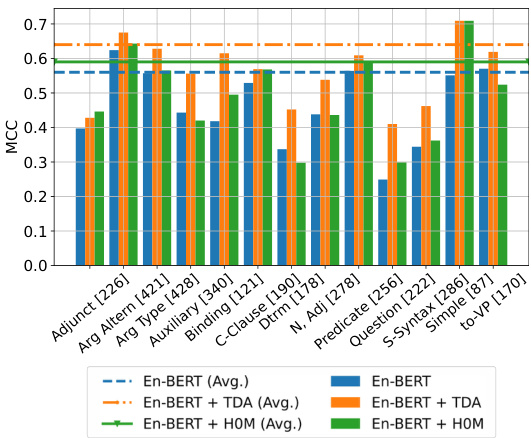
Figure 3: Performance (MCC) of the fine-tuned EnBERT and XLM-R by major linguistic feature. Average MCC scores are represented with dashed lines. The number of sentences including the feature is placed in square brackets.

图 3: 按主要语言特征细调的EnBERT和XLM-R性能(MCC)。虚线表示平均MCC分数。包含该特征的句子数量标注在方括号中。

Results by Linguistic Features. We run a diagnostic evaluation of the fine-tuned models using a grammatically annotated version of the COLA development set (Warstadt and Bowman, 2019). Figure 3 (En-BERT and XLM-R; Figure 1 in Appendix C.1) present the results of measuring the MCC of the sentences including the major features.

基于语言特征的实验结果。我们使用经过语法标注的COLA开发集(Warstadt and Bowman, 2019)对微调模型进行诊断性评估。图3(En-BERT和XLM-R；附录C.1中的图1)展示了包含主要特征的句子MCC测量结果。

The overall pattern is that the TDA class if i ers may outperform the fine-tuned baselines, while the $H_{0}M$ ones perform on par with the latter. The per- formance is high on sentences with default syntax (Simple) and marked argument structure, including prepositional phrase arguments (Arg. Type), and verb phrases with unusual structures (Arg. Altern). The $T D A$ features capture surface properties, such as presence of auxiliary or modal verbs (Auxiliary), and structural ones, e.g., embedded complement clauses (Comp Clause) and infinitive constructions (to-VP). The models receive moderate MCC scores on sentences with question-like properties (Question), adjuncts performing semantic functions (Adjunct), negative polarity items, and comparative constructions (Determiner).

整体模式表现为：TDA 分类器可能优于微调基线模型，而 $H_{0}M$ 类模型与后者表现相当。在默认句法结构（Simple）、带标记论元结构（包括介词短语论元 (Arg. Type) 和特殊结构动词短语 (Arg. Altern)）的句子上表现优异。$T D A$ 特征能捕捉表层属性（如助动词或情态动词的存在 (Auxiliary)）和结构属性（例如嵌入式补语从句 (Comp Clause) 和不定式结构 (to-VP)）。模型在具有疑问句特性 (Question)、执行语义功能的附加语 (Adjunct)、否定极性项和比较结构 (Determiner) 的句子上获得中等MCC分数。

Analysis of the Feature Space. The LA classification experiments are conducted in the sparse feature space, where the TDA features can strongly correlate with one another, and their contribution is unclear. We run a complementary experiment to understand better how linguistic features are modeled with topology. We investigate the feature space with dimensionality reduction (principal component analysis, PCA; Pearson, 1901) by interpreting components’ structure and identifying the feature importance to the classifier’s predictions using Shapley values (Shapley, 1953), a game-theoretic approach to the attribution problem (Sun dara rajan and Najmi, 2020). Appendix C.2 describes the experiment on the fine-tuned En-BERT $+T D A$ model using the grammatically annotated COLA development set.

特征空间分析。LA分类实验在稀疏特征空间中进行，其中TDA特征之间可能存在强相关性，且其贡献尚不明确。我们通过补充实验来进一步理解如何用拓扑结构建模语言特征。采用降维方法（主成分分析，PCA；Pearson, 1901）研究特征空间，通过解释主成分结构并结合博弈论归因方法Shapley值（Shapley, 1953）(Sun dara rajan and Najmi, 2020)来识别特征对分类器预测的重要性。附录C.2描述了基于语法标注COLA开发集对微调后的En-BERT $+T D A$ 模型开展的实验。

The results show that (i) features of the higherlayer heads, such as the average vertex degree, the number of connected components, edges, and cycles, and attention to the current token, contribute most to the major linguistic features. (ii) Attention to the [CLS]/next token is important to the Determiner, Arg. Type, Comp Clause, and to-VP properties, while attention to the first token and punctuation marks has the least effect in general. (iii) The number of nodes influences the classifier behavior, which is in line with Warstadt and Bowman, who discuss the effect of the sentence length on the performance.

结果表明：(i) 高层注意力头(head)的特征（如平均顶点度数、连通组件数量、边与环的数量、对当前token的关注度）对主要语言特征贡献最大。(ii) 对[CLS]/下一token的关注度对限定词(Determiner)、论元类型(Arg. Type)、补语从句(Comp Clause)和不定式动词短语(to-VP)属性具有重要影响，而对首token和标点符号的关注度总体影响最小。(iii) 节点数量会影响分类器行为，这与Warstadt和Bowman讨论的句子长度对性能的影响一致[20]。

5 Linguistic Minimal Pairs

5 语言学最小对立对

5.1 Data

5.1 数据

BLIMP (Benchmark of Linguistic Minimal Pairs; Warstadt et al., 2020a) evaluates the sen- sitivity of LMs to acceptability contrasts in terms of a forced choice between minimal pairs, as in Example (6). The benchmark consists of 67 pair types, each including 1k pairs covering 12 language phenomena in morphology, syntax, and semantics.

BLIMP（语言最小对比基准测试；Warstadt等人，2020a）通过强制选择最小对比对（如示例(6)）来评估大语言模型对可接受性对比的敏感度。该基准包含67种对比类型，每种涵盖形态、句法和语义等12种语言现象的1000组对比对。

(6) a. Whose hat should Tonya wear? b. *Whose should Tonya wear hat?

(6) a. Tonya应该戴谁的帽子？ b. *Tonya应该戴谁的帽子？

5.2 Models

5.2 模型

We conduct the experiments using two Transformer LMs for English: BERT-base and RoBERTabase (Liu et al., 2019).

我们使用两个针对英语的Transformer语言模型进行实验：BERT-base和RoBERTabase (Liu et al., 2019)。

Baselines. We compare our methods with the results on BLIMP for human annotators and nine LMs (Warstadt et al., 2020a; Salazar et al., 2020). The baselines range from statistical N-gram LMs to Transformer LMs.

基线方法。我们将自身方法与BLIMP数据集上的人类标注结果及九种语言模型 (Warstadt et al., 2020a; Salazar et al., 2020) 进行对比，基线方法涵盖统计N元语言模型至Transformer语言模型。

Our Models. Given a minimal pair as in Example (2), we build attention graphs $G_{a}$ and $G_{b}$ from each attention head of a frozen Transformer LM. We use the $H_{0}M$ feature (§3.2) and RTD (§3.3) as scoring functions to distinguish between the sentences $S_{a}$ and $S_{b}$ . The scoring is based on empirically defined decision rules modeled after the forced-choice task:

我们的模型。给定如示例(2)中的最小对比对，我们从冻结的Transformer LM的每个注意力头构建注意力图$G_{a}$和$G_{b}$。我们使用$H_{0}M$特征(§3.2)和RTD(§3.3)作为评分函数来区分句子$S_{a}$和$S_{b}$。评分基于根据强制选择任务建模的经验定义决策规则:

We evaluate the scoring performance of each attention head, head ensembles, and all heads w.r.t. each and all linguistic phenomena in BLIMP. The following head configurations are used for each Transformer LM and scoring function:

我们评估了每个注意力头、注意力头组合以及所有注意力头在BLIMP中针对每种及所有语言现象的打分表现。针对每个Transformer语言模型和打分函数，采用了以下注意力头配置：

• Phenomenon Head and Top Head are the bestperforming attention heads for each and all phenomena, respectively. The heads undergo the selection with a brute force search and operate as independent scorers. • Head Ensemble is a group of the bestperforming attention heads selected with beam search. The size of the group is always odd. We collect majority vote scores from attention heads in the group. • All Heads involves majority vote scoring with all 144 heads. We use random guessing in case of equality of votes. This setup serves as a proxy for the efficiency of the head selection.

• Phenomenon Head 和 Top Head 分别是针对每种现象和所有现象表现最佳的注意力头。这些头通过暴力搜索进行选择，并作为独立评分器运行。
• Head Ensemble 是通过束搜索选出的表现最佳的一组注意力头。该组的大小始终为奇数。我们从组内的注意力头中收集多数投票分数。
• All Heads 涉及使用全部 144 个头进行多数投票评分。在票数相等时采用随机猜测。此设置作为头选择效率的代理指标。

Notes on Head Selection. Recall that the head selection procedure3 imposes the following limitation. Auxiliary labeled minimal pairs are required to find the best-performing Phenomenon, Top Heads, and Head Ensembles. However, this procedure is more optimal and beneficial than All Heads since it maximizes the performance when utilizing only one or 9-to-59 heads. We also analyze the effect of the amount of auxiliary data used for the head selection on the scoring performance (§5.3). Appendix D.1 presents a more detailed description of the head selection procedure.

头选择注意事项。回顾头选择过程3存在以下限制：需要辅助标记的最小对来寻找表现最佳的现象(Phenomenon)、顶部头(Top Heads)和头集成(Head Ensembles)。但该过程比全头(All Heads)更优且有益，因为仅使用1个或9至59个头时能最大化性能。我们还分析了用于头选择的辅助数据量对评分性能的影响(§5.3)。附录D.1提供了头选择过程的更详细说明。

5.3 Results

5.3 结果

We provide the results of scoring BLIMP pairs in Table 2. The accuracy is the proportion of the minimal pairs in which the method prefers an acceptable sentence to an unacceptable one. We report the maximum accuracy scores for our methods across five experiment restarts. The general trends are that the best head configuration performs on par with the human baseline and achieves the high- est overall performance (RoBERTa-base $^+$ RTD; Head Ensemble). RoBERTa predominantly surpasses BERT and other baselines, and topological scoring may improve on scores from both BERT and RoBERTa for particular phenomena.

我们在表2中提供了BLIMP配对评分的结果。准确率是指该方法在最小配对中偏好可接受句子而非不可接受句子的比例。我们报告了五次实验重启中方法的最高准确率分数。总体趋势表明，最佳头部配置与人类基线表现相当，并达到最高整体性能 (RoBERTa-base $^+$ RTD; Head Ensemble)。RoBERTa主要超越BERT和其他基线，而拓扑评分可能针对特定现象改进BERT和RoBERTa的分数。

Top Head Results. We find that $H_{0}M/\mathrm{RTD}$ scoring with only one Top Head overall outperforms majority voting of 144 heads (All Heads) by up to $10.6%$ and multiple baselines by up to $20.7%$ (5- gram, LSTM, Transformer-XL, GPT2-large). However, this head configuration performs worse than masked LM scoring (Salazar et al., 2020) for BERTbase (by $8.8%$ ; Top Head=[8; 0]) and RoBERTa- base (by $4.6%$ ; Top Head=[11; 10]).

顶级头部结果。我们发现仅使用一个顶级头部的 $H_{0}M/\mathrm{RTD}$ 评分方法在整体上优于144个头部（所有头部）多数投票（All Heads），最高提升 $10.6%$，并且优于多个基线方法（5-gram、LSTM、Transformer-XL、GPT2-large），最高提升 $20.7%$。然而，这种头部配置在BERTbase（下降 $8.8%$；Top Head=[8; 0]）和RoBERTa-base（下降 $4.6%$；Top Head=[11; 10]）上的表现不如掩码语言模型评分（Salazar et al., 2020）。

Phenomenon Head Results. We observe that the $H_{0}M/\mathrm{TDA}$ scoring performance of Phenomenon Heads insignificantly differ for the same model. Phenomenon Heads generally receive higher scores than the corresponding Top Heads for BERT/RoBERTa (e.g., Binding: $+17.1/+5.8%$ ; Quantifiers: $+17.7/+5.0%$ ; Det.- Noun agr: $+13.0/+1.7%\rangle$ , and perform best or second-best on Binding and Ellipsis. Their overall performance further adds up to $6.4/6.0%$ and is comparable with Salazar et al.. The results indicate that heads encoding the considered phenomena are distributed at the same or nearby layers, namely [3; 6-9; 11] (BERT), and [2-3; 8-11] (RoBERTa).

现象头结果。我们观察到，同一模型中现象头的 $H_{0}M/\mathrm{TDA}$ 评分表现差异不显著。对于BERT/RoBERTa，现象头通常比对应的Top Heads获得更高分数（例如：绑定(Binding): $+17.1/+5.8%$；量词(Quantifiers): $+17.7/+5.0%$；限定词-名词一致(Det.-Noun agr): $+13.0/+1.7%\rangle$，且在绑定和省略(Ellipsis)任务上表现最佳或次佳。其整体性能进一步提升至 $6.4/6.0%$，与Salazar等人的研究相当。结果表明，编码这些现象的头部分布在相同或邻近的层，即BERT的[3; 6-9; 11]层和RoBERTa的[2-3; 8-11]层。

Head Ensemble Results. Table 3 describes the most optimal Head Ensembles by Transformer LM. Most heads selected under the $H_{0}M$ and RTD scoring functions are similar w.r.t. LMs. While the selected BERT heads are distributed across all layers, the RoBERTa ones tend to be localized at the middle-to-higher layers. Although RoBERTa utilizes smaller ensembles when delivering the best overall score, some heads contribute in both LMs, most notably at the higher layers.

头集成结果。表3描述了Transformer LM最优的头集成。在$H_{0}M$和RTD评分函数下选择的大多数头对于LMs来说是相似的。虽然选择的BERT头分布在所有层中，但RoBERTa的头往往集中在中高层。尽管RoBERTa在提供最佳总体分数时使用了较小的集成，但某些头在两种LMs中都有贡献，尤其是在较高层。

Overall, the RoBERTa $H_{0}M/\mathrm{RTD}$ ensembles get the best results on Filler gap, Quantifiers, Island effects, NPI, and $S{-}V$ agr as shown in Table 2, matching the human level and surpassing four larger LMs on all phenomena by up to $7.4%$ (GPT2- medium and GPT2/BERT/RoBERTa-large).

总体而言，RoBERTa $H_{0}M/\mathrm{RTD}$ 集成模型在填充间隙 (Filler gap) 、量词 (Quantifiers) 、孤岛效应 (Island effects) 、否定极性项 (NPI) 以及 $S{-}V$ 一致性任务中取得了最佳结果（如表 2 所示），达到人类水平，并在所有语言现象上以最高 $7.4%$ 的优势超越 GPT2-medium、GPT2/BERT/RoBERTa-large 四个更大的大语言模型。

模型	总体	分析一致性	论元结构	约束	控制/提升	名数一致性	省略	填充词	不规则	孤岛	NPI	量化	主谓一致性
Warstadt et al. (2020a)
5-gram	61.2	47.9	71.9	64.4	68.5	70.0	36.9	60.2	79.5	57.2	45.5	53.5	60.3
LSTM	69.8	91.7	73.2	73.5	67.0	85.4	67.6	73.9	89.1		46.6	51.7	64.5
Transformer-XL	69.6	94.1	72.2	74.7	71.5	83.0	77.2	66.6		78.2	48.4	55.2	69.3
GPT2-large	81.5	99.6	78.3	80.1	80.5	93.3	86.6	81.3		84.1	70.6	78.9	71.3
人类基线	88.6	97.5	90.0	87.3	83.9	92.2	85.0	86.9	97.0		84.9	88.1	86.6
Salazar et al. (2020)
GPT2-medium	82.6	99.4	83.4	77.8	83.0	96.3	86.3	81.3	94.9	71.7	74.7		74.1
BERT-base	84.2	97.0	80.0	82.3	79.6	97.6	89.4	83.1	96.5		73.6	84.7	71.2
BERT-large	84.8	97.2	80.7	82.0	82.7	97.6	86.4	84.3	92.8		77.0	83.4	72.8
RoBERTa-base	85.4	97.3	83.5	77.8	81.9	97.0	91.4	90.1	96.2		80.7	81.0	69.8
RoBERTa-large	86.5	97.8	84.6	79.1	84.1	96.8	90.8	88.9	96.8		83.4	85.5	70.2
BERT-base + HoM
[层; 头]		[8:8]	[0:8]	[7;0]	[8;0]		[7;0]	[7;11]	[9;7]	[6;1]	[11;7]	[8;9]	[3;7]
现象头	81.7	94.9	75.9	80.4	79.2	96.7		89.1	75.9	93.0	70.5	84.6	81.2
顶级头 [8:0] 头集成	75.4	86.8	75.9	63.4	79.2	83.7	72.2		67.3	90.3	70.0	83.1	63.5
所有头	84.3	93.3	79.9	83.5	78.6	96.4	78.4	79.5		93.8	74.4	92.5	81.7
	64.8	79.6	69.1	63.9	62.6	86.2	70.7	47.3		90.7	49.5	61.1	50.0
BERT-base + RTD
[层; 头]	X	[8;3]	[8;0]	[7;0]	[8;0]	[7;0]	[7;11]	[9;7]		[6;1]	[9;7]	[8;9]	[3;7]
现象头	81.8	94.5	75.8	80.4	79.2	96.7	89.1		75.0	93.0	72.2	84.4	81.2
顶级头 [8;0]	75.4	86.8 93.9	75.8 82.5	63.3 85.6	79.2 77.0	83.6 96.3	72.1 88.1	67.3		90.2	70.2	83.1	63.6
头集成所有头	85.8	77.8	68.5	63.2	63.6	86.0		80.7		95.7	77.0	92.5 62.0	83.8 51.2
	65.3						73.4	48.4		91.0	51.3
RoBERTa-base + HoM
[层; 头]	X	[9;5]	[9;8]	[9;5]	[9;6]	[9:0]	[8;4]	[11;10]		[9:6]	[3;5]	[11;5]	[11;3]
现象头	86.5	97.6	79.9	90.5	80.7	91.6	89.9	87.1		95.9	78.9	91.1	83.4
顶级头 [11;10]	81.9	90.1	66.0	84.7	71.7	91.0	86.7	87.1		89.5	76.8	90.7	78.4
头集成	87.8	96.3	79.6	87.6	82.6	93.6	84.9	90.4		94.3	83.0	94.6	80.6
所有头 RoBERTa-base + RTD	74.3	80.6	71.2	78.6	67.8	90.6	89.9	75.5		65.1	73.4	65.1	57.0

Table 2: Percentage accuracy of the baseline models, human baseline, and our methods on BLIMP. Overall is the average across all phenomena. The best score is put in bold, the second best score is underlined.

表 2: 基线模型、人类基线及我们方法在BLIMP上的准确率百分比。Overall为所有现象的平均值。最佳分数加粗显示，次佳分数加下划线。

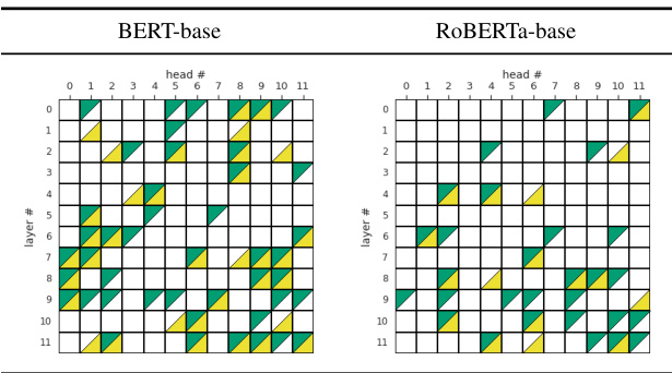
Table 3: Results of selecting the best-performing Head Ensembles with $H_{0}M,$ /RTD-based scoring. $H_{0}M$ heads are colored in green; RTD heads are colored in yellow.

表 3: 基于 $H_{0}M$ /RTD评分选取最佳性能头组合的结果。$H_{0}M$ 头标记为绿色；RTD头标记为黄色。

Effect of Auxiliary Data. Note that the head selection can be sensitive to the number of additional examples. The analysis of this effect is presented in Appendix D.2. The results show that head ensembles, their size, and average performance tend to be more stable when using sufficient examples (the more, the better); however, using only one extra example can yield the performance above $80%$ .

辅助数据的影响。需要注意的是，头部选择对额外样本数量较为敏感。附录D.2对此效应进行了分析，结果表明：当使用充足样本时（越多越好），头部集成方案、其规模及平均性能往往更稳定；但仅使用一个额外样本仍可使性能保持在80%以上。

6 Discussion

6 讨论

Topology and Acceptability. The topological properties of the attention graph represent interpretable and versatile features for judging sentence acceptability and identifying acceptability contrasts in minimal pairs. As one of such properties, the sum length of bars $(H_{0}S)$ — and its normalized version $(H_{0}M)$ — have proved to be efficient for both LA approaches. This simple feature can serve as a profitable input for LA class if i ers and a scoring function to discriminate between minimal pairs. Figure 4 shows an example of the $H_{0}S$ sensitivity to COLA’s question-like properties, such as whmovement out of syntactic islands and matrix and embedded questions. We provide more examples in Appendix E, which demonstrate the distribution shifts between the acceptable and unacceptable sentences.

拓扑结构与可接受性。注意力图的拓扑特性为判断句子可接受性和识别最小对立对中的可接受性对比提供了可解释且通用的特征。其中，条形图总长度 $(H_{0}S)$ 及其标准化版本 $(H_{0}M)$ 已被证明对两种LA方法均有效。这一简单特征可作为LA分类器的有益输入，并作为区分最小对立对的评分函数。图4展示了 $H_{0}S$ 对COLA疑问句特性的敏感性示例，如从句法孤岛提取wh成分、主句与嵌套疑问句等。附录E提供了更多案例，展示可接受句与不可接受句之间的分布差异。

Acceptability Phenomena. The underlying structure of the attention graph encodes various well-established grammatical concepts. We observe that the persistent graph features capture surface properties, morphological agreement, structural relationships, and simple/complex syntactic phenomena well. However, with topology, lexical items, optional syntactic elements, and abstract semantic factors may be difficult to infer. Attention to the first token and punctuation marks contribute least to LA classification, while the other attention pattern features capture various phenomena.

可接受性现象。注意力图的基础结构编码了各种公认的语法概念。我们观察到，持久图特征能较好地捕捉表层属性、形态一致性、结构关系以及简单/复杂句法现象。然而，仅凭拓扑结构、词汇项、可选句法元素和抽象语义因素可能难以推断。对首个token和标点符号的关注对LA分类贡献最小，而其他注意力模式特征则捕捉了多种现象。

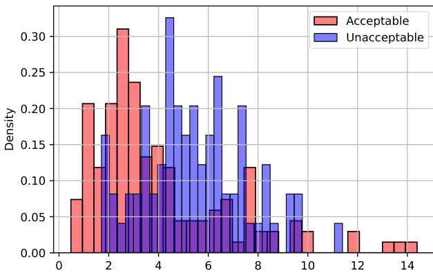
Figure 4: The distribution shift of the $H_{0}S$ feature between the acceptable and unacceptable sentences (Question); [L: 10; H: 0].

图 4: 可接受与不可接受句子间 $H_{0}S$ 特征的分布偏移 (Question); [L: 10; H: 0]。

Linguistic Roles of Heads. Topological tools help gain empirical evidence about the linguistic roles of heads from another perspective. Our findings on the heads’ roles align with several related studies. The results on the COLA-style and BLIMP benchmarks indicate that $(i)$ a single head can perform multiple linguistic functions (Pande et al., 2021), $(i i)$ some linguistic phenomena, e.g., phrasal movement and island effects, are better captured by head ensembles rather than one head (Htut et al., 2019), and $(i i i)$ heads within the same or nearby layers extract similar grammatical phenomena (Bian et al., 2021).

头部的语言学角色。拓扑工具从另一个角度为头部在语言学中的角色提供了实证依据。我们的研究发现与多项相关研究一致：在COLA风格和BLIMP基准测试中，结果表明$(i)$单个头部可执行多种语言功能[20]，$(ii)$某些语言现象（如短语移位和孤岛效应）更适合通过头部组合而非单一头部来捕捉[19]，$(iii)$同一层或邻近层的头部会提取相似的语法现象[21]。

7 Conclusion and Future Work

7 结论与未来工作

Our paper studies the ability of attention heads to judge grammatical acceptability, demonstrating the profitable application of TDA tools to two LA paradigms. Topological features can boost LA classification performance in three typo logically close languages. The $H_{0}M/\mathrm{RTD}$ scoring matches or outperforms larger Transformer LMs and reaches human-level performance on BLIMP, while utilizing 9-to-59 attention heads. We also interpret the correspondence between the persistent features of the attention graph and grammatical concepts, revealing that the former efficiently infer morphological, structural, and syntactic phenomena but may lack lexical and semantic information.

我们的论文研究了注意力头判断语法可接受性的能力，展示了TDA工具在两种LA范式中的有效应用。拓扑特征可以在三种类型学相近的语言中提升LA分类性能。$H_{0}M/\mathrm{RTD}$评分与更大的Transformer大语言模型相当或更优，并在仅使用9至59个注意力头的情况下，在BLIMP上达到人类水平的表现。我们还解释了注意力图的持久特征与语法概念之间的对应关系，揭示了前者能有效推断形态、结构和句法现象，但可能缺乏词汇和语义信息。

In our future work we hope to assess the linguistic competence of Transformer LMs on related resources for typo logically diverse languages and analyze which language-specific phenomena are and are not captured by the topological features. We are also planning to examine novel features, e.g., the number of vertex covers, the graph clique-width, and the features of path homology (Grigor’yan et al., 2020). Another direction is to evaluate the benefits and limitations of the $H_{0}M/\mathrm{RTD}$ features as scoring functions in downstream applications.

在我们未来的工作中，我们希望评估Transformer大语言模型在类型学多样性语言相关资源上的语言能力，并分析哪些语言特定现象能被拓扑特征捕捉或遗漏。我们还计划研究新特征，例如顶点覆盖数、图团宽度以及路径同调特征 (Grigor’yan et al., 2020)。另一个方向是评估$H_{0}M/\mathrm{RTD}$特征作为下游应用评分函数的优势与局限性。

We also plan to introduce support for new deep learning frameworks such as MindSpore4 (Tong et al., 2021) to bring TDA-based experimentation to the wider industrial community.

我们还计划引入对MindSpore4 (Tong et al., 2021) 等新深度学习框架的支持，以便将基于TDA的实验推广至更广泛的工业界。

8 Limitations

8 局限性

8.1 Computational complexity

8.1 计算复杂度

Acceptability classification. Calculation of any topological feature relies on the Transformer’s attention matrices. Hence, the computational complexity of our features is not lower than producing an attention matrix with one head, which is asymptotically $O(n^{2}d+n d^{2})$ given that $n$ is the maximum number of tokens, and $d$ is the token embedding dimension (Vaswani et al., 2017).

可接受性分类。任何拓扑特征的计算都依赖于Transformer的注意力矩阵。因此，我们特征的计算复杂度不低于生成单头注意力矩阵的复杂度，其渐进复杂度为$O(n^{2}d+n d^{2})$，其中$n$表示token的最大数量，$d$表示token嵌入维度 (Vaswani et al., 2017)。

The calculation complexity of the patternbased and threshold-based features is done in linear time $O(e+n)$ , where $e$ is the number of edges in the attention graph. In turn, the number of edges is not higher than $\frac{n(n-1)}{2}\sim n^{2}$ ) n2. The computation of the ${\bf0}^{t h}$ Betti number $\beta_{0}$ takes linear time $O(e+n)$ , as $\beta_{0}$ is equal to the number of the connected components in an undirected graph. The computation of the ${\bf1}^{s t}$ Betti number $\beta_{1}$ takes constant time, since $\beta_{1}=e-n+\beta_{0}$ . The computational complexity of the number of simple cycles and the 1-dimensional barcode features is exponential in the worst case. To reduce the computational burden, we stop searching for simple cycles after a pre-defined amount of them is found.

基于模式和基于阈值的特征计算复杂度为线性时间 $O(e+n)$ ，其中 $e$ 是注意力图中的边数。而边数不超过 $\frac{n(n-1)}{2}\sim n^{2}$ ) n2。计算第 ${\bf0}^{t h}$ 个贝蒂数 $\beta_{0}$ 需要线性时间 $O(e+n)$ ，因为 $\beta_{0}$ 等于无向图中连通分量的数量。计算第 ${\bf1}^{s t}$ 个贝蒂数 $\beta_{1}$ 只需常数时间，因为 $\beta_{1}=e-n+\beta_{0}$ 。简单环数量和1维条形码特征的计算复杂度在最坏情况下是指数级的。为了降低计算负担，我们在找到预定义数量的简单环后停止搜索。

Note that the computational costs could be reduced, e.g., by identifying the most contributing features or the best-performing heads. Consider an example in Figure 5, which illustrates how the COLA performance gets changed depending on the number of En-BERT heads. Here, the head selection is based on a simple procedure. First, we score the attention heads by calculating the maximum correlation between each head’s features and the vector of the target classes on the train set. Second, we train a linear classifier over the $T D A$ features produced by $N$ attention heads ranked by the correlation values, as specified in $\S4.2$ . Satisfactory MCC scores can be achieved when utilizing less than 40 heads with a significant speed up at the inference stage.

请注意，计算成本可以通过识别贡献最大的特征或表现最佳的注意力头来降低。以图 5 为例，它展示了 COLA 性能如何随 En-BERT 注意力头数量的变化而变化。这里的头选择基于一个简单流程：首先，我们通过计算每个头的特征与训练集上目标类别向量之间的最大相关性来对注意力头进行评分；其次，如 $\S4.2$ 所述，我们根据相关性值排序的 $N$ 个注意力头生成的 $T D A$ 特征训练线性分类器。当使用少于 40 个头时，可以在推理阶段显著加速的同时获得令人满意的 MCC 分数。

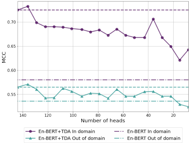
Figure 5: Performance on the COLA development set depending on the number of heads for En-BERT $^+$ $T D A$ .

图 5: En-BERT $^+$ $T D A$ 在COLA开发集上的性能随注意力头数量的变化。

Linguistic Minimal Pairs. Computation of the $H_{0}M$ and RTD features is run via the Ripser $^{++}$ GPU library. Under this library, the minimum spanning tree is found according to Kruskal’s algorithm giving the computational complexity of $H_{0}M$ as $O(n^{2}\log{n})$ . The complexity can be reduced using other algorithms, e.g., Prim’s algorithm, which takes $O(n^{2})$ . The RTD’s computational complexity is more difficult to estimate. RTD is computed via persistence barcodes of dimension 1 for a specific graph with $2n$ vertices. Many optimization techniques and heuristics are implemented in the Ripser $^{++}$ library that significantly reduce the RTD’s complexity.

语言最小对。$H_{0}M$ 和 RTD 特征的计算通过 Ripser$^{++}$ GPU 库运行。在该库中，根据 Kruskal 算法找到最小生成树，得出 $H_{0}M$ 的计算复杂度为 $O(n^{2}\log{n})$。使用其他算法（如 Prim 算法）可将复杂度降至 $O(n^{2})$。RTD 的计算复杂度较难估算，它是通过具有 $2n$ 个顶点的特定图的一维持久条形码计算的。Ripser$^{++}$ 库实现了多种优化技术和启发式方法，可显著降低 RTD 的复杂度。

Empirical estimate. Computing the $H_{0}M/\mathrm{RTD}$ features with 144 BERT heads in the worst case of a 512-token text takes 2.41 and 94.5 sec (NVIDIA Tesla K80 12GB RAM). However, the actual computation time on the considered tasks is empirically more optimal. We provide empirical estimates on the entire BLiMP and LA datasets: 2.4/15.7 hours on BLiMP $\left(H_{0}M/\mathrm{RTD}\right)$ and up to 2 hours on COLA/ITACOLA/DALAJ (estimates by the feature groups: topological features $=24%$ ; features derived from barcode $3=70%$ ; and features based on distance to patterns $=6%$ of the total time).

经验估计。在最坏情况下（512个token的文本），使用144个BERT头计算$H_{0}M/\mathrm{RTD}$特征耗时2.41秒和94.5秒（NVIDIA Tesla K80 12GB显存）。但在实际任务中，计算时间通常更为理想。我们对完整BLiMP和LA数据集进行了经验估计：BLiMP上耗时2.4/15.7小时（$\left(H_{0}M/\mathrm{RTD}\right)$），COLA/ITACOLA/DALAJ上最多2小时（按特征组估算：拓扑特征占总时间24%；条形码3衍生特征占70%；模式距离相关特征占6%）。

8.2 Application Limitations

8.2 应用限制

We also outline several application limitations of our approach. (i) The LA class if i ers require preliminary fine-tuning of Transformer LMs to extract more representative attention graph features and, therefore, achieve better performance. (ii) RTD operates upon a one-to-one vertex correspondence, which may be hindered by tokens segmented into an unequal amount of sub-tokens. As a result, identifying the topological discrepancy between pairs of attention graphs can be restricted in practice, where the graphs are of an arbitrary number of nodes. Regardless of the potential information loss due to sentence truncation in such cases, the RTD heads still receive the best overall score on BLIMP. (iii) The head selection procedure relies on auxiliary data to identify the best-performing head configurations. Annotating the auxiliary data may require additional resources and expertise for practical purposes. However, the procedure maximizes the performance and reduces the computational costs by utilizing less attention heads.

我们还概述了本方法的几项应用限制。(i) LA分类器需要对Transformer语言模型进行初步微调，以提取更具代表性的注意力图特征，从而获得更好的性能。(ii) RTD基于一对一顶点对应关系运行，当token被分割为数量不等的子token时可能受限。因此，在实际应用中识别注意力图对之间的拓扑差异可能受到限制，因为这些图可能具有任意数量的节点。尽管在这种情况下由于句子截断可能导致信息丢失，但RTD头在BLIMP上仍获得了最佳综合评分。(iii) 头选择流程依赖辅助数据来确定最佳性能的头配置。实际应用中，标注辅助数据可能需要额外的资源和专业知识。但该流程通过使用更少的注意力头，既最大化性能又降低了计算成本。

8.3 Linguistic Acceptability

8.3 语言可接受性

Acceptability judgments have been broadly used to investigate whether LMs learn grammatical concepts central to human linguistic competence. However, this approach has several methodological limitations. $(i)$ The judgments may display low reproducibility in multiple languages (Linzen and Oseki, 2018), and (ii) be influenced by an individual’s exposure to ungrammatical language use (Dabrowska, 2010). (iii) Distribution shifts between LMs’ pretraining corpora and LA datasets may introduce bias in the evaluation since LMs tend to assign higher probabilities to frequent patterns and treat them as acceptable in contrast to rare ones (Marvin and Linzen, 2018; Linzen and Baroni, 2021).

可接受性判断被广泛用于研究大语言模型是否学习了人类语言能力的核心语法概念。然而，这种方法存在若干方法论局限：(i) 这些判断在多种语言中可能表现出较低的可复现性 (Linzen and Oseki, 2018)；(ii) 可能受个体接触非规范语言使用的影响 (Dabrowska, 2010)；(iii) 大语言模型预训练语料与语言可接受性数据集之间的分布偏移可能引入评估偏差，因为模型倾向于对高频模式赋予更高概率并将其视为可接受，而低频模式则相反 (Marvin and Linzen, 2018; Linzen and Baroni, 2021)。

9 Ethical Statement

9 伦理声明

Advancing acceptability evaluation methods can improve the quality of natural language generation (Batra et al., 2021). We recognize that this, in turn, can increase the misuse potential of such models, e.g., generating fake product reviews, social media posts, and other targeted manipulation (Jawahar et al., 2020; Weidinger et al., 2021). However, the acceptability class if i ers and scoring functions laid out in this paper are developed for research purposes only. Recall that the topological tools can be employed to develop adversarial defense and artificial text detection models for mitigating the risks (Kushnareva et al., 2021).

提升可接受性评估方法可以改善自然语言生成的质量 (Batra et al., 2021)。我们认识到，这反过来可能增加此类模型的滥用潜力，例如生成虚假产品评论、社交媒体帖子和其他针对性操控 (Jawahar et al., 2020; Weidinger et al., 2021)。然而，本文提出的可接受性分类器和评分函数仅用于研究目的。值得注意的是，拓扑工具可用于开发对抗防御和人工文本检测模型以降低风险 (Kushnareva et al., 2021)。

Acknowledgements

致谢

This work was supported by Ministry of Science and Higher Education grant No. 075-10-2021-068 and by the Mindspore community. Irina Proskurina was supported by the framework of the HSE University Basic Research Program.

本研究由俄罗斯科学与高等教育部资助项目（编号075-10-2021-068）和Mindspore社区支持。Irina Proskurina的研究工作由俄罗斯高等经济大学基础研究计划框架资助。

References

参考文献

Serguei Barannikov. 1994. Framed Morse complexes and its invariants. Adv. Soviet Math., 21:93–115.

Serguei Barannikov. 1994. 框架莫尔斯复形及其不变量. Adv. Soviet Math., 21:93–115.

Serguei Barannikov. 2021. Canonical Forms $=$ Persistence Diagrams. Tutorial. In European Workshop on Computational Geometry (EuroCG 2021).

Serguei Barannikov. 2021. 标准形式 $=$ 持久性图。教程。载于欧洲计算几何研讨会 (EuroCG 2021)。

Serguei Barannikov, Ilya Trofimov, Nikita Balabin, and Evgeny Burnaev. 2022. Representation Topology Divergence: A Method for Comparing Neural Network Representations. In Proceedings of the 39th International Conference on Machine Learning, volume 162, pages 1607–1626. PMLR.

Serguei Barannikov、Ilya Trofimov、Nikita Balabin 和 Evgeny Burnaev。2022. 表征拓扑差异：一种神经网络表征比较方法。载于《第39届国际机器学习会议论文集》第162卷，第1607–1626页。PMLR。

Soumya Batra, Shashank Jain, Peyman Heidari, Ankit Arun, Catharine Youngs, Xintong Li, Pinar Donmez, Shawn Mei, Shiunzu Kuo, Vikas Bhardwaj, Anuj Kumar, and Michael White. 2021. Building adaptive acceptability class if i ers for neural NLG. In Proceedings of the 2021 Conference on Empirical Methods in Natural Language Processing, pages 682– 697, Online and Punta Cana, Dominican Republic. Association for Computational Linguistics.

Soumya Batra、Shashank Jain、Peyman Heidari、Ankit Arun、Catharine Youngs、Xintong Li、Pinar Donmez、Shawn Mei、Shiunzu Kuo、Vikas Bhardwaj、Anuj Kumar和Michael White。2021。构建神经自然语言生成的自适应可接受性分类器。载于《2021年自然语言处理实证方法会议论文集》，第682-697页，线上及多米尼加共和国蓬塔卡纳。计算语言学协会。

Yuchen Bian, Jiaji Huang, Xingyu Cai, Jiahong Yuan, and Kenneth Church. 2021. On attention redundancy: A comprehensive study. In Proceedings of the 2021 Conference of the North American Chapter of the Association for Computational Linguistics: Human Language Technologies, pages 930–945, Online. Association for Computational Linguistics.

Yuchen Bian、Jiaji Huang、Xingyu Cai、Jiahong Yuan 和 Kenneth Church。2021。注意力冗余研究综述。载于《2021年北美计算语言学协会人类语言技术会议论文集》，第930-945页，线上会议。计算语言学协会。

Franck Burlot and François Yvon. 2017. Evaluating the morphological competence of machine translation systems. In Proceedings of the Second Confer- ence on Machine Translation, pages 43–55, Copenhagen, Denmark. Association for Computational Linguistics.

Franck Burlot 和 François Yvon. 2017. 评估机器翻译系统的形态学能力. 收录于《第二届机器翻译会议论文集》, 第43-55页, 丹麦哥本哈根. 计算语言学协会.

Gunnar Carlsson and Mikael Vejdemo-Johansson. 2021. Topological Data Analysis with Applications. Cambridge University Press.

Gunnar Carlsson 和 Mikael Vejdemo-Johansson. 2021. 拓扑数据分析与应用. Cambridge University Press.

Frédéric Chazal and Bertrand Michel. 2017. An Introduction to Topological Data Analysis: Fundamental and Practical Aspects for Data Scientists. arXiv preprint arXiv:1710.04019.

Frédéric Chazal 和 Bertrand Michel. 2017. 拓扑数据分析导论：数据科学家的基础与实践. arXiv preprint arXiv:1710.04019.

Colin Cherry and Chris Quirk. 2008. Disc rim i native, syntactic language modeling through latent SVMs.

Colin Cherry and Chris Quirk. 2008. 基于隐式支持向量机的判别式句法语言建模。

In Proceedings of the 8th Conference of the Association for Machine Translation in the Americas: Research Papers, pages 65–74, Waikiki, USA. Association for Machine Translation in the Americas.

第八届美洲机器翻译协会会议论文集：研究论文，第65-74页，美国威基基。美洲机器翻译协会。

Noam Chomsky. 1965. Aspects of the Theory of Syntax. MIT Press.

Alexander Clark, Gianluca Giorgolo, and Shalom Lap- pin. 2013. Statistical representation of grammaticality judgements: the limits of n-gram models. In Proceedings of the Fourth Annual Workshop on Cognitive Modeling and Computational Linguistics (CMCL), pages 28–36, Sofia, Bulgaria. Association for Computational Linguistics.

Alexander Clark、Gianluca Giorgolo 和 Shalom Lappin。2013. 语法性判断的统计表征: n元语法模型的局限性。载于《第四届认知建模与计算语言学年度研讨会论文集》(CMCL)，第28-36页，保加利亚索菲亚。计算语言学协会。

Kevin Clark, Urvashi Khandelwal, Omer Levy, and Christopher D. Manning. 2019. What does BERT look at? an analysis of BERT’s attention. In Proceedings of the 2019 ACL Workshop Blackbox NLP: Analyzing and Interpreting Neural Networks for NLP, pages 276–286, Florence, Italy. Association for Computational Linguistics.

Kevin Clark、Urvashi Khandelwal、Omer Levy 和 Christopher D. Manning。2019. BERT关注什么？BERT注意力机制分析。载于《2019年ACL黑盒NLP研讨会论文集：分析与解释自然语言处理神经网络》，第276-286页，意大利佛罗伦萨。计算语言学协会。

Pierre Colombo, Guillaume Staerman, Chloé Clavel, and Pablo Piantanida. 2021. Automatic text eval- uation through the lens of Wasser stein barycenter s. In Proceedings of the 2021 Conference on Empirical Methods in Natural Language Processing, pages 10450–10466, Online and Punta Cana, Dominican Republic. Association for Computational Linguistics.

Pierre Colombo、Guillaume Staerman、Chloé Clavel 和 Pablo Piantanida。2021。基于 Wasserstein 重心 (Wasserstein barycenters) 的自动文本评估。载于《2021年自然语言处理实证方法会议论文集》，第10450–10466页，线上会议及多米尼加共和国蓬塔卡纳。计算语言学协会。

Alexis Conneau, Kartikay Khandelwal, Naman Goyal, Vishrav Chaudhary, Guillaume Wenzek, Francisco Guzmán, Edouard Grave, Myle Ott, Luke Zettlemoyer, and Veselin Stoyanov. 2020. Unsupervised cross-lingual representation learning at scale. In Proceedings of the 58th Annual Meeting of the Association for Computational Linguistics, pages 8440– 8451, Online. Association for Computational Linguistics.

Alexis Conneau、Kartikay Khandelwal、Naman Goyal、Vishrav Chaudhary、Guillaume Wenzek、Francisco Guzmán、Edouard Grave、Myle Ott、Luke Zettlemoyer 和 Veselin Stoyanov。2020。大规模无监督跨语言表征学习。载于《第58届计算语言学协会年会论文集》，第8440-8451页，线上会议。计算语言学协会。

Ewa Dabrowska. 2010. Naive v. expert intuitions: An empirical study of acceptability judgments. The Linguistic Review.

Ewa Dabrowska. 2010. 朴素直觉与专家直觉：一项关于可接受性判断的实证研究. The Linguistic Review.

Shouman Das, Syed A Haque, Md Tanveer, et al. 2021. Persistence Homology of TEDtalk: Do Sentence Embeddings Have a Topological Shape? arXiv preprint arXiv:2103.14131.

Shouman Das, Syed A Haque, Md Tanveer 等. 2021. TED演讲的持久同调性: 句子嵌入是否具有拓扑形状? arXiv预印本 arXiv:2103.14131.

Jacob Devlin, Ming-Wei Chang, Kenton Lee, and Kristina Toutanova. 2019. BERT: Pre-training of deep bidirectional transformers for language understanding. In Proceedings of the 2019 Conference of the North American Chapter of the Association for Computational Linguistics: Human Language Technologies, Volume 1 (Long and Short Papers), pages 4171–4186, Minneapolis, Minnesota. Association for Computational Linguistics.

Jacob Devlin、Ming-Wei Chang、Kenton Lee 和 Kristina Toutanova。2019. BERT: 面向语言理解的深度双向Transformer预训练。载于《2019年北美计算语言学协会人类语言技术会议论文集》第1卷（长文与短文），第4171–4186页，明尼苏达州明尼阿波利斯市。计算语言学协会。

Pratik Doshi and Wlodek Zadrozny. 2018. Movie Genre Detection Using Topological Data Analysis. In International Conference on Statistical Language and Speech Processing. Springer, Cham.

Pratik Doshi 和 Wlodek Zadrozny. 2018. 基于拓扑数据分析的电影类型检测. 见: 国际统计语言与语音处理会议. Springer, Cham.

Jimmy Dubuisson, Jean-Pierre Eckmann, Christian Scheible, and Hinrich Schütze. 2013. The topology of semantic knowledge. In Proceedings of the 2013 Conference on Empirical Methods in Natural Language Processing, pages 669–680, Seattle, Washington, USA. Association for Computational Linguistics.

Jimmy Dubuisson、Jean-Pierre Eckmann、Christian Scheible和Hinrich Schütze。2013. 语义知识的拓扑结构。载于《2013年自然语言处理实证方法会议论文集》，第669–680页，美国华盛顿州西雅图。计算语言学协会。

Herbert Edel s brunner and John Harer. 2010. Computational Topology - an Introduction. American Mathe- matical Society.

Herbert Edelsbrunner 和 John Harer。2010。计算拓扑学导论 (Computational Topology - an Introduction)。美国数学学会 (American Mathematical Society)。

Jeffrey L Elman. 1990. Finding Structure in Time. Cognitive science, 14(2):179–211.

Jeffrey L Elman. 1990. 在时间中寻找结构. 认知科学, 14(2):179-211.

AA Grigor’yan, Yong Lin, Yu V Muranov, and ShingTung Yau. 2020. Path Complexes and Their Homologies. Journal of Mathematical Sciences, 248(5):564–599.

AA Grigor’yan、Yong Lin、Yu V Muranov 和 ShingTung Yau。2020。路径复形及其同调。Journal of Mathematical Sciences，248(5):564–599。

Michael Heilman, Aoife Cahill, Nitin Madnani, Melissa Lopez, Matthew Mulholland, and Joel Tetreault. 2014. Predicting grammatical it y on an ordinal scale. In Proceedings of the 52nd Annual Meeting of the Association for Computational Linguis- tics (Volume 2: Short Papers), pages 174–180, Baltimore, Maryland. Association for Computational Linguistics.

Michael Heilman、Aoife Cahill、Nitin Madnani、Melissa Lopez、Matthew Mulholland和Joel Tetreault。2014。在序数尺度上预测语法性。载于《第52届计算语言学协会年会论文集（第二卷：短论文）》，第174-180页，美国马里兰州巴尔的摩。计算语言学协会。

Sepp Hochreiter and Jürgen Schmid huber. 1997. Long Short-Term Memory. Neural computation, 9(8):1735–1780.

Sepp Hochreiter 和 Jürgen Schmidhuber. 1997. 长短期记忆网络 (Long Short-Term Memory). Neural computation, 9(8):1735–1780.

Phu Mon Htut, Jason Phang, Shikha Bordia, and Samuel R Bowman. 2019. Do attention heads in BERT track syntactic dependencies? arXiv preprint arXiv:1911.12246.

Phu Mon Htut、Jason Phang、Shikha Bordia和Samuel R Bowman。2019。BERT中的注意力头是否追踪句法依赖关系？arXiv预印本arXiv:1911.12246。

Alexander Jakubowski, Milica Gasic, and Marcus Zibrowius. 2020. Topology of word embeddings: Singularities reflect polysemy. In Proceedings of the Ninth Joint Conference on Lexical and Computational Semantics, pages 103–113, Barcelona, Spain (Online). Association for Computational Linguistics.

Alexander Jakubowski、Milica Gasic 和 Marcus Zibrowius。2020。词嵌入的拓扑结构：奇点反映多义性。载于《第九届词汇与计算语义学联合会议论文集》第103-113页，西班牙巴塞罗那（线上）。计算语言学协会。

Ganesh Jawahar, Muhammad Abdul-Mageed, and Laks Lakshmanan, V.S. 2020. Automatic detection of machine generated text: A critical survey. In Proceedings of the 28th International Conference on Computational Linguistics, pages 2296–2309, Barcelona, Spain (Online). International Committee on Computational Linguistics.

Ganesh Jawahar, Muhammad Abdul-Mageed 和 Laks Lakshmanan, V.S. 2020. 机器生成文本的自动检测：一项关键性综述。载于《第28届国际计算语言学会议论文集》，第2296–2309页，西班牙巴塞罗那（线上）。国际计算语言学委员会。

Jae-young Jo and Sung-Hyon Myaeng. 2020. Roles and utilization of attention heads in transformerbased neural language models. In Proceedings of the 58th Annual Meeting of the Association for Computational Linguistics, pages 3404–3417, Online. Association for Computational Linguistics.

Jae-young Jo和Sung-Hyon Myaeng。2020。基于Transformer的神经语言模型中注意力头(attention head)的作用与利用。见《第58届计算语言学协会年会论文集》，第3404–3417页，线上会议。计算语言学协会。

Olga Kovaleva, Alexey Romanov, Anna Rogers, and Anna Rumshisky. 2019. Revealing the dark secrets of BERT. In Proceedings of the 2019 Conference on Empirical Methods in Natural Language Processing and the 9th International Joint Conference on Natural Language Processing (EMNLP-IJCNLP), pages 4365–4374, Hong Kong, China. Association for Computational Linguistics.

Olga Kovaleva、Alexey Romanov、Anna Rogers和Anna Rumshisky。2019。揭示BERT的黑暗秘密。2019年自然语言处理经验方法会议暨第九届自然语言处理国际联合会议论文集(EMNLP-IJCNLP)，第4365–4374页，中国香港。计算语言学协会。

Laida Kushnareva, Daniil C hernia vs kii, Vladislav Mikhailov, Ekaterina Artemova, Serguei Barannikov, Alexander Bernstein, Irina Pion tko vs kaya, Dmitri Pion t kov ski, and Evgeny Burnaev. 2021. Artificial text detection via examining the topology of attention maps. In Proceedings of the 2021 Conference on Empirical Methods in Natural Language Processing, pages 635–649, Online and Punta Cana, Dominican Republic. Association for Computational Linguistics.

Laida Kushnareva、Daniil Cherniavskii、Vladislav Mikhailov、Ekaterina Artemova、Serguei Barannikov、Alexander Bernstein、Irina Piontkovskaya、Dmitri Piontkovski 和 Evgeny Burnaev。2021. 通过检测注意力图谱拓扑结构的人工文本识别。载于《2021年自然语言处理实证方法会议论文集》，第635-649页，线上会议及多米尼加共和国蓬塔卡纳。计算语言学协会。

Jey Han Lau, Alexander Clark, and Shalom Lappin. 2017. Grammatical it y, Acceptability, and Probability: a Probabilistic View of Linguistic Knowledge. Cognitive science, 41(5):1202–1241.

Jey Han Lau、Alexander Clark 和 Shalom Lappin。2017. 语法性、可接受性与概率：语言知识的概率观。Cognitive science, 41(5):1202–1241。

Jaejun Lee, Raphael Tang, and Jimmy Lin. 2019. What Would Elsa Do? Freezing Layers During Transformer Fine-tuning. arXiv preprint arXiv:1911.03090.

Jaejun Lee、Raphael Tang 和 Jimmy Lin. 2019. 艾莎会怎么做？Transformer 微调期间的层冻结策略. arXiv 预印本 arXiv:1911.03090.

David Levary, Jean-Pierre Eckmann, Elisha Moses, and Tsvi Tlusty. 2012. Loops and Self-reference in the Construction of Dictionaries. Physical Review X, 2(3):031018.

David Levary、Jean-Pierre Eckmann、Elisha Moses 和 Tsvi Tlusty。2012. 词典构建中的循环与自指。Physical Review X, 2(3):031018。

Yongjie Lin, Yi Chern Tan, and Robert Frank. 2019. Open sesame: Getting inside BERT’s linguistic knowledge. In Proceedings of the 2019 ACL Workshop Blackbox NLP: Analyzing and Interpreting Neural Networks for NLP, pages 241–253, Florence, Italy. Association for Computational Linguistics.

Yongjie Lin、Yi Chern Tan和Robert Frank。2019。芝麻开门：探索BERT的语言知识。载于《2019年ACL黑盒NLP研讨会论文集：分析与解释神经网络在NLP中的应用》，第241-253页，意大利佛罗伦萨。计算语言学协会。

Tal Linzen and Marco Baroni. 2021. Syntactic Structure from Deep Learning. Annual Review of Linguistics, 7:195–212.

Tal Linzen 和 Marco Baroni. 2021. 深度学习中的句法结构. Annual Review of Linguistics, 7:195–212.

Tal Linzen, Emmanuel Dupoux, and Yoav Goldberg. 2016. Assessing the Ability of LSTMs to Learn Syntax-sensitive Dependencies. Transactions of the Association for Computational Linguistics, 4:521– 535.

Tal Linzen、Emmanuel Dupoux和Yoav Goldberg。2016。评估LSTM学习语法敏感依赖的能力。计算语言学协会汇刊，4:521–535。

Tal Linzen and Yohei Oseki. 2018. The reliability of acceptability judgments across languages. Glossa: a journal of general linguistics, 3(1).

Tal Linzen 和 Yohei Oseki。2018。跨语言可接受性判断的可靠性。Glossa: 普通语言学杂志，3(1)。

Yinhan Liu, Myle Ott, Naman Goyal, Jingfei Du, Mandar Joshi, Danqi Chen, Omer Levy, Mike Lewis, Luke Z ett le moyer, and Veselin Stoyanov. 2019. RoBERTa: A Robustly Optimized BERT Pre-training Approach. arXiv preprint arXiv:1907.11692.

Yinhan Liu、Myle Ott、Naman Goyal、Jingfei Du、Mandar Joshi、Danqi Chen、Omer Levy、Mike Lewis、Luke Zettlemoyer 和 Veselin Stoyanov。2019。RoBERTa：一种鲁棒优化的BERT预训练方法。arXiv预印本 arXiv:1907.11692。

Ziyang Luo. 2021. Have attention heads in BERT learned constituency grammar? In Proceedings of the 16th Conference of the European Chapter of the Association for Computational Linguistics: Student Research Workshop, pages 8–15, Online. Association for Computational Linguistics.

Ziyang Luo. 2021. BERT中的注意力头是否学会了成分语法？载于《第16届欧洲计算语言学协会会议学生研究研讨会论文集》(Proceedings of the 16th Conference of the European Chapter of the Association for Computational Linguistics: Student Research Workshop), 第8-15页, 线上会议. 计算语言学协会(Association for Computational Linguistics).

Martin Malmsten, Love Börjeson, and Chris Haffenden. 2020. Playing with Words at the National Library of Sweden – Making a Swedish BERT.

Martin Malmsten、Love Börjeson 和 Chris Haffenden。2020. 瑞典国家图书馆的文字游戏——打造瑞典语 BERT。

Christopher D Manning, Kevin Clark, John Hewitt, Urvashi Khandelwal, and Omer Levy. 2020. Emergent Linguistic Structure in Artificial Neural Networks Trained by Self-supervision. Proceedings of the National Academy of Sciences, 117(48):30046–30054.

Christopher D Manning、Kevin Clark、John Hewitt、Urvashi Khandelwal 和 Omer Levy. 2020. 自监督训练下人工神经网络中涌现的语言结构. 《美国国家科学院院刊》, 117(48):30046–30054.

Rebecca Marvin and Tal Linzen. 2018. Targeted syntactic evaluation of language models. In Proceedings of the 2018 Conference on Empirical Methods in Natural Language Processing, pages 1192–1202, Brussels, Belgium. Association for Computational Linguistics.

Rebecca Marvin和Tal Linzen。2018。针对语言模型的定向句法评估。载于《2018年自然语言处理实证方法会议论文集》，第1192–1202页，比利时布鲁塞尔。计算语言学协会。

Brian W. Matthews. 1975. Comparison of the Predicted and Observed Secondary Structure of T4 Phage Lysozyme. Biochimica et biophysica acta, 405 2:442–51.

Brian W. Matthews. 1975. T4噬菌体溶菌酶预测与观测二级结构的比较. Biochimica et biophysica acta, 405 2:442–51.

Amil Merchant, Elahe Rahim tor oghi, Ellie Pavlick, and Ian Tenney. 2020. What happens to BERT embeddings during fine-tuning? In Proceedings of the Third Blackbox NLP Workshop on Analyzing and Interpreting Neural Networks for NLP, pages 33–44, Online. Association for Computational Linguistics.

Amil Merchant、Elahe Rahimtoroghi、Ellie Pavlick和Ian Tenney。2020. BERT嵌入在微调过程中会发生什么变化？第三届Blackbox NLP研讨会论文集《分析与解释自然语言处理中的神经网络》，第33-44页，线上。计算语言学协会。

Alessio Miaschi, Dominique Brunato, Felice Dell’Orletta, and Giulia Venturi. 2020. Linguistic profiling of a neural language model. In Proceedings of the 28th International Conference on Computational Linguistics, pages 745–756, Barcelona, Spain (Online). International Committee on Computational Linguistics.

Alessio Miaschi、Dominique Brunato、Felice Dell’Orletta 和 Giulia Venturi。2020. 神经语言模型的语言学特征分析。载于《第28届国际计算语言学会议论文集》，第745-756页，西班牙巴塞罗那（在线）。国际计算语言学委员会。

Aaron Mueller, Garrett Nicolai, Panayiota Petrou- Zeniou, Natalia Talmina, and Tal Linzen. 2020. Cross-linguistic syntactic evaluation of word prediction models. In Proceedings of the 58th Annual Meeting of the Association for Computational Linguistics, pages 5523–5539, Online. Association for Computational Linguistics.

Aaron Mueller、Garrett Nicolai、Panayiota Petrou-Zeniou、Natalia Talmina和Tal Linzen。2020. 词预测模型的跨语言句法评估。载于《第58届计算语言学协会年会论文集》，第5523–5539页，线上。计算语言学协会。

Nikita Nangia, Clara Vania, Rasika Bhalerao, and Samuel R. Bowman. 2020. CrowS-pairs: A challenge dataset for measuring social biases in masked language models. In Proceedings of the 2020 Conference on Empirical Methods in Natural Language Processing (EMNLP), pages 1953–1967, Online. Association for Computational Linguistics.

Nikita Nangia、Clara Vania、Rasika Bhalerao 和 Samuel R. Bowman. 2020. CrowS-pairs: 一个用于衡量掩码语言模型中社会偏见的挑战数据集. 见《2020年自然语言处理实证方法会议论文集》(EMNLP), 第1953–1967页, 线上. 计算语言学协会.

Madhura Pande, Aakriti Budhraja, Preksha Nema, Pratyush Kumar, and Mitesh M Khapra. 2021. The Heads Hypothesis: a Unifying Statistical Approach Towards Understanding Multi-Headed Attention in BERT. In Proceedings of the AAAI Conference on Artificial Intelligence, volume 35, pages 13613– 13621.

Madhura Pande、Aakriti Budhraja、Preksha Nema、Pratyush Kumar和Mitesh M Khapra。2021。多头假设：理解BERT中多头注意力的统一统计方法。在《AAAI人工智能会议论文集》第35卷，第13613–13621页。

Joe Pater. 2019. Generative Linguistics and Neural Networks at 60: Foundation, Friction, and Fusion. Language, 95(1):e41–e74.

Joe Pater. 2019. 生成语言学与神经网络六十载: 奠基、摩擦与融合. Language, 95(1):e41–e74.

Adam Pauls and Dan Klein. 2012. Large-scale syntactic language modeling with treelets. In Proceedings of the 50th Annual Meeting of the Association for Computational Linguistics (Volume 1: Long Papers), pages 959–968, Jeju Island, Korea. Association for Computational Linguistics.

Adam Pauls 和 Dan Klein。2012。基于树元的大规模句法语言建模。载于《第50届计算语言学协会年会论文集（第一卷：长论文）》，第959-968页，韩国济州岛。计算语言学协会。

Karl Pearson. 1901. LIII. On lines and planes of closest fit to systems of points in space. The London, Edinburgh, and Dublin philosophical magazine and journal of science, 2(11):559–572.

Karl Pearson. 1901. LIII. 论空间点系中最吻合的直线与平面。The London, Edinburgh, and Dublin philosophical magazine and journal of science, 2(11):559–572。

Matt Post. 2011. Judging grammatical it y with tree substitution grammar derivations. In Proceedings of the 49th Annual Meeting of the Association for Computational Linguistics: Human Language Technologies, pages 217–222, Portland, Oregon, USA. Association for Computational Linguistics.

Matt Post. 2011. 基于树替换语法推导的语法性判定。载于《第49届计算语言学协会年会：人类语言技术论文集》，第217-222页，美国俄勒冈州波特兰市。计算语言学协会。

Vinit Ravi shankar, Artur Kulmizev, Mostafa Abdou, Anders Søgaard, and Joakim Nivre. 2021. Atten- tion can reflect syntactic structure (if you let it). In Proceedings of the 16th Conference of the European Chapter of the Association for Computational Linguistics: Main Volume, pages 3031–3045, Online. Association for Computational Linguistics.

Vinit Ravi Shankar、Artur Kulmizev、Mostafa Abdou、Anders Søgaard和Joakim Nivre。2021。注意力机制可反映句法结构（若允许其如此）。载于《第16届欧洲计算语言学协会会议论文集：主卷》，第3031–3045页，线上。计算语言学协会。

Julian Salazar, Davis Liang, Toan Q. Nguyen, and Katrin Kirchhoff. 2020. Masked language model scoring. In Proceedings of the 58th Annual Meeting of the Association for Computational Linguistics, pages 2699–2712, Online. Association for Computational Linguistics.

Julian Salazar、Davis Liang、Toan Q. Nguyen 和 Katrin Kirchhoff。2020。掩码语言模型评分。载于《第58届计算语言学协会年会论文集》，第2699–2712页，线上会议。计算语言学协会。

Ketki Savle, Wlodek Zadrozny, and Minwoo Lee. 2019. Topological data analysis for discourse semantics? In Proceedings of the 13th International Conference on Computational Semantics - Student Papers, pages 34–43, Gothenburg, Sweden. Association for Computational Linguistics.

Ketki Savle、Wlodek Zadrozny 和 Minwoo Lee。2019. 话语语义的拓扑数据分析？载于《第13届国际计算语义学会议学生论文集》第34-43页，瑞典哥德堡。计算语言学协会。

Barbara C. Scholz, Francis Jeffry Pelletier, and Geoffrey K. Pullum. 2021. Philosophy of Linguistics. In Edward N. Zalta, editor, The Stanford Encyclopedia of Philosophy, Fall 2021 edition. Metaphysics Research Lab, Stanford University.

Barbara C. Scholz、Francis Jeffry Pelletier 和 Geoffrey K. Pullum。2021。《语言哲学》。载于 Edward N. Zalta 主编，《斯坦福哲学百科全书》2021年秋季版。斯坦福大学形而上学研究实验室。

Carson T. Schütze. 1996. The Empirical Base of Linguistics: Grammatical it y Judgments and Linguistic Methodology. University of Chicago Press.

Carson T. Schütze. 1996. 语言学的经验基础：语法性判断与语言学方法论. University of Chicago Press.

Stefan Schweter. 2020. Italian BERT and ELECTRA models.

Stefan Schweter. 2020. 意大利语BERT与ELECTRA模型

Rico Sennrich. 2017. How grammatical is characterlevel neural machine translation? assessing MT quality with contrastive translation pairs. In Proceedings of the 15th Conference of the European Chapter of the Association for Computational Linguistics: Volume 2, Short Papers, pages 376–382, Valencia, Spain. Association for Computational Linguistics.

Rico Sennrich. 2017. 字符级神经机器翻译的语法性如何？通过对比翻译对评估机器翻译质量。载于《第15届欧洲计算语言学协会会议论文集：第2卷，短文》，第376-382页，西班牙瓦伦西亚。计算语言学协会。

Lloyd S Shapley. 1953. A value for $n$ -person games.

Lloyd S Shapley. 1953. A value for $n$-person games.

Jon Sprouse. 2018. Acceptability Judgments and Grammatical it y, Prospects and Challenges. Syntactic Structures after, 60:195–224.

Jon Sprouse. 2018. 可接受性判断与语法性：前景与挑战。Syntactic Structures after, 60:195–224。

Mukund Sun dara rajan and Amir Najmi. 2020. The Many Shapley Values for Model Explanation. In Inter national Conference on Machine Learning, pages 9269–9278. PMLR.

Mukund Sundararajan 和 Amir Najmi。2020。模型解释中的多种 Shapley 值。见《国际机器学习会议》，第 9269–9278 页。PMLR。

Zhihao Tong, Ning Du, Xiaobo Song, and Xiaoli Wang. 2021. Study on mindspore deep learning framework. In 2021 17th International Conference on Computational Intelligence and Security (CIS), pages 183– 186.

童志浩、杜宁、宋晓波和王晓丽。2021。MindSpore深度学习框架研究。见：2021年第17届计算智能与安全国际会议(CIS)，第183-186页。

Daniela Trotta, Raffaele Guarasci, Elisa Leonard ell i, and Sara Tonelli. 2021. Monolingual and CrossLingual Acceptability Judgments with the Italian CoLA corpus. CoRR, abs/2109.12053.

Daniela Trotta、Raffaele Guarasci、Elisa Leonardelli和Sara Tonelli。2021. 基于意大利语CoLA语料库的单语与跨语言可接受性判断。CoRR, abs/2109.12053。

Ashish Vaswani, Noam Shazeer, Niki Parmar, Jakob Uszkoreit, Llion Jones, Aidan N Gomez, Łukasz Kaiser, and Illia Polosukhin. 2017. Attention is all you Need. Advances in Neural Information Processing Dystems, 30.

Ashish Vaswani、Noam Shazeer、Niki Parmar、Jakob Uszkoreit、Llion Jones、Aidan N Gomez、Łukasz Kaiser 和 Illia Polosukhin。2017. Attention is all you Need。《神经信息处理系统进展》，30。

Elena Voita, David Talbot, Fedor Moiseev, Rico Sen- nrich, and Ivan Titov. 2019. Analyzing multi-head self-attention: Specialized heads do the heavy lifting, the rest can be pruned. In Proceedings of the 57th Annual Meeting of the Association for Computational Linguistics, pages 5797–5808, Florence, Italy. Association for Computational Linguistics.

Elena Voita、David Talbot、Fedor Moiseev、Rico Sennrich和Ivan Titov。2019。多头自注意力机制分析：专用头部承担重任，其余可被剪枝。见《第57届计算语言学协会年会论文集》，第5797–5808页，意大利佛罗伦萨。计算语言学协会。

Elena Volodina, Yousuf Ali Mohammed, and Julia Klezl. 2021. DaLAJ – a dataset for linguistic acce pt ability judgments for Swedish. In Proceedings of the 10th Workshop on NLP for Computer Assisted Language Learning, pages 28–37, Online. LiU Electronic Press.

Elena Volodina、Yousuf Ali Mohammed和Julia Klezl。2021. DaLAJ——瑞典语语言学可接受性判断数据集。载于《第十届计算机辅助语言学习自然语言处理研讨会论文集》，第28-37页，在线会议。LiU Electronic Press。

Joachim Wagner, Jennifer Foster, and Josef van Genabith. 2009. Judging Grammatical it y: Experiments in Sentence Classification. Calico Journal, 26(3):474–490.

Joachim Wagner、Jennifer Foster 和 Josef van Genabith。2009。判断语法性：句子分类实验。Calico 期刊，26(3):474–490。

Alex Wang, Amanpreet Singh, Julian Michael, Felix Hill, Omer Levy, and Samuel Bowman. 2018. GLUE: A multi-task benchmark and analysis platform for natural language understanding. In Proceedings of the 2018 EMNLP Workshop BlackboxNLP: Analyzing and Interpreting Neural Networks for NLP, pages 353–355, Brussels, Belgium. Association for Computational Linguistics.

Alex Wang、Amanpreet Singh、Julian Michael、Felix Hill、Omer Levy 和 Samuel Bowman。2018. GLUE: 自然语言理解的多任务基准与分析平台。见《2018年EMNLP研讨会BlackboxNLP论文集：分析与解释自然语言处理神经网络》，第353–355页，比利时布鲁塞尔。计算语言学协会。

Alex Warstadt and Samuel R Bowman. 2019. Linguistic Analysis of Pre-trained Sentence Encoders with Acceptability Judgments. arXiv preprint arXiv:1901.03438.

Alex Warstadt与Samuel R Bowman。2019。基于可接受性判断的预训练句子编码器语言分析。arXiv预印本arXiv:1901.03438。

Alex Warstadt, Alicia Parrish, Haokun Liu, Anhad Mo- hananey, Wei Peng, Sheng-Fu Wang, and Samuel R. Bowman. 2020a. BLiMP: The benchmark of lin- guistic minimal pairs for English. Transactions of the Association for Computational Linguistics, 8:377–392.

Alex Warstadt、Alicia Parrish、Haokun Liu、Anhad Mohananey、Wei Peng、Sheng-Fu Wang 和 Samuel R. Bowman。2020a。BLiMP：英语语言学最小对比对基准。计算语言学协会汇刊，8:377–392。

Alex Warstadt, Amanpreet Singh, and Samuel R. Bowman. 2019. Neural network acceptability judgments. Transactions of the Association for Computational Linguistics, 7:625–641.

Alex Warstadt、Amanpreet Singh 和 Samuel R. Bowman。2019。神经网络可接受性判断。《计算语言学协会汇刊》7:625–641。

Alex Warstadt, Yian Zhang, Xiaocheng Li, Haokun Liu, and Samuel R. Bowman. 2020b. Learning which features matter: RoBERTa acquires a preference for linguistic generalizations (eventually). In Proceedings of the 2020 Conference on Empirical Methods in Natural Language Processing (EMNLP), pages 217–235, Online. Association for Computational Linguistics.

Alex Warstadt、Yian Zhang、Xiaocheng Li、Haokun Liu 和 Samuel R. Bowman。2020b. 《学习哪些特征重要：RoBERTa最终获得对语言学泛化的偏好》。载于《2020年自然语言处理实证方法会议论文集》(EMNLP)，第217–235页，线上会议。计算语言学协会。

Laura Weidinger, John Mellor, Maribeth Rauh, Conor Griffin, Jonathan Uesato, Po-Sen Huang, Myra Cheng, Mia Glaese, Borja Balle, Atoosa Kasirzadeh, et al. 2021. Ethical and Social Risks of Harm from Language Models. arXiv preprint arXiv:2112.04359.

Laura Weidinger、John Mellor、Maribeth Rauh、Conor Griffin、Jonathan Uesato、Po-Sen Huang、Myra Cheng、Mia Glaese、Borja Balle、Atoosa Kasirzadeh等。2021。语言模型伦理与社会危害风险。arXiv预印本arXiv:2112.04359。

Mattthew E Werenski, Ruijie Jiang, Abiy Tasissa, Shuchin Aeron, and James M Murphy. 2022. Measure estimation in the bary centric coding model. In International Conference on Machine Learning, pages 23781–23803. PMLR.

Mattthew E Werenski、Ruijie Jiang、Abiy Tasissa、Shuchin Aeron 和 James M Murphy。2022. 重心编码模型中的测度估计。见《国际机器学习会议》，第23781–23803页。PMLR。

Thomas Wolf, Lysandre Debut, Victor Sanh, Julien Chaumond, Clement Delangue, Anthony Moi, Pier- ric Cistac, Tim Rault, Remi Louf, Morgan Funtow- icz, Joe Davison, Sam Shleifer, Patrick von Platen, Clara Ma, Yacine Jernite, Julien Plu, Canwen Xu, Teven Le Scao, Sylvain Gugger, Mariama Drame, Quentin Lhoest, and Alexander Rush. 2020. Transformers: State-of-the-art natural language processing. In Proceedings of the 2020 Conference on Empirical Methods in Natural Language Processing: System Demonstrations, pages 38–45, Online. Association for Computational Linguistics.

Thomas Wolf、Lysandre Debut、Victor Sanh、Julien Chaumond、Clement Delangue、Anthony Moi、Pier-ric Cistac、Tim Rault、Remi Louf、Morgan Funtowicz、Joe Davison、Sam Shleifer、Patrick von Platen、Clara Ma、Yacine Jernite、Julien Plu、Canwen Xu、Teven Le Scao、Sylvain Gugger、Mariama Drame、Quentin Lhoest 和 Alexander Rush。2020。Transformer：最先进的自然语言处理技术。载于《2020年自然语言处理实证方法会议：系统演示论文集》，第38-45页，线上。计算语言学协会。

Zhiyong Wu, Yun Chen, Ben Kao, and Qun Liu. 2020. Perturbed masking: Parameter-free probing for analyzing and interpreting BERT. In Proceedings of the 58th Annual Meeting of the Association for Computational Linguistics, pages 4166–4176, Online. Association for Computational Linguistics.

吴志勇、陈赟、高文和刘群。2020。扰动掩码：一种无需参数的BERT分析与解释探测方法。载于《第58届计算语言学协会年会论文集》，第4166-4176页，线上会议。计算语言学协会。

Fan Yin, Quanyu Long, Tao Meng, and Kai-Wei Chang. 2020. On the robustness of language encoders against grammatical errors. In Proceedings of the 58th Annual Meeting of the Association for Computational Linguistics, pages 3386–3403, Online. Association for Computational Linguistics.

Fan Yin、Quanyu Long、Tao Meng和Kai-Wei Chang。2020。语言编码器对语法错误的鲁棒性研究。见《第58届计算语言学协会年会论文集》，第3386–3403页，线上会议。计算语言学协会。

Simon Zhang, Mengbai Xiao, and Hao Wang. 2020. GPU-accelerated computation of Vietoris-Rips persistence barcodes. In 36th International Symposium on Computational Geometry (SoCG 2020). Schloss Dagstuhl-Leibniz-Zentrum für Informatik.

Simon Zhang、Mengbai Xiao 和 Hao Wang。2020. GPU 加速的 Vietoris-Rips 持续性条形码计算。见：第36届国际计算几何研讨会 (SoCG 2020)。Schloss Dagstuhl-Leibniz 信息学中心。

Yian Zhang, Alex Warstadt, Xiaocheng Li, and Samuel R. Bowman. 2021. When do you need billions of words of pre training data? In Proceedings of the 59th Annual Meeting of the Association for Computational Linguistics and the 11th International Joint Conference on Natural Language Pro- cessing (Volume 1: Long Papers), pages 1112–1125, Online. Association for Computational Linguistics.

Yian Zhang、Alex Warstadt、Xiaocheng Li 和 Samuel R. Bowman。2021。何时需要数十亿词的预训练数据？见《第59届计算语言学协会年会暨第11届自然语言处理国际联合会议论文集（第一卷：长论文）》，第1112–1125页，在线会议。计算语言学协会。

Junru Zhou and Hai Zhao. 2019. Head-Driven Phrase Structure Grammar parsing on Penn Treebank. In

Junru Zhou 和 Hai Zhao。2019。基于中心词驱动短语结构语法 (Head-Driven Phrase Structure Grammar) 的宾州树库 (Penn Treebank) 解析。收录于

Proceedings of the 57th Annual Meeting of the Association for Computational Linguistics, pages 2396–2408, Florence, Italy. Association for Computational Linguistics.

第57届计算语言学协会年会论文集，第2396-2408页，意大利佛罗伦萨。计算语言学协会。

Afra J Zomorodian. 2001. Computing and comprehending topology: Persistence and hierarchical Morse complexes (Ph.D.Thesis). University of Illinois at Urbana-Champaign.

Afra J Zomorodian. 2001. 计算与理解拓扑：持久性与分层莫尔斯复形 (博士论文). 伊利诺伊大学厄巴纳-香槟分校.

A Representation Topology Divergence

一种表征拓扑差异度量方法

Suppose we have two weighted full graphs $G_{a},G_{b}$ with one-to-one vertex correspondence. Define their vertices as ${a_{1},a_{2},\ldots,a_{n}}$ and ${b_{1},b_{2},\ldots,b_{n}}$ respectively so that $a_{i}$ corresponds to $b_{i}$ for each $i$ . $\mathsf{R T D}(G_{a},G_{b})$ is calculated as follows:

假设我们有两个带权完全图 $G_{a},G_{b}$ ，且顶点之间存在一一对应关系。将它们的顶点分别定义为 ${a_{1},a_{2},\ldots,a_{n}}$ 和 ${b_{1},b_{2},\ldots,b_{n}}$ ，使得每个 $a_{i}$ 对应 $b_{i}$ 。 $\mathsf{R T D}(G_{a},G_{b})$ 的计算方法如下：

Build a full weighted graph $G_{a b}$ with the vertices set $V={v_{1},v_{2},\dots v_{n},u_{1},u_{2},\dots,u_{n}}$ and the edge weights computed as
构建一个全连接加权图 $G_{a b}$，其顶点集为 $V={v_{1},v_{2},\dots v_{n},u_{1},u_{2},\dots,u_{n}}$，边权重计算方式

where $w_{a}$ and $w_{b}$ are the edge weights in the corresponding graphs.

其中 $w_{a}$ 和 $w_{b}$ 是对应图中的边权重。

Compute the barcode (Barannikov, 2021) of the $H_{1}$ homology group of the graph $G_{a b}$ flag complex. It should be emphasized that the $H_{0}$ homology group barcode for this graph is empty since the minimum spanning tree of $G_{a b}$ has the total weight of 0. Instead of $H_{1}$ , the higher-order homology groups (e.g., $H_{2},H_{3})$ can be considered. However, the preliminary experiments have shown that they are less helpful for LA tasks.
计算图 $G_{ab}$ 旗复形的 $H_{1}$ 同调群条形码 (Barannikov, 2021) 。需要强调的是，该图的 $H_{0}$ 同调群条形码为空，因为 $G_{ab}$ 的最小生成树总权重为0。除了 $H_{1}$ ，还可以考虑高阶同调群 (如 $H_{2}, H_{3}$) ，但初步实验表明它们对LA任务的帮助较小。
$\mathsf{R T D}(G_{a},G_{b})$ is calculated as the sum of bar lengths in the barcode from the previous step.
$\mathsf{R T D}(G_{a},G_{b})$ 的计算结果为上一步条形码中各条形长度的总和。

It should be noted that this procedure is asymmetric on $G_{a}$ and $G_{b}$ , and for non-equal graphs holds $\mathrm{RTD}(G_{a},G_{b})\neq\mathrm{RTD}(G_{b},G_{a})$ . To compute barcodes, we use the Ripser+ $^{\cdot+}$ toolkit, which cannot work with asymmetric graphs. Hence, we represent the asymmetric attention maps as the distance matrices to obtain the symmetric graphs $G_{a}$ and $G_{b}$ as described in $\S3.2$ . We consider only the forward-looking part of attention, i.e., how each token affects the rest of the sentence.

需要注意的是，该过程在 $G_{a}$ 和 $G_{b}$ 上不对称，对于非相等图有 $\mathrm{RTD}(G_{a},G_{b})\neq\mathrm{RTD}(G_{b},G_{a})$ 。为计算条形码，我们使用 Ripser+ $^{\cdot+}$ 工具包，其无法处理非对称图。因此，如 $\S3.2$ 所述，我们将非对称注意力图表示为距离矩阵以获得对称图 $G_{a}$ 和 $G_{b}$ 。我们仅考虑注意力的前向部分，即每个 token 如何影响句子的其余部分。

The majority of the BLIMP minimal pairs are of equal length in the BERT/RoBERTa tokens. Otherwise, we truncate the longest sentence to achieve an equal length since the one-to-one correspondence between tokens is crucial for RTD. We assume that the truncation may remove tokens that help to discriminate between the acceptable and unacceptable sentences. We leave improvement of the pre-processing stage for future work.

BLIMP最小对中的大多数在BERT/RoBERTa的token长度上是相等的。否则，我们会截断较长的句子以实现等长，因为token间的一一对应关系对RTD至关重要。我们假设截断可能会移除有助于区分可接受与不可接受句子的token。预处理阶段的改进工作将留待未来研究。

B Fine-tuning Details

B 微调细节

Fine-tuning and evaluation of the BERTbased/XLM-R acceptability class if i ers follow the standard procedure under the Hugging Face library (Wolf et al., 2020). Each model is fine-tuned for 4 epochs with the learning rate of $1e^{-2}/1e^{-3}$ , batch size of 32, and the other default hyper parameters.

基于BERT/XLM-R的可接受性分类器的微调和评估遵循Hugging Face库(Wolf等人，2020)的标准流程。每个模型以$1e^{-2}/1e^{-3}$的学习率、32的批次大小及其他默认超参数进行4个epoch的微调。

C Acceptability Classification

C 可接受性分类

	CoLA	ItaCoLA	DaLAJ
语言	英语	意大利语	瑞典语
训练句数	8,551	7,801	6,870
开发句数	1,043	946	892
测试句数	1,063	975	952
类型	专家	专家	L2
来源数	23	12	SweLL
现象	形态,句法,语义	句法	词汇,形态
百分比	70.5	84.5	50.0

Table 1: Statistics of acceptability classification benchmarks. Type $\vDash$ Type of data source. $%=$ Percentage of acceptable sentences. Morph $\vDash$ Morphology.

表 1: 可接受性分类基准统计。Type $\vDash$ 数据源类型。 $%=$ 可接受句子的百分比。Morph $\vDash$ 形态学。

C.1 Results by Linguistic Features

C.1 按语言特征划分的结果

Figure 1: Performance (MCC) of the fine-tuned XLMR by major linguistic feature. Average MCC scores are represented with dashed lines. The number of sentences including the feature is placed in square brackets.

图 1: 微调后 XLMR 按主要语言特征的性能 (MCC) 。虚线表示平均 MCC 分数。包含该特征的句子数量标注在方括号中。

C.2 Analysis of the Feature Space

C.2 特征空间分析

We analyze the contribution of the topological features to acceptability classification in the context of linguistic phenomena. We interpret the principal components computed on the fine-tuned En-BERT $+T D A$ features and identify their importance w.r.t. each head/layer with Shapley values.

我们在语言现象背景下分析拓扑特征对可接受性分类的贡献。通过解释在微调后的En-BERT $+T D A$ 特征上计算的主成分，并利用Shapley值识别它们在各头/层中的重要性。

Table 2: Acceptability classification results with PCA on COLA. “in domain dev” set. OODD $=^{\circ}$ “out of domain dev” set. Components Set 1: {1}, Components $\mathrm{Set^{2}}$ : {1,7,9,24,12,0}.

表 2: COLA数据集上基于PCA的可接受性分类结果。表示"领域内开发"集。OODD $=^{\circ}$ 表示"领域外开发"集。成分集1: {1}, 成分集 $\mathrm{Set^{2}}$: {1,7,9,24,12,0}。

模型	IDD Acc.MCC	OODD Acc. MCC
En-BERT+TDA	88.60.725	82.1 0.565
En-BERT+TDA+PCA	84.8 0.632	81.8 0.558
En-BERT + TDA + PC1	84.1 0.609	79.1 0.482
En-BERT + TDA + PC2	84.3 0.615	81.2 0.541

Method. The pipeline assembles the feature standar diz ation, PCA and training a logistic regression classifier. We conduct a grid search over two pipeline’s parameters (i) the number of components $N_{c o m p}\in[10,20,\ldots,100]$ (the found optimum: $N_{c o m p}=100)$ and (ii) regular iz ation parameter of logistic regression $L_{1}\in[0.01,0.02,\dots,0.1]$ (the found optimum: $L_{1}=0.1\$ ). The parameter search is run across 3 stratified folds, where the COLA train set is randomly split into train/development sets. The classifier performance is evaluated on the grammatically annotated COLA development set. We also explore masking principal components, i.e., training the classifier using only the most important components while zeroing the weights of the others.

方法。该流程整合了特征标准化、PCA (主成分分析) 和逻辑回归分类器训练。我们对两个流程参数进行了网格搜索：(i) 主成分数量 $N_{comp}\in[10,20,\ldots,100]$ (找到的最优值：$N_{comp}=100$)；(ii) 逻辑回归的正则化参数 $L_{1}\in[0.01,0.02,\dots,0.1]$ (找到的最优值：$L_{1}=0.1$)。参数搜索在3个分层折叠上运行，其中COLA训练集被随机分为训练集/开发集。分类器性能在带有语法标注的COLA开发集上进行评估。我们还探索了掩蔽主成分的方法，即仅使用最重要的成分训练分类器，同时将其他成分的权重设为零。

Table 2 shows results for the full pipeline (En $\mathrm{BERT}+T D A+\mathrm{PCA})$ and masked pipelines (En $\mathrm{BERT}+T D A+\mathrm{PC^{1}/P C^{2}})$ . Since the performance is comparable with the $\mathrm{En-BERT}+T D A$ classifier in $\S4$ , we rely on the PCA decomposition for the feature analysis and interpretation.

表 2 展示了完整流程 (En $\mathrm{BERT}+T D A+\mathrm{PCA})$ 和掩码流程 (En $\mathrm{BERT}+T D A+\mathrm{PC^{1}/P C^{2}})$ 的结果。由于性能与 $\S4$ 中的 $\mathrm{En-BERT}+T D A$ 分类器相当，我们依赖 PCA 分解进行特征分析和解释。

Results. The following six principal components (PCs) contribute most to acceptability classification according to the mean absolute Shapley values $\phi$ (see Figure 2). Figure 3 shows the Shapley values for these PCs by the major linguistic feature.

结果。根据平均绝对Shapley值$\phi$（见图2），以下六个主成分(PC)对可接受性分类贡献最大。图3展示了这些主成分按主要语言特征的Shapley值分布。

PC1 $\scriptstyle\phi=3.179)$ has the most impact on the classifiers’ performance. PC1 primarily contains simple topological features (the average vertex degree, the number of edges, and the number of connected components) from the heads at the last layer, which is affected most by the fine-tuning.

PC1 ($\scriptstyle\phi=3.179$) 对分类器性能影响最大。PC1主要包含最后一层注意力头中的简单拓扑特征（平均顶点度数、边数和连通分量数），这些特征受微调影响最为显著。

PC7 ( $\scriptstyle\phi=0.601,$ ) includes same heads as PC1, but its features utilize the number of cycles in the attention graph.

PC7 ( $\scriptstyle\phi=0.601,$ ) 包含与PC1相同的注意力头，但其特征利用了注意力图中的循环次数。

PC9 $\scriptstyle\phi=0.442)$ groups all attention patterns except for attention to commas for heads at the lower and middle layers. The component attributes to all phenomena.

PC9 $\scriptstyle\phi=0.442)$ 将除中低层注意力头对逗号的注意力模式外的所有注意力模式归为一组。该组件解释了所有现象。

Figure 2: Importance of the PCs for judging sentence acceptability. Shapley values $\phi$ reflect the PCs’ impact on the classifier output.

图 2: 用于判断句子可接受性的PCs重要性。Shapley值$\phi$反映了PCs对分类器输出的影响。

PC24 $\scriptstyle\phi=0.296)$ is responsible for topological features at the first and last layers.

PC24 $\scriptstyle\phi=0.296)$ 负责首层和末层的拓扑特征。

PC12 $\scriptstyle\phi=0.278,$ ) contains the attention to the [CLS] token/next token patterns. The PC is important for classifying sentences including the following features: negative polarity and free choice items (Determiner), obliques, expletives, prepositional phrases and arguments (Argument Type), complement clauses without complement iz ers (Complement Clause).

PC12 $\scriptstyle\phi=0.278,$ ) 包含对[CLS] token/next token模式的关注。该主成分(PC)对包含以下特征的句子分类至关重要：否定极性和自由选择项(Determiner)、间接格、虚词、介词短语及论元(Argument Type)、不带补语化成分的补语从句(Complement Clause)。

PC0 ( $\scriptstyle\phi=0.274)$ represents features equal to the number of nodes in the graph, that is, the sentence length in tokens. The PC influences the classifier prediction w.r.t. most of the phenomena, except for Determiner, Complement Clause, and Argument Types.

PC0 ( $\scriptstyle\phi=0.274$ ) 表示特征数量等于图中的节点数，即句子以token为单位的长度。除限定词、补语从句和论元类型外，PC对大多数语言现象的 classifier预测存在影响。

The following four PCs are less important for acceptability classification $(\phi_{j}<0.25)$ in general but may contribute to some linguistic phenomena. PC16 ( $\scriptstyle\phi=0.243)$ comprises topological and distance to pattern features of different heads at the middle layers. The PC contributes to negative polarity and free choice items, non-finite complementizer phrases, and comparative constructions. PC20 $\scriptstyle\phi=0.216,$ reflects attention-to-comma for various heads at the lower layers. However, this feature helps to classify sentences that fall under the S-Syntax and Question categories.

以下四个主成分（PC）对于可接受性分类的重要性较低 $(\phi_{j}<0.25)$，但它们可能对某些语言现象有贡献。PC16 $(\scriptstyle\phi=0.243)$ 包含中间层不同注意力头的拓扑和距离模式特征，该成分与否定极性、自由选择项、非限定补足语短语以及比较结构相关。PC20 $(\scriptstyle\phi=0.216)$ 反映下层多个注意力头对逗号的关注特征，但这一特性有助于分类属于S-句法和疑问类别的句子。

Figure 3: Concatenated mean absolute Shapley values for the important PCs by major linguistic feature.

图 3: 按主要语言特征划分的重要主成分的拼接平均绝对Shapley值。

PC15 ( $\phi{=}0.216)$ includes the attention to the first token pattern for the middle-to-higher layer heads (generally 4-to-10). It works for Passive and ByPhrases.

PC15 (φ=0.216) 包含中高层注意力头 (通常为4至10层) 对首个token模式的关注。该模式适用于被动语态和ByPhrases结构。

PC2 $ \scriptstyle\phi=0.203)$ reflects the number of graph edges for heads at the first layer, which captures strong pair-wise information about tokens. This head is important for sentences with default syntax (Sim $p l e)$ .

PC2 $ \scriptstyle\phi=0.203)$ 反映了第一层注意力头对应的图边数量，这些边能捕捉token间强关联信息。该注意力头对默认句法结构(Simple)的句子处理尤为重要。

PC3 and PC6 $\mathit{\check{\phi}}<0.05 $ represent attention to the dot pattern. The PCs are not important for any of the linguistic phenomena and have large eigenvalues.

PC3和PC6 $\mathit{\check{\phi}}<0.05 $ 表示对点阵模式的关注。这些主成分(PC)对所有语言现象均不重要且具有较大特征值。

D Attention Head Selection

D Attention Head选择

D.1 Head Selection Procedure

D.1 头部选择流程

We use publicly available scripts5 to generate up to 100 minimal pairs per each of 67 types, ensuring no overlap with the BLIMP pairs. We select the best-performing individual heads and head ensembles by estimating their scoring performance on the generated data and further evaluate them on BLIMP.

我们使用公开可用的脚本5为67种类型各生成最多100个最小对比对，确保与BLIMP数据集无重叠。通过评估生成数据上的评分表现，我们选出性能最佳的单个注意力头(head)及注意力头组合，并在BLIMP上进一步验证其表现。

Algorithms 1-2 describe the Top Head and Phenomenon Head selection procedures using a brute force search, while Algorithm 3 presents the process of selecting the Head Ensembles via beam search.

算法1-2描述了使用暴力搜索选择Top Head和Phenomenon Head的过程，而算法3则展示了通过束搜索(beam search)选择Head Ensembles的流程。

D.2 Effect of Auxiliary Data

D.2 辅助数据的影响

We analyze the effect of the amount of auxiliary generated data on the RTD scoring performance. We explore $N\in[1,5,10,...,100]$ sentence pairs

我们分析了辅助生成数据量对RTD评分性能的影响。我们探索了 $N\in[1,5,10,...,100]$ 个句子对

Algorithm 1 Top Head Selection

算法 1 顶部头选择

Algorithm 2 Phenomenon Head Selection

算法 2: 现象头选择

Algorithm 3 Head Ensemble Selection

算法 3: 头集成选择

per language phenomenon used for selecting Head Ensembles as described in Appendix D.1. The experiments are run ten times, where each run includes generation of auxiliary minimal pairs, the corresponding head selection procedure, and evaluation on BLIMP for each and all language phenomena. The accuracy performance is averaged over all experiment runs.

用于选择头集合(head ensemble)的每种语言现象，具体方法如附录D.1所述。实验运行十次，每次运行包括生成辅助最小对(minimal pairs)、执行相应的头选择程序，以及针对每种和所有语言现象在BLIMP上进行评估。准确率性能是所有实验运行的平均值。

Figure 4: The effect of a given amount of examples on the BLIMP performance of selected Head Ensembles by major category. Method=RTD scoring. $\Nu=$ number of extra examples per phenomenon.

图 4: 给定数量示例对选定头部集成 (Head Ensembles) 在 BLIMP 任务中性能的影响（按主要类别划分）。方法=RTD 评分。$\Nu=$ 每个现象对应的额外示例数量。

Results. Figure 4 presents the results for the BERTbase and RoBERTa-base models. We observe that some phenomena receive prominent performance using only one auxiliary example (e.g., BERTbase: Irregular forms: $85%$ ; Determiner-Noun agr: $84%$ ; Anaphor agr: $80%$ ; Subject-verb agr: $80%$ ; RoBERTa-base: Anaphor agr: $90%$ ; DeterminerNoun agr: $87%$ ; Subject-verb agr: $83%$ ). Both models receive similar maximum scores for some phenomena with a given different amount of examples (Control / raising: $79%/80%$ , $\mathbf{N}{=}30/60$ ; $E l$ - lipsis: $88%/87%$ , $\mathbf{N}{=}80/90$ ; Filler gap: $80%/88%$ , $\scriptstyle\mathbf{N}=60/30$ ). By contrast, there is a significant difference between the maximum and minimum scores on certain phenomena, e.g., Quantifiers $(10%/9%)$ , NPI licensing $(8%/6%)$ ), and Ellipsis $(8%/6%)$ .

结果。图4展示了BERTbase和RoBERTa-base模型的结果。我们观察到某些语言现象仅需一个辅助示例就能获得显著性能（例如BERTbase：不规则形式：$85%$；限定词-名词一致性：$84%$；回指一致性：$80%$；主谓一致：$80%$；RoBERTa-base：回指一致性：$90%$；限定词-名词一致性：$87%$；主谓一致：$83%$）。对于某些语言现象，两个模型在不同数量示例下获得相似的最高分（控制/提升结构：$79%/80%$，$\mathbf{N}{=}30/60$；省略结构：$88%/87%$，$\mathbf{N}{=}80/90$；填充空缺：$80%/88%$，$\scriptstyle\mathbf{N}=60/30$）。相比之下，某些现象的最高分与最低分存在显著差异，例如量词$(10%/9%)$、否定极项许可$(8%/6%)$和省略结构$(8%/6%)$。

E The $H_S$ Feature Distributions

E $H_S$ 特征分布

Figure 5 and Figure 6 illustrate examples of the $H_{0}S$ feature distribution shifts between the acceptable and unacceptable sentences from the entire COLA development set.

图 5 和图 6 展示了整个 COLA 开发集中可接受与不可接受句子之间 $H_{0}S$ 特征分布偏移的示例。

Figure 5: The distribution shift of the $H_{0}S$ feature between the acceptable and unacceptable sentences (Sim $p l e)$ ; [L: 10; H: 3].

图 5: 可接受与不可接受句子间 $H_{0}S$ 特征的分布偏移 (Simple) ; [L: 10; H: 3]。

Figure 6: The distribution shift of the $H_{0}S$ feature between the acceptable and unacceptable sentences (Binding); [L: 11; H: 4].

图 6: 可接受与不可接受句子间 $H_{0}S$ 特征分布偏移 (Binding); [L: 11; H: 4]。

F Toy Examples of Calculating Features

F 计算特征的玩具示例

Let us demonstrate a calculation of essential barcode features of a toy graph $G_{t o y}$ ( Figure 7a). First, we calculate the $H_{0}$ -barcode of this graph. To do it, we build the graph $G_{t o y}^{\prime}$ by replacing each edge weight $w$ with $1-w$ , as in Figure 7b. Next we calculate the minimum spanning tree of this new graph (Figure 7c). We end up with the $H_{0}$ -barcode with the lengths of bars, equal to the weights of the minimum spanning tree (Figure 7d). We can derive $H_{0}S(G_{t o y})=0.3+0.4+0.5=1.2$ and $H_{0}M(G_{t o y})=H_{0}S(G_{t o y})/3=0.4$ from this barcode diagram.

让我们演示一个玩具图 $G_{toy}$ (图 7a) 的基本条形码特征计算。首先计算该图的 $H_{0}$-条形码。为此我们构建新图 $G_{toy}^{\prime}$，将每条边的权重 $w$ 替换为 $1-w$ (图 7b)。接着计算新图的最小生成树(图 7c)。最终得到的 $H_{0}$-条形码中，条带长度等于最小生成树的权重(图 7d)。从该条形码图可推导出 $H_{0}S(G_{toy})=0.3+0.4+0.5=1.2$ 和 $H_{0}M(G_{toy})=H_{0}S(G_{toy})/3=0.4$。

Note that the directions of the bars (Figure 1) were reversed comparing to the actual ripser $^{++}$ output (Figure 7d). The reversed representation is more intuitive: edges with lower weights are filtered out earlier than edges with the higher weights.

请注意，条形图的方向(图1)与实际ripser$^{++}$输出(图7d)相比是相反的。这种反向表示更直观：权重较低的边比权重较高的边更早被过滤掉。

Next we compute the Betti numbers for the same graph $G_{t o y}$ given three thresholds: $\tau_{1}=0$ , $\tau_{2}=$ 0.4 and $\tau_{3}=1$ .

接下来我们计算同一张图 $G_{t o y}$ 在三个阈值下的贝蒂数 (Betti numbers) : $\tau_{1}=0$, $\tau_{2}=0.4$ 和 $\tau_{3}=1$。

Figure 7: An example of a weighted graph and corresponding $H_{0}$ -barcode, calculated with the Ripser $^{++}$ library.

图 7: 加权图及对应 $H_{0}$ 条形码的示例 (使用 Ripser$^{++}$ 库计算)。

At $\tau=0$ we do not drop any edges. We have the full graph with one connected component (Figure 7a). $\beta_{0}$ is defined as the number of connected components. Hence $\beta_{0}$ equals to 1. Next we calculate $\beta_{1}$ , using the shortcut formula for graphs: $\beta_{1}=|E|+|C|-|V|$ . In our case, $|{\cal E}|=6$ is the number of edges, $|C|=1$ is the number of connected components and $|V|=4$ is the number of vertices. Finally, we get $\beta_{1}~=~3$ . Note that $\beta_{1}$ corresponds to three simple undirected loops in the graph. There is also an alternative method to represent the graph and to calculate the first Betti number. This method does not account for “trivial” loops, which are defined by the triangles borders. It was used in the example above, see Figure 1.

在 $\tau=0$ 时，我们不丢弃任何边。此时得到的是具有一个连通分量的完整图（图 7a）。$\beta_{0}$ 定义为连通分量数量，因此 $\beta_{0}$ 等于 1。接着我们通过图的快捷公式计算 $\beta_{1}$：$\beta_{1}=|E|+|C|-|V|$。本例中，$|{\cal E}|=6$ 表示边数，$|C|=1$ 表示连通分量数，$|V|=4$ 表示顶点数。最终得到 $\beta_{1}~=~3$。需要注意的是，$\beta_{1}$ 对应图中三个简单的无向环。此外还存在另一种图的表示方法和第一贝蒂数计算方法，该方法不考虑由三角形边界定义的"平凡"环，如上文图 1 所示示例所采用的方法。

At $\tau=0.4$ , we drop all edges with weights lower than 0.4. We get the same structure as the minimum spanning tree of the graph $G_{t o y}^{\prime}$ (Figure $\mathrm{7c}$ ), but without weights inversion. For this graph, $\beta_{0}=1$ : there is a single connected component, $\beta_{1}=3+1-4=0$ . It corresponds to the number of simple loops, which equals to 0.

在 $\tau=0.4$ 时，我们舍弃所有权重低于0.4的边。得到的结构与图 $G_{t o y}^{\prime}$ 的最小生成树 (图 $\mathrm{7c}$) 相同，但无需进行权重反转。对于该图，$\beta_{0}=1$：存在一个连通分量，$\beta_{1}=3+1-4=0$。这对应简单环的数量，其值为0。

At $\tau=1$ , we drop all edges as all edges have weights below than 1. The resulting graph consists only of vertices without edges. For this case, we have four connected components, so $\beta_{0}=4$ , and $\beta_{1}=0+4-4=0$ .

在 $\tau=1$ 时，我们丢弃所有权重低于1的边，最终得到的图仅包含顶点而无边。此时有四个连通分量，因此 $\beta_{0}=4$，且 $\beta_{1}=0+4-4=0$。

[论文翻译]通过注意力图拓扑分析可接受性判断

原文地址：https://arxiv.org/pdf/2205.09630v2