Efficient and robust approximate nearest neighbor search using Hierarchical Navigable Small World graphs
高效且鲁棒的基于分层导航小世界图的近似最近邻搜索
Yu. A. Malkov, D. A. Yashunin
Yu. A. Malkov, D. A. Yashunin
Abstract — We present a new approach for the approximate K-nearest neighbor search based on navigable small world graphs with controllable hierarchy (Hierarchical NSW, HNSW). The proposed solution is fully graph-based, without any need for additional search structures, which are typically used at the coarse search stage of the most proximity graph techniques. Hierarchical NSW increment ally builds a multi-layer structure consisting from hierarchical set of proximity graphs (layers) for nested subsets of the stored elements. The maximum layer in which an element is present is selected randomly with an exponentially decaying probability distribution. This allows producing graphs similar to the previously studied Navigable Small World (NSW) structures while additionally having the links separated by their characteristic distance scales. Starting search from the upper layer together with utilizing the scale separation boosts the performance compared to NSW and allows a logarithmic complexity scaling. Additional employment of a heuristic for selecting proximity graph neighbors significantly increases performance at high recall and in case of highly clustered data. Performance evaluation has demonstrated that the proposed general metric space search index is able to strongly outperform previous opensource state-of-the-art vector-only approaches. Similarity of the algorithm to the skip list structure allows straightforward balanced distributed implementation.
摘要 — 我们提出了一种基于可控层次结构的可导航小世界图 (Hierarchical NSW,HNSW) 的近似K近邻搜索新方法。该方案完全基于图结构,无需依赖大多数邻近图技术在粗搜索阶段常用的额外搜索结构。分层NSW通过渐进方式构建多层结构,该结构由存储元素嵌套子集的层次化邻近图 (层) 集合构成。元素所在最高层数采用指数衰减概率分布进行随机选择。这种方法既能生成与先前研究的可导航小世界 (NSW) 结构相似的图,又能实现按特征距离尺度分离的链接。从顶层开始搜索并结合尺度分离特性,使得该方案相比NSW具有性能提升,并能实现对数级复杂度。额外采用邻近图邻居选择启发式方法,可显著提升高召回率和高聚类数据场景下的性能。评估结果表明,所提出的通用度量空间搜索索引能够大幅超越先前开源的纯向量最优方案。该算法与跳表结构的相似性使其能够直接实现平衡分布式部署。
Index Terms — Graph and tree search strategies, Artificial Intelligence, Information Search and Retrieval, Information Storage and Retrieval, Information Technology and Systems, Search process, Graphs and networks, Data Structures, Nearest neighbor search, Big data, Approximate search, Similarity search
索引术语 — 图与树搜索策略、人工智能、信息搜索与检索、信息存储与检索、信息技术与系统、搜索过程、图与网络、数据结构、最近邻搜索、大数据、近似搜索、相似性搜索
1 INTRODUCTION
1 引言
onstantly growing amount of the available infor mation resources has led to high demand in scalable and efficient similarity search data structures. One of the generally used approaches for information search is the K-Nearest Neighbor Search (K-NNS). The K-NNS assumes you have a defined distance function between the data elements and aims at finding the $K$ elements from the dataset which minimize the distance to a given query. Such algorithms are used in many applications, such as non-parametric machine learning algorithms, image features matching in large scale databases [1] and semantic document retrieval [2]. A naïve approach to K-NNS is to compute the distances between the query and every element in the dataset and select the elements with minimal distance. Unfortunately, the complexity of the naïve approach scales linearly with the number of stored elements making it infeasible for large-scale datasets. This has led to a high interest in development of fast and scalable KNNS algorithms.
可用信息资源的持续增长导致了对可扩展且高效的相似性搜索数据结构的巨大需求。信息搜索中常用的一种方法是K近邻搜索(K-NNS)。K-NNS假设数据元素之间已定义距离函数,旨在从数据集中找出与给定查询距离最小的$K$个元素。此类算法被广泛应用于非参数机器学习算法、大规模数据库中的图像特征匹配[1]以及语义文档检索[2]等领域。K-NNS的朴素实现方法是计算查询与数据集中每个元素的距离,然后选择距离最小的元素。然而,这种朴素方法的时间复杂度与存储元素数量呈线性增长,使其无法适用于大规模数据集。因此,开发快速且可扩展的K-NNS算法引起了广泛关注。
Exact solutions for K-NNS [3-5] may offer a substantial search speedup only in case of relatively low dimensional data due to “curse of dimensionality”. To overcome this problem a concept of Approximate Nearest Neighbors Search (K-ANNS) was proposed, which relaxes the condition of the exact search by allowing a small number of errors. The quality of an inexact search (the recall) is defined as the ratio between the number of found true nearest neighbors and $K.$ The most popular K-ANNS solu- tions are based on approximated versions of tree algorithms [6, 7], locality-sensitive hashing (LSH) [8, 9] and product quantization (PQ) [10-17]. Proximity graph KANNS algorithms [10, 18-26] have recently gained popularity offering a better performance on high dimensional datasets. However, the power-law scaling of the proximity graph routing causes extreme performance degradation in case of low dimensional or clustered data.
K-NNS [3-5]的精确解仅在数据维度相对较低时能显著提升搜索速度,这是由于"维度灾难"的存在。为解决这一问题,研究者提出了近似最近邻搜索(K-ANNS)的概念,通过允许少量误差来放宽精确搜索的条件。非精确搜索的质量(召回率)被定义为找到的真实最近邻数量与$K$的比值。最流行的K-ANNS解决方案基于改进的树算法[6,7]、局部敏感哈希(LSH)[8,9]和乘积量化(PQ)[10-17]。邻近图KANNS算法[10,18-26]最近因在高维数据集上表现优异而受到关注,但其邻近图路由的幂律缩放特性会导致在低维或聚类数据上出现严重的性能下降。
In this paper we propose the Hierarchical Navigable Small World (Hierarchical NSW, HNSW), a new fully graph based incremental K-ANNS structure, which can offer a much better logarithmic complexity scaling. The main contributions are: explicit selection of the graph’s enter-point node, separation of links by different scales and use of an advanced heuristic to select the neighbors. Alternatively, Hierarchical NSW algorithm can be seen as an extension of the probabilistic skip list structure [27] with proximity graphs instead of the linked lists. Performance evaluation has demonstrated that the proposed general metric space method is able to strongly outperform previous opensource state-of-the-art approaches suitable only for vector spaces.
本文提出了一种新的完全基于图的增量式K近邻搜索结构——分层可导航小世界网络(Hierarchical Navigable Small World,HNSW),该结构能够提供更优的对数级复杂度扩展。主要创新点包括:显式选择图的入口节点、按不同尺度分离连接边、以及采用高级启发式方法选择邻居节点。此外,分层可导航小世界算法也可视为概率跳表结构[27]的扩展,用邻近图替代了原有的链表结构。性能评估表明,所提出的通用度量空间方法显著优于先前仅适用于向量空间的开源最优方案。
2 RELATED WORKS
2 相关工作
2.1 Proximity graph techniques
2.1 邻近图技术
In the vast majority of studied graph algorithms searching takes a form of greedy routing in k-Nearest Neighbor (k-NN) graphs [10, 18-26]. For a given proximity graph, we start the search at some enter point (it can be random or supplied by a separate algorithm) and iterative ly traverse the graph. At each step of the traversal the algorithm examines the distances from a query to the neighbors of a current base node and then selects as the next base node the adjacent node that minimizes the distance, while constantly keeping track of the best discovered neighbors. The search is terminated when some stopping condition is met (e.g. the number of distance calculations). Links to the closest neighbors in a k-NN graph serve as a simple approximation of the Delaunay graph [25, 26] (a graph which guranties that the result of a basic greedy graph traversal is always the nearest neighbor). Unfortunately, Delaunay graph cannot be efficiently constructed without prior information about the structure of a space [4], but its approximation by the nearest neighbors can be done by using only distances between the stored elements. It was shown that proximity graph approaches with such approximation perform competitive to other $\mathbf{k}\mathbf{\cdot}$ -ANNS the ch ni ques, such as kd-trees or LSH [18-26].
在绝大多数研究的图算法中,搜索采用k近邻(k-NN)图[10, 18-26]中的贪婪路由形式。对于给定的邻近图,我们从某个入口点(可以是随机的或由单独算法提供)开始搜索,并迭代遍历该图。在遍历的每一步,算法计算查询到当前基节点邻居的距离,然后选择距离最小的相邻节点作为下一个基节点,同时持续跟踪已发现的最佳邻居。当满足某些停止条件(例如距离计算次数)时,搜索终止。k-NN图中最近邻的链接是对Delaunay图[25, 26]的简单近似(Delaunay图能保证基本贪婪图遍历的结果始终是最近邻)。遗憾的是,在没有空间结构先验信息的情况下无法高效构建Delaunay图[4],但仅通过存储元素之间的距离即可实现其最近邻近似。研究表明,采用这种近似的邻近图方法与其他$\mathbf{k}\mathbf{\cdot}$-ANNS技术(如kd树或LSH[18-26])相比具有竞争力。
The main drawbacks of the $\mathrm{k}$ -NN graph approaches are: 1) the power law scaling of the number of steps with the dataset size during the routing process [28, 29]; 2) a possible loss of global connectivity which leads to poor search results on clusetered data. To overcome these problems many hybrid approaches have been proposed that use auxiliary algorithms applicable only for vector data (such as kd-trees [18, 19] and product quantization [10]) to find better candidates for the enter nodes by doing a coarse search.
$\mathrm{k}$-NN图方法的主要缺点包括:1) 路由过程中步骤数量随数据集规模呈幂律缩放 [28, 29];2) 可能丧失全局连通性,导致在聚类数据上搜索效果不佳。为解决这些问题,许多混合方法被提出,它们利用仅适用于向量数据的辅助算法(如kd树 [18, 19] 和乘积量化 [10])通过粗搜索来寻找更优的入口节点。
In [25, 26, 30] authors proposed a proximity graph K-ANNS algorithm called Navigable Small World (NSW, also known as Metricized Small World, MSW), which utilized navigable graphs, i.e. graphs with logarithmic or poly logarithmic scaling of the number of hops during the greedy traversal with the respect of the network size [31, 32]. The NSW graph is constructed via consecutive insertion of elements in random order by bi directionally connecting them to the $M$ closest neighbors from the previously inserted elements. The M closest neighbors are found using the structure’s search procedure (a variant of a greedy search from multiple random enter nodes). Links to the closest neighbors of the elements inserted in the beginning of the construction later become bridges between the network hubs that keep the overall graph connectivity and allow the logarithmic scaling of the number of hops during greedy routing.
在[25, 26, 30]中,作者提出了一种称为可导航小世界 (Navigable Small World, NSW,也称为Metricized Small World, MSW) 的邻近图K-ANNS算法。该算法利用可导航图(即网络规模在贪婪遍历过程中跳数呈对数或多对数比例增长的图)[31, 32]。NSW图通过按随机顺序连续插入元素并双向连接到先前插入元素中$M$个最近邻来构建。这些最近邻是通过结构搜索程序(一种从多个随机入口节点进行贪婪搜索的变体)找到的。在构建初期插入元素的最近邻链接随后成为网络枢纽之间的桥梁,保持图的整体连通性,并允许在贪婪路由过程中跳数呈对数比例增长。
Construction phase of the NSW structure can be efficiently parallel i zed without global synchronization and without mesuarable effect on accuracy [26], being a good choice for distributed search systems. The NSW approach delivered the state-of-the-art performance on some datasets [33, 34], however, due to the overall poly logar it hmic complexity scaling, the algorithm was still prone to severe performance degradation on low dimensional datasets (on which NSW could lose to tree-based algorithms by several orders of magnitude [34]).
NSW结构的构建阶段无需全局同步即可高效并行化,且对精度影响可忽略不计 [26],是分布式搜索系统的理想选择。NSW方法在某些数据集上实现了最先进的性能 [33, 34],但由于整体多对数级复杂度扩展,该算法在低维数据集上仍容易出现严重的性能下降(NSW可能比基于树的算法慢几个数量级 [34])。
2.2 Navigable small world models
2.2 可导航小世界模型
Networks with logarithmic or poly logarithmic scaling of the greedy graph routing are known as the navigable small world networks [31, 32]. Such networks are an important topic of complex network theory aiming at under standing of underlying mechanisms of real-life networks formation in order to apply them for applications of scalable routing [32, 35, 36] and distributed similarity search [25, 26, 30, 37-40].
具有对数或多对数贪心图路由扩展的网络被称为可导航小世界网络 [31, 32]。这类网络是复杂网络理论的重要课题,旨在理解现实网络形成的底层机制,以便将其应用于可扩展路由 [32, 35, 36] 和分布式相似性搜索 [25, 26, 30, 37-40] 的实际应用中。
The first works to consider spatial models of navigable networks were done by J. Kleinberg [31, 41] as social network models for the famous Milgram experiment [42]. Kleinberg studied a variant of random Watts-Strogatz networks [43], using a regular lattice graph in ddimensional vector space together with augmentation of long-range links following a specific long link length distribution $r^{\alpha}$ . For $\scriptstyle\alpha=\mathrm{d}$ the number of hops to get to the target by greedy routing scales poly logarithmic ally (instead of a power law for any other value of $\alpha$ ). This idea has inspired development of many K-NNS and K-ANNS algorithms based on the navigation effect [37-40]. But even though the Kleinberg’s navigability criterion in principle can be extended for more general spaces, in order to build such a navigable network one has to know the data distribution beforehand. In addition, greedy routing in Kleinberg’s graphs suffers from poly logar it hmic complexity s cal ability at best.
最早研究可导航网络空间模型的工作由J. Kleinberg[31,41]完成,这些模型是为著名的Milgram实验[42]设计的社会网络模型。Kleinberg研究了随机Watts-Strogatz网络[43]的变体,采用d维向量空间中的规则格图,并按照特定长链接长度分布$r^{\alpha}$增加远程连接。当$\scriptstyle\alpha=\mathrm{d}$时,通过贪婪路由到达目标的跳数呈多对数级增长(而其他$\alpha$值则呈现幂律增长)。这一思想启发了很多基于导航效应的K-NNS和K-ANNS算法开发[37-40]。但尽管Kleinberg的可导航性准则原则上可以推广到更一般的空间,要构建这样的可导航网络必须事先知道数据分布。此外,Kleinberg图中的贪婪路由最多只能达到多对数级的复杂度可扩展性。
Another well-known class of navigable networks are the scale-free models [32, 35, 36], which can reproduce several features of real-life networks and advertised for routing applications [35]. However, networks produced by such models have even worse power law complexity scaling of the greedy search [44] and, just like the Kleinberg’s model, scale-free models require global knowledge of the data distribution, making them unusable for search applications.
另一类著名的可导航网络是无标度模型 [32, 35, 36],它能复现实网络的若干特征,并被推荐用于路由应用 [35]。然而,此类模型生成的网络在贪婪搜索的幂律复杂度扩展上表现更差 [44],且与Kleinberg模型类似,无标度模型需要全局数据分布知识,因此无法用于搜索应用。
The above-described NSW algorithm uses a simpler, previously unknown model of navigable networks, allowing decentralized graph construction and suitable for data in arbitrary spaces. It was suggested [44] that the NSW network formation mechanism may be responsible for navigability of large-scale biological neural networks (presence of which is disputable): similar models were able to describe growth of small brain networks, while the model predicts several high-level features observed in large scale neural networks. However, the NSW model also suffers from the poly logarithmic search complexity of the routing process.
上述NSW算法采用了一种更简单、此前未知的可导航网络模型,该模型支持去中心化图构建,并适用于任意空间的数据。有研究[44]指出,NSW网络的形成机制可能是大规模生物神经网络(其存在性尚有争议)具备导航能力的成因:类似模型已能描述小型脑网络的生长过程,同时该模型预测了大规模神经网络中观测到的若干高层特征。然而,NSW模型仍存在路由过程的多对数搜索复杂度问题。
3 MOTIVATION
3 动机
The ways of improving the NSW search complexity can be identified through the analysis of the routing process, which was studied in detail in [32, 44]. The routing can be divided into two phases: “zoom-out” and “zoom-in” [32]. The greedy algorithm starts in the “zoom-out” phase from a low degree node and traverses the graph simultaneously increasing the node’s degree until the character istic radius of the node links length reaches the scale of the distance to the query. Before the latter happens, the average degree of a node can stay relatively small, which leads to an increased probability of being stuck in a distant false local minimum.
通过分析路由过程可以找到改进NSW搜索复杂度的方法,该过程在[32, 44]中进行了详细研究。路由可分为两个阶段:"zoom-out"和"zoom-in"[32]。贪心算法从低度节点开始"zoom-out"阶段,在遍历图的同时不断增加节点度数,直到节点链接长度的特征半径达到与查询距离的尺度。在此之前,节点的平均度数可以保持相对较小,这导致陷入远处虚假局部最小值的概率增加。
One can avoid the described problem in NSW by starting the search from a node with the maximum degree (good candidates are the first nodes inserted in the NSW structure [44]), directly going to the “zoom-in” phase of the search. Tests show that setting hubs as starting points substantially increases probability of successful routing in the structure and provides significantly better performance at low dimensional data. However, it still has only a poly logarithmic complexity s cal ability of a single greedy search at best, and performs worse on high dimensional data compared to Hierarchical NSW.
通过在NSW中从度数最大的节点(较好的候选节点是最早插入NSW结构的节点[44])开始搜索,直接进入搜索的"聚焦"阶段,可以避免上述问题。测试表明,将枢纽节点设为起点能显著提高结构中的路由成功率,并在低维数据上获得明显更好的性能。不过该方法最多只能实现单次贪婪搜索的多对数级复杂度扩展性,且在高维数据上的表现仍逊色于分层NSW。
The reason for the poly logarithmic complexity scaling of a single greedy search in NSW is that the overall number of distance computations is roughly proportional to a product of the average number of greedy algorithm hops by the average degree of the nodes on the greedy path. The average number of hops scales logarithmic ally [26, 44], while the average degree of the nodes on the greedy path also scales logarithmic ally due to the facts that: 1) the greedy search tends to go through the same hubs as the network grows [32, 44]; 2) the average number of hub connections grows logarithmic ally with an increase of the network size. Thus we get an overall poly logarithmic dependence of the resulting complexity.
NSW中单次贪婪搜索具有多对数复杂度缩放的原因在于,距离计算的总次数大致与贪婪路径上节点平均度数乘以贪婪算法平均跳数的乘积成正比。平均跳数呈对数缩放[26, 44],而贪婪路径上节点的平均度数也呈对数缩放,这是因为:1) 随着网络增长,贪婪搜索倾向于经过相同的枢纽节点[32, 44];2) 枢纽连接的平均数量随网络规模增大呈对数增长。因此我们得到了整体复杂度的多对数依赖关系。
The idea of Hierarchical NSW algorithm is to separate the links according to their length scale into different layers and then search in a multilayer graph. In this case we can evaluate only a needed fixed portion of the connections for each element independently of the networks size, thus allowing a logarithmic s cal ability. In such structure the search starts from the upper layer which has only the longest links (the “zoom-in” phase). The algorithm greedily traverses through the elements from the upper layer until a local minimum is reached (see Fig. 1 for illustration). After that, the search switches to the lower layer (which has shorter links), restarts from the element which was the local minimum in the previous layer and the process repeats. The maximum number of connections per element in all layers can be made constant, thus allowing a logarithmic complexity scaling of routing in a navigable small world network.
分层 NSW (Navigable Small World) 算法的核心思想是将连接按照长度尺度划分到不同层级,然后在多层图中进行搜索。这种方法使我们能够独立于网络规模,仅评估每个元素所需固定比例的连接,从而实现对数级可扩展性。
在该结构中,搜索从仅包含最长连接的最上层开始(即"放大"阶段)。算法会贪婪地遍历上层元素,直至达到局部最小值(示意图见图 1)。随后,搜索切换到连接更短的下一层,并从上一层的局部最小值元素重新开始,该过程不断重复。通过将所有层级中每个元素的最大连接数设为常量,可实现可导航小世界网络中对数级复杂度的路由扩展。
(注:根据规则要求,保留原文中的"NSW"、"Fig. 1"等专业术语和图表引用格式,未对算法名称进行中文翻译)
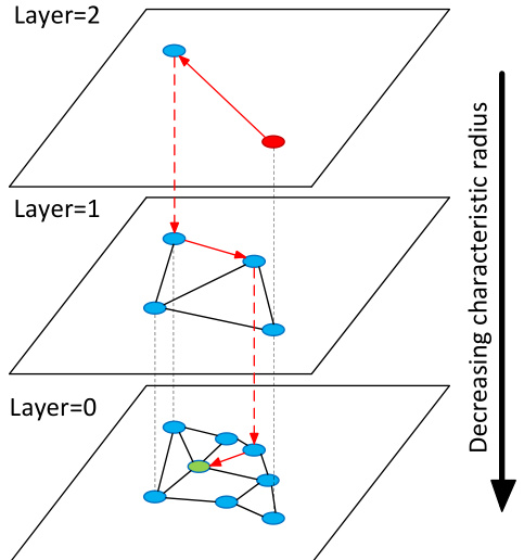
Fig. 1. Illustration of the Hierarchical NSW idea. The search starts from an element from the top layer (shown red). Red arrows show direction of the greedy algorithm from the entry point to the query (shown green).
图 1: 分层 NSW (Navigable Small World) 算法示意图。搜索从顶层元素(红色显示)开始。红色箭头显示贪婪算法从入口点到查询点(绿色显示)的搜索路径。
One way to form such a layered structure is to explicitly set links with different length scales by introducing layers. For every element we select an integer level $I$ which defines the maximum layer for which the element belongs to. For all elements in a layer a proximity graph (i.e. graph containing only “short” links that approximate Delaunay graph) is built increment ally. If we set an exponentially decaying probability of $I$ (i.e. following a geometric distribution) we get a logarithmic scaling of the expected number of layers in the structure. The search procedure is an iterative greedy search starting from the top layer and finishing at the zero layer.
构建这种分层结构的一种方法是通过引入层级来显式设置不同长度尺度的链接。为每个元素选定一个整数层级$I$,该值定义了元素所属的最高层级。系统会逐层为每层中的所有元素增量构建邻近图(即仅包含近似Delaunay图的"短"链接的图)。若设定$I$呈指数衰减概率(即遵循几何分布),则可实现结构中预期层数的对数级缩放。搜索过程采用迭代贪婪算法,从顶层开始搜索直至第零层结束。
In case we merge connections from all layers, the structure becomes similar to the NSW graph (in this case the $I$ can be put in correspondence to the node degree in NSW). In contrast to NSW, Hierarchical NSW construction algorithm does not require the elements to be shuf- fled before the insertion - the stochastic it y is achieved by using level random iz ation, thus allowing truly incremental indexing even in case of temporarily alterating data distribution (though changing the order of the insertion slightly alters the performace due to only partially determen is tic construction procedure).
如果我们将所有层的连接合并,结构会变得类似于NSW图(此时$I$可以与NSW中的节点度对应)。与NSW不同,分层NSW构建算法在插入前不需要对元素进行洗牌——其随机性通过层级随机化实现,从而即使在数据分布暂时变化的情况下也能实现真正的增量索引(尽管由于构建过程仅部分确定性,插入顺序的轻微变化会略微影响性能)。
The Hierarchical NSW idea is also very similar to a well-known 1D probabilistic skip list structure [27] and can be described using its terms. The major difference to skip list is that we generalize the structure by replacing the linked list with proximity graphs. The Hierarchical
分层NSW的想法也与著名的1D概率跳表结构[27]非常相似,可以用其术语描述。与跳表的主要区别在于,我们通过用邻近图替换链表来泛化该结构。分层
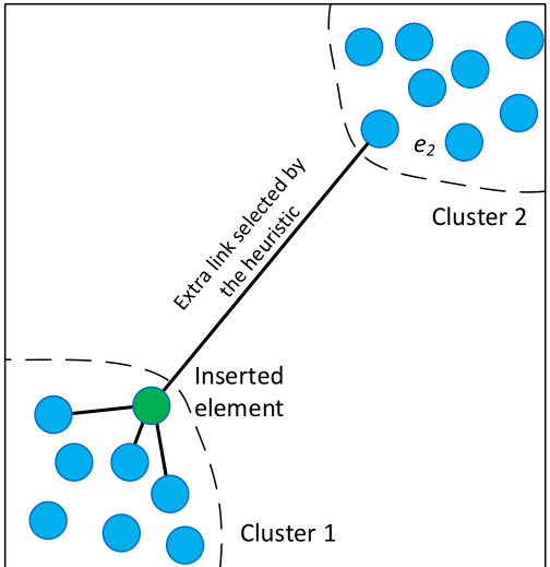
Fig. 2. Illustration of the heuristic used to select the graph neighbors for two isolated clusters. A new element is inserted on the boundary of Cluster 1. All of the closest neighbors of the element belong to the Cluster 1, thus missing the edges of Delaunay graph between the clusters. The heuristic, however, selects element $\scriptstyle{e_{2}}$ from Cluster 2, thus, maintaining the global connectivity in case the inserted element is the closest to $\boldsymbol{e}_{2}$ compared to any other element from Cluster 1.
图 2: 用于为两个孤立集群选择图邻接点的启发式方法示意图。一个新元素被插入到集群1的边界上。该元素的所有最近邻都属于集群1,因此遗漏了集群间Delaunay图的边。然而,该启发式方法会从集群2中选择元素$\scriptstyle{e_{2}}$,从而在插入元素比集群1中任何其他元素更接近$\boldsymbol{e}_{2}$时保持全局连通性。
NSW approach thus can utilize the same methods for making the distributed approximate search/overlay structures [45].
因此,NSW方法可以利用相同的方法来构建分布式近似搜索/覆盖结构[45]。
For the selection of the proximity graph connections during the element insertion we utilize a heuristic that takes into account the distances between the candidate elements to create diverse connections (a similar algorithm was utilized in the spatial approximation tree [4] to select the tree children) instead of just selecting the closest neighbors. The heuristic examines the candidates starting from the nearest (with respect to the inserted element) and creates a connection to a candidate only if it is closer to the base (inserted) element compared to any of the already connected candidates (see Section 4 for the details).
在元素插入过程中选择邻近图连接时,我们采用了一种启发式方法,该方法不仅考虑候选元素之间的距离来创建多样化连接(空间近似树[4]中采用了类似算法来选择子树节点),而非仅选择最近邻。该启发式方法从距离插入元素最近的候选元素开始检查,仅当候选元素比已连接的任何候选元素更接近基准(插入)元素时,才建立连接(详见第4节)。
When the number of candidates is large enough the heuristic allows getting the exact relative neighborhood graph [46] as a subgraph, a minimal subgraph of the Delaunay graph deducible by using only the distances between the nodes. The relative neighborhood graph allows easily keeping the global connected component, even in case of highly clustered data (see Fig. 2 for illustration). Note that the heuristic creates extra edges compared to the exact relative neighborhood graphs, allowing controlling the number of the connections which is important for search performance. For the case of 1D data the heuristic allows getting the exact Delaunay subgraph (which in this case coincides with the relative neighborhood graph) by using only information about the distances between the elements, thus making a direct transition from Hierarchical NSW to the 1D probabilistic skip list algorithm.
当候选数量足够大时,该启发式方法能精确获取相对邻域图 [46] 作为子图,这是仅通过节点间距即可推导出的Delaunay图最小子图。即使面对高度聚集的数据,相对邻域图也能轻松保持全局连通分量(图示见图 2)。需注意,相比精确的相对邻域图,该启发式方法会生成额外边,从而可调控连接数量——这对搜索性能至关重要。在一维数据场景中,该启发式方法仅需元素间距信息即可获得精确的Delaunay子图(此时与相对邻域图重合),由此实现了从分层NSW到一维概率跳跃表算法的直接过渡。
Base variant of the Hierarchical NSW proximity graphs was also used in ref. [18] (called ‘sparse neighborhood graphs’) for proximity graph searching. Similar heuristic was also a focus of the FANNG algorithm [47]
分层NSW邻近图的基础变体也被文献[18](称为"稀疏邻域图")用于邻近图搜索。类似的启发式方法也是FANNG算法[47]的研究重点。
Algorithm 1
算法 1
(published shortly after the first versions of the current manuscript were posted online) with a slightly different interpretation, based on the sparse neighborhood graph’s property of the exact routing [18].
(在当前稿件初版上线后不久发表)基于稀疏邻域图的精确路由特性[18],提出了略有不同的解读方案。
4 ALGORITHM DESCRIPTION
4 算法描述
Network construction algorithm (alg. 1) is organized via consecutive insertions of the stored elements into the graph structure. For every inserted element an integer maximum layer $I$ is randomly selected with an exponentially decaying probability distribution (normalized by the $m_{L}$ parameter, see line 4 in alg. 1).
网络构建算法(alg. 1)通过将存储元素连续插入图结构来组织。对于每个插入的元素,会按照指数衰减的概率分布(由参数$m_{L}$归一化,参见alg. 1第4行)随机选择一个整数最大层$I$。
The first phase of the insertion process starts from the top layer by greedily traversing the graph in order to find the ef closest neighbors to the inserted element $q$ in the layer. After that, the algorithm continues the search from the next layer using the found closest neighbors from the previous layer as enter points, and the process repeats. Closest neighbors at each layer are found by a variant of the greedy search algorithm described in alg. 2, which is an updated version of the algorithm from [26]. To obtain the approximate $e f$ nearest neighbors in some layer $I_{c},$ a dynamic list $W$ of $e f$ closest found elements (initially filled with enter points) is kept during the search. The list is updated at each step by evaluating the neighborhood of the closest previously non-evaluated element in the list until the neighborhood of every element from the list is evaluated. Compared to limiting the number of distance calculations, Hierarchical NSW stop condition has an advantage - it allows discarding candidates for evalution that are further from the query than the furthest element in the list, thus avoiding bloating of search structures. As in NSW, the list is emulated via two priority queues for better performance. The distinctions from NSW (along with some queue optimization s) are: 1) the enter point is a fixed parameter; 2) instead of changing the number of multi-searches, the quality of the search is controlled by a different parameter $e f$ (which was set to $K$ in NSW [26]).
插入过程的第一阶段从顶层开始,通过贪婪遍历图来寻找当前层中与插入元素$q$最接近的$ef$个邻居。随后,算法以前一层找到的最近邻作为入口点,在下一层继续搜索,该过程循环执行。每层最近邻的查找采用算法2描述的贪婪搜索变体实现,这是对文献[26]算法的改进版本。
为获取某层$I_c$中的近似$ef$最近邻,搜索过程中会动态维护一个包含$ef$个最近元素的列表$W$(初始值为入口点)。该列表通过逐步评估列表中最近未探索元素的邻域进行更新,直到列表中所有元素的邻域都被评估完毕。相比限制距离计算次数的方案,分层NSW的终止条件具有优势——它能排除比列表中最远元素距离查询点更远的候选对象,从而避免搜索结构膨胀。与NSW类似,该列表通过双优先队列模拟以获得更好性能。其与NSW的区别(包括队列优化)在于:1) 入口点为固定参数;2) 通过独立参数$ef$(NSW[26]中设为$K$)而非改变多重搜索次数来控制搜索质量。
Algorithm 2
算法 2
SEARCH-LAYER(q, ep, ef, lc)
SEARCH-LAYER(q, ep, ef, lc)
Algorithm 5
算法 5
During the first phase of the search the ef parameter is set to 1 (simple greedy search) to avoid introduction of additional parameters.
在搜索的第一阶段,ef参数设为1(简单贪心搜索)以避免引入额外参数。
When the search reaches the layer that is equal or less than $l,$ the second phase of the construction algorithm is initiated. The second phase differs in two points: 1) the $e f$ parameter is increased from 1 to ef Construction in order to control the recall of the greedy search procedure; 2) the found closest neighbors on each layer are also used as candidates for the connections of the inserted element.
当搜索到达小于或等于 $l$ 的层级时,构建算法的第二阶段启动。第二阶段有两点不同:1) 将 $ef$ 参数从1增加到 ef Construction,以控制贪心搜索过程的召回率;2) 在每一层找到的最近邻也被用作插入元素的连接候选。
Two methods for the selection of $M$ neighbors from the candidates were considered: simple connection to the closest elements (alg. 3) and the heuristic that accounts for the distances between the candidate elements to create connections in diverse directions (alg. 4), described in the Section 3. The heuristic has two additional parameters: extend Candidates (set to false by default) which extends the candidate set and useful only for extremely clustered data, and keep Pruned Connections which allows getting fixed number of connection per element. The maximum number of connections that an element can have per layer is defined by the parameter $M_{m a x}$ for every layer higher than zero (a special parameter $M_{m a x\theta}$ is used for the ground layer separately). If a node is already full at the moment of making of a new connection, then its extended connection list gets shrunk by the same algorithm that used for the neighbors selection (algs. 3 or 4).
从候选元素中选择 $M$ 个邻居的两种方法被考虑:简单连接最近元素(算法3)和考虑候选元素间距离以创建多样化方向连接的启发式方法(算法4),详见第3节。该启发式方法有两个额外参数:extendCandidates(默认设为false)用于扩展候选集(仅对极端聚集数据有效),以及keepPrunedConnections用于确保每个元素获得固定数量的连接。对于高于零的每一层,元素每层最大连接数由参数 $M_{max}$ 定义(地面层单独使用特殊参数 $M_{max\theta}$)。若节点在新连接建立时已达上限,则其扩展连接列表会通过邻居选择相同算法(算法3或4)进行缩减。
The insertion procedure terminates when the connections of the inserted elements are established on the zero layer.
当插入元素的连接在第零层建立时,插入过程终止。
The K-ANNS search algorithm used in Hierarchical NSW is presented in alg. 5. It is roughly equivalent to the insertion algorithm for an item with layer $_{I=0}$ . The difference is that the closest neighbors found at the ground layer which are used as candidates for the connections are now returned as the search result. The quality of the search is controlled by the $e f$ parameter (corresponding to ef Construction in the construction algorithm).
分层NSW中使用的K-ANNS搜索算法如算法5所示。该算法基本等同于层数为$_{I=0}$时的元素插入算法,区别在于:原先作为连接候选的底层最近邻集合,现在将作为搜索结果返回。搜索质量由$e f$参数控制(对应构建算法中的ef Construction参数)。
4.1 Influence of the construction parameters
4.1 施工参数的影响
Algorithm construction parameters $m_{L}$ and $M_{m a x O}$ are responsible for maintaining the small world navigability in the constructed graphs. Setting $m_{L}$ to zero (this corresponds to a single layer in the graph) and $M_{m a x O}$ to $M$ leads to production of directed $\mathrm{k}$ -NN graphs with a power-law search complexity well studied before [21, 29] (assuming using the alg. 3 for neighbor selection). Setting $m_{L}$ to zero and $M_{m a x\theta}$ to infinity leads to production of NSW graphs with poly logarithmic complexity [25, 26]. Finally, setting $m_{L}$ to some non-zero value leads to emergence of controllable hierarchy graphs which allow logarithmic search complexity by introduction of layers (see the Section 3).
算法构建参数 $m_{L}$ 和 $M_{maxO}$ 负责维持所构建图结构的小世界可导航性。将 $m_{L}$ 设为零(对应图中单层结构)且 $M_{maxO}$ 设为 $M$ 时,会生成具有幂律搜索复杂度的有向k近邻图(directed k-NN graphs),该特性在先前研究中已被充分论证 [21, 29](假设使用算法3进行邻居选择)。当 $m_{L}$ 设为零且 $M_{maxθ}$ 设为无穷大时,将生成具有多重对数复杂度的NSW图 [25, 26]。最后,将 $m_{L}$ 设为非零值时,会产生可控层级图结构,通过引入层级实现对数级搜索复杂度(参见第3节)。
To achieve the optimum performance advantage of the controllable hierarchy, the overlap between neighbors on different layers (i.e. percent of element neighbors that are also belong to other layers) has to be small. In order to decrease the overlap we need to decrease the $m_{L}$ . However, at the same time, decreasing $m_{L}$ leads to an increase of average hop number during a greedy search on each layer, which negatively affects the performance. This leads to existence of the optimal value for the $m_{L}$ parameter.
为实现可控层级结构的最佳性能优势,不同层级间邻居的重叠度(即元素邻居同时属于其他层级的比例)必须尽可能小。为降低重叠度,需要减小参数 $m_{L}$ 。然而,这会同时导致各层贪婪搜索的平均跳数增加,从而对性能产生负面影响。因此,参数 $m_{L}$ 存在一个最优值。
A simple choice for the optimal $m_{L}$ is $1/\ln(M),$ this corresponds to the skip list parameter $_ {p=1/M}$ with an average single element overlap between the layers. Simulations done on an Intel Core i7 5930K CPU show that the proposed selection of $m_{L}$ is a reasonable choice (see Fig. 3 for data on 10M random ${\mathrm{d}}{=}4$ vectors). In addition, the plot demonstrates a massive speedup on low dimensional data when increasing the $m_{L}$ from zero and the effect of using the heuristic for selection of the graph connections. It is hard to expect the same behavior for high dimensional data since in this case the $\mathbf{k}$ -NN graph already has very short greedy algorithm paths [28]. Surprisingly, increasing the $m_{L}$ from zero leads to a measurable increase in speed on very high dimensional data (100k dense random ${\mathrm{d}}{=}1024$ vectors, see plot in Fig. 4), and does not introduce any penalty for the Hierarchical NSW approach. For real data such as SIFT vectors [1] (which have complex mixed structure), the performance improvement by increasing the $m_{L}$ is higher, but less prominent at current settings compared to improvement from the heuristic (see Fig. 5 for 1-NN search performance on 5 million 128- dimensional SIFT vectors from the learning set of BIGANN [13]).
最优 $m_{L}$ 的一个简单选择是 $1/\ln(M)$,这对应于跳跃列表参数 $_ {p=1/M}$,各层之间平均单元素重叠。在 Intel Core i7 5930K CPU 上进行的仿真表明,所提出的 $m_{L}$ 选择是合理的(关于 1000 万个随机 ${\mathrm{d}}{=}4$ 向量的数据见图 3)。此外,该图展示了在低维数据上,当 $m_{L}$ 从零开始增加时带来的显著加速效果,以及使用启发式方法选择图连接的效果。对于高维数据,很难预期相同的行为,因为在这种情况下 $\mathbf{k}$-NN 图已经具有非常短的贪心算法路径 [28]。令人惊讶的是,在极高维数据(10 万个密集随机 ${\mathrm{d}}{=}1024$ 向量,见图 4)上,将 $m_{L}$ 从零开始增加仍能带来可测量的速度提升,且不会对分层 NSW 方法引入任何惩罚。对于 SIFT 向量 [1] 等真实数据(具有复杂的混合结构),增加 $m_{L}$ 带来的性能提升更高,但在当前设置下相比启发式方法的改进效果不那么显著(关于 BIGANN [13] 学习集中 500 万个 128 维 SIFT 向量的 1-NN 搜索性能见图 5)。
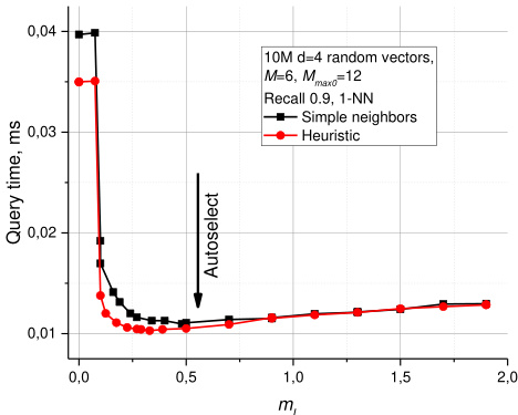
Fig. 3. Plots for query time vs $m_{L}$ parameter for 10M random vectors with ${\mathsf{d}}{=}4$ . The autoselected value $1/\ln(M)$ for $m_{L}$ is shown by an arrow.
图 3: 针对维度 ${\mathsf{d}}{=}4$ 的1000万随机向量,查询时间与参数 $m_{L}$ 的关系图。箭头标示了自动选择的 $m_{L}$ 值 $1/\ln(M)$。
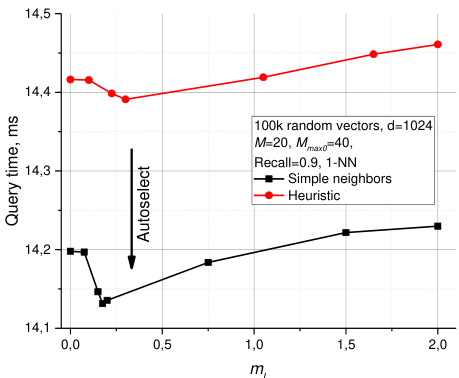
Fig. 4. Plots for query time vs $m_{L}$ parameter for $100k$ random vectors with ${\mathsf{d}}{=}1024$ . The auto selected value $1/\mathsf{I n}(M)$ for $m_{L}$ is shown by an arrow.
图 4: 查询时间与参数 $m_{L}$ 的关系图,基于 $100k$ 个随机向量 (${\mathsf{d}}{=}1024$) 。箭头标示了自动选择的 $m_{L}$ 值 $1/\mathsf{I n}(M)$ 。
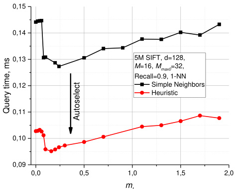
Fig. 5. Plots for query time vs $m_{L}$ parameter for 5M SIFT learn dataset. The auto selected value $1/\mathsf{I n}(M)$ for $m_{L}$ is shown by an arrow.
图 5: 针对500万SIFT学习数据集的查询时间与参数$m_{L}$的关系图。箭头标示了$m_{L}$的自动选择值$1/\mathsf{In}(M)$。
Selection of the $M_{m a x\theta}$ (the maximum number of connections that an element can have in the zero layer) also has a strong influence on the search performance, especially in case of high quality (high recall) search. Simulations show that setting $M_{m a x\theta}$ to $M$ (this corresponds to kNN graphs on each layer if the neighbors selection heuristic is not used) leads to a very strong performance penalty at high recall. Simulations also suggest that $2{\cdot}M$ is a good choice for $M_{m a x\dot{\rho}}$ setting the parameter higher leads to performance degradation and excessive memory usage. In Fig. 6 there are presented results of search performance for the 5M SIFT learn dataset depending on the $M_{m a x\theta}$ parameter (done on an Intel Core i5 2400 CPU). The suggested value gives performance close to optimal at different recalls.
$M_{max\theta}$ (元素在零层可拥有的最大连接数) 的选择对搜索性能有显著影响,特别是在高质量(高召回率)搜索场景下。仿真实验表明,将 $M_{max\theta}$ 设为 $M$ (若不使用邻居选择启发式算法,则相当于每层构建kNN图)会导致高召回率时性能急剧下降。实验数据同时表明,$2{\cdot}M$ 是 $M_{max\rho}$ 的理想取值,过高参数设置会引起性能衰退和内存占用激增。图6展示了基于5M SIFT学习数据集的搜索性能随 $M_{max\theta}$ 参数变化的测试结果(实验平台为Intel Core i5 2400 CPU),该推荐值能在不同召回率下保持接近最优的性能表现。
In all of the considered cases, use of the heuristic for proximity graph neighbors selection (alg. 4) leads to a higher or similar search performance compared to the naïve connection to the nearest neighbors (alg. 3). The effect is the most prominent for low dimensional data, at high recall for mid-dimensional data and for the case of highly clustered data (ideologically discontinuity can be regarded as a local low dimensional feature), see the comparison in Fig. 7 (Core i5 2400 CPU). When using the closest neighbors as connections for the proximity graph, the Hierarchical NSW algorithm fails to achieve a high recall for clustered data because the search stucks at the clusters boundaries. Contrary, when the heuristic is used (together with candidates’ extension, line 3 in Alg. 4), clustering leads to even higher performance. For uniform and very high dimensional data there is a little difference between the neighbors selecting methods (see Fig. 4), possibly due to the fact that in this case almost all of the nearest neighbors are selected by the heuristic.
在所有考虑的情况下,使用启发式方法选择邻近图邻居(算法4)相比直接连接最近邻的朴素方法(算法3),能带来更高或相似的搜索性能。这一效果在低维数据中最为显著,在中维数据的高召回率场景以及高度聚类的数据中(理论上不连续性可视为局部低维特征)也表现突出,具体对比见图7(Core i5 2400 CPU)。当采用最近邻作为邻近图的连接方式时,分层NSW算法在聚类数据上难以实现高召回率,因为搜索会卡在聚类边界。相反,当使用启发式方法(结合候选扩展,算法4第3行)时,聚类反而会带来更高的性能。对于均匀分布和极高维数据,邻居选择方法之间的差异较小(见图4),这可能是因为在此情况下几乎所有最近邻都会被启发式方法选中。
The only meaningful construction parameter left for the user is $M.$ A reasonable range of $M$ is from 5 to 48. Simulations show that smaller $M$ generally produces better results for lower recalls and/or lower dimensional data, while bigger $M$ is better for high recall and/or high dimensional data (see Fig. 8 for illustration, Core i5 2400 CPU). The parameter also defines the memory consumption of the algorithm (which is proportional to $M)$ , so it should be selected with care.
用户唯一需要设置的有意义的构造参数是 $M$。$M$ 的合理取值范围为 5 至 48。模拟实验表明:较小的 $M$ 通常在低召回率和/或低维数据场景下表现更优,而较大的 $M$ 更适合高召回率和/或高维数据场景 (具体示例见图 8,测试平台为 Core i5 2400 CPU)。该参数同时决定了算法的内存占用量 (与 $M$ 成正比),因此需谨慎选择。
Selection of the ef Construction parameter is straight forward. As it was suggested in [26] it has to be large enough to produce K-ANNS recall close to unity during the construction process (0.95 is enough for the most usecases). And just like in [26], this parameter can possibly be auto-configured by using sample data.
选择ef构造参数的方法很直接。如[26]中所述,该参数需要足够大,以在构建过程中使K-ANNS召回率接近1(大多数应用场景下0.95即可)。与[26]类似,此参数也可以通过采样数据自动配置。
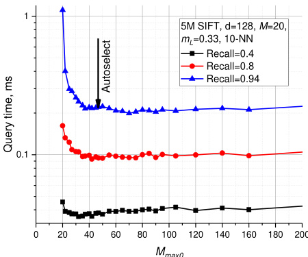
Fig. 6. Plots for query time vs $M_{m a x O}$ parameter for 5M SIFT learn dataset. The auto selected value $_ {2\cdot M}$ for $M_{m a x O}$ is shown by an arrow.
图 6: 针对5M SIFT学习数据集的查询时间与$M_{maxO}$参数的对比图。箭头标示了自动选择的$_ {2\cdot M}$作为$M_{maxO}$的值。
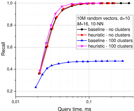
Fig. 7. Effect of the method of neighbor selections (baseline corresponds to alg. 3, heuristic to alg. 4) on clustered (100 random isolated clusters) and non-clustered ${\mathsf{d}}{=}10$ random vector data.
图 7: 邻居选择方法对聚类(100个随机孤立簇)和非聚类 ${\mathsf{d}}{=}10$ 随机向量数据的影响(基线对应算法3,启发式对应算法4)。
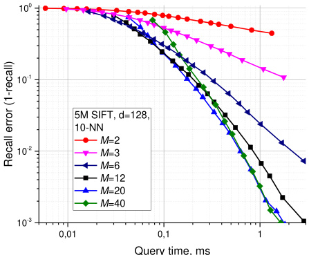
Fig. 8. Plots for recall error vs query time for different parameters of $M$ for Hierarchical NSW on 5M SIFT learn dataset.
图 8: 在500万SIFT学习数据集上,Hierarchical NSW算法针对不同参数M的召回错误率与查询时间关系图。
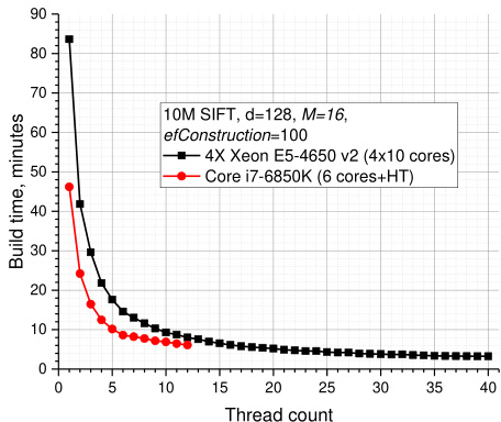
Fig. 9. Construction time for Hierarchical NSW on 10M SIFT dataset for different numbers of threads on two CPUs.
图 9: 两种CPU上不同线程数对10M SIFT数据集构建Hierarchical NSW索引的时间对比
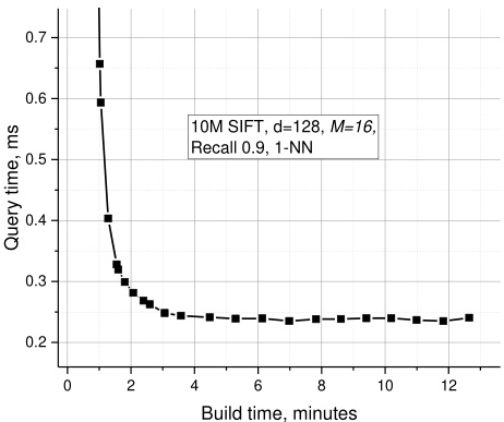
Fig. 10. Plots of the query time vs construction time tradeoff for Hierarchical NSW on 10M SIFT dataset.
图 10: 在1000万SIFT数据集上Hierarchical NSW的查询时间与构建时间权衡关系图

Fig. 11. Plots of the ef parameter required to get fixed accuracies vs the dataset size for ${\mathsf{d}}{=}4$ random vector data.
图 11: 在维度 ${\mathsf{d}}{=}4$ 的随机向量数据中,为达到固定准确率所需的 ef 参数随数据集大小的变化曲线。
The construction process can be easily and efficiently parallel i zed with only few synchronization points (as demonstrated in Fig. 9) and no measurable effect on index quality. Construction speed/index quality tradeoff is controlled via the ef Construction parameter. The tradeoff between the search time and the index construction time is presented in Fig. 10 for a 10M SIFT dataset and shows that a reasonable quality index can be constructed for ef Construction $\scriptstyle=100$ on a 4X 2.4 GHz 10-core Xeon E5- 4650 v2 CPU server in just 3 minutes. Further increase of the ef Construction leads to little extra performance but in exchange of significantly longer construction time.
构建过程可以轻松高效地并行化,仅需少量同步点(如图 9 所示)且对索引质量无显著影响。构建速度与索引质量的权衡通过 efConstruction 参数控制。图 10 展示了 10M SIFT 数据集上的搜索时间与索引构建时间的权衡关系:在 4X 2.4 GHz 10 核 Xeon E5-4650 v2 CPU 服务器上,仅需 3 分钟即可为 efConstruction $\scriptstyle=100$ 构建出质量合理的索引。继续增大 efConstruction 参数虽能带来微小的性能提升,但会显著增加构建时间。
4.2 Complexity analysis
4.2 复杂度分析
4.2.1 Search complexity
4.2.1 搜索复杂度
The complexity scaling of a single search can be strictly analyzed under the assumption that we build exact Delaunay graphs instead of the approximate ones. Suppose we have found the closest element on some layer (this is guaranteed by having the Delaunay graph) and then descended to the next layer. One can show that the average number of steps before we find the closest element in the layer is bounded by a constant.
在假设我们构建的是精确Delaunay图而非近似图的前提下,可以严格分析单次搜索的复杂度缩放。假设我们在某层已找到最近邻元素(由Delaunay图的性质保证)并下降到下一层,可以证明:在该层中找到最近邻元素的平均步骤数存在常数上界。
Indeed, the layers are not correlated with the spatial positions of the data elements and, thus, when we traverse the graph there is a fixed probability $p{=}\mathrm{exp}({\cdot}m_{L})$ that the next node belongs to the upper layer. However, the search on the layer always terminates before it reaches the element which belongs to the higher layer (otherwise the search on the upper layer would have stopped on a different element), so the probability of not reaching the target on s-th step is bounded by $\exp(-s\cdot m_{L}).$ Thus the expected number of steps in a layer is bounded by a sum of geometric progression $S\mathrm{=}1/(1\mathrm{-exp}(\mathrm{-}m_{L})),$ which is independent of the dataset size.
事实上,各层与数据元素的空间位置并无关联,因此当我们遍历图时,下一个节点属于上层的固定概率为 $p{=}\mathrm{exp}({\cdot}m_{L})$。然而,层上的搜索总会在到达属于更高层的元素前终止(否则上层搜索本应在另一元素处停止),因此未能在第s步到达目标的概率上限为 $\exp(-s\cdot m_{L})$。故而层内预期步数上限为几何级数之和 $S\mathrm{=}1/(1\mathrm{-exp}(\mathrm{-}m_{L}))$,该值与数据集规模无关。
If we assume that the average degree of a node in the Delaunay graph is capped by a constant $C$ in the limit of the large dataset (this is the case for random Euclid data [48], but can be in principle violated in exotic spaces), then the overall average number of distance evaluations in a layer is bounded by a constant $C\cdot S,$ independently of the dataset size.
如果我们假设在大数据集的极限情况下,Delaunay图中节点的平均度数被常数$C$限制(随机欧几里得数据[48]即属此情况,但在特殊空间中可能不成立),那么每一层的平均距离计算次数将被常数$C\cdot S$限制,与数据集规模无关。
And since the expectation of the maximum layer index by the construction scales as $\mathrm{O}(\log(N))$ , the overall complexity scaling is ${\mathrm{O}}(\log(N)),$ in agreement with the simulations on low dimensional datasets.
由于最大层索引的期望值按构造规模为 $\mathrm{O}(\log(N))$ ,整体复杂度规模为 ${\mathrm{O}}(\log(N))$ ,这与低维数据集的模拟结果一致。
The inital assumption of having the exact Delaunay graph violates in Hierarchical NSW due to usage of approximate edge selection heuristic with a fixed number of neighbors per element. Thus, to avoid stucking into a local minimum the greedy search algorithm employs a backtracking procedure on the zero layer. Simulations show that at least for low dimensional data (Fig. 11, $\mathrm{d}{=}4$ ) the dependence of the required ef parameter (which determines the complexity via the minimal number of hops during the backtracking) to get a fixed recall saturates with the rise of the dataset size. The backtracking complexity is an additive term in respect to the final complexity, thus, as follows from the empirical data, inaccuracies of the Delaunay graph approximation do not alter the scaling.
由于在分层NSW中使用了固定邻居数量的近似边选择启发式方法,最初假设的精确Delaunay图不再成立。因此,为避免陷入局部最小值,贪婪搜索算法在零层采用了回溯过程。模拟显示,至少在低维数据中(图11:$\mathrm{d}{=}4$),为达到固定召回率所需的ef参数(通过回溯过程中的最小跳数决定复杂度)随数据集规模增大会趋于饱和。回溯复杂度相对于最终复杂度是一个加性项,因此根据实验数据,Delaunay图近似的误差不会改变缩放规律。
Such empirical investigation of the Delaunay graph approximation resilience requires having the average number of Delaunay graph edges independent of the dataset to evidence how well the edges are approximated with a constant number of connections in Hierarchical NSW. However, the average degree of Delaunay graph scales exponentially with the dimensionality [39]), thus for high dimensional data (e.g. $\mathsf{d}{=}128$ ) the aforementioned condition requires having extremely large datasets, making such empricial investigation unfeasible. Further analitical evidence is required to confirm whether the resilience of Delaunay graph a proxima t ions generalizes to higher dimensional spaces.
对Delaunay图近似鲁棒性的实证研究需要确保Delaunay图边的平均数量与数据集无关,以证明在Hierarchical NSW中使用恒定连接数对边的近似效果。然而,Delaunay图的平均度随维度呈指数级增长 [39],因此对于高维数据(例如 $\mathsf{d}{=}128$),上述条件需要极大尺寸的数据集,使得此类实证研究难以实现。需进一步的理论分析来验证Delaunay图近似的鲁棒性是否适用于更高维空间。
4.2.2 Construction complexity
4.2.2 构建复杂度
The construction is done by iterative insertions of all elements, while the insertion of an element is merely a sequence of K-ANN-searches at different layers with a subsequent use of heuristic (which has fixed complexity at fixed ef Construction). The average number of layers for an element to be added in is a constant that depends on $m_{L}$ :
构建过程是通过迭代插入所有元素完成的,而插入一个元素仅需在不同层执行一系列K-ANN搜索,随后应用启发式方法(在固定ef Construction参数下具有固定复杂度)。元素被插入的平均层数是一个取决于 $m_{L}$ 的常数:
$$
E\big[l+1\big]=E\big[-\ln(u n i f(0,1))\bullet m_{L}\big]+1=m_{L}+1
$$
$$
E\big[l+1\big]=E\big[-\ln(u n i f(0,1))\bullet m_{L}\big]+1=m_{L}+1
$$
Thus, the insertion complexiy scaling is the same as the one for the search, meaning that at least for relatively low dimensional datasets the construction time scales as $\mathrm{O}(N{\cdot}\mathrm{log}(N))$ .
因此,插入操作的复杂度扩展与搜索操作相同,这意味着至少在维度相对较低的数据集中,构建时间按 $\mathrm{O}(N{\cdot}\mathrm{log}(N))$ 比例增长。
4.2.3 Memory cost
4.2.3 内存成本
The memory consumption of the Hierarchical NSW is mostly defined by the storage of graph connections. The number of connections per element is $M_{m a x\theta}$ for the zero layer and $M_{m a x}$ for all other layers. Thus, the average memory consumption per element is $(M_{m a x}\partial^{+}m_{L}\cdot M_{m a x})$ ∙bytes per link. If we limit the maximum total number of elements by approximately four billions, we can use four-byte unsigned integers to store the connections. Tests suggest that typical close to optimal $M$ values usually lie in a range between 6 and 48. This means that the typical memory requirements for the index (excluding the size of the data) are about 60-450 bytes per object, which is in a good agreement with the simulations.
分层NSW的内存消耗主要由图连接的存储决定。每元素的连接数在零层为$M_{max\theta}$,其他所有层为$M_{max}$。因此,平均每个元素的内存消耗为$(M_{max}\partial^{+}m_{L}\cdot M_{max})$∙每链接字节数。若将元素总数上限设为约40亿,可使用4字节无符号整数存储连接。测试表明,接近最优的$M$值通常介于6到48之间。这意味着索引的典型内存需求(不包括数据大小)约为每个对象60-450字节,与模拟结果高度吻合。
5 PERFORMANCE EVALUATION
5 性能评估
The Hierarchical NSW algorithm was implemented in $\mathsf{C}\mathsf{+}\mathsf{+}$ on top of the Non Metric Space Library (nmslib) $[49]^{1}.$ , which already had a functional NSW imple ment ation (under name “sw-graph”). Due to several limitations posed by the library, to achieve a better performance, the Hierarchical NSW implementation uses custom distance functions together with C-style memory management, which avoids unnecessary implicit addressing and allows efficient hardware and software prefetching during the graph traversal.
分层NSW算法基于非度量空间库(nmslib) [49]¹在$\mathsf{C}\mathsf{+}\mathsf{+}$中实现。该库已具备基础NSW实现(命名为"sw-graph")。由于库本身的若干限制,为实现更优性能,分层NSW实现采用了自定义距离函数与C风格内存管理,这种组合既避免了不必要的隐式寻址,又能在图遍历过程中实现高效的软硬件预取。
Comparing the performance of K-ANNS algorithms is a nontrivial task since the state-of-the-art is constantly changing as new algorithms and implementations are emerging. In this work we concentrated on comparison with the best algorithms in Euclid spaces that have open source implementations. An implementation of the Hierarchical NSW algorithm presented in this paper is also distributed as a part of the open source nmslib library1 together with an external $\mathsf{C}\mathsf{+}\mathsf{+}$ memory-efficient headeronly version with support for incremental index construction2.
比较K-ANNS算法的性能并非易事,因为随着新算法和实现的不断涌现,当前最优技术也在持续更新。本研究中,我们主要聚焦于与欧几里得空间中具有开源实现的最佳算法进行对比。本文提出的分层NSW算法实现已作为开源nmslib库1的一部分发布,同时提供了一个外部$\mathsf{C}\mathsf{+}\mathsf{+}$内存高效头文件版本2,支持增量索引构建。
The comparison section consists of four parts: comparison to the baseline NSW (5.1), comparison to the state-ofthe-art algorithms in Euclid spaces (5.2), rerun of the subset of tests [34] in general metric spaces in which NSW failed (5.3) and comparison to state-of-the-art PQalgorithms on a large 200M SIFT dataset (5.4).
对比部分包含四个部分:与基线NSW的对比(5.1)、与欧几里得空间中最先进算法的对比(5.2)、在通用度量空间中重新运行NSW失败的测试子集34、以及在200M规模SIFT数据集上与最先进PQ算法的对比(5.4)。
5.1 Comparison with baseline NSW
5.1 与基线NSW的对比
For the baseline NSW algorithm implementation, we used the “sw-graph” from nmslib 1.1 (which is slightly updated compared to the implementation tested in [33, 34]) to demonstrate the improvements in speed and algorithmic complexity (measured by the number of distance computations).
对于基线NSW算法的实现,我们使用了nmslib 1.1中的"sw-graph"(相比[33, 34]中测试的实现略有更新)来展示速度和算法复杂度(通过距离计算次数衡量)的改进。
Fig. 12(a) presents a comparison of Hierarchical NSW to the basic NSW algorithm for ${\mathrm{d}}{=}4$ random hypercube data made on a Core i5 2400 CPU (10-NN search). Hierarchical NSW uses much less distance computations during a search on the dataset, especially at high recalls.
图 12(a) 展示了在 Core i5 2400 CPU 上对 ${\mathrm{d}}{=}4$ 随机超立方体数据进行 10-NN 搜索时,分层 NSW (Hierarchical NSW) 与基础 NSW 算法的对比。分层 NSW 在数据集搜索过程中(尤其是高召回率时)所需的距离计算量显著减少。
The scalings of the algorithms on a $ \scriptstyle{\mathrm{d}}=8$ random hypercube dataset for a 10-NN search with a fixed recall of 0.95 are presented in Fig. 12(b). It clearly de most rates that Hierarchical NSW has a complexity scaling for this setting not worse than logarithmic and outperforms NSW at any dataset size. The performance advantage in absolute time (Fig. 12(c)) is even higher due to improved algorithm imple men tai on.
在 $ \scriptstyle{\mathrm{d}}=8$ 随机超立方体数据集上,针对固定召回率 0.95 的 10-NN 搜索算法扩展性如图 12(b) 所示。该结果清晰表明,在此设置下 Hierarchical NSW 的复杂度扩展不差于对数级,且在任何数据集规模下均优于 NSW。由于算法实现的改进,其绝对时间性能优势(图 12(c))更为显著。
5.2 Comparison in Euclid spaces
5.2 欧几里得空间中的比较
The main part of the comparison was carried out on vector datasets with use of the popular K-ANNS benchmark ann-benchmark3 as a testbed. The testing system utilizes python bindings of the algorithms – it con sequentially runs the K-ANN search for one thousand queries (randomly extracted from the initial dataset) with preset algorithm parameters producing an output containing recall and average time of a single search. The considered algorithms are:
对比的主要部分是在向量数据集上进行的,使用了流行的K-ANNS基准测试ann-benchmark3作为测试平台。测试系统利用算法的Python语言绑定——它按顺序运行一千次查询(从初始数据集中随机提取)的K-ANN搜索,预设算法参数后输出包含召回率和单次搜索平均时间的结果。涉及的算法包括:

Fig. 12. Comparison between NSW and Hierarchical NSW: (a) distance calculation number vs accuracy tradeoff for a 10 million 4- dimensional random vectors dataset; (b-c) performance scaling in term s of number of distance calculations (b) and raw query(c) time on a 8-dimensional random vectors dataset.
图 12: NSW与分层NSW对比: (a) 1000万4维随机向量数据集的距离计算次数与准确率权衡; (b-c) 8维随机向量数据集在距离计算次数(b)和原始查询时间(c)方面的性能扩展。
TABLE 1 Parameters of the used datasets on vector spaces benchmark.
| Dataset | Description | Size | d | BF time | Space |
| SIFT | Image feature vectors[13] | 1M | 128 | 94 ms | L2 |
| GloVe | Word embeddings trained on tweets [52] | 1.2M | 100 | 95ms | cosine |
| CoPhIR | MPEG-7 features extracted from the images [53] | 2M | 272 | 370 ms | L2 |
| Random vectors | Random vectors in hypercube | 30M | 4 | 590 ms | L2 |
| DEEP | One million subset of the billion deep image features dataset [14] | 1M | 96 | 60 ms | L2 |
| MNIST | Handwritten digit images [54] | 60k | 784 | 22 ms | L2 |
表 1: 向量空间基准测试所用数据集的参数。
| 数据集 | 描述 | 大小 | d | BF时间 | 空间 |
|---|---|---|---|---|---|
| SIFT | 图像特征向量 [13] | 1M | 128 | 94 ms | L2 |
| GloVe | 基于推文训练的词嵌入 [52] | 1.2M | 100 | 95 ms | cosine |
| CoPhIR | 从图像中提取的MPEG-7特征 [53] | 2M | 272 | 370 ms | L2 |
| Random vectors | 超立方体中的随机向量 | 30M | 4 | 590 ms | L2 |
| DEEP | 十亿深度图像特征数据集的百万子集 [14] | 1M | 96 | 60 ms | L2 |
| MNIST | 手写数字图像 [54] | 60k | 784 | 22 ms | L2 |
based on random projection tree forest.
基于随机投影树森林。
The comparison was done on a 4X Xeon E5-4650 v2 Debian OS system with ${128~\mathrm{Gb}}$ of RAM. For every algorithm we carefully chose the best results at every recall range to evaluate the best possible performance (with initial values from the testbed defaults). All tests were done in a single thread regime. Hierarchical NSW was compiled using the GCC 5.3 with -Ofast optimization flag.
对比实验在一台搭载4颗Xeon E5-4650 v2处理器、${128~\mathrm{Gb}}$内存的Debian系统上进行。针对每种算法,我们在不同召回率区间精选最优结果以评估其理论最佳性能(初始参数采用测试平台默认值)。所有测试均在单线程环境下完成,其中分层NSW算法使用GCC 5.3编译器并启用-Ofast优化标志进行编译。
The parameters and description of the used datasets are outlined in Table 1. For all of the datasets except GloVe we used the $\mathrm{L}_ {2}$ distance. For GloVe we used the cosine similarity which is equivalent to $\mathrm{L}_{2}$ after vector normalization. The brute-force (BF) time is measured by the nmslib library.
表1列出了所用数据集的参数和描述。除GloVe外,所有数据集均使用$\mathrm{L}_ {2}$距离度量。对于GloVe数据集,我们采用余弦相似度度量(经向量归一化后等同于$\mathrm{L}_{2}$距离)。暴力搜索(BF)耗时通过nmslib库测得。
Results for the vector data are presented in Fig. 13. For SIFT, GloVE, DEEP and CoPhIR datasets Hierarchical NSW clearly outperforms the rivals by a large margin. For low dimensional data $(\mathrm{d}{=}4)$ Hierarchical NSW is slightly faster at high recall compared to the Annoy while strongly outperforms the other algorithms.
向量数据的结果如图 13 所示。对于 SIFT、GloVE、DEEP 和 CoPhIR 数据集,Hierarchical NSW 明显以较大优势领先于其他算法。对于低维数据 $(\mathrm{d}{=}4)$,在高召回率下 Hierarchical NSW 略快于 Annoy,同时显著优于其他算法。
TABLE 2. Used datasets for repetition of the Non-Metric data tests subset.
| Dataset | Description | Size | p | BF time | Distance |
| Wiki-sparse | TF-IDF (term frequency-inverse document frequency) vectors (created via GENSIM [58]) | 4M | 105 | 5.9 s | Sparse cosine |
| Wiki-8 | Topic histograms created from sparse TF-IDF vectors of the wiki-sparse dataset (created via GENSIM [58]) | 2M | 8 | Jensen- Shannon (JS) | |
| Wiki-128 | Topic histograms created from sparse TF-IDF vectors of the wiki-sparse dataset (created via GENSIM[58]) | 2M | 128 | 1.17 s | Jensen- Shannon (JS) divergence |
| ImageNet | Signatures extracted from LSVRC-2014 with SQFD (signature quadratic form) distance [59] | 1M | 272 | 18.3 s | SQFD |
| DNA | DNA (deoxyribonucleic acid) dataset sampled from the Human Genome 5[34]. | 1M | 2.4 s | Levenshtein |
表 2: 用于重复非度量数据测试子集的数据集
| 数据集 | 描述 | 大小 | p | BF时间 | 距离 |
|---|---|---|---|---|---|
| Wiki-sparse | TF-IDF (词频-逆文档频率) 向量 (通过 GENSIM [58] 创建) | 4M | 105 | 5.9 s | 稀疏余弦 (Sparse cosine) |
| Wiki-8 | 从 wiki-sparse 数据集的稀疏 TF-IDF 向量生成的主题直方图 (通过 GENSIM [58] 创建) | 2M | 8 | Jensen-Shannon (JS) | |
| Wiki-128 | 从 wiki-sparse 数据集的稀疏 TF-IDF 向量生成的主题直方图 (通过 GENSIM [58] 创建) | 2M | 128 | 1.17 s | Jensen-Shannon (JS) 散度 |
| ImageNet | 从 LSVRC-2014 提取的签名,使用 SQFD (签名二次型) 距离 [59] | 1M | 272 | 18.3 s | SQFD |
| DNA | 从人类基因组 5 [34] 采样的 DNA (脱氧核糖核酸) 数据集 | 1M | 2.4 s | Levenshtein |
5.3 Comparison in general spaces
5.3 一般空间中的比较
A recent comparison of algorithms [34] in general spaces (i.e. non-symmetric or with violation of triangle inequality) showed that the baseline NSW algorithm has severe problems on low dimensional datasets. To test the performance of the Hierarchical NSW algorithm we have repeated a subset of tests from [34] on which NSW performed poorly or suboptimal. For that purpose we used a built-in nmslib testing system which had scripts to run tests from [34]. The evaluated algorithms included the VP-tree, permutation techniques (NAPP and bruteforce filtering) [49, 55-57], the basic NSW algorithm and NNDescent-produced proximity graphs [29] (both in pair with the NSW graph search algorithm). As in the original tests, for every dataset the test includes the results of either NSW or NNDescent, depending on which structure performed better. No custom distance functions or special memory management were used in this case for Hierarchical NSW leading to some performance loss.
最近一项针对通用空间(即非对称或违反三角不等式)算法的比较研究[34]显示,基准NSW算法在低维数据集上存在严重问题。为测试分层NSW算法的性能,我们复现了[34]中NSW表现不佳或次优的部分测试集,使用nmslib内置测试系统运行[34]的测试脚本。评估算法包括VP树、排列技术(NAPP与暴力过滤)[49, 55-57]、基础NSW算法及NNDescent生成的邻近图[29](均与NSW图搜索算法配对使用)。如原始测试所示,每个数据集仅展示NSW或NNDescent中表现更优者的结果。本次测试中分层NSW未使用定制距离函数或特殊内存管理方案,导致部分性能损失。

Fig. 13. Results of the comparison of Hierarchical NSW with open source implementations of K-ANNS algorithms on five datasets for 10- NN searches. The time of a brute-force search is denoted as the BF.
图 13: 在五个数据集上进行的10-NN搜索中,Hierarchical NSW与开源K-ANNS算法实现的对比结果。暴力搜索时间标记为BF。

Fig. 14. Results of the comparison of Hierarchical NSW with general space K-ANNS algorithms from the Non Metric Space Library on five datasets for 10-NN searches. The time of a brute-force search is denoted as the BF.
图 14: 在五个数据集上对分层 NSW 与非度量空间库(Non Metric Space Library)中通用空间 K-ANNS 算法进行 10-NN 搜索的对比结果。暴力搜索时间标记为 BF。
TABLE 3. Parameters for comparison between Hierarchical NSW and Faiss on a 200M subset of 1B SIFT dataset.
| Algorithm | Buildtime | Peak memory (runtime) | Parameters |
| HierarchicalNSW | 5.6hours | 64 Gb | M=16,efConstruction=500 (1) |
| HierarchicalNSW | 42minutes | 64 Gb | M=16,efConstruction=40 (2) |
| Faiss | 12hours | 30 Gb | OPQ64, IMI2x14, PQ64 (1) |
| Faiss | 11hours | 23.5 Gb | OPQ32,IMI2x14, PQ32 (2) |
表 3: 在10亿SIFT数据集的2亿子集上比较Hierarchical NSW和Faiss的参数。
| Algorithm | Buildtime | Peak memory (runtime) | Parameters |
|---|---|---|---|
| HierarchicalNSW | 5.6小时 | 64 GB | M=16, efConstruction=500 (1) |
| HierarchicalNSW | 42分钟 | 64 GB | M=16, efConstruction=40 (2) |
| Faiss | 12小时 | 30 GB | OPQ64, IMI2x14, PQ64 (1) |
| Faiss | 11小时 | 23.5 GB | OPQ32, IMI2x14, PQ32 (2) |
The datasets are summarized in Table 2. Further details of the datasets, spaces and algorithm parameter selection can be found in the original work [34]. The bruteforce (BF) time is measured by the nmslib library.
数据集总结如表 2 所示。关于数据集、空间和算法参数选择的更多细节可以在原始文献 [34] 中找到。暴力搜索 (BF) 时间通过 nmslib 库测量。
The results are presented in Fig. 14. Hierarchical NSW significantly improves the performance of NSW and is a leader for any of the tested datasets. The strongest enhancement over NSW, almost by 3 orders of magnitude is observed for the dataset with the lowest dimensionality, the wiki-8 with JS-divergence. This is an important result that demonstrates the robustness of Hierarchical NSW, as for the original NSW this dataset was a stumbling block. Note that for the wiki-8 to nullify the effect of implementation results are presented for the distance computations number instead of the CPU time.
结果如图14所示。分层NSW显著提升了NSW的性能,在所有测试数据集中均处于领先地位。在维度最低的wiki-8数据集(使用JS散度)上,相比NSW实现了近3个数量级的最大性能提升。这一重要结果证明了分层NSW的鲁棒性,因为对原始NSW而言该数据集曾是性能瓶颈。需注意,针对wiki-8数据集,为消除实现方式的影响,结果展示的是距离计算次数而非CPU时间。
5.4 Comparison with product quantization based algorithms.
5.4 基于乘积量化的算法对比
Product quantization K-ANNS algorithms [10-17] are considered as the state-of-the-art on billion scale datasets since they can efficiently compress stored data, allowing modest RAM usage while achieving millisecond search times on modern CPUs.
乘积量化K-ANNS算法[10-17]被视为十亿级数据集上的最先进技术,因其能高效压缩存储数据,在现代CPU上实现毫秒级搜索的同时保持较低内存占用。
To compare the performance of Hierarchical NSW against PQ algorithms we used the facebook Faiss library8 as the baseline (a new library with state-of-the-art PQ algorithms [12, 15] implementations, released after the current manuscript was submitted) compiled with the OpenBLAS backend. The tests where done for a 200M subset of 1B SIFT dataset [13] on a 4X Xeon E5-4650 v2 server with 128Gb of RAM. The ann-benchmark testbed was not feasible for these experiments because of its reliance on 32-bit floating point format (requiring more than 100 Gb just to store the data). To get the results for Faiss PQ algorithms we have utilized built-in scripts with the parameters from Faiss wiki9. For the Hierarchical NSW algorithm we used a special build outside of the nmslib with a small memory footprint, simple non-vectorized integer distance functions and support for incremental index construction 10.
为了比较分层NSW与PQ算法的性能,我们使用facebook Faiss库8作为基准(这是一个包含最先进PQ算法[12,15]实现的新库,在当前手稿提交后发布),并通过OpenBLAS后端编译。测试在配备128GB内存的4X Xeon E5-4650 v2服务器上对10亿SIFT数据集[13]的2亿子集进行。由于ann-benchmark测试台依赖32位浮点格式(仅存储数据就需要超过100GB),这些实验无法使用该测试台。获取Faiss PQ算法的结果时,我们采用了Faiss wiki9中的参数内置脚本。对于分层NSW算法,我们使用了nmslib之外的特殊构建版本,该版本内存占用小,具有简单的非向量化整数距离函数,并支持增量索引构建10。

Fig. 15 Results of comparison with Faiss library on the 200M SIFT dataset from [13]. The inset shows the scaling of the query time vs the dataset size for Hierarchical NSW.
图 15: 在[13]的200M SIFT数据集上与Faiss库的对比结果。插图为Hierarchical NSW的查询时间随数据集规模变化的比例关系。
The results are presented in Fig. 15 with summarization of the parameters in Table 3. The peak memory con- sumption was measured by using linux “time $-\mathrm{v}^{\prime\prime}$ tool in separate test runs after index construction for both of the algorithms. Even though Hierarchical NSW requires significantly more RAM, it can achieve much higher accuracy, while offering a massive advance in search speed and much faster index construction.
结果如图 15 所示,参数总结见表 3。峰值内存消耗是在索引构建后,通过 Linux 的 time -v 工具分别对两种算法进行测试运行测量的。尽管分层 NSW (Hierarchical NSW) 需要显著更多的 RAM,但它能实现更高的准确度,同时在搜索速度和索引构建速度上都有巨大提升。
The inset in Fig. 15 presents the scaling of the query time vs the dataset size for Hierarchical NSW. Note that the scaling deviates from the pure logarithm, possibly due to relatively high dimensionality of the dataset.
图15中的插图展示了分层NSW查询时间随数据集大小的变化规律。值得注意的是,该变化规律偏离了纯对数关系,可能是由于数据集维度相对较高所致。
6 DISCUSSION
6 讨论
By using structure decomposition of navigable small world graphs together with the smart neighbor selection heuristic the proposed Hierarchical NSW approach overcomes several important problems of the basic NSW structure advancing the state-of–the-art in K-ANN search. Hierarchical NSW offers an excellent performance and is a clear leader on a large variety of the datasets, surpassing the opensource rivals by a large margin in case of high dimensional data. Even for the datasets where the previous algorithm (NSW) has lost by orders of magnitude, Hierarchical NSW was able to come first. Hierarchical NSW supports continuous incremental indexing and can also be used as an efficient method for getting approximations of the $\mathbf{k}$ -NN and relative neighborhood graphs, which are byproducts of the index construction.
通过采用可导航小世界图的结构分解与智能邻居选择启发式方法,所提出的分层NSW方法克服了基础NSW结构的若干关键问题,将K-ANN搜索技术推向最前沿。分层NSW在绝大多数数据集上展现出卓越性能,尤其在高维数据场景下以显著优势超越开源竞品。即便在原始NSW算法落后数个数量级的数据集上,分层NSW仍能保持领先地位。该方法支持持续增量索引构建,同时可作为高效生成$\mathbf{k}$-NN近似解和相对邻域图(索引构建的副产品)的技术方案。
Robustness of the approach is a strong feature which makes it very attractive for practical applications. The algorithm is applicable in generalized metric spaces performing the best on any of the datasets tested in this paper, and thus eliminating the need for complicated selection of the best algorithm for a specific problem. We stress the importance of the algorithm’s robustness since the data may have a complex structure with different effective dimensionality across the scales. For instance, a dataset can consist of points lying on a curve that randomly fills a high dimensional cube, thus being high dimensional at large scale and low dimensional at small scale. In order to perform efficient search in such datasets an approximate nearest neighbor algorithm has to work well for both cases of high and low dimensionality.
该方法的鲁棒性是其显著优势,使其在实际应用中极具吸引力。该算法适用于广义度量空间,在本文测试的所有数据集上均表现最佳,从而无需针对特定问题复杂地选择最优算法。我们强调算法鲁棒性的重要性,因为数据可能具有复杂结构,且在不同尺度上呈现不同的有效维度。例如,一个数据集可能由随机填充高维立方体的曲线上的点组成,从而在大尺度上呈现高维特性,在小尺度上呈现低维特性。要在这种数据集中实现高效搜索,近似最近邻算法必须同时兼顾高维和低维场景。
There are several ways to further increase the efficiency and applicability of the Hierarchical NSW approach. There is still one meaningful parameter left which strongly affects the construction of the index – the number of added connections per layer M. Potentially, this parameter can be inferred directly by using different heuristics [4]. It would also be interesting to compare Hierarchical NSW on the full 1B SIFT and 1B DEEP datasets [10-14] and add support for element updates and removal.
有几种方法可以进一步提高分层NSW方法的效率和适用性。目前还有一个重要参数会显著影响索引构建——每层添加的连接数M。这个参数可能通过不同启发式方法直接推断出来 [4]。此外,在完整的10亿SIFT和10亿DEEP数据集 [10-14] 上比较分层NSW性能,并增加元素更新和删除功能也很有研究价值。
One of the apparent shortcomings of the proposed approach compared to the basic NSW is the loss of the possibility of distributed search. The search in the Hierarchical NSW structure always starts from the top layer, thus the structure cannot be made distributed by using the same techniques as described in [26] due to cognestion of the higher layer elements. Simple workaround s can be used to distribute the structure, such as partitioning the data across cluster nodes studied in [6], however in this case, the total parallel throughput of the system does not scale well with the number of computer nodes.
与基础NSW相比,所提方法的一个明显缺陷是丧失了分布式搜索的可能性。Hierarchical NSW结构中的搜索总是从顶层开始,因此无法采用[26]中描述的相同技术实现分布式部署(由于高层元素存在拥塞问题)。虽然可以采用简单变通方案实现结构分布式化(例如采用[6]研究的跨集群节点数据分区方案),但此时系统的总并行吞吐量无法随计算机节点数量实现良好扩展。
Still, there are other possible known ways to make this particular structure distributed. Hierarchical NSW is ideologically very similar to the well-known onedimensional exact search probabilistic skip list structure, and thus can use the same techniques to make the structure distributed [45]. Potentially this can lead to even better distributed performance compared to the base NSW due to logarithmic s cal ability and ideally uniform load on the nodes.
不过,还存在其他已知方法可使该特定结构实现分布式。分层 NSW (Navigable Small World) 在理念上与著名的一维精确搜索概率跳表结构非常相似,因此可采用相同技术实现分布式 [45]。由于具备对数级扩展能力和理论上均匀的节点负载,其分布式性能可能比基础 NSW 结构更优。
7 ACKNOWLEDGEMENTS
7 致谢
We thank Leonid Boytsov for many helpful discussions, assistance with Non-Metric Space Library integration and comments on the manuscript. We thank Seth Hoffert and Azat Davletshin for the suggestions on the manuscript and the algorithm and fellows who contributed to the algorithm on the github repository. We also thank Valery Kalyagin for support of this work.
我们感谢Leonid Boytsov在有益讨论、Non-Metric Space Library集成协助以及对手稿的评论中所做的贡献。感谢Seth Hoffert和Azat Davletshin对手稿及算法提出的建议,以及在github仓库中参与算法贡献的各位同仁。同时感谢Valery Kalyagin对本工作的支持。
The reported study was funded by RFBR, according to the research project No. 16-31-60104 mol_а _dk.
据报道,该研究由俄罗斯基础研究基金会(RFBR)根据研究项目编号16-31-60104 mol_a_dk资助。
8 REFERENCES
8 参考文献

Yury A. Malkov received a Master’s degree in physics from Nizhny Novgorod State University in 2009, and a PhD degree in laser physics from the Institute of Applied Physics RAS in 2015. He is author of $^{20+}$ papers on physics and computer science. Yury currently occupies a position of a Project Leader in Samsung AI Center in Moscow. His current research interests include deep learning, scalable similarity search, biological and
Yury A. Malkov于2009年获得下诺夫哥罗德国立大学物理学硕士学位,2015年获得俄罗斯科学院应用物理研究所激光物理学博士学位。他是物理学和计算机科学领域20多篇论文的作者。Yury目前担任三星莫斯科人工智能中心项目负责人,研究方向包括深度学习、可扩展相似性搜索、生物与
artificial neural networks.
人工神经网络

Dmitry A. Yashunin received a Master’s degree in physics from Nizhny Novgorod State University in 2009, and a PhD degree in laser physics from the Institute of Applied Physics RAS in 2015. From 2008 to 2012 he was working in Mera Networks. He is author of $10+$ papers on physics. Dmitry currently woks at Intelli-Vision in the position of a leading research engineer. His current research interests include scalable similarity search, computer vision and deep learning.
Dmitry A. Yashunin 于2009年获得下诺夫哥罗德国立大学物理学硕士学位,2015年获得俄罗斯科学院应用物理研究所激光物理学博士学位。2008年至2012年任职于Mera Networks。他发表了$10+$篇物理学领域论文。Dmitry现任Intelli-Vision首席研究工程师,研究方向包括可扩展相似性搜索、计算机视觉和深度学习。