Meta-Learning in Neural Networks: A Survey

神经网络中的元学习 (Meta-Learning) 综述

Timothy Hospedales , Antreas Antoniou, Paul Micaelli, and Amos Storkey

Timothy Hospedales、Antreas Antoniou、Paul Micaelli 和 Amos Storkey

Abstract—The field of meta-learning, or learning-to-learn, has seen a dramatic rise in interest in recent years. Contrary to conventional approaches to AI where tasks are solved from scratch using a fixed learning algorithm, meta-learning aims to improve the learning algorithm itself, given the experience of multiple learning episodes. This paradigm provides an opportunity to tackle many conventional challenges of deep learning, including data and computation bottlenecks, as well as generalization. This survey describes the contemporary meta-learning landscape. We first discuss definitions of meta-learning and position it with respect to related fields, such as transfer learning and hyper parameter optimization. We then propose a new taxonomy that provides a more comprehensive breakdown of the space of meta-learning methods today. We survey promising applications and successes of meta-learning such as few-shot learning and reinforcement learning. Finally, we discuss outstanding challenges and promising areas for future research.

摘要—元学习(meta-learning)或学会学习(learning-to-learn)领域近年来受到广泛关注。与传统AI方法使用固定学习算法从头开始解决任务不同，元学习旨在通过多个学习周期的经验来改进学习算法本身。这一范式为解决深度学习的诸多传统挑战提供了可能，包括数据和计算瓶颈以及泛化问题。本文综述了当代元学习的发展现状。我们首先讨论元学习的定义，并厘清其与迁移学习(transfer learning)、超参数优化(hyperparameter optimization)等相关领域的关系。随后提出一个新的分类体系，对当前元学习方法进行更全面的划分。我们综述了元学习在少样本学习(few-shot learning)和强化学习(reinforcement learning)等领域的成功应用。最后讨论了该领域面临的突出挑战和未来研究的潜在方向。

Index Terms—Meta-learning, learning-to-learn, few-shot learning, transfer learning, neural architecture search

索引术语—元学习 (Meta-learning)、学会学习 (learning-to-learn)、少样本学习 (few-shot learning)、迁移学习 (transfer learning)、神经架构搜索 (neural architecture search)

1 INTRODUCTION

1 引言

ON TEMPORARY machine learning models are typically trained from scratch for a specific task using a fixed learning algorithm designed by hand. Deep learning-based approaches specifically have seen great successes in a variety of fields [1], [2], [3]. However there are clear limitations [4]. For example, successes have largely been in areas where vast quantities of data can be collected or simulated, and where huge compute resources are available. This excludes many applications where data is intrinsically rare or expensive [5], or compute resources are unavailable [6].

当前机器学习模型通常针对特定任务从头开始训练，使用人工设计的固定学习算法。特别是基于深度学习的方法已在多个领域取得巨大成功[1]、[2]、[3]，但仍存在明显局限[4]。例如，这些成功主要集中于能够收集或模拟海量数据且具备强大计算资源的领域。这使得许多数据天然稀缺或获取成本高昂[5]、计算资源匮乏[6]的应用场景被排除在外。

Meta-learning is the process of distilling the experience of multiple learning episodes – often covering a distribution of related tasks – and using this experience to improve future learning performance. This ‘learning-to-learn’ [7] can lead to a variety of benefits such as improved data and compute efficiency, and it is better aligned with human and animal learning [8], where learning strategies improve both on a lifetime and evolutionary timescales [8], [9], [10].

元学习是通过提炼多次学习经验（通常涵盖一系列相关任务）并利用这些经验来提升未来学习表现的过程。这种"学会学习" [7] 能带来多种优势，例如提高数据和计算效率，并且更贴近人类和动物的学习方式 [8]，即学习策略会在个体生命周期和进化时间尺度上不断改进 [8] [9] [10]。

Historically, the success of machine learning was driven by advancing hand-engineered features [11], [12]. Deep learning realised the promise of feature representation learning [13], providing a huge improvement in performance for many tasks [1], [3] compared to prior hand-designed features. Metalearning in neural networks aims to provide the next step of integrating joint feature, model, and algorithm learning; that is, it targets replacing prior hand-designed learners with learned learning algorithms [7], [14], [15], [16].

历史上，机器学习的成功曾由人工设计特征推动[11][12]。深度学习实现了特征表示学习(representation learning)的承诺[13]，相比之前手工设计的特征，它在众多任务上带来了巨大的性能提升[1][3]。神经网络中的元学习(metalearning)旨在实现联合特征、模型和算法学习的下一步整合，即用学习得到的学习算法替代原先手工设计的学习器[7][14][15][16]。

Neural network meta-learning has a long history [7], [17], [18]. However, its potential as a driver to advance the frontier of the contemporary deep learning industry has led to an explosion of recent research. In particular meta-learning has the potential to alleviate many of the main criticisms of contemporary deep learning [4], for instance by improving data efficiency, knowledge transfer and unsupervised learning. Meta-learning has proven useful both in multi-task scenarios where task-agnostic knowledge is extracted from a family of tasks and used to improve learning of new tasks from that family [7], [19]; and single-task scenarios where a single problem is solved repeatedly and improved over multiple episodes [15], [20], [21], [22]. Successful applications have been demonstrated in areas spanning few-shot image recognition [19], [23], unsupervised learning [16], data efficient [24], [25] and self-directed [26] reinforcement learning (RL), hyper parameter optimization [20], and neural architecture search (NAS) [21], [27], [28].

神经网络元学习有着悠久的历史 [7], [17], [18]。然而，其作为推动当代深度学习行业前沿发展的潜力，导致了近期研究的爆发式增长。元学习尤其有望缓解当前深度学习面临的诸多主要批评 [4]，例如通过提升数据效率、知识迁移和无监督学习能力。研究证明，元学习在以下两种场景中都具有重要价值：多任务场景中从任务族提取任务无关知识并用于提升该族新任务的学习效果 [7], [19]；单任务场景中通过多次迭代反复解决并优化同一问题 [15], [20], [21], [22]。其成功应用领域包括：少样本图像识别 [19], [23]、无监督学习 [16]、数据高效强化学习 (RL) [24], [25]、自主强化学习 [26]、超参数优化 [20] 以及神经架构搜索 (NAS) [21], [27], [28]。

Many perspectives on meta-learning can be found in the literature, in part because different communities use the term differently. Thrun [7] operationally defines learning-to-learn as occurring when a learner’s performance at solving tasks drawn from a given task family improves with respect to the number of tasks seen. $(c f.,$ conventional machine learning performance improves as more data from a single task is seen). This perspective [29], [30], [31] views meta-learning as a tool to manage the ‘no free lunch’ theorem [32] and improve genera liz ation by searching for the algorithm (inductive bias) that is best suited to a given problem, or problem family. However, this definition can include transfer, multi-task, featureselection, and model-ensemble learning, which are not typically considered as meta-learning today. Another usage of meta-learning [33] deals with algorithm selection based on dataset features, and becomes hard to distinguish from automated machine learning (AutoML) [34].

文献中对元学习 (meta-learning) 存在多种理解视角，部分原因是不同学术圈对该术语的使用存在差异。Thrun [7] 从操作层面将"学会学习"定义为：当学习者在解决来自特定任务族的任务时，其表现随所见任务数量的增加而提升（对比传统机器学习性能会随单任务数据量增加而提升）。该视角 [29][30][31] 将元学习视为应对"没有免费午餐"定理 [32] 的工具，通过搜索最适合特定问题或问题族的算法（归纳偏置）来提升泛化能力。但此定义可能涵盖迁移学习、多任务学习、特征选择和模型集成学习等现今通常不被视为元学习的技术。另一种元学习用法 [33] 涉及基于数据集特征的算法选择，这已与自动化机器学习 (AutoML) [34] 难以区分。

In this paper, we focus on contemporary neural-network meta-learning. We take this to mean algorithm learning as per [29], [30], but focus specifically on where this is achieved by end-to-end learning of an explicitly defined objective function (such as cross-entropy loss). Additionally we consider single-task meta-learning, and discuss a wider variety of (meta) objectives such as robustness and compute efficiency.

在本文中，我们聚焦于当代神经网络元学习(meta-learning)。根据[29]、[30]的定义，我们将其视为算法学习过程，但特别关注通过端到端学习显式定义的目标函数(如交叉熵损失)实现的方法。此外，我们探讨了单任务元学习，并讨论了更广泛的(元)目标，例如鲁棒性和计算效率。

This paper provides a unique, timely, and up-to-date survey of the rapidly growing area of neural network metalearning. In contrast, previous surveys are rather out of date and/or focus on algorithm selection for data mining [29], [33], [35], [36], AutoML [34], or particular applications of meta-learning such as few-shot learning [37] or NAS [38].

本文对快速发展的神经网络元学习领域进行了独特、及时且最新的综述。相比之下，之前的综述要么已经过时，要么侧重于数据挖掘的算法选择[29][33][35][36]、AutoML[34]，或是元学习的特定应用，如少样本学习[37]或神经架构搜索(NAS)[38]。

We address both meta-learning methods and applications (Fig. 1, Table 1). We first introduce meta-learning through a high-level problem formalization that can be used to understand and position work in this area. We then provide a new taxonomy in terms of meta-representation, meta-objective and meta-optimizer. This framework provides a designspace for developing new meta learning methods and customizing them for different applications. We survey several popular and emerging application areas including few-shot, reinforcement learning, and architecture search; and position meta-learning with respect to related topics such as transfer and multi-task learning. We conclude by discussing outstanding challenges and areas for future research.

我们同时探讨了元学习方法与应用 (图 1, 表 1)。首先通过高层问题形式化来介绍元学习，该框架可用于理解和定位该领域的研究工作。随后从元表征 (meta-representation)、元目标 (meta-objective) 和元优化器 (meta-optimizer) 的角度提出新的分类体系。这一框架为开发新型元学习方法及针对不同应用场景的定制化提供了设计空间。我们调研了包括少样本学习、强化学习和架构搜索在内的多个热门新兴应用领域，并将元学习与迁移学习、多任务学习等相关主题进行对比定位。最后讨论了当前面临的挑战与未来研究方向。

2 BACKGROUND

2 背景

Meta-learning is difficult to define, having been used in various inconsistent ways, even within contemporary neuralnetwork literature. In this section, we introduce our definition and key terminology, and then position meta-learning with respect to related topics.

元学习 (Meta-learning) 的定义存在诸多分歧，即便在现代神经网络文献中也存在不一致的用法。本节将阐述我们的定义与核心术语，并厘清元学习与相关领域的关系。

Meta-learning is most commonly understood as learning to learn; the process of improving a learning algorithm over multiple learning episodes. In contrast, conventional ML improves model predictions over multiple data instances. During base learning, an inner (or lower/base) learning algorithm solves a task such as image classification [13], defined by a dataset and objective. During meta-learning, an outer (or upper/meta) algorithm updates the inner learning algorithm such that the model it learns improves an outer objective. For instance this objective could be generalization performance or learning speed of the inner algorithm.

元学习 (Meta-learning) 最普遍的理解是"学会学习"，即在多个学习周期中改进学习算法的过程。相比之下，传统机器学习 (ML) 通过多个数据实例来改进模型预测。在基础学习 (base learning) 阶段，内部（或下层/基础）学习算法会解决由数据集和目标定义的任务（如图像分类 [13]）。而在元学习阶段，外部（或上层/元）算法会更新内部学习算法，使其学到的模型能够优化外部目标（如内部算法的泛化性能或学习速度）。

As defined above, many conventional algorithms such as random search of hyper-parameters by cross-validation could fall within the definition of meta-learning. The salient characteristic of contemporary neural-network meta-learning is an explicitly defined meta-level objective, and end-to-end optimization of the inner algorithm with respect to this objective. Often, meta-learning is conducted on learning episodes sampled from a task family, leading to a base learning algorithm that performs well on new tasks sampled from this family. However, in a limiting case all training episodes can be sampled from a single task. In the following section, we introduce these notions more formally.

如上所述，许多传统算法（例如通过交叉验证随机搜索超参数）都可归入元学习的定义范畴。当代基于神经网络的元学习核心特征在于：明确定义元级优化目标，并针对该目标对内部算法进行端到端优化。元学习通常在从任务族采样的学习片段上进行，从而获得在该族新任务中表现优异的基础学习算法。但极限情况下，所有训练片段都可从单一任务中采样。下文将更规范地阐述这些概念。

2.1 Formalizing Meta-Learning

2.1 形式化元学习

Conventional Machine Learning. In conventional supervised machine learning, we are given a training dataset $\mathcal{D}=$ ${(x_{1},y_{1}),\dots,(x_{N},y_{N})},$ such as (input image, output label) pairs. We can train a predictive model $\hat{y}=f_{\boldsymbol{\theta}}(\boldsymbol{x})$ parameterized by $\theta_{,}$ , by solving:

传统机器学习。在传统的监督式机器学习中，我们会获得一个训练数据集 $\mathcal{D}=$ ${(x_{1},y_{1}),\dots,(x_{N},y_{N})}$，例如（输入图像，输出标签）对。我们可以通过求解以下问题来训练一个由参数 $\theta_{,}$ 参数化的预测模型 $\hat{y}=f_{\boldsymbol{\theta}}(\boldsymbol{x})$：

$$
\theta^{* }=\underset{\theta}{\arg\operatorname*{min}}~\mathcal{L}(\mathcal{D};\theta,\omega),
$$

where $\mathcal{L}$ is a loss function that measures the error between true labels and those predicted by $f_{\boldsymbol\theta}(\cdot)$ . Here, $\omega$ specifies assumptions about ‘how to learn’, such as the choice of optimizer for $\theta$ or function class for $f$ . Generalization is then measured by evaluating $\mathcal{L}$ on test points with known labels.

其中 $\mathcal{L}$ 是衡量真实标签与 $f_{\boldsymbol\theta}(\cdot)$ 预测值之间误差的损失函数。此处 $\omega$ 规定了"如何学习"的假设，例如优化器对 $\theta$ 的选择或 $f$ 的函数类。泛化能力通过在有已知标签的测试点上评估 $\mathcal{L}$ 来衡量。

The conventional assumption is that this optimization is performed from scratch for every problem ${\mathcal{D}};$ and that $\omega$ is pre-specified. However, the specification of $\omega$ can drastically affect performance measures like accuracy or data efficiency. Meta-learning seeks to improve these measures by learning the learning algorithm itself, rather than assuming it is pre-specified and fixed. This is often achieved by revisiting the first assumption above, and learning from a distribution of tasks rather than from scratch. Note that while the following formalization of meta-learning takes a supervised perspective for simplicity, all the ideas generalize directly to a reinforcement learning setting as discussed in Section 5.2.

传统假设认为，这种优化是针对每个问题 ${\mathcal{D}};$ 从头开始进行的，且 $\omega$ 是预先指定的。然而，$\omega$ 的设定会显著影响准确率或数据效率等性能指标。元学习 (meta-learning) 试图通过学习算法本身来改进这些指标，而非假设算法是预先指定且固定的。这通常通过重新审视上述第一个假设来实现，即从任务分布中学习而非从零开始。需要注意的是，尽管下文对元学习的形式化描述为简化起见采用监督学习视角，但所有概念均可直接推广到强化学习场景，如第5.2节所述。

Meta-Learning: Task-Distribution View. A common view of meta-learning is to learn a general purpose learning algorithm that generalizes across tasks, and ideally enables each new task to be learned better than the last. We can evaluate the performance of $\omega$ over a task distribution $p(T).$ , where a task specifies a dataset and loss function $\mathcal{T}={\mathcal{D},\mathcal{L}}$ . At a high level, learning how to learn thus becomes

元学习：任务分布视角。元学习的一个常见视角是学习一种通用的学习算法，使其能够泛化到不同任务上，理想情况下能让每个新任务的学习效果比前一个更好。我们可以评估 $\omega$ 在任务分布 $p(T)$ 上的性能，其中任务由数据集和损失函数定义 $\mathcal{T}={\mathcal{D},\mathcal{L}}$。从高层次来看，"学习如何学习"就转化为

$$
\operatorname*{min}_ {\omega}\mathbb{E}_{\mathcal{T}\sim p(T)}\mathcal{L}(\mathcal{D}\emptyset\omega),
$$

where $\mathcal{L}$ is a task specific loss. In typical machine-learning settings, we can split $\mathcal{D}=(D^{t r a i n},\dot{D}^{v\hat{a}l})$ . We then define the task specific loss to be $\mathcal{L}(\mathcal{D};\omega)=\mathcal{L}(\mathcal{D}^{v a l};\theta^{* }(\mathcal{D}^{t r a i n},\omega),\omega).$ ; where $\theta^{*}$ is the parameters of the model trained using the ‘how to learn’ meta-knowledge $\omega$ on dataset $\mathcal{D}^{t r a i n}$ .

其中 $\mathcal{L}$ 是任务特定的损失函数。在典型的机器学习设置中，我们可以将数据集划分为 $\mathcal{D}=(D^{train},\dot{D}^{v\hat{a}l})$。然后定义任务特定损失函数为 $\mathcal{L}(\mathcal{D};\omega)=\mathcal{L}(\mathcal{D}^{val};\theta^{* }(\mathcal{D}^{train},\omega),\omega)$；其中 $\theta^{*}$ 表示使用元知识 $\omega$ 在训练集 $\mathcal{D}^{train}$ 上训练得到的模型参数。

More concretely, to solve this problem in practice, we often assume a set of $M$ source tasks is sampled from $p(\mathcal{T})$ . Formally, we denote the set of $M$ source tasks used in the metatraining stage as $\mathcal{D}_ {s o u r c e}={(\mathcal{D}_ {s o u r c e}^{t r a i n},\mathcal{D}_ {s o u r c e}^{v a l})^{(i)}}_{i=1}^{M}$ eÞðiÞgiM1 where each task has both training and validation data. Often, the source train and validation datasets are respectively called support and query sets. The meta-training step of ‘learning how to learn’ can be written as:

更具体地说，为解决实践中的这一问题，我们通常假设从 $p(\mathcal{T})$ 中采样了一组 $M$ 个源任务。形式上，我们将元训练阶段使用的 $M$ 个源任务集合表示为 $\mathcal{D}_ {source}={(\mathcal{D}_ {source}^{train},\mathcal{D}_ {source}^{val})^{(i)}}_{i=1}^{M}$，其中每个任务都包含训练数据和验证数据。通常，源训练集和验证集分别被称为支持集(support set)和查询集(query set)。"学习如何学习"的元训练步骤可表述为:

$$
\omega^{* }=\underset{\omega}{\arg\operatorname*{min}}\sum_{i=1}^{M}\mathcal{L}(D_{s o u r c e}^{(i)};\omega).
$$

Now we denote the set of $Q$ target tasks used in the metatesting stage as Dtarget ¼ f Dt tra a rig net; D tte as rt get i g iQ 1 where each task has both training and test data. In the meta-testing stage we use the learned meta-knowledge $\omega^{*}$ to train the base model on each previously unseen target task $i$ :

现在我们将在元测试阶段使用的 $Q$ 个目标任务集合表示为 Dtarget = { Dt tra a rig net; D tte as rt get iQ 1 }，其中每个任务都包含训练数据和测试数据。在元测试阶段，我们使用学习到的元知识 $\omega^{*}$ 在每个未见过的目标任务 $i$ 上训练基础模型：

$$
\theta^{* (i)} = \underset{\theta}{\arg\min}, \mathcal{L}\left(\mathcal{D}_{\mathrm{target}}^{\mathrm{train}}(i); \theta, \omega^{*}\right).
$$

In contrast to conventional learning in Eq. (1), learning on the training set of a target task $i$ now benefits from metaknowledge $\omega^{* }$ about the algorithm to use. This could be an estimate of the initial parameters [19], or an entire learning model [39] or optimization strategy [14]. We can evaluate the accuracy of our meta-learner by the performance of ${\boldsymbol{\theta}}^{*(i)}$ on the test split of each target task Dtest ct

与传统学习方式(1)不同，在目标任务$i$的训练集上进行学习时，现在可以利用关于使用算法的元知识$\omega^{* }$。这可能是初始参数的估计[19]，或是完整的学习模型[39]，亦或是优化策略[14]。我们可以通过${\boldsymbol{\theta}}^{*(i)}$在每个目标任务测试集Dtest ct上的表现来评估元学习器的准确性。

This setup leads to analogies of conventional underfitting and over fitting: meta-under fitting and meta-over fitting.

这种设置导致了与传统欠拟合和过拟合的类比：元欠拟合和元过拟合。

In particular, meta-over fitting is an issue whereby the metaknowledge learned on the source tasks does not generalize to the target tasks. It is relatively common, especially in the case where only a small number of source tasks are available. It can be seen as learning an inductive bias $\omega$ that constrains the hypothesis space of $\theta$ too tightly around solutions to the source tasks.

特别是元过拟合问题，即源任务中学到的元知识无法泛化到目标任务。这种情况相对常见，尤其是在仅有少量源任务可用时。可以将其视为学习了一个归纳偏置 $\omega$，该偏置将 $\theta$ 的假设空间过于紧密地约束在源任务的解周围。

Meta-Learning: Bilevel Optimization View. The previous discussion outlines the common flow of meta-learning in a multiple task scenario, but does not specify how to solve the meta-training step in Eq. (3). This is commonly done by casting the meta-training step as a bilevel optimization problem. While this picture is most accurate for the optimizer-based methods (see Section 3.1), it is helpful to visualize the mechanics of meta-learning more generally. Bilevel optimization [40] refers to a hierarchical optimization prob $1\mathrm{em},$ where one optimization contains another optimization as a constraint [20], [41]. Using this notation, meta-training can be formalised as follows:

元学习：双层优化视角。前文概述了多任务场景下元学习的通用流程，但未明确如何求解公式(3)中的元训练步骤。通常，这通过将元训练步骤转化为双层优化问题来实现。虽然该框架最适用于基于优化器的方法(见第3.1节)，但它有助于更直观地理解元学习的运作机制。双层优化[40]指具有层级结构的优化问题，其中一个优化问题将另一个优化问题作为约束条件[20][41]。采用此表述，元训练可形式化如下：

$$
\omega^{* } = \underset{\omega}{\arg\min} \sum_{i=1}^{M} \mathcal{L}^{\mathrm{meta}}\left(\mathcal{D}_{\mathrm{source}}^{\mathrm{val}}; \theta^{*(i)}(\omega), \omega\right)
$$

$$
\mathrm{s.t.}\qquad{\theta^{* }}^{(i)}(\omega)=\underset{\theta}{\arg\operatorname*{min}}{\mathcal{L}}^{t a s k}(\mathcal{D}_{s o u r c e}^{t r a i n}{(i)};\theta,\omega),
$$

where $\mathcal{L}^{m e t a}$ and $\mathcal{L}^{t a s k}$ refer to the outer and inner objectives respectively, such as cross entropy in the case of classification; and we have dropped explicit dependence of $\omega$ on $\mathcal{D}$ for brevity. Note the leader-follower asymmetry between the outer and inner levels: the inner optimization Eq. (6) is conditional on the learning strategy $\omega$ defined by the outer level, but it cannot change $\omega$ during its training.

其中 $\mathcal{L}^{m e t a}$ 和 $\mathcal{L}^{t a s k}$ 分别指代外部目标和内部目标 (例如分类任务中的交叉熵) ；为简洁起见，我们省略了 $\omega$ 对 $\mathcal{D}$ 的显式依赖。需注意内外层级间的领导者-追随者不对称性：内部优化方程 (6) 受外部层级定义的学习策略 $\omega$ 制约，但其训练过程中无法改变 $\omega$。

Here $\omega$ could indicate an initial condition in non-convex optimization [19] or a hyper-parameter such as regular iz ation strength [20]. Section 4.1 discusses the space of choices for $\omega$ in detail. The outer level optimization trains $\omega$ to produce models $\theta^{*(i)}(\omega)$ that perform well on their validation sets after training. Section 4.2 discusses how to optimize $\omega$ . Note that $\mathcal{L}^{m e t a}$ and $\mathcal{L}^{t a s k}$ are distinctly denoted, because they can be different functions. For example, $\omega$ can define the inner task loss $\mathcal{L}_{\omega}^{t a s k}$ (see Section 4.1, [25], [42]); and as explored in Section 4.3, $\mathcal{L}^{m e t a}$ can measure different quantities such as validation performance, learning speed or robustness.

这里 $\omega$ 可以表示非凸优化中的初始条件 [19] ，或是正则化强度等超参数 [20] 。第4.1节将详细讨论 $\omega$ 的选择空间。外层优化通过训练 $\omega$ 来生成模型 $\theta^{*(i)}(\omega)$ ，这些模型在训练后能在验证集上表现良好。第4.2节将探讨如何优化 $\omega$ 。需要注意的是 $\mathcal{L}^{meta}$ 和 $\mathcal{L}^{task}$ 被明确区分标注，因为它们可以是不同的函数。例如 $\omega$ 可以定义内部任务损失 $\mathcal{L}_{\omega}^{task}$ (参见第4.1节 [25] [42] )；如第4.3节所述， $\mathcal{L}^{meta}$ 可以衡量验证性能、学习速度或鲁棒性等不同指标。

Finally, we note that the above formalization of meta-training uses the notion of a distribution over tasks. While common in the meta-learning literature, it is not a necessary condition for meta-learning. More formally, if we are given a single train and test dataset $\left.M=Q=1\right.$ ), we can split the training set to get validation data such that $\mathcal{D}_ {s o u r c e}\overset{\cdot}{=}(\mathcal{D}_ {s o u r c e}^{t r a i n},\mathcal{D}_ {s o u r c e}^{v a l})$ for meta-training, and for meta-testing we can use $\mathcal{D}_ {t a r g e t}=$ $(\mathcal{D}_ {s o u r c e}^{t r a i n}\cup\mathcal{D}_ {s o u r c e}^{v a l},\mathcal{D}_{t a r g e t}^{t e s t})$ . We still learn $\omega$ over several episodes, and different train-val splits are usually used during meta-training.

最后，我们注意到上述元训练的形式化使用了任务分布的概念。虽然在元学习文献中很常见，但这并不是元学习的必要条件。更正式地说，如果给定单个训练和测试数据集 $\left.M=Q=1\right.$)，我们可以拆分训练集以获得验证数据，使得 $\mathcal{D}_ {s o u r c e}\overset{\cdot}{=}(\mathcal{D}_ {s o u r c e}^{t r a i n},\mathcal{D}_ {s o u r c e}^{v a l})$ 用于元训练，而对于元测试，我们可以使用 $\mathcal{D}_ {t a r g e t}=$ $(\mathcal{D}_ {s o u r c e}^{t r a i n}\cup\mathcal{D}_ {s o u r c e}^{v a l},\mathcal{D}_{t a r g e t}^{t e s t})$。我们仍然通过多个回合学习 $\omega$，并且在元训练期间通常会使用不同的训练-验证拆分。

Meta-Learning: Feed-Forward Model View. As we will see, there are a number of meta-learning approaches that synthesize models in a feed-forward manner, rather than via an explicit iterative optimization as in Eqs. 5-6 above. While they vary in their degree of complexity, it can be instructive to understand this family of approaches by instant i a ting the abstract objective in Eq. (2) to define a toy example for meta-training linear regression [43].

元学习：前馈模型视角。我们将看到，有多种元学习方法以前馈方式合成模型，而非通过上述公式5-6中的显式迭代优化。尽管这些方法在复杂度上存在差异，但通过实例化公式(2)中的抽象目标来定义线性回归[43]的元训练示例，有助于理解这类方法体系。

$$
\operatorname*{min}_ {\omega}\mathbb{E}_ {{T}\sim p(T)(\mathcal{D}^{t r},\mathcal{D}^{v a l})\in{T}}\quad\sum_{({\boldsymbol x},{\boldsymbol y})\in\mathcal{D}^{v a l}}\left[({\boldsymbol x}^{T}\mathbf{g}_{\omega}(\mathcal{D}^{t r})-{\boldsymbol y})^{2}\right].
$$

Here we meta-train by optimizing over a distribution of tasks. For each task a train and validation set is drawn. The train set $\mathcal{D}^{t r}$ is embedded [44] into a vector $\mathbf{g}_ {\omega}$ which defines the linear regression weights to predict examples $\mathbf{x}$ from the validation set. Optimizing Eq. (7) ‘learns to learn’ by training the function $\mathbf{g}_ {\omega}$ to map a training set to a weight vector. Thus $\mathbf{g}_ {\omega}$ should provide a good solution for novel meta-test tasks $\mathcal{T}^{t e}$ drawn from $p(\mathcal{T})$ . Methods in this family vary in the complexity of the predictive model g used, and how the support set is embedded [44] (e.g., by pooling, CNN or RNN). These models are also known as amortized [45] because the cost of learning a new task is reduced to a feedforward operation through $\mathbf{g}_{\omega}(\cdot),$ , with iterative optimization already paid for during meta-training of $\omega$ .

我们通过优化任务分布进行元训练。对于每个任务，都会抽取训练集和验证集。训练集 $\mathcal{D}^{t r}$ 被嵌入 [44] 成向量 $\mathbf{g}_ {\omega}$ ，该向量定义了从验证集预测样本 $\mathbf{x}$ 的线性回归权重。通过优化方程 (7) ，训练函数 $\mathbf{g}_ {\omega}$ 将训练集映射到权重向量，从而实现"学会学习"。因此， $\mathbf{g}_ {\omega}$ 应当为从 $p(\mathcal{T})$ 中抽取的新元测试任务 $\mathcal{T}^{t e}$ 提供良好的解决方案。这类方法的不同之处在于使用的预测模型 g 的复杂度，以及支持集如何被嵌入 [44] （例如通过池化、CNN 或 RNN）。这些模型也被称为摊销模型 [45] ，因为学习新任务的成本被降低为通过 $\mathbf{g}_{\omega}(\cdot)$ 的前向传播操作，而迭代优化的代价已在 $\omega$ 的元训练阶段支付。

2.2 Historical Context of Meta-Learning

2.2 元学习的历史背景

Meta-learning and learning-to-learn first appear in the literature in 1987[17]. J. Schmid huber introduced a family of methods that can learn how to learn, using self-referential learning. Self-referential learning involves training neural networks that can receive as inputs their own weights and predict updates for said weights. Schmid huber proposed to learn the model itself using evolutionary algorithms.

元学习 (Meta-learning) 和学习如何学习 (learning-to-learn) 的概念最早出现在1987年的文献中[17]。J. Schmidhuber提出了一系列能够学习如何学习的方法，这些方法利用了自指学习 (self-referential learning)。自指学习通过训练神经网络来接收自身权重作为输入，并预测这些权重的更新。Schmidhuber建议使用进化算法 (evolutionary algorithms) 来学习模型本身。

Meta-learning was subsequently extended to multiple areas. Bengio et al.[46], [47] proposed to meta-learn biologically plausible learning rules. Schmid huber et al.continued to explore self-referential systems and meta-learning [48], [49]. S. Thrun et al. took care to more clearly define the term learning to learn in [7] and introduced initial theoretical justifications and practical implementations. Proposals for training meta-learning systems using gradient descent and back propagation were first made in 1991 [50] followed by more extensions in 2001 [51], [52], with [29] giving an overview of the literature at that time. Meta-learning was used in the context of reinforcement learning in 1995 [53], followed by various extensions [54], [55].

元学习随后被扩展到多个领域。Bengio等人[46]、[47]提出通过元学习实现生物学上合理的学习规则。Schmidhuber等人继续探索自指系统和元学习[48]、[49]。S. Thrun等人在[7]中更清晰地定义了"学会学习"这一术语，并提出了初步的理论依据和实践实现。1991年首次提出使用梯度下降和反向传播训练元学习系统的方法[50]，随后在2001年进行了更多扩展[51]、[52]，[29]对当时的文献进行了综述。1995年元学习被应用于强化学习领域[53]，之后出现了各种扩展研究[54]、[55]。

2.3 相关领域

Here we position meta-learning against related areas whose relation to meta-learning is often a source of confusion.

在此，我们将元学习（meta-learning）与相关领域进行对比，这些领域与元学习的关系常常令人困惑。

Transfer Learning (TL). TL [35], [56] uses past experience from a source task to improve learning (speed, data efficiency, accuracy) on a target task. TL refers both to this problem area and family of solutions, most commonly parameter transfer plus optional fine tuning [57] (although there are numerous other approaches [35]).

迁移学习 (TL)。TL [35][56] 利用源任务 (source task) 的经验来提升目标任务 (target task) 的学习效果（速度、数据效率、准确性）。该术语既指这一研究领域，也涵盖解决方案族，最常见的是参数迁移加可选微调 (fine tuning) [57]（尽管还存在许多其他方法 [35]）。

In contrast, meta-learning refers to a paradigm that can be used to improve TL as well as other problems. In TL the prior is extracted by vanilla learning on the source task without the use of a meta-objective. In meta-learning, the corresponding prior would be defined by an outer optimization that evaluates the benefit of the prior when learn a new task, as illustrated by MAML [19]. More generally, meta-learning deals with a much wider range of meta-represent at ions than solely model parameters (Section 4.1).

相比之下，元学习 (meta-learning) 是一种可用于改进迁移学习 (TL) 及其他问题的范式。在迁移学习中，先验知识是通过对源任务的常规学习提取的，而不使用元目标。而在元学习中，对应的先验知识由外部优化定义，该优化评估先验知识在学习新任务时的效用，如 MAML [19] 所示。更广泛地说，元学习处理的元表示范围远不止模型参数 (第 4.1 节)。

Domain Adaptation (DA) and Domain Generalization (DG). Domain-shift refers to the situation where source and target problems share the same objective, but the input distribution of the target task is shifted with respect to the source task [35], [58], reducing model performance. DA is a variant of transfer learning that attempts to alleviate this issue by adapting the source-trained model using sparse or unlabeled data from the target. DG refers to methods to train a source model to be robust to such domain-shift without further adaptation. Many knowledge transfer methods have been studied [35], [58] to boost target domain performance. However, as for ${\mathrm{TL}},$ vanilla DA and DG don’t use a meta-objective to optimize ‘how to learn’ across domains. Meanwhile, meta-learning methods can be used to perform both DA [59] and DG [42] (see Section 5.8).

域适应 (Domain Adaptation, DA) 和域泛化 (Domain Generalization, DG)。域偏移 (domain-shift) 指源任务与目标任务目标相同但输入分布发生变化的情况 [35][58]，这会降低模型性能。DA 是迁移学习的一种变体，通过利用目标域的稀疏或无标注数据来调整源域训练模型以缓解该问题。DG 则指不进行额外适配就能使源模型对域偏移具有鲁棒性的训练方法。目前已研究出多种提升目标域性能的知识迁移方法 [35][58]。但与 ${\mathrm{TL}}$ 类似，传统 DA 和 DG 并未使用元目标来优化跨域"如何学习"。同时，元学习方法可同时实现 DA [59] 和 DG [42]（参见第 5.8 节）。

Continual Learning (CL). Continual or lifelong learning [60], [61] refers to the ability to learn on a sequence of tasks drawn from a potentially non-stationary distribution, and in particular seek to do so while accelerating learning new tasks and without forgetting old tasks. Similarly to metalearning, a task distribution is considered, and the goal is partly to accelerate learning of a target task. However most continual learning methodologies are not meta-learning methodologies since this meta objective is not solved for explicitly. Nevertheless, meta-learning provides a potential framework to advance continual learning, and a few recent studies have begun to do so by developing meta-objectives that encode continual learning performance [62], [63], [64].

持续学习 (CL)。持续或终身学习 [60][61] 指的是从潜在非平稳分布中抽取的任务序列上进行学习的能力，尤其致力于在加速学习新任务的同时不遗忘旧任务。与元学习类似，该方法考虑任务分布，其目标部分在于加速目标任务的学习。然而大多数持续学习方法并非元学习方法，因为这一元目标并未被显式求解。尽管如此，元学习为推进持续学习提供了潜在框架，近期一些研究已开始通过开发编码持续学习性能的元目标来实现这一点 [62][63][64]。

Multi-Task Learning (MTL) Aims to jointly learn several related tasks, to benefit from regular iz ation due to parameter sharing and the diversity of the resulting shared representation [65], [66], as well as compute/memory savings. Like TL, DA, and CL, conventional MTL is a single-level optimization without a meta-objective. Furthermore, the goal of MTL is to solve a fixed number of known tasks, whereas the point of meta-learning is often to solve unseen future tasks. Nonetheless, meta-learning can be brought in to benefit ${\mathrm{MTL}},$ e.g., by learning the relatedness between tasks [67], or how to prioritise among multiple tasks [68].

多任务学习 (MTL) 旨在通过联合学习多个相关任务，从参数共享带来的正则化效应和最终共享表征的多样性中受益 [65], [66]，同时节省计算/内存资源。与迁移学习 (TL)、领域自适应 (DA) 和持续学习 (CL) 类似，传统多任务学习是单层优化过程，不包含元目标。此外，多任务学习的目标是解决固定数量的已知任务，而元学习的重点通常是解决未知的未来任务。尽管如此，元学习仍可被引入以优化 ${\mathrm{MTL}}$，例如通过学习任务间关联性 [67]，或确定多任务优先级策略 [68]。

Hyper parameter Optimization (HO) is within the remit of meta-learning, in that hyper parameters like learning rate or regular iz ation strength describe ‘how to learn’. Here we include HO tasks that define a meta objective that is trained end-to-end with neural networks, such as gradient-based hyper parameter learning [67], [69] and neural architecture search [21]. But we exclude other approaches like random search [70] and Bayesian Hyper parameter Optimization [71], which are rarely considered to be meta-learning.

超参数优化 (Hyper parameter Optimization, HO) 属于元学习范畴，因为学习率或正则化强度等超参数定义了"如何学习"。本文涵盖通过神经网络端到端训练定义元目标的HO任务，例如基于梯度的超参数学习 [67][69] 和神经架构搜索 [21]。但排除了随机搜索 [70] 和贝叶斯超参数优化 [71] 等方法，这些通常不被视为元学习。

Hierarchical Bayesian Models (HBM) involve Bayesian learning of parameters $\theta$ under a prior $p(\theta\vert\omega)$ . The prior is written as a conditional density on some other variable $\omega$ which has its own prior $p(\omega)$ . Hierarchical Bayesian models feature strongly as models for grouped data ${\mathcal{D}}={{\mathcal{D}}_ {i}|i=1,2,\ldots,{\mathit{M}}},$ where each group $i$ has its own $\theta_{i}$ . The full model is $\left|\prod_{i=1}^{M}p(\mathcal{D}_ {i}\right|$ $\theta_{i})p(\theta_{i}|\omega)]p(\omega)$ . The levels of hierarchy can be increased further; in particular $\omega$ can itself be parameterized, and hence $p(\omega)$ can be learnt. Learning is usually full-pipeline, but using some form of Bayesian marginal is ation to compute the posterior over $\omega$ : $\begin{array}{r}{P(\omega|\mathcal{\bar{D}})\sim p(\omega)\prod_{i=1}^{M}\int d\theta_{i}p(\mathcal{D}_ {i}|\theta_{i})p(\dot{\theta}_{i}|\omega)}\end{array}$ . The ease of doing the marginal is a tio n depends on the model: in some (e.g., Latent Dirichlet Allocation [72]) the marginal is ation is exact due to the choice of conjugate exponential models, in others (see e.g., [73]), a stochastic variation al approach is used to calculate an approximate posterior, from which a lower bound to the marginal likelihood is computed.

分层贝叶斯模型 (HBM) 在先验 $p(\theta\vert\omega)$ 下对参数 $\theta$ 进行贝叶斯学习。该先验被表示为另一个变量 $\omega$ 的条件密度，而 $\omega$ 本身也有其先验 $p(\omega)$。分层贝叶斯模型特别适用于分组数据 ${\mathcal{D}}={{\mathcal{D}}_ {i}|i=1,2,\ldots,{\mathit{M}}},$ 的建模，其中每组 $i$ 都有其专属的 $\theta_{i}$。完整模型为 $\left|\prod_{i=1}^{M}p(\mathcal{D}_ {i}\right|$ $\theta_{i})p(\theta_{i}|\omega)]p(\omega)$。层级可以进一步增加，特别是 $\omega$ 本身也可以被参数化，因此 $p(\omega)$ 也可以被学习。学习通常是全流程的，但会使用某种形式的贝叶斯边缘化来计算 $\omega$ 的后验分布： $\begin{array}{r}{P(\omega|\mathcal{\bar{D}})\sim p(\omega)\prod_{i=1}^{M}\int d\theta_{i}p(\mathcal{D}_ {i}|\theta_{i})p(\dot{\theta}_{i}|\omega)}\end{array}$。边缘化的难易程度取决于模型：在某些情况下（例如潜在狄利克雷分配 [72]），由于选择了共轭指数模型，边缘化是精确的；而在其他情况下（参见 [73]），则使用随机变分方法来计算近似后验，并从中计算边缘似然的下界。

Bayesian hierarchical models provide a valuable viewpoint for meta-learning, by providing a modeling rather than an algorithmic framework for understanding the metalearning process. In practice, prior work in HBMs has typically focused on learning simple tractable models $\theta$ while most meta-learning work considers complex inner-loop learning processes, involving many iterations. Nonetheless, some meta-learning methods like MAML [19] can be understood through the lens of HBMs [74].

贝叶斯分层模型 (Bayesian hierarchical models) 为元学习提供了有价值的视角，它通过建模而非算法框架来理解元学习过程。实践中，先前关于 HBM 的研究通常侧重于学习简单易处理的模型 $\theta$，而大多数元学习工作则考虑复杂的内部循环学习过程，涉及多次迭代。尽管如此，像 MAML [19] 这样的元学习方法可以通过 HBM 的视角来理解 [74]。

AutoML. AutoML [33], [34] is a rather broad umbrella for approaches aiming to automate parts of the machine learning process that are typically manual, such as data preparation, algorithm selection, hyper-parameter tuning, and architecture search. AutoML often makes use of numerous heuristics outside the scope of meta-learning as defined here, and focuses on tasks such as data cleaning that are less central to metalearning. However, AutoML sometimes makes use of end-toend optimization of a meta-objective, so meta-learning can be seen as a specialization of AutoML.

AutoML。AutoML [33][34] 是一个涵盖范围较广的领域，旨在将机器学习过程中通常需要手动完成的部分自动化，例如数据准备、算法选择、超参数调优和架构搜索。AutoML 经常使用许多超出本文定义的元学习 (meta-learning) 范畴的启发式方法，并专注于数据清洗等对元学习不那么核心的任务。然而，AutoML 有时会利用元目标的端到端优化，因此元学习可以被视为 AutoML 的一个特例。

3 TAXONOMY

3 分类体系

3.1 Previous Taxonomies

3.1 现有分类体系

Previous [75], [76] categorizations of meta-learning methods have tended to produce a three-way taxonomy across optimization-based methods, model-based (or black box) methods, and metric-based (or non-parametric) methods.

先前 [75]、[76] 对元学习方法的分类倾向于将其划分为三类：基于优化的方法、基于模型（或黑盒）的方法，以及基于度量（或非参数）的方法。

Optimization. Optimization-based methods include those where the inner-level task (Eq. (6)) is literally solved as an optimization problem, and focuses on extracting meta-knowledge $\omega$ required to improve optimization performance. A famous example is MAML [19], which aims to learn the initialization $\omega=\theta_{0},$ such that a small number of inner steps produces a classifier that performs well on validation data. This is also performed by gradient descent, differentiating through the updates of the base model. More elaborate alternatives also learn step sizes [77], [78] or train recurrent networks to predict steps from gradients [14], [15], [79]. Meta-optimization by gradient over long inner optimization s leads to several compute and memory challenges which are discussed in Section 6. A unified view of gradient-based meta learning expressing many existing methods as special cases of a generalized inner loop meta-learning framework has been proposed [80].

优化。基于优化的方法包括那些将内层任务(式(6))作为优化问题直接求解的方法，其核心在于提取能提升优化性能的元知识$\omega$。典型代表是MAML [19]，该方法通过学习初始化参数$\omega=\theta_{0}$，使得少量内层迭代即可生成在验证数据上表现良好的分类器。该过程同样通过梯度下降实现，需对基础模型的参数更新进行微分。更复杂的变体还包括学习步长[77][78]，或训练循环神经网络根据梯度预测步长[14][15][79]。长周期内层优化产生的梯度元优化会引发计算与内存方面的挑战，第6节将对此展开讨论。近期研究[80]提出了基于梯度的元学习统一框架，将多种现有方法表述为广义内循环元学习框架的特例。

Black Box/Model-Based. In model-based (or black-box) methods the inner learning step (Eq. (6), Eq. (4)) is wrapped up in the feed-forward pass of a single model, as illustrated in Eq. (7). The model embeds the current dataset $\mathcal{D}$ into activation state, with predictions for test data being made based on this state. Typical architectures include recurrent networks [14], [51], convolutional networks [39] or hypernetworks [81], [82] that embed training instances and labels of a given task to define a predictor for test samples. In this case all the inner-level learning is contained in the activation states of the model and is entirely feed-forward. Outer-level learning is performed with $\omega$ containing the CNN, RNN or hyper network parameters. The outer and inner-level optimizations are tightly coupled as $\omega$ and $\mathcal{D}$ directly specify $\theta$ .

黑盒/基于模型。在基于模型（或黑盒）方法中，内部学习步骤（式(6)、式(4)）被封装在单个模型的前向传播过程中，如式(7)所示。该模型将当前数据集$\mathcal{D}$嵌入激活状态，并基于此状态对测试数据进行预测。典型架构包括循环网络[14][51]、卷积网络[39]或超网络[81][82]，它们通过嵌入给定任务的训练实例和标签来定义测试样本的预测器。此时所有内部学习都包含在模型的激活状态中，且完全通过前向传播完成。外部学习通过$\omega$（包含CNN、RNN或超网络参数）实现。由于$\omega$和$\mathcal{D}$直接决定了$\theta$，外层与内层优化过程紧密耦合。

Memory-augmented neural networks [83] use an explicit storage buffer and can be seen as a model-based algorithm [84], [85]. Compared to optimization-based approaches, these enjoy simpler optimization without requiring second-order gradients. However, it has been observed that model-based approaches are usually less able to generalize to out-of-distribution tasks than optimization-based methods [86]. Furthermore, while they are often very good at data efficient few-shot learning, they have been criticised for being asymptotically weaker [86] as they struggle to embed a large training set into a rich base model.

记忆增强神经网络 [83] 使用显式存储缓冲区，可视为基于模型的算法 [84], [85]。与基于优化的方法相比，这类方法优化过程更简单，无需二阶梯度。但研究表明，基于模型的方法在分布外任务上的泛化能力通常弱于基于优化的方法 [86]。此外，尽管这类方法在数据高效的少样本学习方面表现优异，但其渐近性能较弱 [86]，因为难以将大规模训练集嵌入到强大的基础模型中。

Metric-Learning. Metric-learning or non-parametric algorithms are thus far largely restricted to the popular but specific few-shot application of meta-learning (Section 5.1.1). The idea is to perform non-parametric ‘learning’ at the inner (task) level by simply comparing validation points with training points and predicting the label of matching training points. In chronological order, this has been achieved with siamese [87], matching [88], prototypical [23], relation [89], and graph [90] neural networks. Here outer-level learning corresponds to metric learning (finding a feature extractor $\omega$ that represents the data suitably for comparison). As before $\omega$ is learned on source tasks, and used for target tasks.

度量学习 (Metric-Learning)。度量学习或非参数算法目前主要局限于元学习中流行但特定的少样本应用 (第5.1.1节)。其核心思想是通过简单比较验证点与训练点，并预测匹配训练点的标签，在内部（任务）层面执行非参数"学习"。按时间顺序，这一目标已通过孪生网络 [87]、匹配网络 [88]、原型网络 [23]、关系网络 [89] 和图神经网络 [90] 实现。此处的外部学习对应度量学习（寻找能恰当表示数据以进行比较的特征提取器 $\omega$）。与之前相同，$\omega$ 在源任务上学习，并用于目标任务。

Discussion. The common breakdown reviewed above does not expose all facets of interest and is insufficient to understand the connections between the wide variety of meta-learning frameworks available today. For this reason, we propose a new taxonomy in the following section.

讨论。上述常见分类并未涵盖所有关注维度，也不足以理解当前各类元学习框架之间的联系。为此，我们将在下一节提出新的分类体系。

3.2 Proposed Taxonomy

3.2 提出的分类法

We introduce a new breakdown along three independent axes. For each axis we provide a taxonomy that reflects the current meta-learning landscape.

我们提出了一种沿三个独立维度展开的新分类方法。针对每个维度，我们提供了反映当前元学习(meta-learning)研究现状的分类体系。

Meta-Representation $(^{\prime\prime}W h a t?^{\prime\prime})$ . The first axis is the choice of meta-knowledge $\omega$ to meta-learn. This could be anything from initial model parameters [19] to readable code in the case of program induction [91].

元表示 $(^{\prime\prime}W h a t?^{\prime\prime})$。第一个轴是选择要元学习的元知识 $\omega$，这可以是初始模型参数 [19]，也可以是程序归纳情况下的可读代码 [91]。

Meta-Optimizer $(^{\prime\prime}H o w?^{\prime\prime})$ . The second axis is the choice of optimizer to use for the outer level during meta-training (see Eq. (5)). The outer-level optimizer for $\omega$ can take a variety of forms from gradient-descent [19], to reinforcement learning [91] and evolutionary search [25].

元优化器 $(^{\prime\prime}H o w?^{\prime\prime})$。第二个轴是在元训练期间用于外层优化的优化器选择(见公式(5))。针对 $\omega$ 的外层优化器可以采用多种形式，包括梯度下降[19]、强化学习[91]和进化搜索[25]。

Meta-Objective $(^{\prime\prime}W h y?^{\prime\prime})$ . The third axis is the goal of meta-learning which is determined by choice of meta-objective $\mathcal{L}^{m e t a}$ (Eq. (5)), task distribution $p(\mathcal{T})$ , and data-flow between the two levels. Together these can customize metalearning for different purposes such as sample efficient fewshot learning [19], [39], fast many-shot optimization [91], [92], robustness to domain-shift [42], [93], label noise [94], and adversarial attack [95].

元目标 $(^{\prime\prime}W h y?^{\prime\prime})$。第三条轴是元学习的目标，由元目标 $\mathcal{L}^{m e t a}$ (公式(5))、任务分布 $p(\mathcal{T})$ 以及两个层级间的数据流共同决定。这些要素可以针对不同目的定制元学习，例如样本高效的少样本学习 [19][39]、快速多样本优化 [91][92]、对领域偏移的鲁棒性 [42][93]、标签噪声 [94] 以及对抗攻击 [95]。

Together these axes provide a design-space for metalearning methods that can orient the development of new algorithms and customization for particular applications. Note that the base model representation $\theta$ isn’t included in this taxonomy, since it is determined and optimized in a way that is specific to the application at hand.

这些维度共同构成了元学习方法的设计空间，能够指导新算法的开发并为特定应用进行定制。需要注意的是，基础模型表示 $\theta$ 并未包含在此分类体系中，因为它是根据具体应用需求以特定方式确定和优化的。

4 SURVEY: METHODOLOGIES

4 调研：方法论

In this section we break down existing literature according to our proposed new methodological taxonomy.

在本节中，我们根据提出的新方法分类体系对现有文献进行梳理。

4.1 Meta-Representation

4.1 元表征 (Meta-Representation)

Meta-learning methods make different choices about what meta-knowledge v should be, i.e., which aspects of the learning strategy should be learned; and (by exclusion) which aspects should be considered fixed.

元学习方法对元知识v的选择各不相同，即学习策略的哪些方面应该被学习；以及(通过排除)哪些方面应被视为固定。

Parameter Initialization. Here $\omega$ corresponds to the initial parameters of a neural network to be used in the inner optimization, with MAML being the most popular example [19], [96], [97]. A good initialization is just a few gradient steps away from a solution to any task $\tau$ drawn from $p(T).$ , and can help to learn without over fitting in few-shot learning. A key challenge with this approach is that the outer optimization needs to solve for as many parameters as the inner optimization (potentially hundreds of millions in large CNNs). This leads to a line of work on isolating a subset of parameters to meta-learn, for example by subspace [76], [98], by layer [81], [98], [99], or by separating out scale and shift [100]. Another concern is whether a single initial condition is sufficient to provide fast learning for a wide range of potential tasks, or if one is limited to narrow distributions $p(\mathcal{T})$ . This has led to variants that model mixtures over multiple initial conditions [98], [101], [102].

参数初始化。这里 $\omega$ 对应用于内部优化的神经网络初始参数，其中MAML [19], [96], [97] 是最著名的例子。良好的初始化只需少量梯度步就能适应从 $p(T)$ 采样的任何任务 $\tau$ 的解决方案，并有助于在少样本学习中避免过拟合。该方法的关键挑战在于，外部优化需要求解与内部优化相同数量的参数（大型CNN中可能高达数亿）。这催生了一系列关于隔离元学习参数子集的研究，例如通过子空间 [76], [98]、分层 [81], [98], [99] 或分离缩放平移参数 [100]。另一个关注点是单一初始条件是否能针对广泛任务提供快速学习能力，还是仅适用于狭窄分布 $p(\mathcal{T})$。这促使了基于多初始条件混合建模的变体方法 [98], [101], [102]。

Optimizer. The above parameter-centric methods usually rely on existing optimizers such as SGD with momentum or Adam [103] to refine the initialization when given some new task. Instead, optimizer-centric approaches [14], [15], [79], [92] focus on learning the inner optimizer by training a function that takes as input optimization states such as $\theta$ and $\nabla_{\boldsymbol{\theta}}\mathcal{L}^{t a s k}$ and produces the optimization step for each base learning iteration. The trainable component $\omega$ can span simple hyper-parameters such as a fixed step size [77], [78] to more sophisticated pre-conditioning matrices [104], [105]. Ultimately $\omega$ can be used to define a full gradient-based optimizer through a complex non-linear transformation of the input gradient and other metadata [14], [15], [91], [92]. The parameters to learn here can be few if the optimizer is applied coordinate-wise across weights [15]. The initialization-centric and optimizer-centric methods can be merged by learning them jointly, namely having the former learn the initial condition for the latter [14], [77]. Optimizer learning methods have both been applied to for few-shot learning [14] and to accelerate and improve many-shot learning [15], [91], [92]. Finally, one can also meta-learn zeroth-order optimizers [106] that only require evaluations of $\mathcal{L}^{t a s k}$ rather than optimizer states such as gradients. These have been shown [106] to be competitive with conventional Bayesian Optimization [71] alternatives.

优化器。上述以参数为中心的方法通常依赖现有优化器（如带动量的SGD或Adam [103]）在给定新任务时优化初始化。而以优化器为中心的方法 [14], [15], [79], [92] 则专注于通过学习一个函数来训练内部优化器，该函数以优化状态（如$\theta$和$\nabla_{\boldsymbol{\theta}}\mathcal{L}^{t a s k}$）为输入，并为每个基础学习迭代生成优化步骤。可训练组件$\omega$的范围可以从简单的超参数（如固定步长 [77], [78]）到更复杂的预条件矩阵 [104], [105]。最终，$\omega$可用于通过对输入梯度和其他元数据进行复杂的非线性变换来定义完整的基于梯度的优化器 [14], [15], [91], [92]。如果优化器在权重上逐坐标应用，则学习的参数可能较少 [15]。以初始化为中心的方法和以优化器为中心的方法可以通过联合学习来合并，即让前者为后者学习初始条件 [14], [77]。优化器学习方法已应用于少样本学习 [14] 以及加速和改进多样本学习 [15], [91], [92]。最后，还可以元学习零阶优化器 [106]，这些优化器仅需要评估$\mathcal{L}^{t a s k}$，而不需要梯度等优化状态。研究表明 [106]，这些方法与传统的贝叶斯优化 [71] 替代方案具有竞争力。

Feed-Forward Models (FFMs. aka, Black-Box, Amortized). Another family of models trains learners $\omega$ that provide a feed-forward mapping directly from the support set to the parameters required to classify test instances, i.e., $\theta=$ $\bar{g}_{\omega}(\mathcal{D}^{t r a i n})$ – rather than relying on a gradient-based iterative optimization of $\theta$ . These correspond to black-box modelbased learning in the conventional taxonomy (Section 3.1) and span from classic [107] to recent approaches such as CNAPs [108] that provide strong performance on challenging cross-domain few-shot benchmarks [109].

前馈模型 (FFMs, 又称黑盒模型/摊销模型). 这类模型通过训练学习器 $\omega$ 直接建立从支持集到测试样本分类参数的前馈映射, 即 $\theta=\bar{g}_{\omega}(\mathcal{D}^{t r a i n})$ , 而非依赖基于梯度的 $\theta$ 迭代优化. 该范式对应传统分类体系中的黑盒模型学习 (第3.1节), 涵盖从经典方法 [107] 到CNAPs [108] 等新近方案, 后者在跨域少样本基准测试 [109] 中展现出卓越性能.

These methods have connections to Hyper networks [110] which generate the weights of another neural network conditioned on some embedding – and are often used for compression or multi-task learning. Here $\omega$ is the hyper network and it synthesis es $\theta$ given the source dataset in a feed-forward pass [98], [111]. Embedding the support set is often achieved by recurrent networks [51], [112], [113] convolution [39], or set embeddings [45], [108]. Research here often studies architectures for param a teri zing the classifier by the task-embedding network: (i) Which parameters should be globally shared across all tasks, versus synthesized per task by the hyper network (e.g., share the feature extractor and synthesize the classifier [81], [114]), and (ii) How to parameterize the hyper network so as to limit the number of parameters required in $\omega$ (e.g., via synthesizing only lightweight adapter layers in the feature extractor [108], or class-wise classifier weight synthesis [45]).

这些方法与超网络[110]有关联，后者基于某些嵌入生成另一个神经网络的权重，常用于压缩或多任务学习。其中$\omega$代表超网络，它通过前向传播[98][111]根据源数据集合成$\theta$。支持集的嵌入通常通过循环网络[51][112][113]、卷积[39]或集合嵌入[45][108]实现。该领域研究主要聚焦于通过任务嵌入网络参数化分类器的架构：(i) 哪些参数应在所有任务间全局共享，而哪些应由超网络按任务合成（例如共享特征提取器并合成分类器[81][114]）；(ii) 如何参数化超网络以限制$\omega$所需的参数量（例如仅合成特征提取器中的轻量适配层[108]，或按类别合成分类器权重[45]）。

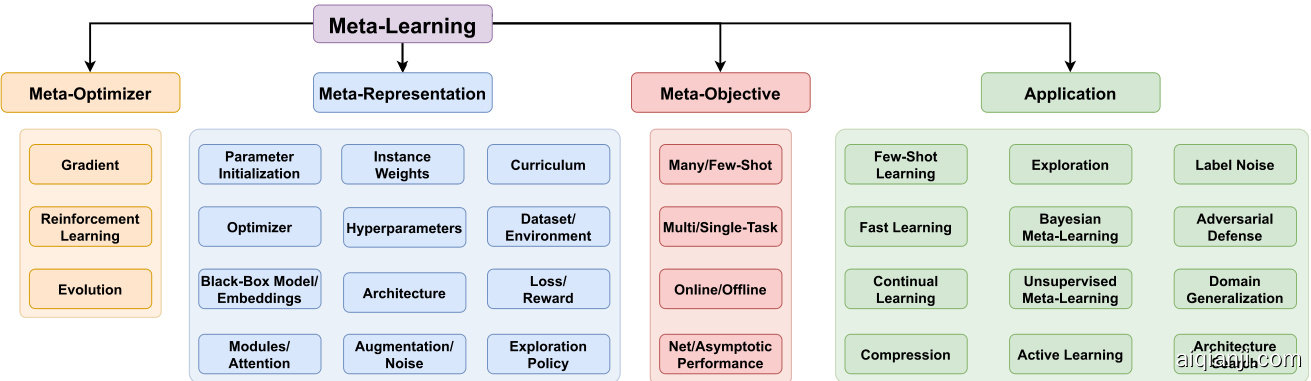
Fig. 1. Overview of the meta-learning landscape including algorithm design (meta-optimizer, meta-representation, meta-objective), and applications.

图 1: 元学习领域的概览，包括算法设计（元优化器、元表示、元目标）和应用。

Some FFMs can also be understood elegantly in terms of amortized inference in probabilistic models [45], [107], making predictions for test data $x$ as:

一些FFM也可以通过概率模型中的摊销推断 (amortized inference) 来优雅地理解 [45], [107], 对测试数据 $x$ 的预测如下:

$$
q_{\omega}(y|x,\mathcal{D}^{t r})=\int p(y|x,\theta)q_{\omega}(\theta|\mathcal{D}^{t r})d\theta,
$$

where the meta-representation $\omega$ is a network $q_{\omega}(\cdot)$ that approximates the intractable Bayesian inference for parameters $\theta$ that solve the task with training data $\mathcal{D}^{t r}$ , and the integral may be computed exactly [107], or approximated by sampling [45] or point estimate [108]. The model $\omega$ is then trained to minimise validation loss over a distribution of training tasks cf. Eq. (7).

元表示 $\omega$ 是一个网络 $q_{\omega}(\cdot)$ ，它近似于对参数 $\theta$ 的难解贝叶斯推断，这些参数通过训练数据 $\mathcal{D}^{t r}$ 解决任务，而积分可以精确计算 [107]，或通过采样 [45] 或点估计 [108] 近似。然后训练模型 $\omega$ 以最小化训练任务分布上的验证损失，参见式 (7)。

Finally, memory-augmented neural networks, with the ability to remember old data and assimilate new data quickly, typically fall in the FFM category as well [84], [85].

最后，具备记忆旧数据和快速吸收新数据能力的内存增强神经网络 (memory-augmented neural networks) 通常也属于 FFM 类别 [84], [85]。

Embedding Functions (Metric Learning). Here the meta-optimization process learns an embedding network $\omega$ that transforms raw inputs into a representation suitable for recognition by simple similarity comparison between query and support instances [23], [81], [88], [114] (e.g., with cosine similarity or euclidean distance). These methods are classified as metric learning in the conventional taxonomy (Section 3.1) but can also be seen as a special case of the feed-forward black-box models above. This can easily be seen for methods that produce logits based on the inner product of the embeddings of support and query images $x_{s}$ and $x_{q},$ namely $g_{\omega}^{T}(x_{q})\bar{g_{\omega}}(x_{s})$ [81], [114]. Here the support image generates ‘weights’ to interpret the query example, making it a special case of a FFM where the ‘hyper network’ generates a linear classifier for the query set. Vanilla methods in this family have been further enhanced by making the embedding task-conditional [99], [115], learning a more elaborate comparison metric [89], [90], or combining with gradient-based meta-learning to train other hyper-parameters such as stochastic regularize rs [116].

嵌入函数（度量学习）。这里的元优化过程学习一个嵌入网络$\omega$，将原始输入转换为适合通过查询和支持实例之间的简单相似性比较（如余弦相似度或欧几里得距离）进行识别的表示[23], [81], [88], [114]。这些方法在传统分类中被归类为度量学习（第3.1节），但也可以看作是前馈黑盒模型的一个特例。对于那些基于支持图像和查询图像的嵌入内积生成logits的方法（即$g_{\omega}^{T}(x_{q})\bar{g_{\omega}}(x_{s})$[81], [114]），这一点很容易理解。在这里，支持图像生成“权重”来解释查询示例，使其成为FFM（前馈模型）的一个特例，其中“超网络”为查询集生成一个线性分类器。该领域的原始方法通过使嵌入任务条件化[99], [115]、学习更精细的比较度量[89], [90]，或与基于梯度的元学习相结合以训练其他超参数（如随机正则化器[116]）得到了进一步改进。

Losses and Auxiliary Tasks. These approaches learn the inner task-loss $\mathcal{L}_{\omega}^{t a s k}$ for the base model (in contrast to $\mathcal{L}^{m e t a}$ , which is fixed). Loss-learning approaches typically define a function that inputs relevant quantities (e.g., predictions, labels, or model parameters) and outputs a scalar to be treated as a loss by the inner (task) optimizer. This can lead to a learned loss that is easier to optimize (less local minima) than standard alternatives [22], [25], [117], provides faster learning with improved generalization [43], [118], [119], [120], robustness to label noise [121], or whose minima corresponds to a model more robust to domain shift [42]. Loss learning methods have also been used to learn from unlabeled instances [99], [122], or to learn task as a differentiable approximation to a true nondifferentiable $\mathcal{L}^{m e t a}$ of interest such as area under precision recall curve [123].

损失函数与辅助任务。这类方法学习基础模型的内在任务损失 $\mathcal{L}_{\omega}^{t a s k}$ (区别于固定的元损失 $\mathcal{L}^{m e t a}$ )。损失学习方法通常定义一个函数，其输入相关量(如预测值、标签或模型参数)并输出一个标量，作为内部(任务)优化器的损失值。由此习得的损失函数可能比标准替代方案更易优化(局部极小值更少) [22][25][117]，能实现更快学习并提升泛化能力 [43][118][119][120]，对标签噪声具有鲁棒性 [121]，或使其极小值对应的模型对领域偏移更具适应性 [42]。损失学习方法还被用于从未标注样本中学习 [99][122]，或将任务学习作为真实不可微元损失 $\mathcal{L}^{m e t a}$ (如精确率-召回率曲线下面积 [123])的可微近似。

Loss learning also arises in generalizations of selfsupervised [124] or auxiliary task [125] learning. In these problems unsupervised predictive tasks (such as colourising pixels in vision [124], or simply changing pixels in RL [125]) are defined and optimized with the aim of improving the representation for the main task. In this case the best auxiliary task (loss) to use can be hard to predict in advance, so meta-learning can be used to select among several auxiliary losses according to their impact on improving main task learning. I.e., $\omega$ is a per-auxiliary task weight [68]. More generally, one can meta-learn an auxiliary task generator that annotates examples with auxiliary labels [126].

损失学习也出现在自监督[124]或辅助任务[125]学习的泛化中。在这些问题中，定义了无监督预测任务（例如视觉中的像素着色[124]，或简单地改变强化学习中的像素[125]），并通过优化这些任务来改进主任务的表示。在这种情况下，最佳辅助任务（损失）可能难以提前预测，因此可以使用元学习根据多个辅助损失对改进主任务学习的影响进行选择。即，$\omega$是每个辅助任务的权重[68]。更一般地，可以元学习一个辅助任务生成器，用辅助标签标注样本[126]。

Architectures. Architecture discovery has always been an important area in neural networks [38], [127], and one that is not amenable to simple exhaustive search. Meta-Learning can be used to automate this very expensive process by learning architectures. Early attempts used evolutionary algorithms to learn the topology of LSTM cells [128], while later approaches leveraged RL to generate descriptions for good CNN architectures [28]. Evolutionary Algorithms [27] can learn blocks within architectures modelled as graphs which could mutate by editing their graph. Gradient-based architecture representations have also been visited in the form of DARTS [21] where the forward pass during training consists in a softmax across the outputs of all possible layers in a given block, which are weighted by coefficients to be meta learned (i.e., $\omega$ ). During meta-test, the architecture is disc ret i zed by only keeping the layers corresponding to the highest coefficients. Recent efforts to improve DARTS have focused on more efficient different i able approximations [129], robust if ying the disc ret iz ation step [130], learning easy to adapt initialization s [131], or architecture priors [132]. See Section 5.3 for more details.

架构。架构发现一直是神经网络领域的重要研究方向[38][127]，且无法通过简单穷举搜索实现。元学习(Meta-Learning)可通过学习架构来自动化这一高成本过程。早期尝试使用进化算法学习LSTM单元的拓扑结构[128]，后续方法则利用强化学习(RL)生成优质CNN架构描述[28]。进化算法[27]可学习以图结构建模的架构模块，这些模块能通过编辑图结构实现变异。基于梯度的架构表示方法也以DARTS[21]形式出现，其训练阶段前向传播采用给定模块中所有可能层级输出的softmax加权（权重系数由元学习确定，即$\omega$）。在元测试阶段，通过仅保留最高系数对应层级来实现架构离散化。近期DARTS改进工作聚焦于：更高效的可微分近似[129]、鲁棒化离散步骤[130]、学习易适应的初始化参数[131]或架构先验[132]。详见第5.3节。

Attention Modules. have been used as comparator s in metric-based meta-learners [133], to prevent catastrophic forgetting in few-shot continual learning [134] and to summarize the distribution of text classification tasks [135].

注意力模块 (Attention Modules) 已被用作基于度量的元学习中的比较器 [133]，用于防止少样本持续学习中的灾难性遗忘 [134]，以及总结文本分类任务的分布 [135]。

Modules. Modular meta-learning [136], [137] assumes that the task agnostic knowledge $\omega$ defines a set of modules, which are re-composed in a task specific manner defined by $\theta$ in order to solve each encountered task. These strategies can be seen as meta-learning generalizations of the typical structural approaches to knowledge sharing that are well studied in multi-task and transfer learning [66], [138], and may ultimately underpin compositional learning [139].

模块化元学习 [136][137] 假设任务无关知识 $\omega$ 定义了一组模块，这些模块按照 $\theta$ 定义的任务特定方式重新组合以解决每个遇到的任务。这些策略可视为多任务和迁移学习 [66][138] 中典型知识共享结构方法的元学习泛化，并可能最终支撑组合式学习 [139]。

Hyper-Parameters. Here $\omega$ represents hyper parameters of the base learner such as regular iz ation strength [20], [69], perparameter regular iz ation [93], task-relatedness in multi-task learning [67], or sparsity strength in data cleansing [67]. Hyper parameters such as step size [69], [77], [78] can be seen as part of the optimizer, leading to an overlap between hyperparameter and optimizer learning categories.

超参数 (Hyper-Parameters)。这里 $\omega$ 表示基础学习器的超参数，例如正则化强度 (regularization strength) [20][69]、逐参数正则化 (perparameter regularization) [93]、多任务学习中的任务相关性 (task-relatedness) [67] 或数据清洗中的稀疏强度 (sparsity strength) [67]。步长 (step size) [69][77][78] 等超参数可视为优化器的一部分，这导致超参数学习和优化器学习类别之间存在重叠。

Data Augmentation and Noise. In supervised learning it is common to improve generalization by synthesizing more training data through label-preserving transformations on the existing data [13]. The data augmentation operation is wrapped up in the inner problem (Eq. (6)), and is conventionally hand-designed. However, when $\omega$ defines the data augmentation strategy, it can be learned by the outer optimization in Eq. (5) in order to maximize validation performance [140]. Since augmentation operations are often non-differentiable, this requires reinforcement learning [140], discrete gradientestimators [141], or evolutionary [142] methods. Recent attempts use meta-gradient to learn mixing proportions in mixup-based augmentation [143]. For stochastic neural networks that exploit noise internally [116], $\omega$ can define a learnable noise distribution.

数据增强与噪声。在监督学习中，通常通过对现有数据进行标签保留变换来合成更多训练数据以提升泛化能力[13]。数据增强操作被封装在内部问题(式(6))中，传统上采用人工设计方式。但当$\omega$定义数据增强策略时，可通过式(5)的外部优化进行学习，以最大化验证性能[140]。由于增强操作通常不可微分，这需要强化学习[140]、离散梯度估计器[141]或进化方法[142]。最新研究尝试利用元梯度学习基于mixup增强的混合比例[143]。对于内部利用噪声的随机神经网络[116]，$\omega$可定义可学习的噪声分布。

Minibatch Selection, Instance Weights, and Curriculum Learning. When the base algorithm is minibatch-based stochastic gradient descent, a design parameter of the learning strategy is the batch selection process. Various hand-designed methods [144] exist to improve on randomly-sampled mini batches. Meta-learning approaches can define $\omega$ as an instance selection probability [145] or neural network that picks instances [146] for inclusion in a minibatch. Related to mini-batch selection policies are methods that learn or infer per-instance loss weights for each sample in the training set [147], [148]. For example defining a base loss as $\begin{array}{r}{\mathcal{L}=\sum_{i}\omega_{i}\ell(f(x_{i}),y_{i})}\end{array}$ . This can be used to learn under label-noise by discounting noisy samples [147], [148], discount outliers [67], or correct for class imbalance [147].

小批量选择、实例权重与课程学习。当基础算法采用基于小批量的随机梯度下降时，学习策略的一个设计参数是批次选择过程。现有多种人工设计方法[144]可改进随机采样的小批量。元学习方法可将$\omega$定义为实例选择概率[145]或选择实例的神经网络[146]，用于构建小批量。与小批量选择策略相关的是那些学习或推断训练集中每个样本的逐实例损失权重的方法[147][148]，例如将基础损失定义为$\begin{array}{r}{\mathcal{L}=\sum_{i}\omega_{i}\ell(f(x_{i}),y_{i})}\end{array}$。该方法可通过降低噪声样本权重[147][148]、排除异常值[67]或校正类别不平衡[147]来实现带标签噪声的学习。

More generally, the curriculum [149] refers to sequences of data or concepts to learn that produce better performance than learning items in a random order. For instance by focusing on instances of the right difficulty while rejecting too hard or too easy (already learned) instances. Instead of defining a curriculum by hand [150], meta-learning can automate the process and select examples of the right difficulty by defining a teaching policy as the meta-knowledge and training it to optimize the student’s progress [146], [151].

更广泛地说，课程学习 [149] 指的是通过学习数据或概念的顺序，从而比随机顺序学习获得更好的性能。例如，通过专注于难度适中的实例，同时排除过难或过易（已掌握）的实例。与手动定义课程 [150] 不同，元学习可以自动化这一过程，通过将教学策略定义为元知识并训练它以优化学生的学习进度 [146] [151]，从而选择难度合适的示例。

Datasets, Labels and Environments. Another meta-representation is the support dataset itself. This departs from our initial formalization of meta-learning which considers the source datasets to be fixed (Section 2.1, Eqs. (2) and (3)). However, it can be easily understood in the bilevel view of Eqs. (5) and (6). If the validation set in the upper optimization is real and fixed, and a train set in the lower optimization is para mate rize d by $\omega,$ the training dataset can be tuned by meta-learning to optimize validation performance.

数据集、标签与环境。另一种元表示形式是支撑数据集本身。这与我们最初对元学习的形式化定义不同（第2.1节，公式(2)和(3)），后者假设源数据集是固定的。但在公式(5)和(6)的双层优化视角下很容易理解：若上层优化的验证集真实且固定，而下层优化的训练集通过参数$\omega$进行参数化，则可通过元学习调整训练数据集以优化验证性能。

In dataset distillation [152], [153], [154], the support images themselves are learned such that a few steps on them allows for good generalization on real query images. This can be used to summarize large datasets into a handful of images, which is useful for replay in continual learning where streaming datasets cannot be stored.

在数据集蒸馏 [152], [153], [154] 中，支持图像本身是通过学习得到的，使得在其上进行少量步骤就能在真实查询图像上实现良好的泛化。这种方法可用于将大型数据集概括为少量图像，对于持续学习中无法存储流式数据集的回放场景非常有用。

Rather than learning input images $x$ for fixed labels $y,$ one can also learn the input labels $y$ for fixed images $x$ . This can be used in distilling core sets [155] as in dataset distillation; or semi-supervised learning, for example to directly learn the unlabeled set’s labels to optimize validation set performance [156], [157].

与其学习固定标签 $y$ 对应的输入图像 $x$，也可以学习固定图像 $x$ 对应的输入标签 $y$。这种方法可用于提炼核心集 [155]，如数据集蒸馏；或用于半监督学习，例如直接学习未标注集的标签以优化验证集性能 [156] [157]。

In the case of sim2real learning [158] in computer vision or reinforcement learning, one uses an environment simulator to generate data for training. In this case, as detailed in Section 5.10, one can also train the graphics engine [159] or simulator [160] so as to optimize the real-data (validation) performance of the downstream model after training on data generated by that environment simulator.

在计算机视觉或强化学习中的模拟到真实学习(sim2real learning) [158]场景下，研究者会使用环境模拟器生成训练数据。如第5.10节所述，这种情况下还可以通过训练图形引擎 [159] 或模拟器 [160] 来优化下游模型在使用该环境模拟器生成的数据训练后，在真实数据(验证集)上的表现。

Discussion: Trans duct ive Representations and Methods. Most of the representations $\omega$ discussed above are parameter vectors of functions that process or generate data. However a few represent at ions mentioned are trans duct ive in the sense that the $\omega$ literally corresponds to data points [152], labels [156], or perinstance weights [67], [148]. Therefore the number of parameters in $\omega$ to meta-learn scales as the size of the dataset. While the success of these methods is a testament to the capabilities of contemporary meta-learning [154], this property may ultimately limit their s cal ability.

讨论：直推式表示与方法。上述讨论的大多数表示 $\omega$ 都是处理或生成数据的函数参数向量。然而，也有少数提到的表示是直推式的，即 $\omega$ 直接对应于数据点 [152]、标签 [156] 或逐实例权重 [67][148]。因此，元学习所需的 $\omega$ 参数数量会随数据集规模增长。虽然这些方法的成功证明了当代元学习的能力 [154]，但这一特性可能最终会限制其可扩展性。

Distinct from a trans duct ive representation are methods that are trans duct ive in the sense that they operate on the query instances as well as support instances [99], [126].

不同于传导式表示的是那些在查询实例和支持实例上操作的传导式方法 [99], [126]。

Discussion: Interpret able Symbolic Representations. A crosscutting distinction that can be made across many of the metarepresentations discussed above is between un interpret able (sub-symbolic) and human interpret able (symbolic) representations. Sub-symbolic representations, such as when $\omega$ parameterizes a neural network [15], are more common and make up the majority of studies cited above. However, meta-learning with symbolic representations is also possible, where $\omega$ represents human readable symbolic functions such as optimization program code [91]. Rather than neural loss functions [42], one can train symbolic losses $\omega$ that are defined by an expression analogous to cross-entropy [119], [121]. One can also metalearn new symbolic activation s [161] that outperform standards such as ReLU. As these meta-representations are nonsmooth, the meta-objective is non-differentiable and is harder to optimize (see Section 4.2). So the upper optimization for $\omega$ typically uses RL [91] or evolutionary algorithms [119]. However, symbolic representations may have an advantage [91], [119], [161] in their ability to generalize across task families. I. e., to span wider distributions $p(\mathcal{T})$ with a single $\omega$ during meta-training, or to have the learned $\omega$ generalize to an out of distribution task during meta-testing (see Section 6).

讨论：可解释的符号化表征。上述讨论的多种元表征之间存在一个贯穿性区别，即不可解释（亚符号）与人类可解释（符号化）表征之分。亚符号表征（例如当$\omega$参数化神经网络时[15]）更为常见，构成了前文引用的大部分研究。然而，采用符号化表征进行元学习同样可行，此时$\omega$代表人类可读的符号化函数（如优化程序代码[91]）。相较于神经损失函数[42]，可以训练由类似交叉熵的表达式定义的符号化损失$\omega$[119][121]。还能通过元学习获得优于ReLU等标准的新型符号化激活函数[161]。由于这些元表征不具备平滑性，元目标函数不可微分且更难优化（见4.2节），因此对$\omega$的上层优化通常采用强化学习[91]或进化算法[119]。但符号化表征在跨任务族泛化能力方面可能具有优势[91][119][161]，即在元训练期间用单个$\omega$覆盖更广的分布$p(\mathcal{T})$，或使学习到的$\omega$在元测试时泛化至分布外任务（见第6节）。

Discussion: Amortization. One way to relate some of the representations discussed is in terms of the degree of learning amortization entailed [45]. That is, how much task-specific optimization is performed during meta-testing versus how much learning is amortized during meta-training. Training from scratch, or conventional fine-tuning [57] perform full task-specific optimization at meta-testing, with no amortization. MAML [19] provides limited amortization by fitting an initial condition, to enable learning a new task by few-step fine-tuning. Pure FFMs [23], [88], [108] are fully amortized, with no task-specific optimization, and thus enable the fastest learning of new tasks. Meanwhile some hybrid approaches [98], [99], [109], [162] implement semiamortized learning by drawing on both feed-forward and optimization-based meta-learning in a single framework.

讨论：摊销。将所讨论的部分表征联系起来的一种方式是通过学习摊销的程度 [45]。也就是说，在元测试期间执行了多少特定任务的优化，与在元训练期间摊销了多少学习。从头开始训练或传统的微调 [57] 在元测试时执行完整的特定任务优化，没有摊销。MAML [19] 通过拟合初始条件提供有限的摊销，以实现通过少量步骤的微调来学习新任务。纯FFM [23]、[88]、[108] 是完全摊销的，没有特定任务的优化，因此能够最快地学习新任务。同时，一些混合方法 [98]、[99]、[109]、[162] 通过在单一框架中结合前馈和基于优化的元学习来实现半摊销学习。

4.2 Meta-Optimizer

4.2 元优化器

Given a choice of which facet of the learning strategy to optimize, the next axis of meta-learner design is actual outer (meta) optimization strategy to use for training $\omega$ .

给定选择优化学习策略的哪个方面后，元学习器设计的下一个轴是用于训练$\omega$的实际外部（元）优化策略。

Gradient. A large family of methods use gradient descent on the meta parameters $\omega$ [14], [19], [42], [67]. This requires computing derivatives $d\mathcal{L}^{m e t a}/d\omega$ of the outer objective, which are typically connected via the chain rule to the model parameter $\theta,$ , $d{\mathcal{L}}^{m e t a}/d\omega=(d{\mathcal{L}}^{m e t a}/d\theta)(d\theta/d\omega)$ . These methods are potentially the most efficient as they exploit analytical gradients of $\omega$ . However key challenges include: (i) Efficiently differentiating through many steps of inner optimization, for example through careful design of differentiation algorithms [20], [69], [190] and implicit different i ation [154], [163], [191], and dealing tractably with the required second-order gradients [192]. (ii) Reducing the inevitable gradient degradation problems whose severity increases with the number of inner loop optimization steps. (iii) Calculating gradients when the base learner, $\omega,$ or $\mathcal{L}^{\mathit{\hat{t}a s k}}$ include discrete or other non-differentiable operations.

梯度。一大类方法在元参数 $\omega$ 上使用梯度下降 [14], [19], [42], [67]。这需要计算外部目标的导数 $d\mathcal{L}^{m e t a}/d\omega$，这些导数通常通过链式法则与模型参数 $\theta$ 相关联，即 $d{\mathcal{L}}^{m e t a}/d\omega=(d{\mathcal{L}}^{m e t a}/d\theta)(d\theta/d\omega)$。这些方法可能是最高效的，因为它们利用了 $\omega$ 的解析梯度。然而，关键挑战包括：(i) 高效地通过内部优化的多步进行微分，例如通过精心设计微分算法 [20], [69], [190] 和隐式微分 [154], [163], [191]，并有效处理所需的二阶梯度 [192]。(ii) 减少不可避免的梯度退化问题，其严重性随着内部循环优化步骤的增加而增加。(iii) 当基础学习器 $\omega$ 或 $\mathcal{L}^{\mathit{\hat{t}a s k}}$ 包含离散或其他不可微操作时计算梯度。

Reinforcement Learning. When the base learner includes non-differentiable steps [140], or the meta-objective $\mathcal{L}^{m e t a}$ is itself non-differentiable [123], many methods [24] resort to RL to optimize the outer objective Eq. (5). This estimates the gradient $\nabla_{\omega}\mathcal{L}^{m e t a},$ typically using the policy gradient theorem. However, alleviating the requirement for different i ability in this way is typically extremely costly. Highvariance policy-gradient estimates for $\nabla_{\omega}\dot{\mathcal{L}}^{m e t a}$ mean that many outer-level optimization steps are required to converge, and each of these steps are themselves costly due to wrapping task-model optimization within them.

强化学习。当基础学习器包含不可微步骤 [140]，或元目标 $\mathcal{L}^{meta}$ 本身不可微 [123] 时，许多方法 [24] 采用强化学习 (RL) 来优化外部目标方程 (5)。这通常利用策略梯度定理来估计梯度 $\nabla_{\omega}\mathcal{L}^{meta}$。然而，以这种方式缓解可微性要求通常代价极高。针对 $\nabla_{\omega}\dot{\mathcal{L}}^{meta}$ 的高方差策略梯度估计意味着需要大量外部优化步骤才能收敛，而由于每个步骤都包含任务模型优化，这些步骤本身的计算成本也很高。

Evolution. Another approach for optimizing the metaobjective are evolutionary algorithms (EA) [17], [127], [193]. Many evolutionary algorithms have strong connections to reinforcement learning algorithms [194]. However, their performance does not depend on the length and reward sparsity of the inner optimization as for RL.

进化。另一种优化元目标的方法是进化算法 (EA) [17], [127], [193]。许多进化算法与强化学习算法有紧密联系 [194]，但其性能不像强化学习那样依赖于内部优化的长度和奖励稀疏性。

EAs are attractive for several reasons [193]: (i) They can optimize any base model and meta-objective with no differentiability constraint. (ii) Not relying on back propagation avoids both gradient degradation issues and the cost of high-order gradient computation of conventional gradient-based methods. (iii) They are highly parallel iz able for s cal ability. (iv) By maintaining a diverse population of solutions, they can avoid local minima that plague gradient-based methods [127]. However, they have a number of disadvantages: (i) The population size required increases rapidly with the number of parameters to learn. (ii) They can be sensitive to the mutation strategy and may require careful hyper parameter optimization. (iii) Their fitting ability is generally inferior to gradient-based methods, especially for large models such as CNNs.

进化算法 (EA) 具有以下优势[193]：(i) 能够优化任何基础模型和元目标，且不受可微性约束。(ii) 不依赖反向传播，既避免了梯度退化问题，又规避了传统基于梯度方法的高阶梯度计算成本。(iii) 具备高度并行化能力，可扩展性强。(iv) 通过维持多样化的解决方案种群，能够规避基于梯度方法常陷入的局部极小值问题[127]。但其也存在若干不足：(i) 所需种群规模会随待学习参数数量急剧增加。(ii) 对变异策略敏感，可能需要进行细致的超参数优化。(iii) 拟合能力通常逊于基于梯度的方法，特别是对于CNN等大型模型。

EAs are relatively more commonly applied in RL applications [25], [169] (where models are typically smaller, and inner optimization s are long and non-differentiable). However they have also been applied to learn learning rules [195], optimizers [196], architectures [27], [127] and data augmentation strategies [142] in supervised learning. They are also particularly important in learning human interpretable symbolic meta-representations [119].

进化算法 (EAs) 在强化学习应用中相对更为常见 [25], [169] (这类场景通常模型较小，且内部优化过程长且不可微分)。但它们也被用于监督学习中学习学习规则 [195]、优化器 [196]、架构 [27], [127] 以及数据增强策略 [142]。在习得人类可解释的符号化元表征 [119] 方面，进化算法也尤为重要。

Discussion. These three optimizers are also all used in conventional learning. However meta-learning comparatively more often resorts to RL and Evolution, e.g., as $\bar{\mathcal{L}}^{m e t a}$ is often non-differentiable with respect to representation $\omega$ .

讨论。这三种优化器在传统学习中也都有应用。然而元学习相对更常采用强化学习 (RL) 和进化算法，例如当 $\bar{\mathcal{L}}^{m e t a}$ 关于表示 $\omega$ 通常不可微时。

4.3 Meta-Objective and Episode Design

4.3 元目标与回合设计

The final component is to define the meta-learning goal through choice of meta-objective $\mathcal{L}^{m e t a},$ , and associated data flow between inner loop episodes and outer optimization s. Most methods define a meta-objective using a performance metric computed on a validation set, after updating the task model with $\omega$ . This is in line with classic validation set approaches to hyper parameter and model selection. However, within this framework, there are several design options:

最终组件是通过选择元目标 $\mathcal{L}^{meta}$ 来定义元学习目标，以及内部循环事件与外部优化之间的关联数据流。大多数方法使用在验证集上计算的性能指标来定义元目标，这是在用 $\omega$ 更新任务模型之后进行的。这与经典的超参数和模型选择的验证集方法一致。然而，在这一框架内，存在几种设计选项：

Many versus Few-Shot Episode Design. According to whether the goal is improving few- or many-shot performance, inner loop learning episodes may be defined with many [67], [91], [92] or few- [14], [19] examples per-task.

多样本与少样本情节设计。根据目标是提升少样本还是多样本性能，内循环学习情节可以定义为每个任务包含多个 [67], [91], [92] 或少量 [14], [19] 样本。

Fast Adaptation versus Asymptotic Performance. When validation loss is computed at the end of the inner learning episode, meta-training encourages better final performance of the base task. When it is computed as the sum of the validation loss after each inner optimization step, then meta-train- ing also encourages faster learning in the base task [78], [91], [92]. Most RL applications also use this latter setting.

快速适应与渐进性能。当在内部学习阶段结束时计算验证损失时，元训练会提升基础任务的最终性能。若将验证损失计算为每个内部优化步骤后的损失总和，则元训练还会促进基础任务中的更快学习 [78], [91], [92]。大多数强化学习应用也采用后一种设置。

Multi versus Single-Task When the goal is to tune the learner to better solve any task drawn from a given family, then inner loop learning episodes correspond to a randomly drawn task from $p(\mathcal{T})$ [19], [23], [42]. When the goal is to tune the learner to simply solve one specific task better, then the inner loop learning episodes all draw data from the same underlying task [15], [67], [173], [180], [181], [197].

多任务与单任务
当目标是调整学习器以更好地解决从给定任务族中抽取的任何任务时，内循环学习阶段对应于从 $p(\mathcal{T})$ 中随机抽取的任务 [19], [23], [42]。当目标是调整学习器以仅更好地解决一个特定任务时，内循环学习阶段均从同一底层任务中抽取数据 [15], [67], [173], [180], [181], [197]。

It is worth noting that these two meta-objectives tend to have different assumptions and value propositions. The multi-task objective obviously requires a task family $p(\mathcal{T})$ to work with, which single-task does not. Meanwhile for multi-task, the data and compute cost of meta-training can be amortized by potentially boosting the performance of multiple target tasks during meta-test; but single-task – without the new tasks for amortization – needs to improve the final solution or asymptotic performance of the current task, or meta-learn fast enough to be online.

值得注意的是，这两个元目标往往具有不同的假设和价值主张。多任务目标显然需要一个任务族 $p(\mathcal{T})$ 来支撑，而单任务则不需要。与此同时，对于多任务而言，元训练的数据和计算成本可以通过在元测试阶段提升多个目标任务的表现来分摊；但单任务由于没有新任务用于分摊成本，必须提升当前任务的最终解或渐近性能，或者实现足够快的元学习以支持在线应用。

Online versus Offline. While the classic meta-learning pipeline defines the meta-optimization as an outer-loop of the inner base learner [15], [19], some studies have attempted to preform meta-optimization online within a single base learning episode [42], [180], [197], [198]. In this case the base model $\theta$ and learner $\omega$ co-evolve during a single episode. Since there is now no set of source tasks to amortize over, meta-learning needs to be fast compared to base model learning in order to benefit sample or compute efficiency.

在线与离线。传统元学习流程将元优化定义为内部基础学习器的外循环 [15], [19], 而部分研究尝试在单个基础学习周期内在线执行元优化 [42], [180], [197], [198]。此时基础模型 $\theta$ 和学习器 $\omega$ 会在单个周期内协同演化。由于缺乏可分摊成本的源任务集，元学习必须比基础模型学习更快，才能提升样本或计算效率。

TABLE 1 Research Papers According to Our Taxonomy

Meta-Representation	Meta-Optimizer
Meta-Representation	Gradient	RL	Evolution
Initial Condition	MAML [19], [162]. MetaOptNet [163]. [76], [85], [99], [164]	[9]19]]9]99]9]	ES-MAML [168]. [169]
Optimizer	GD2 []]]]][]]]	PSD [78]. [90]
Hyperparam	HyperRep [20], HyperOpt [66], LHML [68]	MetaTrace [171]. [172]	[169] [173]
Feed-Forward model	SNAIL [38], CNAP [107]. [44], [83], [174], [175] [176]-[178]	PEARL [110].[23], [112]
Metric	MatchingNets [87], ProtoNets [22], RelationNets [88]. [89]
Loss/Reward	MetaReg [92]. [41] [120]	MetaCritic[117].[122] [179] [120]	EPG [24]. [119] [173]
Architecture	DARTS [21]. [130]	[27]	[26]
Exploration Policy		MetaCuriosity[25].[180]-[184]
Dataset/Environment	Data Distillation [151].[152] [155]	Learn to Sim [158]	[159]
InstanceWeights	MetaWeightNet[146].MentorNet[150].[147]
Data Augmentation/Noise	MetaDropout[185].[140] [115].	AutoAugment [139].	[141]
Modules	[135], [136]
AnnotationPolicy	[186], [187]	[188]

We use color to indicate salient meta-objective or application goal. We focus on the main goal of each paper for simplicity. The color code is: sample efficiency (red), learning speed (green), asymptotic performance (purple), cross-domain (blue).

表 1 根据我们分类法的研究论文

元表示	元优化器
	梯度
初始条件	MAML [19], [162], MetaOptNet [163], [76], [85], [99], [164]
优化器	GD2 []]]]][]]]
超参数	HyperRep [20], HyperOpt [66], LHML [68]
前馈模型	SNAIL [38], CNAP [107], [44], [83], [174], [175], [176]-[178]
度量	MatchingNets [87], ProtoNets [22], RelationNets [88], [89]
损失/奖励	MetaReg [92], [41], [120]
架构	DARTS [21], [130]
探索策略
数据集/环境	Data Distillation [151], [152], [155]
实例权重	MetaWeightNet [146], MentorNet [150], [147]
数据增强/噪声	MetaDropout [185], [140], [115]
模块	[135], [136]
标注策略	[186], [187]

我们使用颜色来突出元目标或应用目标。为简化起见，我们关注每篇论文的主要目标。颜色代码为：样本效率（红色）、学习速度（绿色）、渐进性能（紫色）、跨领域（蓝色）。

Other Episode Design Factors. Other operators can be inserted into the episode generation pipeline to customize meta-learning for particular applications. For example one can simulate domain-shift between training and validation to meta-optimize for good performance under domain-shift [42], [59], [93]; simulate network compression such as quantization [199] between training and validation to meta-optimize for network compress i bil it y; provide noisy labels during meta-training to optimize for label-noise robustness [94], or generate an adversarial validation set to meta-optimize for adversarial defense [95]. These opportunities are explored in more detail in the following section.

其他情节设计因素。可以在情节生成流程中插入其他算子，针对特定应用定制元学习。例如：可以模拟训练与验证间的域偏移 (domain-shift) 来元优化域偏移下的性能 [42][59][93]；模拟网络压缩 (如量化 [199]) 来元优化网络可压缩性；在元训练阶段提供噪声标签以优化标签噪声鲁棒性 [94]；或生成对抗性验证集来元优化对抗防御能力 [95]。下一节将更详细探讨这些可能性。

5 APPLICATIONS

5 应用

In this section we briefly review the ways in which metalearning has been exploited in computer vision, reinforcement learning, architecture search, and so on.

本节我们简要回顾元学习在计算机视觉、强化学习、架构搜索等领域的应用方式。

5.1 Computer Vision and Graphics

5.1 计算机视觉与图形学

Computer vision is a major consumer domain of meta-learning techniques, notably due to its impact on few-shot learning, which holds promise to deal with the challenge posed by the long-tail of concepts to recognise in vision.

计算机视觉是元学习技术的主要应用领域，尤其体现在其对少样本学习的显著影响上，这为解决视觉识别中长尾概念带来的挑战提供了可能。

5.1.1 Few-Shot Learning Methods

5.1.1 少样本 (Few-Shot) 学习方法

Few-shot learning (FSL) is extremely challenging, especially for large neural networks [1], [13], where data volume is often the dominant factor in performance [200], and training large models with small datasets leads to over fitting or nonconvergence. Meta-learning-based approaches are increasingly able to train powerful CNNs on small datasets in many vision problems. We provide a non-exhaustive representative summary as follows.

少样本学习 (Few-shot learning, FSL) 极具挑战性，尤其对于大型神经网络 [1][13] 而言，数据量往往是性能的主导因素 [200]，使用小数据集训练大模型会导致过拟合或不收敛。基于元学习的方法在众多视觉问题上越来越能够利用小数据集训练强大的CNN模型。我们提供以下非详尽代表性总结：

Classification. The most common application of meta-learning is few-shot multi-class image recognition, where the inner and outer loss functions are typically the cross entropy over training and validation data respectively [14], [23], [75], [77], [78], [88], [90], [98], [99], [102], [105], [201], [202], [203], [204]. Optimizer-centric [19], black-box [39], [81] and metric learning [88], [89], [90] models have all been considered.

分类。元学习最常见的应用是少样本多类图像识别，其中内部和外部损失函数通常分别是训练数据和验证数据的交叉熵 [14], [23], [75], [77], [78], [88], [90], [98], [99], [102], [105], [201], [202], [203], [204]。以优化器为中心 [19]、黑盒 [39], [81] 以及度量学习 [88], [89], [90] 模型都已被研究过。

This line of work has led to a steady improvement in performance compared to early methods [19], [87], [88]. However, performance is still far behind that of fully supervised methods, so there is more work to be done. Current research issues include improving cross-domain generalization [116], recognition within the joint label space defined by metatrain and meta-test classes [82], and incremental addition of new few-shot classes [134], [175].

与早期方法[19]、[87]、[88]相比，这一系列研究实现了性能的持续提升。然而，其表现仍远落后于全监督方法，因此仍需进一步探索。当前研究重点包括：提升跨域泛化能力[116]、在元训练与元测试类联合定义的标签空间内进行识别[82]，以及逐步新增少样本类别[134]、[175]。

Object Detection. Building on progress in few-shot classification, few-shot object detection [175], [205] has been demonstrated, often using feed-forward hyper networkbased approaches to embed support set images and synthesize final layer classification weights in the base model.

目标检测。基于少样本分类的进展，少样本目标检测 [175]、[205] 已被实现，通常采用基于前馈超网络的方法来嵌入支持集图像，并在基础模型中合成最终层分类权重。

Landmark Prediction. aims to locate a skeleton of key points within an image, such as such as joints of a human or robot. This is typically formulated as an image-conditional regression. For example, a MAML-based model was shown to work for human pose estimation [206], modular-metalearning was successfully applied to robotics [136], while a hyper network-based model was applied to few-shot clothes fitting for novel fashion items [175].

地标预测 (Landmark Prediction)。旨在定位图像中关键点的骨架结构，例如人体或机器人的关节。该任务通常被建模为图像条件回归问题。例如，基于MAML的模型被证明适用于人体姿态估计 [206]，模块化元学习成功应用于机器人领域 [136]，而基于超网络的模型则被用于少样本服装适配新时尚单品 [175]。

Few-Shot Object Segmentation. is important due to the cost of obtaining pixel-wise labeled images. Hyper networkbased meta-learners have been applied in the one-shot regime [207], and performance was later improved by adapting prototypical networks [208]. Other models tackle cases where segmentation has low density [209].

少样本物体分割。由于获取像素级标注图像的成本较高，这一任务具有重要意义。基于超网络的元学习方法已被应用于单样本场景[207]，随后通过改进原型网络[208]进一步提升了性能。其他模型则针对分割密度较低的情况进行了优化[209]。

Actions. Beyond still images, meta-learning has been applied to few-shot action recognition [210], [211] and prediction [212] using bot

[论文翻译]神经网络中的元学习 (Meta-Learning) 综述

原文地址：https://ieeexplore.ieee.org/stamp/stamp.jsp?tp=&arnumber=9428530

Meta-Learning in Neural Networks: A Survey

神经网络中的元学习 (Meta-Learning) 综述

1 INTRODUCTION

1 引言

2 BACKGROUND

2 背景

2.1 Formalizing Meta-Learning

2.1 形式化元学习

2.2 Historical Context of Meta-Learning

2.2 元学习的历史背景

3 TAXONOMY

3 分类体系

3.1 Previous Taxonomies

3.1 现有分类体系

3.2 Proposed Taxonomy

3.2 提出的分类法

4 SURVEY: METHODOLOGIES

4 调研：方法论

4.1 Meta-Representation

4.1 元表征 (Meta-Representation)

4.2 Meta-Optimizer

4.2 元优化器

4.3 Meta-Objective and Episode Design

4.3 元目标与回合设计

5 APPLICATIONS

5 应用

5.1 Computer Vision and Graphics

5.1 计算机视觉与图形学

5.1.1 Few-Shot Learning Methods

[论文翻译]神经网络中的元学习 (Meta-Learning) 综述

原文地址：https://ieeexplore.ieee.org/stamp/stamp.jsp?tp=&arnumber=9428530

Meta-Learning in Neural Networks: A Survey

神经网络中的元学习 (Meta-Learning) 综述

1 INTRODUCTION

1 引言

2 BACKGROUND

2 背景

2.1 Formalizing Meta-Learning

2.1 形式化元学习

2.2 Historical Context of Meta-Learning

2.2 元学习的历史背景

2.3 Related Fields

3 TAXONOMY

3 分类体系

3.1 Previous Taxonomies

3.1 现有分类体系

3.2 Proposed Taxonomy

3.2 提出的分类法

4 SURVEY: METHODOLOGIES

4 调研：方法论

4.1 Meta-Representation

4.1 元表征 (Meta-Representation)

4.2 Meta-Optimizer

4.2 元优化器

4.3 Meta-Objective and Episode Design

4.3 元目标与回合设计

5 APPLICATIONS

5 应用

5.1 Computer Vision and Graphics

5.1 计算机视觉与图形学

5.1.1 Few-Shot Learning Methods