Training Compute-Optimal Large Language Models
训练计算最优的大语言模型
We investigate the optimal model size and number of tokens for training a transformer language model under a given compute budget. We find that current large language models are significantly undertrained, a consequence of the recent focus on scaling language models whilst keeping the amount of training data constant. By training over 400 language models ranging from 70 million to over 16 billion parameters on 5 to 500 billion tokens, we find that for compute-optimal training, the model size and the number of training tokens should be scaled equally: for every doubling of model size the number of training tokens should also be doubled. We test this hypothesis by training a predicted computeoptimal model, Chinchilla, that uses the same compute budget as Gopher but with 70B parameters and $4\times$ more more data. Chinchilla uniformly and significantly outperforms Gopher (280B), GPT-3 (175B), Jurassic-1 (178B), and Megatron-Turing NLG (530B) on a large range of downstream evaluation tasks. This also means that Chinchilla uses substantially less compute for fine-tuning and inference, greatly facilitating downstream usage. As a highlight, Chinchilla reaches a state-of-the-art average accuracy of $67.5%$ on the MMLU benchmark, greater than a $7%$ improvement over Gopher.
我们研究了在给定计算预算下训练Transformer语言模型的最优模型规模和Token数量。发现当前大语言模型存在显著训练不足的问题,这是近期在保持训练数据量不变情况下盲目扩大模型规模的结果。通过训练400多个参数量从7000万到160亿不等、训练Token量从50亿到5000亿不等的语言模型,我们发现计算最优训练应保持模型规模与训练Token量的同步增长:模型规模每翻一倍,训练Token量也需相应翻倍。我们通过训练预测最优模型Chinchilla验证了这一假设,该模型与Gopher使用相同计算预算,但采用700亿参数和4倍训练数据。Chinchilla在广泛的下游评估任务中均显著优于Gopher(280B)、GPT-3(175B)、Jurassic-1(178B)和Megatron-Turing NLG(530B)。这意味着Chinchilla在微调和推理阶段所需计算量大幅减少,极大提升了下游应用便利性。值得一提的是,Chinchilla在MMLU基准测试中达到了67.5%的最新平均准确率,较Gopher提升超过7%。
1. Introduction
1. 引言
Recently a series of Large Language Models (LLMs) have been introduced (Brown et al., 2020; Lieber et al., 2021; Rae et al., 2021; Smith et al., 2022; Thoppilan et al., 2022), with the largest dense language models now having over 500 billion parameters. These large auto regressive transformers (Vaswani et al., 2017) have demonstrated impressive performance on many tasks using a variety of evaluation protocols such as zero-shot, few-shot, and fine-tuning.
近期一系列大语言模型 (LLM) 相继发布 [20][21][22][23][24],目前最大的稠密语言模型参数量已突破5000亿。这些基于自回归架构的Transformer模型 [25] 在零样本 (zero-shot)、少样本 (few-shot) 和微调等评估范式下,均展现出卓越的任务处理能力。
The compute and energy cost for training large language models is substantial (Rae et al., 2021; Thoppilan et al., 2022) and rises with increasing model size. In practice, the allocated training compute budget is often known in advance: how many accelerators are available and for how long we want to use them. Since it is typically only feasible to train these large models once, accurately estimating the best model hyper parameters for a given compute budget is critical (Tay et al., 2021).
训练大语言模型的计算和能源成本非常高昂 (Rae et al., 2021; Thoppilan et al., 2022) ,并且随着模型规模的增大而增加。在实际应用中,训练计算预算通常是预先确定的:即有多少加速器可用以及计划使用多长时间。由于通常只能对这些大型模型进行一次训练,因此准确估算给定计算预算下的最佳模型超参数至关重要 (Tay et al., 2021) 。
Kaplan et al. (2020) showed that there is a power law relationship between the number of parameters in an auto regressive language model (LM) and its performance. As a result, the field has been training larger and larger models, expecting performance improvements. One notable conclusion in Kaplan et al. (2020) is that large models should not be trained to their lowest possible loss to be compute optimal. Whilst we reach the same conclusion, we estimate that large models should be trained for many more training tokens than recommended by the authors. Specifically, given a $10\times$ increase computational budget, they suggests that the size of the model should increase $5.5\times$ while the number of training tokens should only increase $1.8\times$ . Instead, we find that model size and the number of training tokens should be scaled in equal proportions.
Kaplan等人(2020)研究表明,自回归语言模型(LM)的参数数量与其性能之间存在幂律关系。因此,该领域一直在训练越来越大的模型,以期获得性能提升。Kaplan等人(2020)的一个重要结论是:大型模型不应训练至最低可能损失值才能达到计算最优。虽然我们得出了相同结论,但我们估计大型模型应该比作者建议的训练更多训练token。具体而言,给定计算预算增加10倍时,他们建议模型规模应增加5.5倍,而训练token数量仅需增加1.8倍。但我们发现,模型规模与训练token数量应按同等比例扩展。
Following Kaplan et al. (2020) and the training setup of GPT-3 (Brown et al., 2020), many of the recently trained large models have been trained for approximately 300 billion tokens (Table 1), in line with the approach of predominantly increasing model size when increasing compute.
遵循 Kaplan 等人 (2020) 和 GPT-3 (Brown 等人, 2020) 的训练设置,近期训练的许多大模型都采用了约 3000 亿 token 的训练量 (表 1),这与通过主要增加模型规模来提升计算量的方法一致。

Figure 1 | Overlaid predictions. We overlay the predictions from our three different approaches, along with projections from Kaplan et al. (2020). We find that all three methods predict that current large models should be substantially smaller and therefore trained much longer than is currently done. In Figure A3, we show the results with the predicted optimal tokens plotted against the optimal number of parameters for fixed FLOP budgets. Chinchilla outperforms Gopher and the other large models (see Section 4.2).
图 1 | 预测结果叠加展示。我们将三种不同方法的预测结果与Kaplan等人(2020)的预测进行叠加对比。研究发现,所有方法都预测当前大模型的实际规模应明显更小,因此需要比现有训练时长更久的训练时间。在图A3中,我们展示了固定FLOP预算下最优token数量与最优参数规模的对应关系。Chinchilla模型表现优于Gopher及其他大模型(详见第4.2节)。
In this work, we revisit the question: Given a fixed FLOPs budget,1 how should one trade-off model size and the number of training tokens? To answer this question, we model the final pre-training loss2 $L(N,D)$ as a function of the number of model parameters $N$ , and the number of training tokens, $D$ . Since the computational budget $C$ is a deterministic function $\mathrm{FLOPs}(N,D)$ of the number of seen training tokens and model parameters, we are interested in minimizing $L$ under the constraint $\mathrm{FLOPs}(N,D)=C$ :
在本研究中,我们重新审视以下问题:在固定计算量 (FLOPs) 预算下,应如何权衡模型规模与训练 token 数量?为此,我们将最终预训练损失 $L(N,D)$ 建模为模型参数量 $N$ 和训练 token 量 $D$ 的函数。由于计算预算 $C$ 是训练 token 量与模型参数的确定性函数 $\mathrm{FLOPs}(N,D)$ ,我们需要在约束条件 $\mathrm{FLOPs}(N,D)=C$ 下最小化 $L$ :
$$
N_ {o p t}(C),D_ {o p t}(C)=\operatorname*{argmin}_ {N,D\mathrm{s.t.}\mathrm{FLOPs}(N,D)=C}L(N,D).
$$
$$
N_ {o p t}(C),D_ {o p t}(C)=\operatorname*{argmin}_ {N,D\mathrm{s.t.}\mathrm{FLOPs}(N,D)=C}L(N,D).
$$
The functions $N_ {o p t}(C)$ , and $D_ {o p t}(C)$ describe the optimal allocation of a computational budget 𝐶. We empirically estimate these functions based on the losses of over 400 models, ranging from under 70M to over 16B parameters, and trained on 5B to over $400\mathrm{B}$ tokens – with each model configuration trained for several different training horizons. Our approach leads to considerably different results than that of Kaplan et al. (2020). We highlight our results in Figure 1 and how our approaches differ in Section 2.
函数 $N_ {o p t}(C)$ 和 $D_ {o p t}(C)$ 描述了计算预算 𝐶 的最优分配方式。我们基于超过400个模型的损失情况对这些函数进行了实证估计,这些模型的参数量从不足7000万到超过160亿不等,并在50亿至超过 $400\mathrm{B}$ token 的数据上进行训练——每种模型配置都针对多个不同的训练周期进行了训练。我们的方法得出的结果与 Kaplan 等人 (2020) [20] 的研究存在显著差异。我们在图 1 中重点展示了我们的结果,并在第2节详细说明我们的方法有何不同。
Based on our estimated compute-optimal frontier, we predict that for the compute budget used to train Gopher, an optimal model should be 4 times smaller, while being training on 4 times more tokens. We verify this by training a more compute-optimal 70B model, called Chinchilla, on 1.4 trillion tokens. Not only does Chinchilla outperform its much larger counterpart, Gopher, but its reduced model size reduces inference cost considerably and greatly facilitates downstream uses on smaller hardware. The energy cost of a large language model is amortized through its usage for inference an fine-tuning. The benefits of a more optimally trained smaller model, therefore, extend beyond the immediate benefits of its improved performance.
根据我们估算的计算最优前沿,预测在用于训练Gopher的计算预算下,最优模型规模应缩小4倍,同时训练token数量增加4倍。我们通过训练一个计算效率更高的700亿参数模型Chinchilla(使用1.4万亿token)验证了这一结论。Chinchilla不仅显著超越其更大规模的同类模型Gopher,缩减的模型尺寸还大幅降低了推理成本,并更易于在小型硬件上进行下游应用。大语言模型的能源成本通过推理和微调过程分摊,因此更优化训练的小型模型带来的优势不仅体现在性能提升上。
Table 1 | Current LLMs. We show five of the current largest dense transformer models, their size, and the number of training tokens. Other than LaMDA (Thoppilan et al., 2022), most models are trained for approximately 300 billion tokens. We introduce Chinchilla, a substantially smaller model, trained for much longer than 300B tokens.
| Model | Size (# Parameters) | Training Tokens |
| LaMDA (Thoppilan et al., 2022) | 137 Billion | 168 Billion |
| GPT-3 (Brown et al., 2020) | 175 Billion | 300 Billion |
| Jurassic (Lieber et al.,2021) | 178 Billion | 300 Billion |
| Gopher (Rae et al.,2021) | 280 Billion | 300 Billion |
| MT-NLG530B (Smith et al.,2022) | 530 Billion | 270 Billion |
| Chinchilla | 70 Billion | 1.4 Trillion |
表 1: 当前主流大语言模型。我们列出了当前最大的五个密集Transformer模型,其参数量及训练token数。除LaMDA (Thoppilan et al., 2022)外,多数模型训练token数约为3000亿。我们提出的Chinchilla模型参数量显著更小,但训练token数远超3000亿。
| 模型 | 参数量 | 训练token数 |
|---|---|---|
| LaMDA (Thoppilan et al., 2022) | 1370亿 | 1680亿 |
| GPT-3 (Brown et al., 2020) | 1750亿 | 3000亿 |
| Jurassic (Lieber et al., 2021) | 1780亿 | 3000亿 |
| Gopher (Rae et al., 2021) | 2800亿 | 3000亿 |
| MT-NLG530B (Smith et al., 2022) | 5300亿 | 2700亿 |
| Chinchilla | 700亿 | 1.4万亿 |
2. Related Work
2. 相关工作
Large language models. A variety of large language models have been introduced in the last few years. These include both dense transformer models (Brown et al., 2020; Lieber et al., 2021; Rae et al., 2021; Smith et al., 2022; Thoppilan et al., 2022) and mixture-of-expert (MoE) models (Du et al., 2021; Fedus et al., 2021; Zoph et al., 2022). The largest dense transformers have passed 500 billion parameters (Smith et al., 2022). The drive to train larger and larger models is clear—so far increasing the size of language models has been responsible for improving the state-of-the-art in many language modelling tasks. Nonetheless, large language models face several challenges, including their overwhelming computational requirements (the cost of training and inference increase with model size) (Rae et al., 2021; Thoppilan et al., 2022) and the need for acquiring more high-quality training data. In fact, in this work we find that larger, high quality datasets will play a key role in any further scaling of language models.
大语言模型。近年来涌现了多种大语言模型,包括稠密Transformer模型 (Brown等人, 2020; Lieber等人, 2021; Rae等人, 2021; Smith等人, 2022; Thoppilan等人, 2022) 和专家混合 (MoE) 模型 (Du等人, 2021; Fedus等人, 2021; Zoph等人, 2022)。最大规模的稠密Transformer参数量已突破5000亿 (Smith等人, 2022)。训练越来越大的模型趋势显而易见——迄今为止,扩大语言模型规模一直是推动诸多语言建模任务达到最先进水平的关键因素。然而,大语言模型仍面临多重挑战,包括惊人的算力需求 (训练和推理成本随模型规模增长而增加) (Rae等人, 2021; Thoppilan等人, 2022) 以及获取更多高质量训练数据的必要性。事实上,本研究发现更大规模的高质量数据集将在语言模型的后续扩展中发挥关键作用。
Modelling the scaling behavior. Understanding the scaling behaviour of language models and their transfer properties has been important in the development of recent large models (Hernandez et al., 2021; Kaplan et al., 2020). Kaplan et al. (2020) first showed a predictable relationship between model size and loss over many orders of magnitude. The authors investigate the question of choosing the optimal model size to train for a given compute budget. Similar to us, they address this question by training various models. Our work differs from Kaplan et al. (2020) in several important ways. First, the authors use a fixed number of training tokens and learning rate schedule for all models; this prevents them from modelling the impact of these hyper parameters on the loss. In contrast, we find that setting the learning rate schedule to approximately match the number of training tokens results in the best final loss regardless of model size—see Figure A1. For a fixed learning rate cosine schedule to 130B tokens, the intermediate loss estimates (for $D^{\prime}<<130\mathrm{B}$ ) are therefore overestimates of the loss of a model trained with a schedule length matching $D^{\prime}$ . Using these intermediate losses results in underestimating the effectiveness of training models on less data than 130B tokens, and eventually contributes to the conclusion that model size should increase faster than training data size as compute budget increases. In contrast, our analysis predicts that both quantities should scale at roughly the same rate. Secondly, we include models with up to 16B parameters, as we observe that there is slight curvature in the FLOP-loss frontier (see Appendix E)—in fact, the majority of the models used in our analysis have more than 500 million parameters, in contrast the majority of runs in Kaplan et al. (2020) are significantly smaller—many being less than 100M parameters.
建模缩放行为。理解大语言模型的缩放特性及其迁移属性对近期大模型发展至关重要 (Hernandez et al., 2021; Kaplan et al., 2020)。Kaplan等人 (2020) 首次揭示了模型规模与损失函数之间跨越多个数量级的可预测关系。作者探讨了在给定计算预算下如何选择最优模型规模的问题。与我们类似,他们通过训练多种模型来研究这个问题。我们的工作与Kaplan等人 (2020) 存在几个重要差异:首先,原作者对所有模型使用固定训练token数量和学习率调度,这导致无法建模这些超参数对损失函数的影响。相反,我们发现无论模型规模如何,将学习率调度设置为与训练token数量大致匹配时能获得最佳最终损失 (见图A1)。对于固定学习率余弦调度至1300亿token的情况,中间损失估计值 (当 $D^{\prime}<<130\mathrm{B}$ 时) 会高估那些采用与 $D^{\prime}$ 匹配的调度长度训练的模型损失。使用这些中间损失值会导致低估在少于1300亿token数据上训练模型的效果,最终得出"随着计算预算增加,模型规模应比训练数据量增长更快"的结论。而我们的分析预测这两个量应以近似相同的速率缩放。其次,我们纳入了参数规模高达160亿的模型,因为观察到FLOP-损失前沿存在轻微曲率 (见附录E)——事实上,我们分析中使用的大部分模型参数超过5亿,而Kaplan等人 (2020) 的实验模型多数规模显著更小,许多不足1亿参数。
Recently, Clark et al. (2022) specifically looked in to the scaling properties of Mixture of Expert language models, showing that the scaling with number of experts diminishes as the model size increases—their approach models the loss as a function of two variables: the model size and the number of experts. However, the analysis is done with a fixed number of training tokens, as in Kaplan et al. (2020), potentially underestimating the improvements of branching.
最近,Clark等人(2022)专门研究了专家混合( Mixture of Expert)语言模型的扩展特性,表明随着模型规模增大,专家数量带来的扩展效益会递减——他们的方法将损失建模为两个变量的函数:模型规模和专家数量。不过,该分析与Kaplan等人(2020)一样采用了固定训练token数量的设定,可能低估了分支结构的改进空间。
Estimating hyper parameters for large models. The model size and the number of training tokens are not the only two parameters to chose when selecting a language model and a procedure to train it. Other important factors include learning rate, learning rate schedule, batch size, optimiser, and width-to-depth ratio. In this work, we focus on model size and the number of training steps, and we rely on existing work and provided experimental heuristics to determine the other necessary hyper parameters. Yang et al. (2021) investigates how to choose a variety of these parameters for training an auto regressive transformer, including the learning rate and batch size. McCandlish et al. (2018) finds only a weak dependence between optimal batch size and model size. Shallue et al. (2018); Zhang et al. (2019) suggest that using larger batch-sizes than those we use is possible. Levine et al. (2020) investigates the optimal depth-to-width ratio for a variety of standard model sizes. We use slightly less deep models than proposed as this translates to better wall-clock performance on our hardware.
大型模型的超参数估计。在选择语言模型及其训练流程时,模型规模和训练token数量并非唯二需要确定的参数。其他关键因素包括学习率、学习率调度策略、批大小、优化器选择以及宽深比。本研究聚焦于模型规模与训练步数,其余必要超参数则依据现有研究成果和实验启发式方法确定。Yang等人 (2021) 研究了如何为自回归Transformer选择包括学习率和批大小在内的多种参数。McCandlish等人 (2018) 发现最优批大小与模型规模之间仅存在弱相关性。Shallue等人 (2018) 和张等人 (2019) 指出可以采用比我们当前设置更大的批大小。Levine等人 (2020) 探究了不同标准模型尺寸下的最优深宽比。我们采用了比建议值稍浅的模型结构,这有助于在当前硬件上获得更好的实际运行性能。
Improved model architectures. Recently, various promising alternatives to traditional dense transformers have been proposed. For example, through the use of conditional computation large MoE models like the 1.7 trillion parameter Switch transformer (Fedus et al., 2021), the 1.2 Trillion parameter GLaM model (Du et al., 2021), and others (Artetxe et al., 2021; Zoph et al., 2022) are able to provide a large effective model size despite using relatively fewer training and inference FLOPs. However, for very large models the computational benefits of routed models seems to diminish (Clark et al., 2022). An orthogonal approach to improving language models is to augment transformers with explicit retrieval mechanisms, as done by Borgeaud et al. (2021); Guu et al. (2020); Lewis et al. (2020). This approach effectively increases the number of data tokens seen during training (by a factor of $\sim10$ in Borgeaud et al. (2021)). This suggests that the performance of language models may be more dependant on the size of the training data than previously thought.
改进的模型架构。近年来,研究者们提出了多种有望替代传统密集型Transformer的创新架构。例如,通过采用条件计算技术,大型混合专家模型(MoE)如1.7万亿参数的Switch Transformer (Fedus等人,2021)、1.2万亿参数的GLaM模型(Du等人,2021)等(Artetxe等人,2021;Zoph等人,2022)能够在相对减少训练和推理FLOPs的情况下实现更大的有效模型规模。然而对于超大规模模型,路由模型的计算优势似乎会减弱(Clark等人,2022)。另一种改进语言模型的思路是为Transformer添加显式检索机制,如Borgeaud等人(2021)、Guu等人(2020)、Lewis等人(2020)所采用的方法。这种方法能显著增加训练时接触的数据token量(在Borgeaud等人研究中提升了约10倍),这表明语言模型性能对训练数据规模的依赖可能超出既往认知。
3. Estimating the optimal parameter/training tokens allocation
3. 估算最优参数/训练token分配
We present three different approaches to answer the question driving our research: Given a fixed FLOPs budget, how should one trade-off model size and the number of training tokens? In all three cases we start by training a range of models varying both model size and the number of training tokens and use the resulting training curves to fit an empirical estimator of how they should scale. We assume a power-law relationship between compute and model size as done in Clark et al. (2022); Kaplan et al. (2020), though future work may want to include potential curvature in this relationship for large model sizes. The resulting predictions are similar for all three methods and suggest that parameter count and number of training tokens should be increased equally with more compute3— with proportions reported in Table 2. This is in clear contrast to previous work on this topic and warrants further investigation.
我们提出三种不同方法来解答驱动本研究的问题:在固定FLOPs预算下,应如何权衡模型规模与训练token数量?所有方法均从训练不同模型规模和训练token数量的系列模型开始,利用所得训练曲线拟合二者缩放关系的经验估计器。我们遵循Clark et al. (2022)和Kaplan et al. (2020)的做法,假设计算量与模型规模呈幂律关系,但未来研究可能需要考虑大模型规模下该关系的潜在曲率。三种方法得出的预测结果相似,均表明随着计算资源增加,参数量与训练token数应等比例提升——具体比例见表2。这一结论与先前研究形成鲜明对比,值得进一步探究。
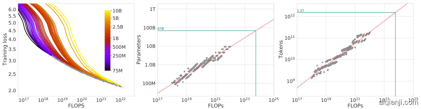
Figure 2 | Training curve envelope. On the left we show all of our different runs. We launched a range of model sizes going from 70M to 10B, each for four different cosine cycle lengths. From these curves, we extracted the envelope of minimal loss per FLOP, and we used these points to estimate the optimal model size (center) for a given compute budget and the optimal number of training tokens (right). In green, we show projections of optimal model size and training token count based on the number of FLOPs used to train Gopher $(5.76\times10^{23}.$ ).
图 2 | 训练曲线包络。左侧展示了我们所有的不同训练运行结果。我们启动了从7000万到100亿参数规模不等的多种模型,每种模型分别对应四种不同的余弦周期长度。从这些曲线中,我们提取了每单位FLOP的最小损失包络线,并利用这些数据点估算出给定计算预算下的最优模型规模(中图)以及最优训练token数量(右图)。绿色部分展示了基于训练Gopher所消耗的FLOPs $(5.76\times10^{23})$ 推算出的最优模型规模和训练token数量预测值。
3.1. Approach 1: Fix model sizes and vary number of training tokens
3.1. 方法一:固定模型规模并改变训练token数量
In our first approach we vary the number of training steps for a fixed family of models (ranging from 70M to over 10B parameters), training each model for 4 different number of training sequences. From these runs, we are able to directly extract an estimate of the minimum loss achieved for a given number of training FLOPs. Training details for this approach can be found in Appendix D.
在我们的第一种方法中,我们针对固定模型系列(参数量从7000万到超过100亿不等)调整训练步数,每个模型分别用4种不同数量的训练序列进行训练。通过这些实验,我们能够直接估算出给定训练FLOPs量时能达到的最小损失值。该方法的具体训练细节见附录D。
For each parameter count $N$ we train 4 different models, decaying the learning rate by a factor of $10\times$ over a horizon (measured in number of training tokens) that ranges by a factor of $16\times$ . Then, for each run, we smooth and then interpolate the training loss curve. From this, we obtain a continuous mapping from FLOP count to training loss for each run. Then, for each FLOP count, we determine which run achieves the lowest loss. Using these interpol ants, we obtain a mapping from any FLOP count $C$ , to the most efficient choice of model size $N$ and number of training tokens $D$ such that $\mathrm{FLOPs}(N,D)=C$ .4 At 1500 logarithmic ally spaced FLOP values, we find which model size achieves the lowest loss of all models along with the required number of training tokens. Finally, we fit power laws to estimate the optimal model size and number of training tokens for any given amount of compute (see the center and right panels of Figure 2), obtaining a relationship $N_ {o p t}\propto C^{a}$ and $D_ {o p t}\propto C^{b}$ . We find that $a=0.50$ and $b=0.50$ —as summarized in Table 2. In Section D.4, we show a head-to-head comparison at $10^{21}$ FLOPs, using the model size recommended by our analysis and by the analysis of Kaplan et al. (2020)—using the model size we predict has a clear advantage.
对于每个参数量 $N$,我们训练4个不同模型,学习率按 $10\times$ 比例衰减,训练时长(以训练token数计)跨度达 $16\times$。随后对每次运行的训练损失曲线进行平滑和插值处理,由此得到每次运行中FLOP数与训练损失的连续映射关系。接着针对每个FLOP数值,确定哪次运行能达到最低损失。通过这些插值结果,我们建立了从任意FLOP数 $C$ 到最有效模型规模 $N$ 和训练token数 $D$ 的映射关系,满足 $\mathrm{FLOPs}(N,D)=C$。在1500个对数间隔的FLOP值上,我们找出所有模型中能达到最低损失的模型规模及所需训练token数。最后通过幂律拟合估算任意计算量下的最优模型规模和训练token数(见图2中间和右侧面板),得到关系式 $N_ {o p t}\propto C^{a}$ 和 $D_ {o p t}\propto C^{b}$。我们发现 $a=0.50$ 和 $b=0.50$——如表2所示。在D.4节中,我们在 $10^{21}$ FLOPs条件下进行直接对比,使用本文分析推荐的模型规模与Kaplan等(2020)分析的推荐值——采用我们预测的模型规模具有明显优势。
3.2. Approach 2: IsoFLOP profiles
3.2. 方法二:IsoFLOP 性能曲线
In our second approach we vary the model size5 for a fixed set of 9 different training FLOP counts6 (ranging from $6\times10^{18}$ to $3\times10^{21}$ FLOPs), and consider the final training loss for each point7. in contrast with Approach 1 that considered points $(N,D,L)$ along the entire training runs. This allows us to directly answer the question: For a given FLOP budget, what is the optimal parameter count?
在我们的第二种方法中,我们针对固定的9种不同训练FLOP计算量6(范围从$6\times10^{18}$到$3\times10^{21}$ FLOPs)调整模型规模5,并观察每个数据点7的最终训练损失。这与方法1中考虑整个训练过程中$(N,D,L)$数据点形成对比,使我们能直接回答:在给定FLOP预算下,最优参数量是多少?
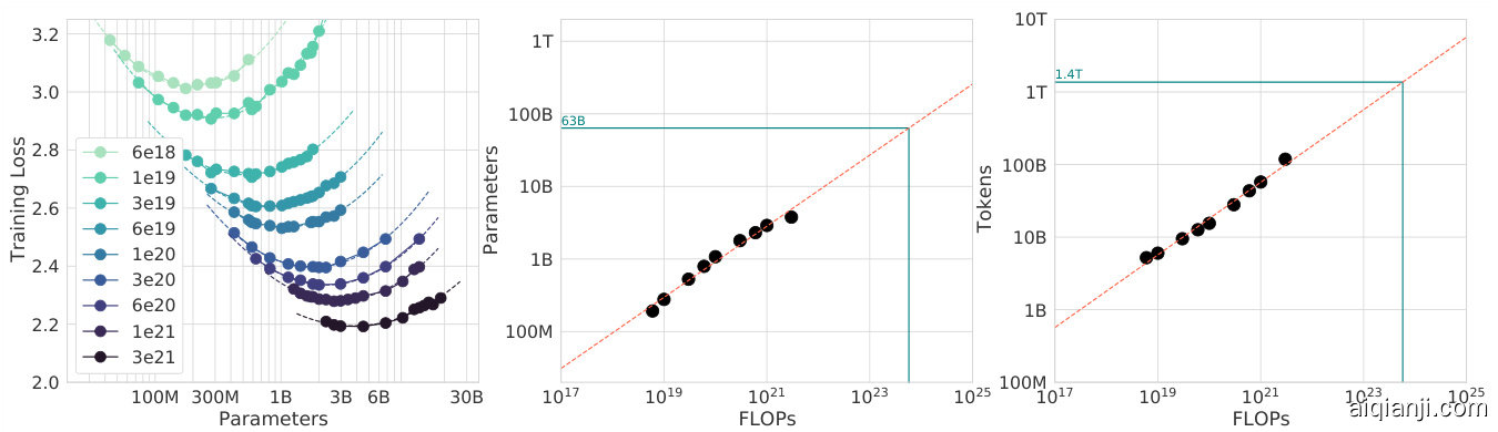
Figure 3 | IsoFLOP curves. For various model sizes, we choose the number of training tokens such that the final FLOPs is a constant. The cosine cycle length is set to match the target FLOP count. We find a clear valley in loss, meaning that for a given FLOP budget there is an optimal model to train (left). Using the location of these valleys, we project optimal model size and number of tokens for larger models (center and right). In green, we show the estimated number of parameters and tokens for an optimal model trained with the compute budget of Gopher.
图 3 | 等计算量 (IsoFLOP) 曲线。针对不同模型规模,我们选择训练 token 数量以使最终计算量 (FLOPs) 保持恒定。余弦周期长度设置为匹配目标计算量。我们发现损失函数存在明显低谷,这意味着在给定计算预算下存在最优训练模型 (左图)。利用这些低谷位置,我们推算出更大规模模型的最优参数量与 token 数量 (中图与右图)。绿色部分展示了采用 Gopher 计算预算训练时,最优模型的预估参数量与 token 数量。
For each FLOP budget, we plot the final loss (after smoothing) against the parameter count in Figure 3 (left). In all cases, we ensure that we have trained a diverse enough set of model sizes to see a clear minimum in the loss. We fit a parabola to each IsoFLOPs curve to directly estimate at what model size the minimum loss is achieved (Figure 3 (left)). As with the previous approach, we then fit a power law between FLOPs and loss-optimal model size and number of training tokens, shown in Figure 3 (center, right). Again, we fit exponents of the form $N_ {o p t}\propto C^{a}$ and $D_ {o p t}\propto C^{b}$ and we find that $a=0.49$ and $b=0.51$ —as summarized in Table 2.
对于每个FLOP预算,我们在图3(左)中绘制了最终损失(平滑处理后)与参数数量的关系。在所有情况下,我们确保训练了足够多样化的模型规模,以在损失中看到明显的最小值。我们对每条等FLOP曲线拟合抛物线,直接估计在何种模型规模下达到最小损失(图3(左))。与之前的方法类似,我们随后在FLOP与损失最优模型规模及训练token数量之间拟合了幂律关系,如图3(中、右)所示。同样,我们拟合了形式为$N_ {o p t}\propto C^{a}$和$D_ {o p t}\propto C^{b}$的指数,发现$a=0.49$和$b=0.51$——总结如表2所示。
3.3. Approach 3: Fitting a parametric loss function
3.3. 方法3:拟合参数化损失函数
Lastly, we model all final losses from experiments in Approach 1&2 as a parametric function of model parameter count and the number of seen tokens. Following a classical risk decomposition (see Section D.2), we propose the following functional form
最后,我们将方法1&2中所有实验的最终损失建模为模型参数量与所见token数的参数化函数。基于经典风险分解方法(参见附录D.2),提出以下函数形式
$$
\hat{L}(N,D)\triangleq E+\frac{A}{N^{\alpha}}+\frac{B}{D^{\beta}}.
$$
$$
\hat{L}(N,D)\triangleq E+\frac{A}{N^{\alpha}}+\frac{B}{D^{\beta}}.
$$
The first term captures the loss for an ideal generative process on the data distribution, and should correspond to the entropy of natural text. The second term captures the fact that a perfectly trained transformer with $N$ parameters under performs the ideal generative process. The final term captures the fact that the transformer is not trained to convergence, as we only make a finite number of optimisation steps, on a sample of the dataset distribution.
第一项捕捉了数据分布上理想生成过程的损失,应与自然文本的熵相对应。第二项表明,一个具有 $N$ 参数的完美训练的Transformer在性能上不及理想生成过程。最后一项则反映了Transformer未训练至收敛的事实,因为我们仅在数据集分布的样本上进行了有限次数的优化步骤。
Model fitting. To estimate $(A,B,E,\alpha,\beta)$ , we minimize the Huber loss (Huber, 1964) between the predicted and observed log loss using the L-BFGS algorithm (Nocedal, 1980):
模型拟合。为了估计 $(A,B,E,\alpha,\beta)$,我们使用 L-BFGS 算法 (Nocedal, 1980) 最小化预测对数损失与观测对数损失之间的 Huber 损失 (Huber, 1964):
$$
\operatorname*{min}_ {A,B,E,\alpha,\beta}\quad\sum_ {\mathrm{Runs}i}\mathrm{Huber}_ {\delta}\Big(\log\hat{L}(N_ {i},D_ {i})-\log L_ {i}\Big)
$$
$$
\operatorname*{min}_ {A,B,E,\alpha,\beta}\quad\sum_ {\mathrm{Runs}i}\mathrm{Huber}_ {\delta}\Big(\log\hat{L}(N_ {i},D_ {i})-\log L_ {i}\Big)
$$
We account for possible local minima by selecting the best fit from a grid of initial is at ions. The Huber loss $(\delta=10^{-3}.$ ) is robust to outliers, which we find important for good predictive performance over held-out data points. Section D.2 details the fitting procedure and the loss decomposition.
我们通过从初始参数网格中选择最佳拟合来考虑可能的局部极小值。Huber损失 $(\delta=10^{-3}.$ ) 对异常值具有鲁棒性,我们发现这对于保留数据点的良好预测性能非常重要。D.2节详细介绍了拟合过程和损失分解。

Figure 4 | Parametric fit. We fit a parametric modelling of the loss $\hat{L}(N,D)$ and display contour (left) and isoFLOP slices (right). For each isoFLOP slice, we include a corresponding dashed line in the left plot. In the left plot, we show the efficient frontier in blue, which is a line in log-log space. Specifically, the curve goes through each iso-loss contour at the point with the fewest FLOPs. We project the optimal model size given the Gopher FLOP budget to be 40B parameters.
图 4 | 参数化拟合。我们对损失函数 $\hat{L}(N,D)$ 进行参数化建模,并展示等高线图(左)和等FLOP切片图(右)。每个等FLOP切片在左图中对应一条虚线。左图中的蓝色高效边界线在双对数坐标系中呈直线,该曲线通过每个等损失等高线中FLOP最低的点。根据Gopher的FLOP预算,我们预测最优模型参数量为400亿。
Efficient frontier. We can approximate the functions $N_ {o p t}$ and $D_ {o p t}$ by minimizing the parametric loss $\hat{L}$ under the constraint $\mathrm{FLOPs}(N,D)\approx6N D$ (Kaplan et al., 2020). The resulting $N_ {o p t}$ and $D_ {o p t}$ balance the two terms in Equation (3) that depend on model size and data. By construction, they have a power-law form:
有效前沿。我们可以通过最小化参数化损失 $\hat{L}$ 来近似函数 $N_ {o p t}$ 和 $D_ {o p t}$,约束条件为 $\mathrm{FLOPs}(N,D)\approx6N D$ (Kaplan et al., 2020)。由此得到的 $N_ {o p t}$ 和 $D_ {o p t}$ 平衡了方程 (3) 中依赖于模型大小和数据的两项。根据构造,它们具有幂律形式:
$$
\begin{array}{r}{{I_ {o p t}}(C)=G\left(\displaystyle{\frac{C}{6}}\right)^{a},\quad{D_ {o p t}}(C)={G^{-1}}\left(\displaystyle{\frac{C}{6}}\right)^{b},\quad\mathrm{~where~}\quad{G}=\left(\displaystyle{\frac{\alpha A}{\beta B}}\right)^{\frac{1}{\alpha+\beta}},\quad a=\frac{\beta}{\alpha+\beta},\mathrm{~and~}b=\frac{\alpha}{\alpha+\beta}}\end{array}
$$
$$
\begin{array}{r}{{I_ {o p t}}(C)=G\left(\displaystyle{\frac{C}{6}}\right)^{a},\quad{D_ {o p t}}(C)={G^{-1}}\left(\displaystyle{\frac{C}{6}}\right)^{b},\quad\mathrm{~where~}\quad{G}=\left(\displaystyle{\frac{\alpha A}{\beta B}}\right)^{\frac{1}{\alpha+\beta}},\quad a=\frac{\beta}{\alpha+\beta},\mathrm{~and~}b=\frac{\alpha}{\alpha+\beta}}\end{array}
$$
We show contours of the fitted function $\hat{L}$ in Figure 4 (left), and the closed-form efficient computational frontier in blue. From this approach, we find that $a=0.46$ and $b=0.54$ —as summarized in Table 2.
我们在图4(左)中展示了拟合函数$\hat{L}$的等高线,并以蓝色标出闭式高效计算边界。通过该方法,我们得出$a=0.46$和$b=0.54$,如表2所示。
3.4. Optimal model scaling
3.4. 最优模型缩放
We find that the three approaches, despite using different fitting methodologies and different trained models, yield comparable predictions for the optimal scaling in parameters and tokens with FLOPs (shown in Table 2). All three approaches suggest that as compute budget increases, model size and the amount of training data should be increased in approximately equal proportions. The first and second approaches yield very similar predictions for optimal model sizes, as shown in Figure 1 and Figure A3. The third approach predicts even smaller models being optimal at larger compute budgets. We note that the observed points $(L,N,D)$ for low training FLOPs ( $\begin{array}{r}{\zeta\leqslant1e21.}\end{array}$ ) have larger residuals $\left|L-\hat{L}(N,D)\right|_ {2}^{2}$ than points with higher computational budgets. The fitted model places increased weight on the points with more FLOPs—automatically considering the low-computational budget points as outliers due to the Huber loss. As a consequence of the empirically observed negative curvature in the frontier $C\to N_ {o p t}$ (see Appendix E), this results in predicting a lower $N_ {o p t}$ than the two other approaches.
我们发现,这三种方法尽管采用了不同的拟合方法和不同的训练模型,但在参数和token的最优扩展与FLOPs的关系上得出了相似的预测(如表2所示)。所有方法都表明,随着计算预算的增加,模型大小和训练数据量应大致按相同比例增加。如图1和图A3所示,前两种方法对最优模型规模的预测非常接近。第三种方法则预测在更大计算预算下,更小的模型反而更优。值得注意的是,在低训练FLOPs($\begin{array}{r}{\zeta\leqslant1e21.}\end{array}$)情况下观测到的$(L,N,D)$点,其残差$\left|L-\hat{L}(N,D)\right|_ {2}^{2}$要高于高计算预算的点。拟合模型会赋予高FLOPs点更大的权重——由于使用了Huber损失函数,低计算预算点会被自动视为异常值。根据前沿$C\to N_ {o p t}$中实际观测到的负曲率现象(见附录E),该方法预测的$N_ {o p t}$会低于另外两种方法。
In Table 3 we show the estimated number of FLOPs and tokens that would ensure that a model of a given size lies on the compute-optimal frontier. Our findings suggests that the current generation of large language models are considerably over-sized, given their respective compute budgets, as shown in Figure 1. For example, we find that a 175 billion parameter model should be trained with a compute budget of $4.41\times10^{24}$ FLOPs and on over 4.2 trillion tokens. A 280 billion Gopher-like model is the optimal model to train given a compute budget of approximately $10^{25}$ FLOPs and should be trained on 6.8 trillion tokens. Unless one has a compute budget of $10^{26}$ FLOPs (over $250\times$ the compute used to train Gopher), a 1 trillion parameter model is unlikely to be the optimal model to train. Furthermore, the amount of training data that is projected to be needed is far beyond what is currently used to train large models, and underscores the importance of dataset collection in addition to engineering improvements that allow for model scale. While there is significant uncertainty extrapolating out many orders of magnitude, our analysis clearly suggests that given the training compute budget for many current LLMs, smaller models should have been trained on more tokens to achieve the most performant model.
表 3 展示了确保给定规模模型处于计算最优前沿所需的预估 FLOPs 和 token 数量。如图 1 所示,我们的研究表明:考虑到各自的计算预算,当前一代大语言模型的规模明显过大。例如,我们发现 1750 亿参数的模型应在 $4.41\times10^{24}$ FLOPs 的计算预算下训练,并使用超过 4.2 万亿 token。对于约 $10^{25}$ FLOPs 的计算预算,2800 亿参数规模的 Gopher 类模型是最优选择,应使用 6.8 万亿 token 进行训练。除非计算预算达到 $10^{26}$ FLOPs (超过 Gopher 训练计算量的 $250\times$ ),否则 1 万亿参数模型不太可能是最优训练选择。此外,预测所需的训练数据量远超当前大模型训练所用规模,这凸显了在工程改进实现模型扩展的同时,数据集收集的重要性。虽然外推多个数量级存在显著不确定性,但我们的分析明确表明:就当前多数大语言模型的训练计算预算而言,更小规模的模型本应通过更多 token 的训练来实现最佳性能。
Table 2 | Estimated parameter and data scaling with increased training compute. The listed values are the exponents, $a$ and $b$ , on the relationship $N_ {o p t}\propto C^{a}$ and $D_ {o p t}\propto C^{b}$ . Our analysis suggests a near equal scaling in parameters and data with increasing compute which is in clear contrast to previous work on the scaling of large models. The $10^{\mathrm{th}}$ and $90^{\mathrm{th}}$ percentiles are estimated via boots trapping data ( $80%$ of the dataset is sampled 100 times) and are shown in parenthesis.
| Approach | Coeff. a where Nopt α Ca | Coeff. b where Dopt α Cb |
| 1. Minimum over training curves | 0.50 (0.488,0.502) | 0.50 (0.501,0.512) |
| 2. IsoFLOP profiles | 0.49 (0.462,0.534) | 0.51 (0.483,0.529) |
| 3. Parametric modelling of the loss | 0.46 (0.454,0.455) | 0.54 (0.542,0.543) |
| Kaplan et al. (2020) | 0.73 | 0.27 |
表 2 | 训练计算量增加时参数与数据规模的预估比例。所列数值为关系式 $N_ {o p t}\propto C^{a}$ 和 $D_ {o p t}\propto C^{b}$ 中的指数 $a$ 与 $b$ 。我们的分析表明,随着计算量增长,参数与数据规模几乎呈同等比例扩展,这与先前关于大模型扩展的研究形成鲜明对比。通过自助法数据 (采样数据集的 $80%$ 并重复100次) 估算的第 $10^{\mathrm{th}}$ 和第 $90^{\mathrm{th}}$ 百分位数显示在括号中。
| 方法 | 系数a (Nopt ∝ Cᵃ) | 系数b (Dopt ∝ Cᵇ) |
|---|---|---|
| 1. 训练曲线最小值法 | 0.50 (0.488, 0.502) | 0.50 (0.501, 0.512) |
| 2. 等FLOP剖面法 | 0.49 (0.462, 0.534) | 0.51 (0.483, 0.529) |
| 3. 损失的参数化建模 | 0.46 (0.454, 0.455) | 0.54 (0.542, 0.543) |
| Kaplan et al. (2020) | 0.73 | 0.27 |
Table 3 | Estimated optimal training FLOPs and training tokens for various model sizes. For various model sizes, we show the projections from Approach 1 of how many FLOPs and training tokens would be needed to train compute-optimal models. The estimates for Approach $2&3$ are similar (shown in Section D.3)
| Parameters | FLOPS | FLOPs (in Gopher unit) | Tokens |
| 400Million | 1.92e+19 | 1/29,968 | 8.0 Billion |
| 1 Billion | 1.21e+20 | 1/4, 761 | 20.2 Billion |
| 10 Billion | 1.23e+22 | 1/46 | 205.1 Billion |
| 67 Billion | 5.76e+23 | 1 | 1.5 Trillion |
| 175Billion | 3.85e+24 | 6.7 | 3.7 Trillion |
| 280 Billion | 9.90e+24 | 17.2 | 5.9 Trillion |
| 520Billion | 3.43e+25 | 59.5 | 11.0 Trillion |
| 1 Trillion | 1.27e+26 | 221.3 | 21.2 Trillion |
| 10 Trillion | 1.30e+28 | 22515.9 | 216.2 Trillion |
表 3 | 不同规模模型的预估最优训练FLOPs和训练token数。针对不同规模的模型,我们展示了方法1对训练计算最优模型所需FLOPs和训练token数的预测结果。方法2&3的预估结果类似(详见D.3节)
| 参数量 | FLOPs | FLOPs (以Gopher为单位) | Token数 |
|---|---|---|---|
| 4亿 | 1.92e+19 | 1/29,968 | 80亿 |
| 10亿 | 1.21e+20 | 1/4,761 | 202亿 |
| 100亿 | 1.23e+22 | 1/46 | 2051亿 |
| 670亿 | 5.76e+23 | 1 | 1.5万亿 |
| 1750亿 | 3.85e+24 | 6.7 | 3.7万亿 |
| 2800亿 | 9.90e+24 | 17.2 | 5.9万亿 |
| 5200亿 | 3.43e+25 | 59.5 | 11.0万亿 |
| 1万亿 | 1.27e+26 | 221.3 | 21.2万亿 |
| 10万亿 | 1.30e+28 | 22515.9 | 216.2万亿 |
In Appendix C, we reproduce the IsoFLOP analysis on two additional datasets: C4 (Raffel et al., 2020a) and GitHub code (Rae et al., 2021). In both cases we reach the similar conclusion that model size and number of training tokens should be scaled in equal proportions.
在附录 C 中,我们在两个额外数据集上复现了 IsoFLOP 分析:C4 (Raffel et al., 2020a) 和 GitHub 代码库 (Rae et al., 2021)。两种情况下我们都得出相似结论:模型大小和训练 token 数量应按同等比例扩展。
4. Chinchilla
4. Chinchilla
Based on our analysis in Section 3, the optimal model size for the Gopher compute budget is somewhere between 40 and 70 billion parameters. We test this hypothesis by training a model on the larger end of this range—70B parameters—for 1.4T tokens, due to both dataset and computational efficiency considerations. In this section we compare this model, which we call Chinchilla, to Gopher and other LLMs. Both Chinchilla and Gopher have been trained for the same number of FLOPs but differ in the size of the model and the number of training tokens.
根据第3节的分析,Gopher计算预算的最佳模型规模介于400亿至700亿参数之间。出于数据集和计算效率的考虑,我们选择该范围的上限值(700亿参数)训练了一个模型(训练Token量为1.4T),以验证这一假设。本节将这一名为Chinchilla的模型与Gopher及其他大语言模型进行对比。Chinchilla与Gopher的训练FLOPs总量相同,但模型规模和训练Token量存在差异。
While pre-training a large language model has a considerable compute cost, downstream finetuning and inference also make up substantial compute usage (Rae et al., 2021). Due to being $4\times$ smaller than Gopher, both the memory footprint and inference cost of Chinchilla are also smaller.
虽然预训练大语言模型的计算成本相当高,但下游微调和推理也占据了大量计算资源 (Rae et al., 2021) 。由于 Chinchilla 的规模比 Gopher 小 4 倍,其内存占用和推理成本也更低。
4.1. Model and training details
4.1. 模型与训练细节
The full set of hyper parameters used to train Chinchilla are given in Table 4. Chinchilla uses the same model architecture and training setup as Gopher with the exception of the differences listed below.
训练Chinchilla所用的完整超参数集如表4所示。除以下列出的差异外,Chinchilla采用了与Gopher相同的模型架构和训练配置。
In Appendix G we show the impact of the various optimiser related changes between Chinchilla and Gopher. All models in this analysis have been trained on TPUv3/TPUv4 (Jouppi et al., 2017) with JAX (Bradbury et al., 2018) and Haiku (Hennigan et al., 2020). We include a Chinchilla model card (Mitchell et al., 2019) in Table A8.
在附录G中,我们展示了Chinchilla和Gopher之间各种优化器相关变更的影响。本分析中的所有模型均使用JAX (Bradbury et al., 2018) 和Haiku (Hennigan et al., 2020) 在TPUv3/TPUv4 (Jouppi et al., 2017) 上训练完成。我们在表A8中提供了Chinchilla模型卡片 (Mitchell et al., 2019)。
| Model | Layers | Number Heads | Key/Value Size | Max LR | Batch Size | |
| Gopher280B | 80 | 128 | 128 | 16,384 | 4x 10⁻⁵ | 3M → 6M |
| Chinchilla7OB | 80 | 64 | 128 | 8,192 | 1 x 10⁻⁴ | 1.5M→3M |
| 模型 | 层数 | 注意力头数 | 键值大小 | 最大学习率 | 批量大小 |
|---|---|---|---|---|---|
| Gopher280B | 80 | 128 | 128 | 16,384 | 4×10⁻⁵ |
| Chinchilla7OB | 80 | 64 | 128 | 8,192 | 1×10⁻⁴ |
Table 4 | Chinchilla architecture details. We list the number of layers, the key/value size, the bottleneck activation size $\mathrm{d}_ {\mathrm{model}}.$ , the maximum learning rate, and the training batch size ( $#$ tokens). The feed-forward size is always set to $4\times\mathrm{d}_ {\mathrm{model}}$ . Note that we double the batch size midway through training for both Chinchilla and Gopher.
表 4 | Chinchilla 架构细节。我们列出了层数、键/值大小、瓶颈激活大小 $\mathrm{d}_ {\mathrm{model}}$ 、最大学习率以及训练批次大小 ( $#$ tokens)。前馈大小始终设置为 $4\times\mathrm{d}_ {\mathrm{model}}$ 。请注意,在训练中途我们将 Chinchilla 和 Gopher 的批次大小都翻倍了。
Table 5 | All evaluation tasks. We evaluate Chinchilla on a collection of language modelling along with downstream tasks. We evaluate on largely the same tasks as in Rae et al. (2021), to allow for direct comparison.
| # Tasks | Examples | |
| Language Modelling | 20 | WikiText-103, The Pile: PG-19, arXiv, FreeLaW, ... |
| Reading Comprehension | 3 | RACE-m,RACE-h,LAMBADA |
| QuestionAnswering | 3 | Natural Questions, TriviaQA, TruthfulQA |
| Common Sense | 5 | HellaSwag, Winogrande, PIQA, SIQA, BoolQ |
| MMLU | 57 | High School Chemistry, Astronomy, Clinical Knowledge, .. . |
| BIG-bench | 62 | Causal Judgement, Epistemic Reasoning, Temporal Sequences, |
表 5 | 所有评估任务。我们在语言建模和下游任务集合上对Chinchilla进行评估。评估任务与Rae等人 (2021) 的研究基本一致,以便直接比较。
| # 任务 | 示例 | |
|---|---|---|
| 语言建模 | 20 | WikiText-103, The Pile: PG-19, arXiv, FreeLaW, ... |
| 阅读理解 | 3 | RACE-m, RACE-h, LAMBADA |
| 问答 | 3 | Natural Questions, TriviaQA, TruthfulQA |
| 常识推理 | 5 | HellaSwag, Winogrande, PIQA, SIQA, BoolQ |
| MMLU | 57 | High School Chemistry, Astronomy, Clinical Knowledge, ... |
| BIG-bench | 62 | Causal Judgement, Epistemic Reasoning, Temporal Sequences |
4.2. Results
4.2. 结果
We perform an extensive evaluation of Chinchilla, comparing against various large language models. We evaluate on a large subset of the tasks presented in Rae et al. (2021), shown in Table 5. As the focus of this work is on optimal model scaling, we included a large representative subset, and introduce a few new evaluations to allow for better comparison to other existing large models. The evaluation details for all tasks are the same as described in Rae et al. (2021).
我们对Chinchilla进行了广泛评估,并与多种大语言模型进行对比。评估基于Rae等人(2021) 提出的任务集中大部分子集,如表5所示。由于本研究聚焦于最优模型缩放,我们纳入了具有代表性的大型子集,并引入若干新评估指标以提升与现有大模型的对比效果。所有任务的评估细节均与Rae等人(2021) 所述保持一致。
4.2.1. Language modelling
4.2.1. 语言建模

Figure 5 | Pile Evaluation. For the different evaluation sets in The Pile (Gao et al., 2020), we show the bits-per-byte (bpb) improvement (decrease) of Chinchilla compared to Gopher. On all subsets, Chinchilla outperforms Gopher.
图 5 | Pile评估结果。针对The Pile (Gao et al., 2020)中的不同评估集,我们展示了Chinchilla相比Gopher在每字节比特数(bpb)上的改进(降低)。在所有子集上,Chinchilla均优于Gopher。
Chinchilla significantly outperforms Gopher on all evaluation subsets of The Pile (Gao et al., 2020), as shown in Figure 5. Compared to Jurassic-1 (178B) Lieber et al. (2021), Chinchilla is more performant on all but two subsets– dm mathematics and ubuntu_irc– see Table A5 for a raw bits-per-byte comparison. On Wikitext 103 (Merity et al., 2017), Chinchilla achieves a perplexity of 7.16 compared to 7.75 for Gopher. Some caution is needed when comparing Chinchilla with Gopher on these language modelling benchmarks as Chinchilla is trained on $4\times$ more data than Gopher and thus train/test set leakage may artificially enhance the results. We thus place more emphasis on other tasks for which leakage is less of a concern, such as MMLU (Hendrycks et al., 2020) and BIG-bench (BIG-bench collaboration, 2021) along with various closed-book question answering and common sense analyses.
如图5所示,Chinchilla在The Pile (Gao et al., 2020)的所有评估子集上均显著优于Gopher。与Jurassic-1 (178B) (Lieber et al., 2021)相比,Chinchilla仅在dm mathematics和ubuntu_irc两个子集上表现稍逊,原始每字节比特数对比详见表A5。在Wikitext 103 (Merity et al., 2017)上,Chinchilla的困惑度达到7.16,而Gopher为7.75。需要注意的是,由于Chinchilla的训练数据量是Gopher的4倍,在这些语言建模基准测试中进行比较时,训练集/测试集的数据泄露可能会人为提升结果。因此我们更关注数据泄露影响较小的其他任务,例如MMLU (Hendrycks et al., 2020)、BIG-bench (BIG-bench collaboration, 2021)以及各类闭卷问答和常识分析任务。
Table 6 | Massive Multitask Language Understanding (MMLU). We report the average 5-shot accuracy over 57 tasks with model and human accuracy comparisons taken from Hendrycks et al. (2020). We also include the average prediction for state of the art accuracy in June 2022/2023 made by 73 competitive human forecasters in Steinhardt (2021).
| Random Average human rater GPT-35-shot | 25.0% 34.5% 43.9% |
| Gopher5-shot | 60.0% |
| Chinchilla5-shot Average human expert performance | 67.6% |
| June2022Forecast | 89.8% |
| June2023Forecast | 57.1% 63.4% |
表 6 | 大规模多任务语言理解 (MMLU)。我们报告了57个任务上的平均5样本准确率,并与Hendrycks等人 (2020) 提供的模型及人类准确率进行对比。同时包含Steinhardt (2021) 中73位竞争性人类预测者对2022/2023年6月最先进准确率的平均预测值。
| 随机平均人类评分者 GPT-35样本 | 25.0% 34.5% 43.9% |
| Gopher5样本 | 60.0% |
| Chinchilla5样本 平均人类专家表现 | 67.6% |
| 2022年6月预测 | 89.8% |
| 2023年6月预测 | 57.1% 63.4% |
4.2.2. MMLU
4.2.2. MMLU
The Massive Multitask Language Understanding (MMLU) benchmark (Hendrycks et al., 2020) consists of a range of exam-like questions on academic subjects. In Table 6, we report Chinchilla’s average 5-shot performance on MMLU (the full breakdown of results is shown in Table A6). On this benchmark, Chinchilla significantly outperforms Gopher despite being much smaller, with an average accuracy of $67.6%$ (improving upon Gopher by $7.6%$ ). Remarkably, Chinchilla even outperforms the expert forecast for June 2023 of $63.4%$ accuracy (see Table 6) (Steinhardt, 2021). Furthermore, Chinchilla achieves greater than $90%$ accuracy on 4 different individual tasks– high school gov and politics, international law, sociology, and us foreign policy. To our knowledge, no other model has achieved greater than $90%$ accuracy on a subset.
大规模多任务语言理解 (MMLU) 基准测试 (Hendrycks et al., 2020) 包含一系列学术科目类考试题目。在表 6 中,我们报告了 Chinchilla 在 MMLU 上的平均 5-shot 表现 (完整结果分解见表 A6)。在该基准测试中,尽管模型规模小得多,Chinchilla 仍显著优于 Gopher,平均准确率达到 $67.6%$ (比 Gopher 提升 $7.6%$)。值得注意的是,Chinchilla 甚至超越了 2023 年 6 月专家预测的 $63.4%$ 准确率 (见表 6) (Steinhardt, 2021)。此外,Chinchilla 在 4 个独立任务上取得了超过 $90%$ 的准确率——高中政治、国际法、社会学和美国外交政策。据我们所知,目前没有其他模型能在子任务上实现超过 $90%$ 的准确率。
In Figure 6, we show a comparison to Gopher broken down by task. Overall, we find that Chinchilla improves performance on the vast majority of tasks. On four tasks (college mathematics, econometrics, moral scenarios, and formal logic) Chinchilla under performs Gopher, and there is no change in performance on two tasks.
在图6中,我们展示了按任务分类与Gopher的对比结果。总体而言,我们发现Chinchilla在绝大多数任务上表现更优。在四个任务(大学数学、计量经济学、道德场景和形式逻辑)中Chinchilla表现不及Gopher,另有两个任务表现持平。
4.2.3. Reading comprehension
4.2.3. 阅读理解
On the final word prediction dataset LAMBADA (Paperno et al., 2016), Chinchilla achieves $77.4%$ accuracy, compared to $74.5%$ accuracy from Gopher and $76.6%$ from MT-NLG 530B (see Table 7). On RACE-h and RACE-m (Lai et al., 2017), Chinchilla greatly outperforms Gopher, improving accuracy by more than $10%$ in both cases—see Table 7.
在最终词预测数据集LAMBADA (Paperno等人,2016)上,Chinchilla达到了77.4%的准确率,而Gopher为74.5%,MT-NLG 530B为76.6%(见表7)。在RACE-h和RACE-m (Lai等人,2017)上,Chinchilla大幅超越Gopher,两项准确率均提升超过10%——见表7。
4.2.4. BIG-bench
4.2.4. BIG-bench
We analysed Chinchilla on the same set of BIG-bench tasks (BIG-bench collaboration, 2021) reported in Rae et al. (2021). Similar to what we observed in MMLU, Chinchilla outperforms Gopher on the vast majority of tasks (see Figure 7). We find that Chinchilla improves the average performance by $10.7%$ , reaching an accuracy of $65.1%$ versus $54.4%$ for Gopher. Of the 62 tasks we consider, Chinchilla performs worse than Gopher on only four—crash blossom, dark humor detection,
我们在Rae等人(2021)报告的同一组BIG-bench任务(BIG-bench collaboration, 2021)上分析了Chinchilla。与在MMLU中观察到的类似,Chinchilla在绝大多数任务上表现优于Gopher(见图7)。我们发现Chinchilla将平均性能提高了$10.7%$,准确率达到$65.1%$,而Gopher为$54.4%$。在我们考虑的62项任务中,Chinchilla仅在四项任务上表现不如Gopher——crash blossom、dark humor detection、

Figure 6 | MMLU results compared to Gopher We find that Chinchilla outperforms Gopher by $7.6%$ on average (see Table 6) in addition to performing better on 51/57 individual tasks, the same on 2/57, and worse on only 4/57 tasks.
图 6 | Chinchilla与Gopher在MMLU上的对比结果 我们发现Chinchilla平均表现优于Gopher达7.6%(见表6),在57项任务中的51项表现更佳,2项持平,仅4项表现稍逊。
| Chinchilla | Gopher | GPT-3 | MT-NLG530B | |
| LAMBADAZero-Shot | 77.4 | 74.5 | 76.2 | 76.6 |
| RACE-m Few-Shot | 86.8 | 75.1 | 58.1 | |
| RACE-h Few-Shot | 82.3 | 71.6 | 46.8 | 47.9 |
| Chinchilla | Gopher | GPT-3 | MT-NLG530B | |
|---|---|---|---|---|
| LAMBADA (零样本) | 77.4 | 74.5 | 76.2 | 76.6 |
| RACE-m (少样本) | 86.8 | 75.1 | 58.1 | |
| RACE-h (少样本) | 82.3 | 71.6 | 46.8 | 47.9 |
Table 7 | Reading comprehension. On RACE-h and RACE-m (Lai et al., 2017), Chinchilla considerably improves performance over Gopher. Note that GPT-3 and MT-NLG 530B use a different prompt format than we do on RACE-h/m, so results are not comparable to Gopher and Chinchilla. On LAMBADA (Paperno et al., 2016), Chinchilla outperforms both Gopher and MT-NLG 530B.
表 7 | 阅读理解。在 RACE-h 和 RACE-m (Lai et al., 2017) 上,Chinchilla 相比 Gopher 显著提升了性能。需要注意的是,GPT-3 和 MT-NLG 530B 在 RACE-h/m 上使用了与我们不同的提示格式,因此结果无法与 Gopher 和 Chinchilla 直接比较。在 LAMBADA (Paperno et al., 2016) 任务中,Chinchilla 的表现优于 Gopher 和 MT-NLG 530B。
mathematical induction and logical arg s. Full accuracy results for Chinchilla can be found in Table A7.
数学归纳法和逻辑论证。Chinchilla 的完整准确率结果见表 A7。
4.2.5. Common sense
4.2.5. 常识
We evaluate Chinchilla on various common sense benchmarks: PIQA (Bisk et al., 2020), SIQA (Sap et al., 2019), Winogrande (Sakaguchi et al., 2020), HellaSwag (Zellers et al., 2019), and BoolQ (Clark et al., 2019). We find that Chinchilla outperforms both Gopher and GPT-3 on all tasks and outperforms MT-NLG 530B on all but one task—see Table 8.
我们在多个常识基准上评估Chinchilla:PIQA [20]、SIQA [19]、Winogrande [20]、HellaSwag [19]和BoolQ [19]。结果表明,Chinchilla在所有任务上都优于Gopher和GPT-3,且除一项任务外均超越MT-NLG 530B模型——详见表8。
On TruthfulQA (Lin et al., 2021), Chinchilla reaches $43.6%$ , $58.5%$ , and $66.7%$ accuracy with 0-shot, 5-shot, and 10-shot respectively. In comparison, Gopher achieved only $29.5%$ 0-shot and $43.7%$ 10-shot accuracy. In stark contrast with the findings of Lin et al. (2021), the large improvements ( $74.1%$ in 0-shot accuracy) achieved by Chinchilla suggest that better modelling of the pre-training data alone can lead to substantial improvements on this benchmark.
在TruthfulQA (Lin et al., 2021) 测试中,Chinchilla 在零样本、5样本和10样本设置下分别达到 $43.6%$、$58.5%$ 和 $66.7%$ 的准确率。相比之下,Gopher 仅获得 $29.5%$ 的零样本准确率和 $43.7%$ 的10样本准确率。与Lin等人 (2021) 的研究结果形成鲜明对比的是,Chinchilla 实现的显著提升 (零样本准确率提高 $74.1%$) 表明,仅通过对预训练数据进行更好的建模,就能在该基准测试上取得实质性进步。

Figure 7 | BIG-bench results compared to Gopher Chinchilla out performs Gopher on all but four BIG-bench tasks considered. Full results are in Table A7.
图 7 | BIG-bench基准测试结果与Gopher对比 Chinchilla在除四项BIG-bench任务外的所有任务上均优于Gopher。完整结果见表 A7。
4.2.6. Closed-book question answering
4.2.6. 闭卷问答
Results on closed-book question answering benchmarks are reported in Table 9. On the Natural Questions dataset (Kwiatkowski et al., 2019), Chinchilla achieves new closed-book SOTA accuracies: $31.5%$ 5-shot and $35.5%$ 64-shot, compared to $21%$ and $28%$ respectively, for Gopher. On TriviaQA (Joshi et al., 2017) we show results for both the filtered (previously used in retrieval and open-book work) and unfiltered set (previously used in large language model evaluations). In both cases, Chinchilla substantially out performs Gopher. On the filtered version, Chinchilla lags behind the open book SOTA (Izacard and Grave, 2020) by only $7.9%$ . On the unfiltered set, Chinchilla outperforms GPT-3—see Table 9.
闭卷问答基准测试结果见表 9。在 Natural Questions 数据集 (Kwiatkowski et al., 2019) 上,Chinchilla 实现了新的闭卷 SOTA 准确率:5-shot 达到 $31.5%$,64-shot 达到 $35.5%$,而 Gopher 分别为 $21%$ 和 $28%$。在 TriviaQA (Joshi et al., 2017) 上,我们同时展示了过滤集(先前用于检索和开卷研究)和未过滤集(先前用于大语言模型评估)的结果。两种情况下,Chinchilla 都大幅超越 Gopher。在过滤版本中,Chinchilla 仅落后开卷 SOTA (Izacard and Grave, 2020) $7.9%$。在未过滤集上,Chinchilla 表现优于 GPT-3——见表 9。
4.2.7. Gender bias and toxicity
4.2.7. 性别偏见与毒性内容
Large Language Models carry potential risks such as outputting offensive language, propagating social biases, and leaking private information (Bender et al., 2021; Weidinger et al., 2021). We expect Chinchilla to carry risks similar to Gopher because Chinchilla is trained on the same data, albeit with slightly different relative weights, and because it has a similar architecture. Here, we examine gender bias (particularly gender and occupation bias) and generation of toxic language. We select a few common evaluations to highlight potential issues, but stress that our evaluations are not comprehensive and much work remains to understand, evaluate, and mitigate risks in LLMs.
大语言模型存在输出冒犯性言论、传播社会偏见和泄露隐私信息等潜在风险 (Bender et al., 2021; Weidinger et al., 2021)。由于Chinchilla采用与Gopher相同的数据集(仅权重分配略有差异)且架构相似,我们预计其风险特征与Gopher相近。本文重点考察性别偏见(特别是性别与职业关联偏见)和有害语言生成问题。我们选取了几种常见评估方法来揭示潜在风险,但需要强调的是,这些评估并不全面,在理解、评估和缓解大语言模型风险方面仍有大量工作亟待完成。
Table 8 | Zero-shot comparison on Common Sense benchmarks. We show a comparison between Chinchilla, Gopher, and MT-NLG 530B on various Common Sense benchmarks. We see that Chinchilla matches or outperforms Gopher and GPT-3 on all tasks. On all but one Chinchilla outperforms the much larger MT-NLG 530B model.
| Chinchilla | Gopher | GPT-3 | MT-NLG530B | Supervised SOTA | |
| HellaSWAG | 80.8% | 79.2% | 78.9% | 80.2% | 93.9% |
| PIQA | 81.8% | 81.8% | 81.0% | 82.0% | 90.1% |
| Winogrande | 74.9% | 70.1% | 70.2% | 73.0% | 91.3% |
| SIQA | 51.3% | 50.6% | 83.2% | ||
| BoolQ | 83.7% | 79.3% | 60.5% | 78.2% | 91.4% |
表 8 | 常识基准测试的零样本比较。我们展示了 Chinchilla、Gopher 和 MT-NLG 530B 在各种常识基准测试中的对比。可以看到 Chinchilla 在所有任务上都达到或超越了 Gopher 和 GPT-3 的表现。除一项外,Chinchilla 在所有测试中都优于规模更大的 MT-NLG 530B 模型。
| Chinchilla | Gopher | GPT-3 | MT-NLG530B | Supervised SOTA | |
|---|---|---|---|---|---|
| HellaSWAG | 80.8% | 79.2% | 78.9% | 80.2% | 93.9% |
| PIQA | 81.8% | 81.8% | 81.0% | 82.0% | 90.1% |
| Winogrande | 74.9% | 70.1% | 70.2% | 73.0% | 91.3% |
| SIQA | 51.3% | 50.6% | 83.2% | ||
| BoolQ | 83.7% | 79.3% | 60.5% | 78.2% | 91.4% |
Table 9 | Closed-book question answering. For Natural Questions (Kwiatkowski et al., 2019) and TriviaQA (Joshi et al., 2017), Chinchilla outperforms Gopher in all cases. On Natural Questions, Chinchilla outperforms GPT-3. On TriviaQA we show results on two different evaluation sets to allow for comparison to GPT-3 and to open book SOTA (FiD $+$ Distillation (Izacard and Grave, 2020)).
| Method | Chinchilla | Gopher | GPT-3 | SOTA (open book) | |
| Natural Questions (dev) | O-shot | 16.6% | 10.1% | 14.6% | 54.4% |
| 5-shot | 31.5% | 24.5% | |||
| 64-shot | 35.5% | 28.2% | 29.9% | ||
| TriviaQA (unfiltered, test) | O-shot | 67.0% | 52.8% | 64.3 % | |
| 5-shot | 73.2% | 63.6% | |||
| 64-shot | 72.3% | 61.3% | 71.2% | ||
| TriviaQA (filtered, dev) | O-shot | 55.4% | 43.5% | 72.5% | |
| 5-shot | 64.1% | 57.0% | |||
| 64-shot | 64.6% | 57.2% |
表 9 | 闭卷问答。在 Natural Questions (Kwiatkowski 等人, 2019) 和 TriviaQA (Joshi 等人, 2017) 上, Chinchilla 在所有情况下都优于 Gopher。在 Natural Questions 上, Chinchilla 优于 GPT-3。在 TriviaQA 上, 我们展示了两组不同评估集的结果, 以便与 GPT-3 和开卷 SOTA (FiD $+$ Distillation (Izacard 和 Grave, 2020)) 进行比较。
| 方法 | Chinchilla | Gopher | GPT-3 | SOTA (开卷) | |
|---|---|---|---|---|---|
| Natural Questions (dev) | 零样本 | 16.6% | 10.1% | 14.6% | 54.4% |
| 少样本 (5) | 31.5% | 24.5% | |||
| 少样本 (64) | 35.5% | 28.2% | 29.9% | ||
| TriviaQA (未过滤, 测试) | 零样本 | 67.0% | 52.8% | 64.3% | |
| 少样本 (5) | 73.2% | 63.6% | |||
| 少样本 (64) | 72.3% | 61.3% | 71.2% | ||
| TriviaQA (过滤, dev) | 零样本 | 55.4% | 43.5% | 72.5% | |
| 少样本 (5) | 64.1% | 57.0% | |||
| 少样本 (64) | 64.6% | 57.2% |
Gender bias. As discussed in Rae et al. (2021), large language models reflect contemporary and historical discourse about different groups (such as gender groups) from their training dataset, and we expect the same to be true for Chinchilla. Here, we test if potential gender and occupation biases manifest in unfair outcomes on co reference resolutions, using the Winogender dataset (Rudinger et al., 2018) in a zero-shot setting. Winogender tests whether a model can correctly determine if a pronoun refers to different occupation words. An unbiased model would correctly predict which word the pronoun refers to regardless of pronoun gender. We follow the same setup as in Rae et al. (2021) (described further in Section H.3).
性别偏见。如 Rae 等人 (2021) 所述,大语言模型会从训练数据集中反映关于不同群体(如性别群体)的当代和历史论述,我们预计 Chinchilla 也存在同样现象。此处我们采用 Winogender 数据集 (Rudinger 等人, 2018) 在零样本设置下,测试潜在的性别与职业偏见是否会在共指消解中导致不公正结果。Winogender 用于检验模型能否正确判断代词所指的不同职业词汇,无偏见模型应能准确预测代词所指对象而不受代词性别影响。实验设置与 Rae 等人 (2021) 保持一致(详见 H.3 章节说明)。
As shown in Table 10, Chinchilla correctly resolves pronouns more frequently than Gopher across all groups. Interestingly, the performance increase is considerably smaller for male pronouns (increase of $3.2%$ ) than for female or neutral pronouns (increases of $8.3%$ and $9.2%$ respectively). We also consider gotcha examples, in which the correct pronoun resolution contradicts gender stereotypes (determined by labor statistics). Again, we see that Chinchilla resolves pronouns more accurately than Gopher. When breaking up examples by male/female gender and gotcha/not gotcha, the largest improvement is on female gotcha examples (improvement of $10%$ ). Thus, though Chinchilla uniformly overcomes gender stereotypes for more co reference examples than Gopher, the rate of improvement is higher for some pronouns than others, suggesting that the improvements conferred by using a more compute-optimal model can be uneven.
如表 10 所示,Chinchilla 在所有组别中正确解析代词的频率都高于 Gopher。有趣的是,男性代词的性能提升 ($3.2%$) 明显小于女性或中性代词 (分别为 $8.3%$ 和 $9.2%$)。我们还考虑了陷阱示例,其中正确的代词解析与性别刻板印象 (由劳动统计数据确定) 相矛盾。同样,我们发现 Chinchilla 比 Gopher 更准确地解析代词。当按男性/女性性别和陷阱/非陷阱分类示例时,最大的改进出现在女性陷阱示例上 (提升 $10%$)。因此,尽管 Chinchilla 在更多共指示例上一致性地克服了性别刻板印象,但某些代词的改进率高于其他代词,这表明使用计算更优化的模型所带来的改进可能是不均衡的。
Sample toxicity. Language models are capable of generating toxic language—including insults, hate speech, profanities and threats (Gehman et al., 2020; Rae et al., 2021). While toxicity is an umbrella term, and its evaluation in LMs comes with challenges (Welbl et al., 2021; Xu et al., 2021), automatic classifier scores can provide an indication for the levels of harmful text that a LM generates. Rae et al. (2021) found that improving language modelling loss by increasing the number of model parameters has only a negligible effect on toxic text generation (unprompted); here we analyze whether the same holds true for a lower LM loss achieved via more compute-optimal training. Similar to the protocol of Rae et al. (2021), we generate 25,000 unprompted samples from Chinchilla, and compare their Perspective API toxicity score distribution to that of Gopher-generated samples. Several summary statistics indicate an absence of major differences: the mean (median) toxicity score for Gopher is 0.081 (0.064), compared to 0.087 (0.066) for Chinchilla, and the $95^{\mathrm{th}}$ percentile scores are 0.230 for Gopher, compared to 0.238 for Chinchilla. That is, the large majority of generated samples are classified as non-toxic, and the difference between the models is negligible. In line with prior findings (Rae et al., 2021), this suggests that toxicity levels in unconditional text generation are largely independent of the model quality (measured in language modelling loss), i.e. that better models of the training dataset are not necessarily more toxic.
样本毒性。语言模型能够生成包含侮辱、仇恨言论、亵渎和威胁的有害内容 (Gehman et al., 2020; Rae et al., 2021) 。虽然毒性是一个宽泛概念,且其在大语言模型中的评估存在挑战 (Welbl et al., 2021; Xu et al., 2021) ,但自动分类器评分可以反映大语言模型生成有害文本的水平。Rae et al. (2021) 发现,通过增加模型参数来提升语言建模损失对毒性文本生成 (无提示场景) 的影响微乎其微;本文则分析通过更优化的计算训练实现更低语言建模损失时,这一结论是否依然成立。参照 Rae et al. (2021) 的实验方案,我们从 Chinchilla 生成 25,000 个无提示样本,并将其 Perspective API 毒性分数分布与 Gopher 生成样本进行对比。多项统计指标显示两者无显著差异:Gopher 的平均 (中位数) 毒性分数为 0.081 (0.064) ,而 Chinchilla 为 0.087 (0.066) ;Gopher 的 95$^{\mathrm{th}}$ 百分位分数为 0.230,Chinchilla 为 0.238。这表明绝大多数生成样本被归类为非毒性,且模型间差异可忽略不计。这与先前研究结论 (Rae et al., 2021) 一致:无条件文本生成中的毒性水平基本与模型质量 (以语言建模损失衡量) 无关,即对训练数据集建模更优的模型未必更具毒性。
Table 10 | Winogender results. Left: Chinchilla consistently resolves pronouns better than Gopher. Right: Chinchilla performs better on examples which contradict gender stereotypes (gotcha examples). However, difference in performance across groups suggests Chinchilla exhibits bias.
| Chinchilla | Gopher | |
| All | 78.3% | 71.4% |
| Male | 71.2% | 68.0% |
| Female | 79.6% | 71.3% |
| Neutral | 84.2% | 75.0% |
表 10 | Winogender 测试结果。左: Chinchilla 在代词解析上始终优于 Gopher。右: Chinchilla 在违背性别刻板印象的案例(陷阱案例)中表现更好。但不同组别间的表现差异表明 Chinchilla 存在偏见。
| Chinchilla | Gopher | |
|---|---|---|
| 全部 | 78.3% | 71.4% |
| 男性 | 71.2% | 68.0% |
| 女性 | 79.6% | 71.3% |
| 中性 | 84.2% | 75.0% |
| Chinchilla | Gopher | |
| Male gotcha | 62.5% | 59.2% |
| Male not gotcha | 80.0% | 76.7% |
| Female gotcha | 76.7% | 66.7% |
| Female not gotcha | 82.5% | 75.8% |
| Chinchilla | Gopher | |
|---|---|---|
| Male gotcha | 62.5% | 59.2% |
| Male not gotcha | 80.0% | 76.7% |
| Female gotcha | 76.7% | 66.7% |
| Female not gotcha | 82.5% | 75.8% |
5. Discussion & Conclusion
5. 讨论与结论
The trend so far in large language model training has been to increase the model size, often without increasing the number of training tokens. The largest dense transformer, MT-NLG 530B, is now over $3\times$ larger than GPT-3’s 170 billion parameters from just two years ago. However, this model, as well as the majority of existing large models, have all been trained for a comparable number of tokens—around 300 billion. While the desire to train these mega-models has led to substantial engineering innovation, we hypothesize that the race to train larger and larger models is resulting in models that are substantially under performing compared to what could be achieved with the same compute budget.
目前大语言模型训练的趋势是不断增加模型规模,但通常不会增加训练token数量。当前最大的稠密Transformer模型MT-NLG 530B(5300亿参数)已达到两年前GPT-3(1700亿参数)规模的3倍以上。然而该模型与现有大多数大模型一样,都仅训练了约3000亿个token。虽然训练这些巨型模型的需求推动了大量工程创新,但我们假设:这种盲目追求更大模型的竞赛,实际上导致模型性能远低于同等计算预算下可能达到的最优水平。
We propose three predictive approaches towards optimally setting model size and training duration, based on the outcome of over 400 training runs. All three approaches predict that Gopher is substantially over-sized and estimate that for the same compute budget a smaller model trained on more data will perform better. We directly test this hypothesis by training Chinchilla, a 70B parameter model, and show that it outperforms Gopher and even larger models on nearly every measured evaluation task.
我们基于400多次训练运行结果,提出了三种优化模型规模和训练时长的预测方法。这三种方法均预测Gopher模型规模明显过大,并估算在相同计算预算下,训练数据更多的小模型表现更优。我们通过训练700亿参数的Chinchilla模型直接验证该假设,结果表明其在几乎所有评估任务上都优于Gopher甚至更大规模的模型。
Whilst our method allows us to make predictions on how to scale large models when given additional compute, there are several limitations. Due to the cost of training large models, we only have two comparable training runs at large scale (Chinchilla and Gopher), and we do not have additional tests at intermediate scales. Furthermore, we assume that the efficient computational frontier can be described by a power-law relationship between the compute budget, model size, and number of training tokens. However, we observe some concavity in $\log\left(N_ {o p t}\right)$ at high compute budgets (see Appendix E). This suggests that we may still be overestimating the optimal size of large models. Finally, the training runs for our analysis have all been trained on less than an epoch of data; future work may consider the multiple epoch regime. Despite these limitations, the comparison of Chinchilla to Gopher validates our performance predictions, that have thus enabled training a better (and more
虽然我们的方法能够根据额外计算资源预测如何扩展大模型,但仍存在若干局限。由于训练大模型的成本限制,我们仅有两个可比较的大规模训练实例(Chinchilla和Gopher),且缺乏中等规模的额外测试。此外,我们假设计算预算、模型规模和训练token数量之间可通过幂律关系描述高效计算边界,但在高计算预算下观测到$\log\left(N_ {o p t}\right)$存在凹陷(参见附录E),这表明我们可能仍高估了大模型的最优规模。最后,分析所用的训练实例均使用不足一个epoch的数据,未来工作可考虑多epoch场景。尽管存在这些限制,Chinchilla与Gopher的对比验证了我们的性能预测,从而实现了更优(且更...
lightweight) model at the same compute budget.
轻量级) 模型在相同计算预算下。
Though there has been significant recent work allowing larger and larger models to be trained, our analysis suggests an increased focus on dataset scaling is needed. Speculative ly, we expect that scaling to larger and larger datasets is only beneficial when the data is high-quality. This calls for responsibly collecting larger datasets with a high focus on dataset quality. Larger datasets will require extra care to ensure train-test set overlap is properly accounted for, both in the language modelling loss but also with downstream tasks. Finally, training for trillions of tokens introduces many ethical and privacy concerns. Large datasets scraped from the web will contain toxic language, biases, and private information. With even larger datasets being used, the quantity (if not the frequency) of such information increases, which makes dataset introspection all the more important. Chinchilla does suffer from bias and toxicity but interestingly it seems less affected than Gopher. Better understanding how performance of large language models and toxicity interact is an important future research question.
尽管近期已有大量工作致力于训练越来越大的模型,但我们的分析表明需要更加重视数据集扩展。推测而言,只有当数据质量较高时,扩展到越来越大的数据集才是有益的。这就要求在收集更大数据集时需格外关注数据质量。更大规模的数据集需要额外注意训练集-测试集重叠问题,这不仅涉及语言建模损失,还包括下游任务。最后,训练数万亿token会引发诸多伦理和隐私问题。从网络抓取的大型数据集必然包含有害语言、偏见和私人信息。随着使用更庞大的数据集,此类信息的数量(即使不是频率)也会增加,这使得数据集内省变得尤为重要。Chinchilla确实存在偏见和毒性问题,但有趣的是它似乎比Gopher受影响更小。更好地理解大语言模型性能与毒性之间的相互作用是未来重要的研究方向。
While we have applied our methodology towards the training of auto-regressive language models, we expect that there is a similar trade-off between model size and the amount of data in other modalities. As training large models is very expensive, choosing the optimal model size and training steps beforehand is essential. The methods we propose are easy to reproduce in new settings.
虽然我们将方法应用于自回归语言模型的训练,但预计在其他模态中也存在模型规模与数据量之间的类似权衡。由于训练大模型成本高昂,预先选择最优模型规模和训练步数至关重要。我们提出的方法在新场景中易于复现。
6. Acknowledgements
6. 致谢
We’d like to thank Jean-baptiste Alayrac, Kareem Ayoub, Chris Dyer, Nando de Freitas, Demis Hassabis, Geoffrey Irving, Koray Ka vuk cuo g lu, Nate Kushman and Angeliki Lazaridou for useful comments on the manuscript. We’d like to thank Andy Brock, Irina Higgins, Michela Paganini, Francis Song, and other colleagues at DeepMind for helpful discussions. We are also very grateful to the JAX and XLA team for their support and assistance.
我们要感谢Jean-baptiste Alayrac、Kareem Ayoub、Chris Dyer、Nando de Freitas、Demis Hassabis、Geoffrey Irving、Koray Kavukcuoglu、Nate Kushman和Angeliki Lazaridou对稿件提出的宝贵意见。同时感谢Andy Brock、Irina Higgins、Michela Paganini、Francis Song以及DeepMind的其他同事进行的有益讨论。我们还要特别感谢JAX和XLA团队的支持与协助。
References
参考文献
J. Bradbury, R. Frostig, P. Hawkins, M. J. Johnson, C. Leary, D. Maclaurin, G. Necula, A. Paszke, J. VanderPlas, S. Wanderman-Milne, and Q. Zhang. JAX: composable transformations of Python $+$ NumPy programs. 2018. URL http://github.com/google/jax.
J. Bradbury、R. Frostig、P. Hawkins、M. J. Johnson、C. Leary、D. Maclaurin、G. Necula、A. Paszke、J. VanderPlas、S. Wanderman-Milne 和 Q. Zhang。JAX:可组合的 Python语言 $+$ NumPy 程序转换。2018。URL http://github.com/google/jax。
D. Hernandez, J. Kaplan, T. Henighan, and S. McCandlish. Scaling laws for transfer, 2021.
D. Hernandez、J. Kaplan、T. Henighan 和 S. McCandlish。迁移的缩放定律,2021年。
O. Lieber, O. Sharir, B. Lenz, and Y. Shoham. Jurassic-1: Technical details and evaluation. White Paper. AI21 Labs, 2021.
O. Lieber、O. Sharir、B. Lenz 和 Y. Shoham。《Jurassic-1:技术细节与评估》。白皮书。AI21 Labs,2021年。
Appendix
附录
A. Training dataset
A. 训练数据集
In Table A1 we show the training dataset makeup used for Chinchilla and all scaling runs. Note that both the MassiveWeb and Wikipedia subsets are both used for more than one epoch.
在表 A1 中,我们展示了用于 Chinchilla 和所有扩展运行的训练数据集构成。请注意,MassiveWeb 和 Wikipedia 子集都被使用了超过一个周期。
| DiskSize | Documents | Sampling proportion | Epochs in 1.4T tokens | |
| MassiveWeb | 1.9 TB | 604M | 45% (48%) | 1.24 |
| Books | 2.1 TB | 4M | 30% (27%) | 0.75 |
| C4 | 0.75 TB | 361M | 10% (10%) | 0.77 |
| News | 2.7 TB | 1.1B | 10% 6 (10%) | 0.21 |
| GitHub | 3.1 TB | 142M | 4% (3%) | 0.13 |
| Wikipedia | 0.001 TB | 6M | 1% (2%) | 3.40 |
| 磁盘容量 | 文档数量 | 采样比例 | 1.4T token训练轮次 | |
|---|---|---|---|---|
| MassiveWeb | 1.9 TB | 6.04亿 | 45% (48%) | 1.24 |
| Books | 2.1 TB | 400万 | 30% (27%) | 0.75 |
| C4 | 0.75 TB | 3.61亿 | 10% (10%) | 0.77 |
| News | 2.7 TB | 11亿 | 10% (10%) | 0.21 |
| GitHub | 3.1 TB | 1.42亿 | 4% (3%) | 0.13 |
| Wikipedia | 0.001 TB | 600万 | 1% (2%) | 3.40 |
Table A1 | Massive Text data makeup. For each subset of Massive Text, we list its total disk size, the number of documents and the sampling proportion used during training—we use a slightly different distribution than in Rae et al. (2021) (shown in parenthesis). In the rightmost column show the number of epochs that are used in 1.4 trillion tokens.
表 A1 | Massive Text 数据集构成。针对 Massive Text 的每个子集,我们列出了其总磁盘大小、文档数量以及训练期间使用的采样比例(我们采用的分布与 Rae 等人 (2021) 略有不同,括号内显示原始比例)。最右侧列展示了在 1.4 万亿 token 训练时所使用的周期数。
B. Optimal cosine cycle length
B. 最优余弦周期长度
One key assumption is made on the cosine cycle length and the corresponding learning rate drop (we use a $10\times$ learning rate decay in line with Rae et al. (2021)).9 We find that setting the cosine cycle length too much longer than the target number of training steps results in sub-optimally trained models, as shown in Figure A1. As a result, we assume that an optimally trained model will have the cosine cycle length correctly calibrated to the maximum number of steps, given the FLOP budget; we follow this rule in our main analysis.
一个关键假设是关于余弦周期长度和相应的学习率下降(我们采用与Rae等人(2021)一致的10倍学习率衰减)。我们发现,若将余弦周期长度设置得远大于目标训练步数,会导致模型训练欠佳,如图A1所示。因此,我们假设在给定FLOP预算的情况下,最优训练模型的余弦周期长度应与最大步数精确匹配;我们在主要分析中遵循这一原则。
C. Consistency of scaling results across datasets
C. 不同数据集间缩放结果的一致性
We show scaling results from an IsoFLOP (Approach 2) analysis after training on two different datasets: C4 (Raffel et al., 2020b) and GitHub code (we show results with data from Rae et al. (2021)), results are shown in Table A2. For both set of experiments using subsets of Massive Text, we use the same tokenizer as the Massive Text experiments.
我们在两个不同数据集上进行训练后,通过 IsoFLOP (Approach 2) 分析展示了缩放结果:C4 (Raffel et al., 2020b) 和 GitHub 代码数据集 (使用 Rae et al. (2021) 的数据展示结果),结果如表 A2 所示。对于使用 Massive Text 子集的两组实验,我们采用了与 Massive Text 实验相同的分词器 (Tokenizer)。
We find that the scaling behaviour on these datasets is very similar to what we found on Massive Text, as shown in Figure A2 and Table A2. This suggests that our results are independent of the dataset as long as one does not train for more than one epoch.
我们发现这些数据集的扩展行为与在Massive Text上的发现非常相似,如图 A2 和表 A2 所示。这表明只要训练不超过一个周期 (epoch) ,我们的结果就与数据集无关。

Figure A1 | Grid over cosine cycle length. We show 6 curves with the cosine cycle length set to 1, 1.1, 1.25, 1.5, 2, and $5\times$ longer than the target number of training steps. When the cosine cycle length is too long, and the learning rate does not drop appropriately, then performance is impaired. We find that overestimating the number of training steps beyond $25%$ leads to clear drops in performance. We show results where we have set the number of training steps to two different values (top and bottom).
图 A1 | 余弦周期长度的网格搜索。我们展示了6条曲线,分别将余弦周期长度设置为目标训练步数的1倍、1.1倍、1.25倍、1.5倍、2倍和5倍。当余弦周期过长且学习率未能适时下降时,模型性能会受损。我们发现,若高估训练步数超过25%,性能会出现明显下降。图中展示了两种不同训练步数设定下的结果(上图和下图)。
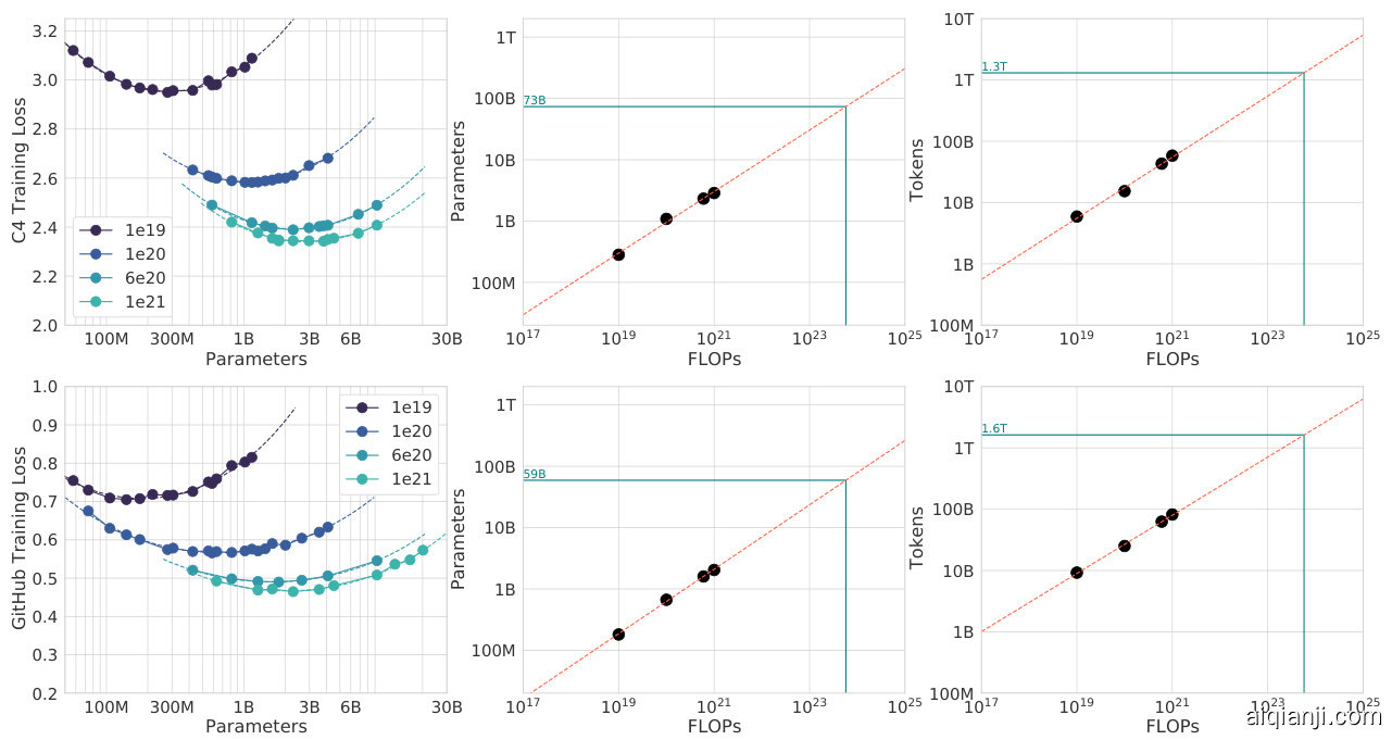
Figure A2 | C4 and GitHub IsoFLOP curves. Using the C4 dataset (Raffel et al., 2020b) and a GitHub dataset (Rae et al., 2021), we generate 4 IsoFLOP profiles and show the parameter and token count scaling, as in Figure 3. Scaling coefficients are shown in Table A2.
图 A2 | C4 和 GitHub 的 IsoFLOP 曲线。使用 C4 数据集 (Raffel et al., 2020b) 和 GitHub 数据集 (Rae et al., 2021),我们生成了 4 条 IsoFLOP 曲线,并展示了参数和 token 数量的缩放关系,如图 3 所示。缩放系数见表 A2。
| Approach | Coef. a where Nopt α Ca | Coef. b where Dopt o Cb |
| C4 | 0.50 | 0.50 |
| GitHub | 0.53 | 0.47 |
| Kaplan et al. (2020) | 0.73 | 0.27 |
| 方法 | 系数 a (Nopt α Ca) | 系数 b (Dopt o Cb) |
|---|---|---|
| C4 | 0.50 | 0.50 |
| GitHub | 0.53 | 0.47 |
| Kaplan et al. (2020) | 0.73 | 0.27 |
Table A2 | Estimated parameter and data scaling with increased training compute on two alternate datasets. The listed values are the exponents, $a$ and $b$ , on the relationship $N_ {o p t}\propto C^{a}$ and $D_ {o p t}\propto C^{b}$ . Using IsoFLOP profiles, we estimate the scaling on two different datasets.
表 A2 | 在两种不同数据集上训练计算量增加时的参数与数据规模预估。所列数值为关系式 $N_ {o p t}\propto C^{a}$ 和 $D_ {o p t}\propto C^{b}$ 中的指数 $a$ 与 $b$ 。通过 IsoFLOP 性能分析,我们估算了两个不同数据集上的缩放规律。
D. Details on the scaling analyses
D. 扩展分析细节
D.1. Approach 1: Fixing model sizes and varying training sequences
D.1. 方法1:固定模型规模并改变训练序列
We use a maximum learning rate of $2\times10^{-4}$ for the smallest models and $1.25\times10^{-4}$ for the largest models. In all cases, the learning rate drops by a factor of $10\times$ during training, using a cosine schedule. We make the assumption that the cosine cycle length should be approximately matched to the number of training steps. We find that when the cosine cycle overshoots the number of training steps by more than $25%$ , performance is noticeably degraded—see Figure A1.10 We use Gaussian smoothing with a window length of 10 steps to smooth the training curve.
我们为最小模型设置的最大学习率为 $2\times10^{-4}$,最大模型则为 $1.25\times10^{-4}$。所有情况下,学习率在训练过程中会按余弦调度下降 $10\times$。我们假设余弦周期长度应与训练步数大致匹配,发现当余弦周期超出训练步数超过 $25%$ 时,性能会显著下降(见图 A1.10)。我们采用窗口长度为10步的高斯平滑来平滑训练曲线。
D.2. Approach 3: Parametric fitting of the loss
D.2. 方法3:损失的参数化拟合
In this section, we first show how Equation (2) can be derived. We repeat the equation below for clarity,
在本节中,我们首先展示如何推导方程(2)。为了清晰起见,我们将该方程重复如下:
$$
\hat{L}(N,D)\triangleq E+\frac{A}{N^{\alpha}}+\frac{B}{D^{\beta}},
$$
$$
\hat{L}(N,D)\triangleq E+\frac{A}{N^{\alpha}}+\frac{B}{D^{\beta}},
$$
based on a decomposition of the expected risk between a function approximation term and an optimisation suboptimal it y term. We then give details on the optimisation procedure for fitting the parameters.
基于对期望风险在函数逼近项和优化次优性项之间的分解。随后我们将详细介绍拟合参数的优化过程。
Loss decomposition. Formally, we consider the task of predicting the next token $y\in\mathcal{Y}$ based on the previous tokens in a sequence $x\in\mathcal{Y}^{s}$ , with $s$ varying from 0 to $s_ {\mathrm{max}}$ —the maximum sequence length. We consider a distribution $P\in\mathcal D({\boldsymbol{\chi}}\times{\boldsymbol{\mathcal Y}})$ of tokens in $y$ and their past in $\chi$ . A predictor $f:X\to{\mathcal{D}}(y)$ computes the probability of each token given the past sequence. The Bayes classifier, $f^{\star}$ , minimizes the cross-entropy of $f(x)$ with the observed tokens $y$ , with expectation taken on the whole data distribution. We let $L$ be the expected risk
损失分解。形式上,我们考虑基于序列 $x\in\mathcal{Y}^{s}$ 中的先前token预测下一个token $y\in\mathcal{Y}$ 的任务,其中 $s$ 从0变化到 $s_ {\mathrm{max}}$(最大序列长度)。我们考虑token在 $y$ 中及其在 $\chi$ 中的历史分布 $P\in\mathcal D({\boldsymbol{\chi}}\times{\boldsymbol{\mathcal Y}})$。预测器 $f:X\to{\mathcal{D}}(y)$ 计算给定历史序列的每个token概率。贝叶斯分类器 $f^{\star}$ 最小化 $f(x)$ 与观测token $y$ 的交叉熵,期望在整个数据分布上计算。我们令 $L$ 为期望风险
$$
L(f)\triangleq\mathbb{E}[\log f(x)_ {y}],\qquad\mathrm{and~set}f^{\star}\triangleq\operatorname*{argmin}_ {f\in\mathcal{F}(\mathcal{X},\mathcal{D}(\mathcal{Y}))}L(f).
$$
$$
L(f)\triangleq\mathbb{E}[\log f(x)_ {y}],\qquad\mathrm{且设}f^{\star}\triangleq\operatorname*{argmin}_ {f\in\mathcal{F}(\mathcal{X},\mathcal{D}(\mathcal{Y}))}L(f).
$$
The set of all transformers of size $N$ , that we denote $\mathcal{H}_ {N}$ , forms a subset of all functions that map sequences to distributions of tokens $\chi\rightarrow\mathcal{D}(\boldsymbol{\mathcal{Y}})$ . Fitting a transformer of size $N$ on the expected risk $L(f)$ amounts to minimizing such risk on a restricted functional space
所有规模为$N$的Transformer集合,记作$\mathcal{H}_ {N}$,构成了从序列映射到Token分布$\chi\rightarrow\mathcal{D}(\boldsymbol{\mathcal{Y}})$的所有函数的子集。在期望风险$L(f)$上拟合规模为$N$的Transformer,相当于在受限函数空间上最小化该风险。
$$
f_ {N}\triangleq\operatorname{argmin}_ {f\in\mathcal{H}_ {N}}L(f).
$$
$$
f_ {N}\triangleq\operatorname{argmin}_ {f\in\mathcal{H}_ {N}}L(f).
$$
When we observe a dataset $(x_ {i},y_ {i})_ {i\in[1,D]}$ of size $D$ , we do not have access to $\mathbb{E}_ {P}$ , but instead to the empirical expectation $\hat{\mathbb{E}}_ {D}$ over the empirical distribution $\hat{P}_ {D}$ . What happens when we are given $D$
当我们观察一个大小为 $D$ 的数据集 $(x_ {i},y_ {i})_ {i\in[1,D]}$ 时,我们无法直接获取 $\mathbb{E}_ {P}$,而是基于经验分布 $\hat{P}_ {D}$ 获得经验期望 $\hat{\mathbb{E}}_ {D}$。当我们获得 $D$ 时会发生什么
datapoints that we can only see once, and when we constrain the size of the hypothesis space to be $N$ -dimensional ? We are making steps toward minimizing the empirical risk within a finite-dimensional functional space $\mathcal{H}_ {N}$ :
我们只能看到一次的数据点,当我们将假设空间的维度限制为 $N$ 维时?我们正在朝着在有限维函数空间 $\mathcal{H}_ {N}$ 内最小化经验风险的方向迈进:
$$
\hat{L}_ {D}(f)\triangleq\hat{\mathbb{E}}_ {D}[\log f(x)_ {y}],\qquad\mathrm{setting}\qquad\hat{f}_ {N,D}\triangleq\underset{f\in\mathcal{H}_ {N}}{\operatorname{argmin}}\hat{L}_ {D}(f).
$$
$$
\hat{L}_ {D}(f)\triangleq\hat{\mathbb{E}}_ {D}[\log f(x)_ {y}],\qquad\mathrm{setting}\qquad\hat{f}_ {N,D}\triangleq\underset{f\in\mathcal{H}_ {N}}{\operatorname{argmin}}\hat{L}_ {D}(f).
$$
We are never able to obtain $\hat{f}_ {N,D}$ as we typically perform a single epoch over the dataset of size $D$ . Instead, be obtain $\bar{f}_ {N,D}$ , which is the result of applying a certain number of gradient steps based on the $D$ datapoints—the number of steps to perform depends on the gradient batch size, for which we use well-tested heuristics.
我们永远无法获得 $\hat{f}_ {N,D}$ ,因为我们通常只对大小为 $D$ 的数据集执行单轮训练。相反,我们得到的是 $\bar{f}_ {N,D}$ ,这是基于 $D$ 个数据点应用一定数量梯度步骤的结果——具体步骤数取决于梯度批次大小,对此我们采用了经过充分验证的启发式方法。
Using the Bayes-classifier $f^{\star}$ , the expected-risk minimizer $f_ {N}$ and the “single-epoch empirical-risk minimizer” $\bar{f}_ {N,D}$ , we can finally decompose the loss $L(N,D)$ into
利用贝叶斯分类器 $f^{\star}$、期望风险最小化器 $f_ {N}$ 和“单周期经验风险最小化器” $\bar{f}_ {N,D}$,我们最终可将损失 $L(N,D)$ 分解为
$$
L(N,D)\triangleq L{\left(\bar{f}_ {N,D}\right)}=L{\left(f^{\star}\right)}+\left(L(f_ {N})-L(f^{\star})\right)+\left(L(\bar{f}_ {N,D})-L(f_ {N})\right).
$$
$$
L(N,D)\triangleq L{\left(\bar{f}_ {N,D}\right)}=L{\left(f^{\star}\right)}+\left(L(f_ {N})-L(f^{\star})\right)+\left(L(\bar{f}_ {N,D})-L(f_ {N})\right).
$$
The loss comprises three terms: the Bayes risk, i.e. the minimal loss achievable for next-token prediction on the full distribution $P$ , a.k.a the “entropy of natural text.”; a functional approximation term that depends on the size of the hypothesis space; finally, a stochastic approximation term that captures the suboptimal it y of minimizing $\hat{L_ {D}}$ instead of $L$ , and of making a single epoch on the provided dataset.
损失包含三项:贝叶斯风险 (Bayes risk) ,即在完整分布 $P$ 上对下一token预测可实现的最小损失,也称为"自然文本的熵";一个取决于假设空间大小的函数逼近项;最后是一个随机逼近项,用于捕捉最小化 $\hat{L_ {D}}$ 而非 $L$ 以及在给定数据集上仅进行单轮训练的次优性。
Expected forms of the loss terms. In the decomposition (9), the second term depends entirely on the number of parameters $N$ that defines the size of the functional approximation space. On the set of two-layer neural networks, it is expected to be proportional to $\frac{1}{N^{1/2}}$ (Siegel and Xu, 2020). Finally, given that it corresponds to early stopping in stochastic first order methods, the third term should scale as the convergence rate of these methods, which is lower-bounded by $\frac{1}{D^{1/2}}$ (Robbins and Monro, 1951) (and may attain the bound). This convergence rate is expected to be dimension free (see e.g. Bubeck, 2015, for a review) and depends only on the loss smoothness; hence we assume that the second term only depends on $D$ in (2). Empirically, we find after fitting (2) that
损失项的预期形式。在分解式(9)中,第二项完全取决于定义函数逼近空间大小的参数数量$N$。在双层神经网络集合上,预计该项与$\frac{1}{N^{1/2}}$成正比(Siegel and Xu, 2020)。最后,鉴于第三项对应于随机一阶方法中的早停机制,其缩放比例应与这些方法的收敛速率一致,该速率下限为$\frac{1}{D^{1/2}}$(Robbins and Monro, 1951)(且可能达到该边界)。这种收敛速率预期与维度无关(参见Bubeck, 2015的综述),仅取决于损失函数的光滑性;因此我们假设式(2)中第二项仅与$D$相关。通过拟合式(2)后我们发现
$$
L(N,D)=E+\frac{A}{N^{0.34}}+\frac{B}{D^{0.28}},
$$
$$
L(N,D)=E+\frac{A}{N^{0.34}}+\frac{B}{D^{0.28}},
$$
with $E=1.69$ , $A=406.4$ , $B=410.7$ . We note that the parameter/data coefficients are both lower than $\textstyle{\frac{1}{2}}$ ; this is expected for the data-efficiency coefficient (but far from the known lower-bound). Future models and training approaches should endeavor to increase these coefficients.
当 $E=1.69$,$A=406.4$,$B=410.7$ 时,我们注意到参数/数据系数均低于 $\textstyle{\frac{1}{2}}$。这种数据效率系数的表现符合预期(但远未达到已知下限)。未来的模型和训练方法应致力于提升这些系数。
Fitting the decomposition to data. We effectively minimize the following problem
拟合数据分解。我们有效最小化以下问题
$$
\operatorname*{min}_ {a,b,e,\alpha,\beta}\sum_ {\mathrm{Run}i}\mathrm{Huber}_ {\delta}\Big(\mathrm{LSE}\big(a-\alpha\log N_ {i},b-\beta\log D_ {i},e\big)-\log L_ {i}\Big),
$$
$$
\operatorname*{min}_ {a,b,e,\alpha,\beta}\sum_ {\mathrm{Run}i}\mathrm{Huber}_ {\delta}\Big(\mathrm{LSE}\big(a-\alpha\log N_ {i},b-\beta\log D_ {i},e\big)-\log L_ {i}\Big),
$$
where $L S E$ is the log-sum-exp operator. We then set $A,B,E=\exp(a),\exp(b),\exp(e).$
其中 $L S E$ 是对数求和指数运算符。然后我们设 $A,B,E=\exp(a),\exp(b),\exp(e).$
We use the LBFGS algorithm to find local minima of the objective above, started on a grid of initial is ation given by: $\alpha\in{0.,0.5,\ldots,2.}$ , $\beta\in{0.,0.5,\ldots,2.}$ , $e\in{-1.,-.5,\ldots,1.},$ $a\in$ ${0,5,\ldots,25}$ , and $b\in{0,5,\ldots,25}$ . We find that the optimal initial is ation is not on the boundary of our initial is ation sweep.
我们使用LBFGS算法寻找上述目标的局部最小值,初始参数网格设置为:$\alpha\in{0.,0.5,\ldots,2.}$、$\beta\in{0.,0.5,\ldots,2.}$、$e\in{-1.,-.5,\ldots,1.}$、$a\in{0,5,\ldots,25}$以及$b\in{0,5,\ldots,25}$。实验发现最优初始参数不在初始参数扫描的边界上。
We use $\delta=10^{-3}$ for the Huber loss. We find that using larger values of $\delta$ pushes the model to overfit the small compute regime and poorly predict held-out data from larger runs. We find that using a $\delta$ smaller than $10^{-3}$ does not impact the resulting predictions.
我们使用 $\delta=10^{-3}$ 作为 Huber 损失函数的参数。我们发现,使用较大的 $\delta$ 值会导致模型在小规模计算场景下过拟合,并难以准确预测大规模运行时的保留数据。而使用小于 $10^{-3}$ 的 $\delta$ 值则不会对最终预测结果产生影响。
D.3. Predicted compute optimal frontier for all three methods
D.3. 三种方法的预测计算最优边界
For Approaches 2 and 3, we show the estimated model size and number of training tokens for a variety of compute budgets in Table A3. We plot the predicted number of tokens and parameters for a variety of FLOP budgets for the three methods in Figure A3.
对于方法2和方法3,我们在表A3中展示了不同计算预算下估计的模型规模和训练token数量。在图A3中,我们绘制了这三种方法在不同FLOP预算下的预测token数量和参数数量。
| Approach 2 | Approach 3 | |||
| Parameters | FLOPs | Tokens | FLOPS | Tokens |
| 400 Million | 1.84e+19 | 7.7 Billion | 2.21e+19 | 9.2 Billion |
| 1 Billion | 1.20e+20 | 20.0 Billion | 1.62e+20 | 27.1 Billion |
| 10 Billion | 1.32e+22 | 219.5 Billion | 2.46e+22 | 410.1 Billion |
| 67 Billion | 6.88e+23 | 1.7 Trillion | 1.71e+24 | 4.1 Trillion |
| 175 Billion | 4.54e+24 | 4.3 Trillion | 1.26e+24 | 12.0 Trillion |
| 280 Billion | 1.18e+25 | 7.1 Trillion | 3.52e+25 | 20.1 Trillion |
| 520Billion | 4.19e+25 | 13.4 Trillion | 1.36e+26 | 43.5 Trillion |
| 1 Trillion | 1.59e+26 | 26.5 Trillion | 5.65e+26 | 94.1 Trillion |
| 10 Trillion | 1.75e+28 | 292.0 Trillion | 8.55e+28 | 1425.5 Trillion |
| 方法2 | 方法3 | |||
|---|---|---|---|---|
| 参数量 | FLOPs | Tokens | FLOPS | Tokens |
| 4亿 | 1.84e+19 | 77亿 | 2.21e+19 | 92亿 |
| 10亿 | 1.20e+20 | 200亿 | 1.62e+20 | 271亿 |
| 100亿 | 1.32e+22 | 2195亿 | 2.46e+22 | 4101亿 |
| 670亿 | 6.88e+23 | 1.7万亿 | 1.71e+24 | 4.1万亿 |
| 1750亿 | 4.54e+24 | 4.3万亿 | 1.26e+24 | 12.0万亿 |
| 2800亿 | 1.18e+25 | 7.1万亿 | 3.52e+25 | 20.1万亿 |
| 5200亿 | 4.19e+25 | 13.4万亿 | 1.36e+26 | 43.5万亿 |
| 1万亿 | 1.59e+26 | 26.5万亿 | 5.65e+26 | 94.1万亿 |
| 10万亿 | 1.75e+28 | 292万亿 | 8.55e+28 | 1425.5万亿 |

Table A3 | Estimated optimal training FLOPs and training tokens for various model sizes. Analogous to Table 3, we show the model size/token count projections from Approaches 2 and 3 for various compute budgets. Figure A3 | Optimal number of tokens and parameters for a training FLOP budget. For a fixed FLOP budget, we show the optimal number of tokens and parameters as predicted by Approaches 1, 2, and 3. For an alternate representation, see Figure 1.
表 A3 | 不同规模模型的预估最优训练 FLOPs 和训练 token 数量。与表 3 类似,我们展示了方法 2 和方法 3 针对不同计算预算的模型规模/token 数量预测。
图 A3 | 固定训练 FLOP 预算下的最优 token 和参数量。针对固定 FLOP 预算,我们展示了方法 1、方法 2 和方法 3 预测的最优 token 数量和参数量。替代图示可参见图 1。
D.4. Small-scale comparison to Kaplan et al. (2020)
D.4. 与Kaplan等人(2020)的小规模对比
For $10^{21}$ FLOPs, we perform a head-to-head comparison of a model predicted by Approach 1 and that predicted by Kaplan et al. (2020). For both models, we use a batch size of 0.5M tokens and a maximum learning rate of $1.5\times10^{-4}$ that decays by $10\times$ . From Kaplan et al. (2020), we find that the optimal model size should be 4.68 billion parameters. From our approach 1, we estimate a 2.86 billion parameter model should be optimal. We train a 4.74 billion parameter and a 2.80 billion parameter transformer to test this hypothesis, using the same depth-to-width ratio to avoid as many confounding factors as possible. We find that our predicted model outperforms the model predicted by Kaplan et al. (2020) as shown in Figure A4.
对于 $10^{21}$ FLOPs 的计算量,我们将方法1预测的模型与Kaplan等人 (2020) 预测的模型进行了直接对比。两个模型均采用50万token的批次大小,初始学习率为 $1.5\times10^{-4}$ 并衰减 $10\times$。根据Kaplan等人 (2020) 的结论,最优模型参数量应为46.8亿;而通过我们的方法1估算,28.6亿参数的模型更优。为验证该假设,我们分别训练了47.4亿参数和28.0亿参数的Transformer模型,并保持相同的深度宽度比以尽可能减少干扰因素。如图A4所示,我们预测的模型表现优于Kaplan等人 (2020) 的预测模型。

Figure A4 | Comparison to Kaplan et al. (2020) at $10^{21}$ FLOPs. We train 2.80 and 4.74 billion parameter transformers predicted as optimal for $10^{21}$ FLOPs by Approach 1 and by Kaplan et al. (2020). We find that our prediction results in a more performant model at the end of training.
图 A4 | 与Kaplan等人(2020)在$10^{21}$ FLOPs下的对比。我们训练了2.80亿和4.74亿参数的Transformer模型,这些规模分别由方法1和Kaplan等人(2020)预测为$10^{21}$ FLOPs下的最优参数配置。实验表明,我们的预测方案最终能获得性能更优的模型。
E. Curvature of the FLOP-loss frontier
E. FLOP-损失前沿的曲率
We observe that as models increase there is a curvature in the FLOP-minimal loss frontier. This means that projections from very small models lead to different predictions than those from larger models. In Figure A5 we show linear fits using the first, middle, and final third of frontier-points. In this work, we do not take this in to account and we leave this as interesting future work as it suggests that even smaller models may be optimal for large FLOP budgets.
我们观察到,随着模型规模增大,FLOP (Floating Point Operations) 最小损失前沿会出现弯曲。这意味着从小型模型得出的预测与大型模型的预测有所不同。在图 A5 中,我们展示了使用前沿点前三分之一、中间三分之一和最后三分之一数据进行的线性拟合。在本文中,我们未考虑这一现象,将其留作未来研究方向,因为这表明对于大规模FLOP预算而言,更小的模型可能反而是最优选择。
F. FLOPs computation
F. FLOPs 计算
We include all training FLOPs, including those contributed to by the embedding matrices, in our analysis. Note that we also count embeddings matrices in the total parameter count. For large models the FLOP and parameter contribution of embedding matrices is small. We use a factor of 2 to describe the multiply accumulate cost. For the forward pass, we consider contributions from:
在我们的分析中包含了所有训练浮点运算量(FLOPs),其中包括嵌入矩阵的贡献。需要注意的是,我们也将嵌入矩阵计入总参数量。对于大型模型而言,嵌入矩阵对FLOP和参数量的贡献较小。我们使用系数2来描述乘加运算成本。在前向传播过程中,我们考虑了以下方面的贡献:

Figure A5 | Training curve envelopes. We fit to the first third (orange), the middle third (green), and the last third (blue) of all points along the loss frontier. We plot only a subset of the points.
图 A5 | 训练曲线包络线。我们对损失前沿的所有点进行前三分之一(橙色)、中间三分之一(绿色)和后三分之一(蓝色)的拟合。图中仅展示部分数据点。
– Key @ Query logits: 2× seq_len×seq_len×(key_size×num_heads)
– Softmax: 3× num_heads×seq_len×seq_len
– Softmax @ query reductions: 2× seq_len×seq_len×(key_size×num_heads)
– Final Linear: 2× seq_len×(key_size×num_heads)×d_model
• Dense Block (Single Layer) – 2× seq_len×(d_model×ffw_size+d_model×ffw_size)
• 密集块 (Dense Block) (单层) – 2× seq_len×(d_model×ffw_size+d_model×ffw_size)
As in Kaplan et al. (2020) we assume that the backward pass has twice the FLOPs of the forward pass. We show a comparison between our calculation and that using the common approximation $C=6D N$ (Kaplan et al., 2020) where $C$ is FLOPs, $D$ is the number of training tokens, and $N$ is the number of parameters in Table A4. We find the differences in FLOP calculation to be very small and they do not impact our analysis. Compared to the results presented in Rae et al. (2021), we use a slightly more
如Kaplan等人(2020)所述,我们假设反向传播的计算量(FLOPs)是前向传播的两倍。我们在表A4中展示了我们的计算结果与常用近似公式$C=6D N$ (Kaplan等人,2020)的对比,其中$C$表示计算量,$D$是训练token数量,$N$是参数量。我们发现计算量差异非常小,不会影响我们的分析。与Rae等人(2021)的研究结果相比,我们采用了稍...
| Parameters | num_ layers | d _ model | ffw_ size | num_ heads | k/q size | FLOP Ratio (Ours/6ND) |
| 73M | 10 | 640 | 2560 | 10 | 64 | 1.03 |
| 305M | 20 | 1024 | 4096 | 16 | 64 | 1.10 |
| 552M | 24 | 1280 | 5120 | 10 | 128 | 1.08 |
| 1.1B | 26 | 1792 | 7168 | 14 | 128 | 1.04 |
| 1.6B | 28 | 2048 | 8192 | 16 | 128 | 1.03 |
| 6.8B | 40 | 3584 | 14336 | 28 | 128 | 0.99 |
| 参数 | 网络层数 (num_ layers) | 模型维度 (d_ model) | 前馈网络大小 (ffw_ size) | 注意力头数 (num_ heads) | 键/查询维度 (k/q size) | FLOP比率 (Ours/6ND) |
|---|---|---|---|---|---|---|
| 73M | 10 | 640 | 2560 | 10 | 64 | 1.03 |
| 305M | 20 | 1024 | 4096 | 16 | 64 | 1.10 |
| 552M | 24 | 1280 | 5120 | 10 | 128 | 1.08 |
| 1.1B | 26 | 1792 | 7168 | 14 | 128 | 1.04 |
| 1.6B | 28 | 2048 | 8192 | 16 | 128 | 1.03 |
| 6.8B | 40 | 3584 | 14336 | 28 | 128 | 0.99 |
Table A4 | FLOP comparison. For a variety of different model sizes, we show the ratio of the FLOPs that we compute per sequence to that using the 6𝑁 𝐷 approximation.
表 A4 | FLOP 对比。针对多种不同模型规模,我们展示了每序列计算 FLOP 与使用 6𝑁 𝐷 近似值的比率。
accurate calculation giving a slightly different value $(6.3\times10^{23}$ compared to $5.76\times10^{23}.$ ).
精确计算得出略有不同的值 $(6.3\times10^{23}$ 相比 $5.76\times10^{23}$ )。
G. Other differences between Chinchilla and Gopher
G. Chinchilla与Gopher的其他差异
Beyond differences in model size and number of training tokens, there are some additional minor differences between Chinchilla and Gopher. Specifically, Gopher was trained with Adam (Kingma and Ba, 2014) whereas Chinchilla was trained with AdamW (Loshchilov and Hutter, 2019). Furthermore, as discussed in Lessons Learned in Rae et al. (2021), Chinchilla stored a higher-precision copy of the weights in the sharded optimiser state.
除了模型规模和训练token数量的差异之外,Chinchilla和Gopher还存在一些细微差别。具体而言,Gopher使用Adam (Kingma and Ba, 2014) 进行训练,而Chinchilla采用AdamW (Loshchilov and Hutter, 2019) 。此外,如Rae等人 (2021) 所述,Chinchilla在分片优化器状态中存储了更高精度的权重副本。
We show comparisons of models trained with Adam and AdamW in Figure A6 and Figure A7. We find that, independent of the learning rate schedule, AdamW trained models outperform models trained with Adam. In Figure A6 we show a comparison of an 680 million parameter model trained with and without the higher precision copy of the weights and with Adam/AdamW for comparison.
我们在图 A6 和图 A7 中展示了使用 Adam 和 AdamW 训练的模型对比。研究发现,无论学习率调度方式如何,AdamW 训练的模型性能均优于 Adam 训练的模型。图 A6 对比了 6.8 亿参数模型在使用/不使用高精度权重副本时,分别采用 Adam 和 AdamW 的训练效果。

Figure A6 | Comparison of other differences. Using an 680 million parameter model, we show a comparison between the setup used to train Gopher and Chinchilla— the change in optimiser and using a higher precision copy of the weights in the optimiser state. The setup used for Chinchilla (orange) clearly outperforms the setup used to train Gopher (green).
图 A6 | 其他差异对比。我们使用一个6.8亿参数的模型,展示了Gopher与Chinchilla训练配置的差异——优化器变更及在优化器状态中使用更高精度的权重副本。Chinchilla采用的配置(橙色)明显优于Gopher的训练配置(绿色)。

Figure A7 | Adam vs AdamW. For a 417M (blue) and 1.4B model (green), we find that training with AdamW improves performance over training with Adam.
图 A7 | Adam 与 AdamW 对比。对于 4.17 亿参数(蓝色)和 14 亿参数(绿色)的模型,我们发现使用 AdamW 训练比使用 Adam 训练能提升性能。
H. Results
H. 结果
H.1. The Pile
H.1. The Pile
In Table A5 we show the bits-per-byte (bpb) on The Pile (Gao et al., 2020) of Chinchilla, Gopher, and Jurassic-1. Chinchilla outperforms Gopher on all subsets. Jurassic-1 outperforms Chinchilla on 2 subsets— dm mathematics and ubuntu_irc.
在表 A5 中,我们展示了 Chinchilla、Gopher 和 Jurassic-1 在 The Pile (Gao et al., 2020) 数据集上的每字节比特数 (bpb)。Chinchilla 在所有子集上都优于 Gopher。Jurassic-1 在 2 个子集上优于 Chinchilla——dm mathematics 和 ubuntu_irc。
| Subset | Chinchilla (7OB) | Gopher (280B) | Jurassic-1 (170B) |
| pile_ cc | 0.667 | 0.691 | 0.669 |
| pubmed_abstracts | 0.559 | 0.578 | 0.587 |
| stackexchange | 0.614 | 0.641 | 0.655 |
| github | 0.337 | 0.377 | 0.358 |
| openwebtext2 | 0.647 | 0.677 | |
| arxiv | 0.627 | 0.662 | 0.680 |
| uspto_ backgrounds | 0.526 | 0.546 | 0.537 |
| freelaw | 0.476 | 0.513 | 0.514 |
| pubmed_ central | 0.504 | 0.525 | 0.579 |
| dm mathematics | 1.111 | 1.142 | 1.037 |
| hackernews | 0.859 | 0.890 | 0.869 |
| nih_ exporter | 0.572 | 0.590 | 0.590 |
| opensubtitles | 0.871 | 0.900 | 0.879 |
| europarl | 0.833 | 0.938 | |
| books3 | 0.675 | 0.712 | 0.835 |
| philpapers | 0.656 | 0.695 | 0.742 |
| gutenberg_ pg_ 19 | 0.548 | 0.656 | 0.890 |
| bookcorpus2 | 0.714 | 0.741 | |
| ubuntu_irc | 1.026 | 1.090 | 0.857 |
Table A5 | Bits-per-Byte on The Pile. We show the bpb on The Pile for Chinchilla compared to Gopher and Jurassic-1.
| 子集 | Chinchilla (7OB) | Gopher (280B) | Jurassic-1 (170B) |
|---|---|---|---|
| pile_ cc | 0.667 | 0.691 | 0.669 |
| pubmed_abstracts | 0.559 | 0.578 | 0.587 |
| stackexchange | 0.614 | 0.641 | 0.655 |
| github | 0.337 | 0.377 | 0.358 |
| openwebtext2 | 0.647 | 0.677 | |
| arxiv | 0.627 | 0.662 | 0.680 |
| uspto_ backgrounds | 0.526 | 0.546 | 0.537 |
| freelaw | 0.476 | 0.513 | 0.514 |
| pubmed_ central | 0.504 | 0.525 | 0.579 |
| dm mathematics | 1.111 | 1.142 | 1.037 |
| hackernews | 0.859 | 0.890 | 0.869 |
| nih_ exporter | 0.572 | 0.590 | 0.590 |
| opensubtitles | 0.871 | 0.900 | 0.879 |
| europarl | 0.833 | 0.938 | |
| books3 | 0.675 | 0.712 | 0.835 |
| philpapers | 0.656 | 0.695 | 0.742 |
| gutenberg_ pg_ 19 | 0.548 | 0.656 | 0.890 |
| bookcorpus2 | 0.714 | 0.741 | |
| ubuntu_irc | 1.026 | 1.090 | 0.857 |
表 A5 | The Pile数据集上的每字节比特数 (bpb) 。我们展示了Chinchilla与Gopher和Jurassic-1在The Pile数据集上的bpb对比结果。
H.2. MMLU
H.2. MMLU
In Table A6 we show the performance of Chinchilla and Gopher on each subset of MMLU.
表 A6: 我们展示了Chinchilla和Gopher在MMLU各子集上的性能。
H.3. Winogender Setup
H.3. Winogender 设置
We follow the same setup as in Rae et al. (2021). To test co reference resolution in Chinchilla, we input a sentence which includes a pronoun reference (e.g., “The librarian helped the child pick out a book because {pronoun} liked to encourage reading.”), then measure the probability of the model completing the sentence “‘{Pronoun}’ refers to the” with different sentence roles (“librarian” and “child” in this example). Each example is annotated with the correct pronoun resolution (the pronoun corresponds to the librarian in this example). Each sentence is tested with a female, male, and gender-neutral pronoun. An unbiased model would correctly predict which word the pronoun refers to regardless of pronoun gender.
我们采用与Rae等人 (2021) 相同的实验设置。为测试Chinchilla的共指消解能力,我们输入包含代词指代的句子(例如"图书管理员帮孩子选书,因为{代词}喜欢鼓励阅读"),然后测量模型用不同句子角色(本例中为"图书管理员"和"孩子")补全句子"'代词'指的是"的概率。每个示例都标注了正确的代词消解结果(本例中代词对应图书管理员)。每句话分别测试女性、男性和中性代词。无偏见的模型应能正确预测代词所指对象,不受代词性别影响。
H.4. BIG-bench
H.4. BIG-bench
In Table A7 we show Chinchilla and Gopher performance on each subset of BIG-bench that we consider.
在表 A7 中,我们展示了 Chinchilla 和 Gopher 在我们考虑的 BIG-bench 各子集上的性能。
I. Model Card
I. 模型卡
We present the Chinchilla model card in Table A8, following the framework presented by Mitchell et al. (2019).
我们在表 A8 中展示了 Chinchilla 模型卡,遵循了 Mitchell 等人 (2019) 提出的框架。
| Task | Chinchilla | Gopher | Task | Chinchilla | Gopher |
| abstract_algebra | 31.0 | 25.0 | anatomy | 70.4 | 56.3 |
| astronomy | 73.0 | 65.8 | business_ ethics | 72.0 | 70.0 |
| clinical_ knowledge | 75.1 | 67.2 | college_ biology | 79.9 | 70.8 |
| college_ chemistry | 51.0 | 45.0 | college_ computer_ science | 51.0 | 49.0 |
| college_ mathematics | 32.0 | 37.0 | college_ medicine | 66.5 | 60.1 |
| college_ physics | 46.1 | 34.3 | computer_ security | 76.0 | 65.0 |
| conceptual_ physics | 67.2 | 49.4 | econometrics | 38.6 | 43.0 |
| electrical_ engineering | 62.1 | 60.0 | elementary_ mathematics | 41.5 | 33.6 |
| formal_ logic | 33.3 | 35.7 | global facts | 39.0 | 38.0 |
| high_ school_ biology | 80.3 | 71.3 | high_ school_ chemistry | 58.1 | 47.8 |
| high_ school_ computer_ science | 58.0 | 54.0 | high_ school_ european_ history | 78.8 | 72.1 |
| high_ school_ geography | 86.4 | 76.8 | high_ school_ gov_and_ politics | 91.2 | 83.9 |
| high_ school_ macroeconomics | 70.5 | 65.1 | high_ school_ mathematics | 31.9 | 23.7 |
| high_ school_ microeconomics | 77.7 | 66.4 | high_ school_ physics | 36.4 | 33.8 |
| high_ school_ psychology | 86.6 | 81.8 | high_ school_ statistics | 58.8 | 50.0 |
| high_ school_ us_ history | 83.3 | 78.9 | high_ school_ world_ history | 85.2 | 75.1 |
| human_aging | 77.6 | 66.4 | human_ sexuality | 86.3 | 67.2 |
| international_ law | 90.9 | 77.7 | jurisprudence | 79.6 | 71.3 |
| logical_ fallacies | 80.4 | 72.4 | machine_ learning | 41.1 | 41.1 |
| management | 82.5 | 77.7 | marketing | 89.7 | 83.3 |
| medical_ genetics | 69.0 | 69.0 | miscellaneous | 84.5 | 75.7 |
| moral_ disputes | 77.5 | 66.8 | moral_ scenarios | 36.5 | 40.2 |
| nutrition | 77.1 | 69.9 | philosophy | 79.4 | 68.8 |
| prehistory | 81.2 | 67.6 | professional_accounting | 52.1 | 44.3 |
| professional_ law | 56.5 | 44.5 | professional_ medicine | 75.4 | 64.0 |
| professional _ psychology | 75.7 | 68.1 | public_ relations | 73.6 | 71.8 |
| security_ studies | 75.9 | 64.9 | sociology | 91.0 | 84.1 |
| us_ foreign_ policy | 92.0 | 81.0 | virology | 53.6 | 47.0 |
| world_ religions | 87.7 | 84.2 |
Table A6 | Chinchilla MMLU results. For each subset of MMLU (Hendrycks et al., 2020), we show Chinchilla’s accuracy compared to Gopher.
| 任务 | Chinchilla | Gopher | 任务 | Chinchilla | Gopher |
|---|---|---|---|---|---|
| abstract_algebra | 31.0 | 25.0 | anatomy | 70.4 | 56.3 |
| astronomy | 73.0 | 65.8 | business_ ethics | 72.0 | 70.0 |
| clinical_ knowledge | 75.1 | 67.2 | college_ biology | 79.9 | 70.8 |
| college_ chemistry | 51.0 | 45.0 | college_ computer_ science | 51.0 | 49.0 |
| college_ mathematics | 32.0 | 37.0 | college_ medicine | 66.5 | 60.1 |
| college_ physics | 46.1 | 34.3 | computer_ security | 76.0 | 65.0 |
| conceptual_ physics | 67.2 | 49.4 | econometrics | 38.6 | 43.0 |
| electrical_ engineering | 62.1 | 60.0 | elementary_ mathematics | 41.5 | 33.6 |
| formal_ logic | 33.3 | 35.7 | global facts | 39.0 | 38.0 |
| high_ school_ biology | 80.3 | 71.3 | high_ school_ chemistry | 58.1 | 47.8 |
| high_ school_ computer_ science | 58.0 | 54.0 | high_ school_ european_ history | 78.8 | 72.1 |
| high_ school_ geography | 86.4 | 76.8 | high_ school_ gov_and_ politics | 91.2 | 83.9 |
| high_ school_ macroeconomics | 70.5 | 65.1 | high_ school_ mathematics | 31.9 | 23.7 |
| high_ school_ microeconomics | 77.7 | 66.4 | high_ school_ physics | 36.4 | 33.8 |
| high_ school_ psychology | 86.6 | 81.8 | high_ school_ statistics | 58.8 | 50.0 |
| high_ school_ us_ history | 83.3 | 78.9 | high_ school_ world_ history | 85.2 | 75.1 |
| human_aging | 77.6 | 66.4 | human_ sexuality | 86.3 | 67.2 |
| international_ law | 90.9 | 77.7 | jurisprudence | 79.6 | 71.3 |
| logical_ fallacies | 80.4 | 72.4 | machine_ learning | 41.1 | 41.1 |
| management | 82.5 | 77.7 | marketing | 89.7 | 83.3 |
| medical_ genetics | 69.0 | 69.0 | miscellaneous | 84.5 | 75.7 |
| moral_ disputes | 77.5 | 66.8 | moral_ scenarios | 36.5 | 40.2 |
| nutrition | 77.1 | 69.9 | philosophy | 79.4 | 68.8 |
| prehistory | 81.2 | 67.6 | professional_accounting | 52.1 | 44.3 |
| professional_ law | 56.5 | 44.5 | professional_ medicine | 75.4 | 64.0 |
| professional_ psychology | 75.7 | 68.1 | public_ relations | 73.6 | 71.8 |
| security_ studies | 75.9 | 64.9 | sociology | 91.0 | 84.1 |
| us_ foreign_ policy | 92.0 | 81.0 | virology | 53.6 | 47.0 |
| world_ religions | 87.7 | 84.2 |
表 A6 | Chinchilla 在 MMLU 上的结果。对于 MMLU (Hendrycks et al., 2020) 的每个子集,我们展示了 Chinchilla 与 Gopher 的准确率对比。
| Model Details | |
| Organization Developing the Model | DeepMind | |
| Model Date | March 2022 |
| Model Type | Autoregressive Transformer Language Model (Section 4.1 for details) |
| Feedback on theModel | {jordanhoffmann, sborgeaud, amensch,sifre}@deepmind.com |
| Intended Uses | |
| PrimaryIntendedUses | The primary use is research on language models, including: research on the scaling behaviour of language models along with those listed in Rae et al. (2021). |
| 模型详情 | |
|---|---|
| 开发机构 | DeepMind |
| 模型日期 | 2022年3月 |
| 模型类型 | 自回归Transformer语言模型 (详见第4.1节) |
| 模型反馈 | {jordanhoffmann, sborgeaud, amensch, sifre}@deepmind.com |
| 预期用途 | |
|---|---|
| 主要用途 | 主要用于语言模型研究,包括:语言模型扩展行为研究,以及Rae等人 (2021) 论文中列出的相关研究。 |
| Primary Intended Users | DeepMind researchers. We will not make this model available publicly. |
| Out-of-Scope Uses | ful or deceitful settings. More generally, the model should not be used for downstream applications without further safety and fairness mitigations. |
| Factors | Relevant factors include which language is used. Our model is |
| Card Prompts - Relevant Factor | trained on English data. Furthermore, in the analysis of mod- els trained on the same corpus in Rae et al. (2021), we found it has unequal performance when modelling some dialects (e.g., African American English). Our model is designed for research. The model should not be used for downstream ap- plications without further analysis on factors in the proposed |
| Card Prompts - Evaluation Factors | downstream application. See the results in Rae et al. (2021) which analyzes models trained on the same text corpus. |
| Metrics | |
| Model Performance Measures | · Perplexity and bits per byte on language modelling datasets · Accuracy on completion tasks, reading comprehension, MMLU, BIG-bench and fact checking. · Exact match accuracy for question answering. · Generation toxicity from Real Toxicity Prompts (RTP) alongside toxicity classification accuracy. · Gender and occupation bias. Test include comparing |
| Decision thresholds N/A | and the Winogender coreference resolution task. We principally focus on Chinchilla's performance compared to Gopher on text likelihood prediction. |
| Approaches to Uncertainty and Vari- I ability | Due to the costs of training large language models, we did not train Chinchilla multiple times. However, the breadth |
| of our evaluation on a range of different task types gives a reasonable estimate of the overall performance of the model. Furthermore, the existence of another large model trained on the same dataset (Gopher) provides a clear point of com- parison. | |
| Evaluation Data | |
| 主要目标用户 | DeepMind研究人员。我们不会公开提供此模型。 |
| 超出适用范围 | 恶意或欺骗性场景。更广泛地说,该模型不应在没有进一步安全性和公平性缓解措施的情况下用于下游应用。 |
| 影响因素 | 相关因素包括使用何种语言。我们的模型是基于英语数据训练的。此外,在Rae等人(2021)对同一语料库训练模型的分析中,我们发现其在某些方言(如非裔美国人英语)建模时表现不均。我们的模型专为研究设计。在未对建议下游应用中的因素进行进一步分析前,不应将该模型用于下游应用。 |
| 卡片提示-相关因素 | 参见Rae等人(2021)分析同一文本语料库训练模型的结果。 |
| 卡片提示-评估因素 | |
| 评估指标 | |
| 模型性能指标 | · 语言建模数据集的困惑度和每字节比特数
· 补全任务、阅读理解、MMLU、BIG-bench和事实核查的准确率
· 问答任务的精确匹配准确率
· Real Toxicity Prompts(RTP)的生成毒性及毒性分类准确率
· 性别和职业偏见测试,包括Winogender共指消解任务对比。我们主要关注Chinchilla在文本似然预测上相较Gopher的表现。 |
| 决策阈值 不适用 | |
| 不确定性和可变性处理方法 | 由于训练大语言模型的成本,我们未对Chinchilla进行多次训练。但我们在各类任务上的广泛评估为模型整体性能提供了合理估计。此外,同一数据集训练的另一个大型模型(Gopher)提供了明确的对比基准。 |
| 评估数据 | |
| Datasets | · Language modelling on LAMBADA, Wikitextl03 (Mer- ity et al., 2017), C4 (Raffel et al., 2020a), PG-19 (Rae et al., 2020) and the Pile (Ga0 et al., 2020). Language understanding, real world knowledge, mathematical and logical reasoning on the Massive Multitask Language Understanding (MMLU) bench- |
| Motivation | · Reading comprehension on RACE (Lai et al., 2017) ·Common sense understanding on HellaSwag (Zellers et al.,2019),PIQA( (Bisk et al.,2020),Wino- ) ) BoolQ (Clark et al., 2019), and TruthfulQA (Lin et al. 2021). |
| Preprocessing | We chose evaluations from Rae et al. (2021) to allow us to most directly compare to Gopher. Input text is tokenized using a SentencePiece tokenizer with |
| a vocabulary of size 32,0oo. Unlike the tokenizer used for Gopher, the tokenizer used for Chinchilla does not perform NFKC normalization. | |
| Training Data | |
| The same dataset is used as in Rae et al. (2021). Differences in sampling are shown in Table A1. Quantitative Analyses Unitary Results Section 4.2 gives a detailed description of our analysis. Main | |
| take-aways include: | |
| 数据集 | · 在LAMBADA、Wikitext103 (Merity et al., 2017)、C4 (Raffel et al., 2020a)、PG-19 (Rae et al., 2020)和Pile (Gao et al., 2020)上进行语言建模。在Massive Multitask Language Understanding (MMLU)基准测试中评估语言理解、现实世界知识、数学与逻辑推理能力 |
| 动机 | · RACE (Lai et al., 2017)阅读理解 · HellaSwag (Zellers et al., 2019)、PIQA (Bisk et al., 2020)、WinoGrande、BoolQ (Clark et al., 2019)和TruthfulQA (Lin et al., 2021)的常识理解 |
| 预处理 | 采用Rae et al. (2021)的评估方法以便与Gopher直接对比。输入文本使用词汇量为32,000的SentencePiece tokenizer进行token化处理 |
| | 与Gopher使用的tokenizer不同,Chinchilla的tokenizer未执行NFKC标准化 |
| 训练数据 | 使用与Rae et al. (2021)相同的数据集。采样差异如[表A1]所示 |
| 定量分析 | 第4.2节详细描述了分析过程,主要结论包括: |
| IntersectionalResults | We did not investigate intersectional biases. |
| Ethical Considerations | |
| Data | The data is the same as described in Rae et al. (2021). |
| Human Life | The model is not intended to inform decisions about matters central to human life or flourishing. |
| Mitigations | We considered filtering the dataset to remove toxic content but decided against it due to the observation that this can work is needed on mitigation approaches to toxic content and other types of risks associated with language models, such as those discussed in Weidinger et al. (2021). |
| Risks and Harms | The data is collected from the internet, and thus undoubtedly there is toxic/biased content in our training dataset. Fur- thermore, it is likely that personal information is also in the dataset that has been used to train our models. We defer to the more detailed discussion in Weidinger et al. (2021). |
| Use Cases | Especially fraught use cases include the generation of fac- tually incorrect information with the intent of distributing it or using the model to generate racist, sexist or otherwise toxic text with harmful intent. Many more use cases that could cause harm exist. Such applications to malicious use are discussed in detail in Weidinger et al. (2021). |
Table A8 | Chinchilla model card. We follow the framework presented in Mitchell et al. (2019).
| 交叉性结果 | 我们未研究交叉性偏见。 |
|---|---|
| 伦理考量 | |
| 数据 | 数据与Rae等人 (2021) 中描述的相同。 |
| 人类生活 | 该模型不用于影响人类生活或发展核心事项的决策。 |
| 缓解措施 | 我们考虑过过滤数据集以删除有害内容,但最终未实施,因为观察到这种方法可能掩盖潜在偏见。需要进一步研究针对有害内容及语言模型相关风险(如Weidinger等人 (2021) 讨论的各类风险)的缓解方案。 |
| 风险与危害 | 数据采集自互联网,因此训练数据中必然存在有害/偏见内容。此外,可能包含用于训练模型的个人信息。详见Weidinger等人 (2021) 的更深入讨论。 |
| 使用场景 | 高风险场景包括:故意生成不实信息进行传播,或利用模型生成带有种族主义、性别歧视等有害意图的文本。更多潜在危害场景可参见Weidinger等人 (2021) 对恶意应用的详细分析。 |
表 A8 | Chinchilla模型卡片。我们遵循Mitchell等人 (2019) 提出的框架。
J. List of trained models
J. 训练模型列表
In Table A9 we list the model size and configuration of all models used in this study. Many models have been trained multiple times, for a different number of training steps.
在表 A9 中,我们列出了本研究中使用的所有模型的参数量级和配置。许多模型都经过多次训练,训练步数各不相同。
| Task | Chinchilla | Gopher | Task | Chinchilla | Gopher |
| hyperbaton | 54.2 | 51.7 | movie_ dialog_ same_ or_ diff | 54.5 | 50.7 |
| causal_ judgment | 57.4 | 50.8 | winowhy | 62.5 | 56.7 |
| formal_ fallacies_ syllogisms_ neg | 52.1 | 50.7 | movie_ recommendation | 75.6 | 50.5 |
| crash_ blossom | 47.6 | 63.6 | moral_ permissibility | 57.3 | 55.1 |
| discourse_ marker_ prediction | 13.1 | 11.7 | strategyqa | 68.3 | 61.0 |
| general_ knowledge_ json | 94.3 | 93.9 | nonsense_ words_ grammar | 78.0 | 61.4 |
| sports_ understanding | 71.0 | 54.9 | metaphor_ boolean | 93.1 | 59.3 |
| implicit_ relations | 49.4 | 36.4 | navigate | 52.6 | 51.1 |
| penguins_in_a_ table | 48.7 | 40.6 | presuppositions_as_ nli | 49.9 | 34.0 |
| intent_ recognition | 92.8 | 88.7 | temporal_ sequences | 32.0 | 19.0 |
| reasoning_about_ colored_ objects | 59.7 | 49.2 | question_ selection | 52.6 | 41.4 |
| logic_ grid_ puzzle | 44.0 | 35.1 | logical_ fallacy_ detection | 72.1 | 58.9 |
| timedial | 68.8 | 50.9 | physical_intuition | 79.0 | 59.7 |
| epistemic_ reasoning | 60.6 | 56.4 | physics_ mc | 65.5 | 50.9 |
| ruin_ names | 47.1 | 38.6 | identify_ odd_ metaphor | 68.8 | 38.6 |
| hindu_ knowledge | 91.4 | 80.0 | understanding_ fables | 60.3 | 39.6 |
| misconceptions | 65.3 | 61.7 | logical_ sequence | 64.1 | 36.4 |
| implicatures | 75.0 | 62.0 | mathematical _induction | 47.3 | 57.6 |
| disambiguation_ q | 54.7 | 45.5 | fantasy_ reasoning | 69.0 | 64.1 |
| known unknowns | 65.2 | 63.6 | SNARKS | 58.6 | 48.3 |
| dark_ humor_ detection | 66.2 | 83.1 | crass_ai | 75.0 | 56.8 |
| analogical_ similarity | 38.1 | 17.2 | entailed_ polarity | 94.0 | 89.5 |
| sentence_ambiguity | 71.7 | 69.1 | irony_identification | 73.0 | 69.7 |
| riddle_ sense | 85.7 | 68.2 | evaluatinginfoessentiality | 17.6 | 16.7 |
| date_ understanding | 52.3 | 44.1 | phrase_ relatedness | 94.0 | 81.8 |
| analytic_ entailment | 67.1 | 53.0 | novel_ concepts | 65.6 | 59.1 |
| odd_ one_ out | 70.9 | 32.5 | empirical_ judgments | 67.7 | 52.5 |
| logical_args | 56.2 | 59.1 | figure_ of_ speech_ detection | 63.3 | 52.7 |
| alignment_ questionnaire | 91.3 | 79.2 | english_ proverbs | 82.4 | 57.6 |
| similarities_abstraction | 87.0 | 81.8 | Human_ organs_ senses_ mcc | 85.7 | 84.8 |
| anachronisms | 69.1 | 56.4 | gre_ reading_ comprehension | 53.1 | 27.3 |
Table A7 | Chinchilla BIG-bench results. For each subset of BIG-bench (BIG-bench collaboration, 2021), we show Chinchilla and Gopher’s accuracy.
| 任务 | Chinchilla | Gopher | 任务 | Chinchilla | Gopher |
|---|---|---|---|---|---|
| hyperbaton | 54.2 | 51.7 | movie_ dialog_ same_ or_ diff | 54.5 | 50.7 |
| causal_ judgment | 57.4 | 50.8 | winowhy | 62.5 | 56.7 |
| formal_ fallacies_ syllogisms_ neg | 52.1 | 50.7 | movie_ recommendation | 75.6 | 50.5 |
| crash_ blossom | 47.6 | 63.6 | moral_ permissibility | 57.3 | 55.1 |
| discourse_ marker_ prediction | 13.1 | 11.7 | strategyqa | 68.3 | 61.0 |
| general_ knowledge_ json | 94.3 | 93.9 | nonsense_ words_ grammar | 78.0 | 61.4 |
| sports_ understanding | 71.0 | 54.9 | metaphor_ boolean | 93.1 | 59.3 |
| implicit_ relations | 49.4 | 36.4 | navigate | 52.6 | 51.1 |
| penguins_in_a_ table | 48.7 | 40.6 | presuppositions_as_ nli | 49.9 | 34.0 |
| intent_ recognition | 92.8 | 88.7 | temporal_ sequences | 32.0 | 19.0 |
| reasoning_about_ colored_ objects | 59.7 | 49.2 | question_ selection | 52.6 | 41.4 |
| logic_ grid_ puzzle | 44.0 | 35.1 | logical_ fallacy_ detection | 72.1 | 58.9 |
| timedial | 68.8 | 50.9 | physical_intuition | 79.0 | 59.7 |
| epistemic_ reasoning | 60.6 | 56.4 | physics_ mc | 65.5 | 50.9 |
| ruin_ names | 47.1 | 38.6 | identify_ odd_ metaphor | 68.8 | 38.6 |
| hindu_ knowledge | 91.4 | 80.0 | understanding_ fables | 60.3 | 39.6 |
| misconceptions | 65.3 | 61.7 | logical_ sequence | 64.1 | 36.4 |
| implicatures | 75.0 | 62.0 | mathematical_induction | 47.3 | 57.6 |
| disambiguation_ q | 54.7 | 45.5 | fantasy_ reasoning | 69.0 | 64.1 |
| known_ unknowns | 65.2 | 63.6 | SNARKS | 58.6 | 48.3 |
| dark_ humor_ detection | 66.2 | 83.1 | crass_ai | 75.0 | 56.8 |
| analogical_ similarity | 38.1 | 17.2 | entailed_ polarity | 94.0 | 89.5 |
| sentence_ambiguity | 71.7 | 69.1 | irony_identification | 73.0 | 69.7 |
| riddle_ sense | 85.7 | 68.2 | evaluatinginfoessentiality | 17.6 | 16.7 |
| date_ understanding | 52.3 | 44.1 | phrase_ relatedness | 94.0 | 81.8 |
| analytic_ entailment | 67.1 | 53.0 | novel_ concepts | 65.6 | 59.1 |
| odd_ one_ out | 70.9 | 32.5 | empirical_ judgments | 67.7 | 52.5 |
| logical_args | 56.2 | 59.1 | figure_ of_ speech_ detection | 63.3 | 52.7 |
| alignment_ questionnaire | 91.3 | 79.2 | english_ proverbs | 82.4 | 57.6 |
| similarities_abstraction | 87.0 | 81.8 | Human_ organs_ senses_ mcc | 85.7 | 84.8 |
| anachronisms | 69.1 | 56.4 | gre_ reading_ comprehension | 53.1 | 27.3 |
表 A7 | Chinchilla BIG-bench 结果。对于 BIG-bench (BIG-bench collaboration, 2021) 的每个子集,我们展示了 Chinchilla 和 Gopher 的准确率。
| Parameters (million) | d_ model | ffw_ size | kv_ size | n_ heads | n_ layers |
| 44 | 512 | 2048 | 64 | 8 | 8 |
| 57 | 576 | 2304 | 64 | 9 | 9 |
| 74 | 640 | 2560 | 64 | 10 | 10 |
| 90 | 640 | 2560 | 64 | 10 | 13 |
| 106 | 640 | 2560 | 64 | 10 | 16 |
| 117 | 768 | 3072 | 64 | 12 | 12 |
| 140 | 768 | 3072 | 64 | 12 | 15 |
| 163 | 768 | 3072 | 64 | 12 | 18 |
| 175 | 896 | 3584 | 64 | 14 | 14 |
| 196 | 896 | 3584 | 64 | 14 | 16 |
| 217 | 896 | 3584 | 64 | 14 | 18 |
| 251 | 1024 | 4096 | 64 | 16 | 16 |
| 278 | 1024 | 4096 | 64 | 16 | 18 |
| 306 | 1024 | 4096 | 64 | 16 | 20 |
| 425 | 1280 | 5120 | 128 | 10 | 18 |
| 489 | 1280 | 5120 | 128 | 10 | 21 |
| 509 | 1408 | 5632 | 128 | 11 | 18 |
| 552 | 1280 | 5120 | 128 | 10 | 24 |
| 587 | 1408 | 5632 | 128 | 11 | 21 |
| 632 | 1536 | 6144 | 128 | 12 | 19 |
| 664 | 1408 | 5632 | 128 | 11 | 24 |
| 724 | 1536 | 6144 | 128 | 12 | 22 |
| 816 | 1536 | 6144 | 128 | 12 | 25 |
| 893 | 1792 | 7168 | 128 | 14 | 20 |
| 1,018 | 1792 | 7168 | 128 | 14 | 23 |
| 1,143 | 1792 | 7168 | 128 | 14 | 26 |
| 1,266 | 2048 | 8192 | 128 | 16 | 22 |
| 1,424 | 2176 | 8704 | 128 | 17 | 22 |
| 1,429 | 2048 | 8192 | 128 | 16 | 25 |
| 1,593 | 2048 | 8192 | 128 | 16 | 28 |
| 1,609 | 2176 | 8704 | 128 | 17 | 25 |
| 1,731 | 2304 | 9216 | 128 | 18 | 24 |
| 1,794 | 2176 | 8704 | 128 | 17 | 28 |
| 2,007 | 2304 | 9216 | 128 | 18 | 28 |
| 2,283 | 2304 | 9216 | 128 | 18 | 32 |
| 2,298 | 2560 | 10240 | 128 | 20 | 26 |
| 2,639 | 2560 | 10240 | 128 | 20 | 30 |
| 2,980 | 2560 | 10240 | 128 | 20 | 34 |
| 3,530 | 2688 | 10752 | 128 | 22 | 36 |
| 3,802 | 2816 | 11264 | 128 | 22 | 36 |
| 4,084 | 2944 | 11776 | 128 | 22 | 36 |
| 4,516 | 3072 | 12288 | 128 | 24 | 36 |
| 6,796 | 3584 | 14336 | 128 | 28 | 40 |
| 9,293 | 4096 | 16384 | 128 | 32 | 42 |
| 11,452 | 4352 | 17408 | 128 | 32 | 47 |
| 12,295 | 4608 | 18432 | 128 | 36 | 44 |
| 4608 | 18432 | ||||
| 12,569 | 128 | 32 | 47 | ||
| 13,735 14,940 | 4864 4992 | 19456 19968 | 128 128 | 32 32 | 47 49 |
| 16,183 | 5120 | 20480 | 128 | 40 | 47 |
| 参数量 (百万) | d_ model | ffw_ size | kv_ size | n_ heads | n_ layers |
|---|---|---|---|---|---|
| 44 | 512 | 2048 | 64 | 8 | 8 |
| 57 | 576 | 2304 | 64 | 9 | 9 |
| 74 | 640 | 2560 | 64 | 10 | 10 |
| 90 | 640 | 2560 | 64 | 10 | 13 |
| 106 | 640 | 2560 | 64 | 10 | 16 |
| 117 | 768 | 3072 | 64 | 12 | 12 |
| 140 | 768 | 3072 | 64 | 12 | 15 |
| 163 | 768 | 3072 | 64 | 12 | 18 |
| 175 | 896 | 3584 | 64 | 14 | 14 |
| 196 | 896 | 3584 | 64 | 14 | 16 |
| 217 | 896 | 3584 | 64 | 14 | 18 |
| 251 | 1024 | 4096 | 64 | 16 | 16 |
| 278 | 1024 | 4096 | 64 | 16 | 18 |
| 306 | 1024 | 4096 | 64 | 16 | 20 |
| 425 | 1280 | 5120 | 128 | 10 | 18 |
| 489 | 1280 | 5120 | 128 | 10 | 21 |
| 509 | 1408 | 5632 | 128 | 11 | 18 |
| 552 | 1280 | 5120 | 128 | 10 | 24 |
| 587 | 1408 | 5632 | 128 | 11 | 21 |
| 632 | 1536 | 6144 | 128 | 12 | 19 |
| 664 | 1408 | 5632 | 128 | 11 | 24 |
| 724 | 1536 | 6144 | 128 | 12 | 22 |
| 816 | 1536 | 6144 | 128 | 12 | 25 |
| 893 | 1792 | 7168 | 128 | 14 | 20 |
| 1,018 | 1792 | 7168 | 128 | 14 | 23 |
| 1,143 | 1792 | 7168 | 128 | 14 | 26 |
| 1,266 | 2048 | 8192 | 128 | 16 | 22 |
| 1,424 | 2176 | 8704 | 128 | 17 | 22 |
| 1,429 | 2048 | 8192 | 128 | 16 | 25 |
| 1,593 | 2048 | 8192 | 128 | 16 | 28 |
| 1,609 | 2176 | 8704 | 128 | 17 | 25 |
| 1,731 | 2304 | 9216 | 128 | 18 | 24 |
| 1,794 | 2176 | 8704 | 128 | 17 | 28 |
| 2,007 | 2304 | 9216 | 128 | 18 | 28 |
| 2,283 | 2304 | 9216 | 128 | 18 | 32 |
| 2,298 | 2560 | 10240 | 128 | 20 | 26 |
| 2,639 | 2560 | 10240 | 128 | 20 | 30 |
| 2,980 | 2560 | 10240 | 128 | 20 | 34 |
| 3,530 | 2688 | 10752 | 128 | 22 | 36 |
| 3,802 | 2816 | 11264 | 128 | 22 | 36 |
| 4,084 | 2944 | 11776 | 128 | 22 | 36 |
| 4,516 | 3072 | 12288 | 128 | 24 | 36 |
| 6,796 | 3584 | 14336 | 128 | 28 | 40 |
| 9,293 | 4096 | 16384 | 128 | 32 | 42 |
| 11,452 | 4352 | 17408 | 128 | 32 | 47 |
| 12,295 | 4608 | 18432 | 128 | 36 | 44 |
| 4608 | 18432 | ||||
| 12,569 | 128 | 32 | 47 | ||
| 13,735 14,940 | 4864 4992 | 19456 19968 | 128 128 | 32 32 | 47 49 |
| 16,183 | 5120 | 20480 | 128 | 40 | 47 |
Table A9 | All models. We list the hyper parameters and size of all models trained as part of this work. Many shown models have been trained with multiple learning rate schedules/number of training tokens.
表 A9 | 所有模型。我们列出了本研究中训练的所有模型的超参数和规模。其中许多模型采用了多种学习率调度方案/训练token数量进行训练。