Neural Architecture Search without Training
无需训练的神经架构搜索
Joseph Mellor 1 Jack Turner 2 Amos Storkey 2 Elliot J. Crowley 3
Joseph Mellor 1 Jack Turner 2 Amos Storkey 2 Elliot J. Crowley 3
Abstract
摘要
The time and effort involved in hand-designing deep neural networks is immense. This has prompted the development of Neural Architecture Search (NAS) techniques to automate this design. However, NAS algorithms tend to be slow and expensive; they need to train vast numbers of candidate networks to inform the search process. This could be alleviated if we could partially predict a network’s trained accuracy from its initial state. In this work, we examine the overlap of activation s between datapoints in untrained networks and motivate how this can give a measure which is usefully indicative of a network’s trained performance. We incorporate this measure into a simple algorithm that allows us to search for powerful networks without any training in a matter of seconds on a single GPU, and verify its effectiveness on NAS-Bench-101, NASBench-201, NATS-Bench, and Network Design Spaces. Our approach can be readily combined with more expensive search methods; we examine a simple adaptation of regular is ed evolutionary search. Code for reproducing our experiments is available at https://github.com/ BayesWatch/nas-without-training.
手动设计深度神经网络所需的时间和精力是巨大的。这促使了神经架构搜索(Neural Architecture Search,NAS)技术的发展,以自动化这一设计过程。然而,NAS算法往往速度慢且成本高昂;它们需要训练大量候选网络来指导搜索过程。如果我们能够从网络的初始状态部分预测其训练后的准确率,这一问题或许可以得到缓解。在本研究中,我们探讨了未经训练网络中数据点间激活的重叠情况,并分析了如何利用这一指标有效预测网络的训练性能。我们将这一指标融入一个简单算法中,使其能够在单块GPU上仅用数秒时间搜索高性能网络而无需任何训练,并在NAS-Bench-101、NASBench-201、NATS-Bench和Network Design Spaces等基准上验证了其有效性。我们的方法可以轻松与其他高成本搜索方法结合;我们还研究了一种正则化进化搜索的简单改进方案。实验复现代码详见https://github.com/BayesWatch/nas-without-training。
1. Introduction
1. 引言
The success of deep learning in computer vision is in no small part due to the insight and engineering efforts of human experts, allowing for the creation of powerful architectures for widespread adoption (Krizhevsky et al., 2012; Simonyan & Zisserman, 2015; He et al., 2016; Szegedy et al., 2016; Huang et al., 2017). However, this manual design is costly, and becomes increasingly more difficult as networks get larger and more complicated. Because of these challenges, the neural network community has seen a shift from designing architectures to designing algorithms that search for candidate architectures (Elsken et al., 2019; Wistuba et al., 2019). These Neural Architecture Search (NAS) algorithms are capable of automating the discovery of effective architectures (Zoph & Le, 2017; Zoph et al., 2018; Pham et al., 2018; Tan et al., 2019; Liu et al., 2019; Real et al., 2019).
深度学习在计算机视觉领域的成功很大程度上归功于人类专家的洞察力和工程实践,这使得创建强大架构并广泛采用成为可能 (Krizhevsky et al., 2012; Simonyan & Zisserman, 2015; He et al., 2016; Szegedy et al., 2016; Huang et al., 2017)。然而,这种人工设计成本高昂,且随着网络规模扩大和复杂度提升而愈发困难。面对这些挑战,神经网络研究领域正经历从设计架构转向设计搜索候选架构算法的转变 (Elsken et al., 2019; Wistuba et al., 2019)。这类神经架构搜索 (Neural Architecture Search, NAS) 算法能够自动化地发现高效架构 (Zoph & Le, 2017; Zoph et al., 2018; Pham et al., 2018; Tan et al., 2019; Liu et al., 2019; Real et al., 2019)。
NAS algorithms are broadly based on the seminal work of Zoph & Le (2017). A controller network generates an architecture proposal, which is then trained to provide a signal to the controller through REINFORCE (Williams, 1992), which then produces a new proposal, and so on. Training a network for every controller update is extremely expensive; utilising 800 GPUs for 28 days in Zoph & Le (2017). Subsequent work has sought to ameliorate this by (i) learning stackable cells instead of whole networks (Zoph et al., 2018) and (ii) incorporating weight sharing; allowing candidate networks to share weights to allow for joint training (Pham et al., 2018). These contributions have accelerated the speed of NAS algorithms e.g. to half a day on a single GPU in Pham et al. (2018).
NAS算法主要基于Zoph & Le (2017)的开创性研究。控制器网络生成架构提案,随后通过REINFORCE (Williams, 1992)训练该架构以向控制器提供反馈信号,进而产生新提案,如此循环。每次控制器更新都需训练网络,计算成本极高;Zoph & Le (2017)曾使用800块GPU运行28天。后续研究通过两种方式改进:(i)学习可堆叠单元而非完整网络(Zoph et al., 2018);(ii)引入权重共享机制,使候选网络能共享权重以实现联合训练(Pham et al., 2018)。这些改进显著提升了NAS算法效率,例如Pham et al. (2018)实现在单块GPU上半日完成搜索。
For some practitioners, NAS is still too slow; being able to perform NAS quickly (i.e. in seconds) would be immensely useful in the hardware-aware setting where a separate search is typically required for each device and task (Wu et al., 2019; Tan et al., 2019). This could be achieved if NAS could be performed without any network training. In this paper we show that this is possible. We explore NAS-Bench101 (Ying et al., 2019), NAS-Bench-201 (Dong & Yang, 2020), NATS-Bench (Dong et al., 2021), and Network Design Spaces (NDS, Ra dosa vo vic et al., 2019), and examine the overlap of activation s between datapoints in a mini-batch for an untrained network (Section 3). The linear maps of the network are uniquely identified by a binary code corresponding to the activation pattern of the rectified linear units. The Hamming distance between these binary codes can be used to define a kernel matrix (which we denote by $\mathbf{K}_ {H}$ ) which is distinctive for networks that perform well; this is immediately apparent from visualisation alone across two distinct search spaces (Figure 1). We devise a score based on ${\bf K}_ {H}$ and perform an ablation study to demonstrate its robustness to inputs and network initial is ation.
对部分实践者而言,神经架构搜索(NAS)仍显缓慢;若能实现快速NAS(如秒级完成),将极大助力硬件感知场景——通常需为每个设备和任务单独执行搜索 (Wu et al., 2019; Tan et al., 2019)。若能在无需网络训练的情况下执行NAS,这一目标便可达成。本文论证了该方案的可行性。我们探究了NAS-Bench101 (Ying et al., 2019)、NAS-Bench-201 (Dong & Yang, 2020)、NATS-Bench (Dong et al., 2021)及网络设计空间(NDS, Radosavovic et al., 2019),并分析了未训练网络在小批量数据中激活值的重叠现象(第3节)。网络的线性映射由ReLU激活模式对应的二进制编码唯一确定,这些二进制编码间的汉明距离可定义核矩阵(记为$\mathbf{K}_ {H}$),该矩阵对高性能网络具有区分性——仅通过可视化对比两个不同搜索空间即可直观验证(图1)。我们基于${\bf K}_ {H}$设计评分指标,并通过消融实验证明其对输入和网络初始化的鲁棒性。
We incorporate our score into a simple search algorithm that doesn’t require training (Section 4). This allows us to perform architecture search quickly, for example, on CIFAR10 (Krizhevsky, 2009) we are able to search for a network that achieves $92.81%$ accuracy in 30 seconds within the NAS-Bench-201 search space; several orders of magnitude faster than traditional NAS methods for a modest change in final accuracy. We also show how we can combine our approach with regular is ed evolutionary search (REA, Pham et al., 2018) as an example of how it can be readily integrated into existing NAS techniques.
我们将该评分纳入一个无需训练的简单搜索算法中(第4节)。这使得我们能快速进行架构搜索,例如在CIFAR10 (Krizhevsky, 2009) 数据集上,仅用30秒就能在NAS-Bench-201搜索空间中找到准确率达$92.81%$的网络;相比传统NAS方法,在最终准确率仅有微小变化的情况下,速度提升了数个数量级。我们还展示了如何将该方法与常规的进化搜索 (REA, Pham et al., 2018) 相结合,以此例证其可轻松集成到现有NAS技术中。
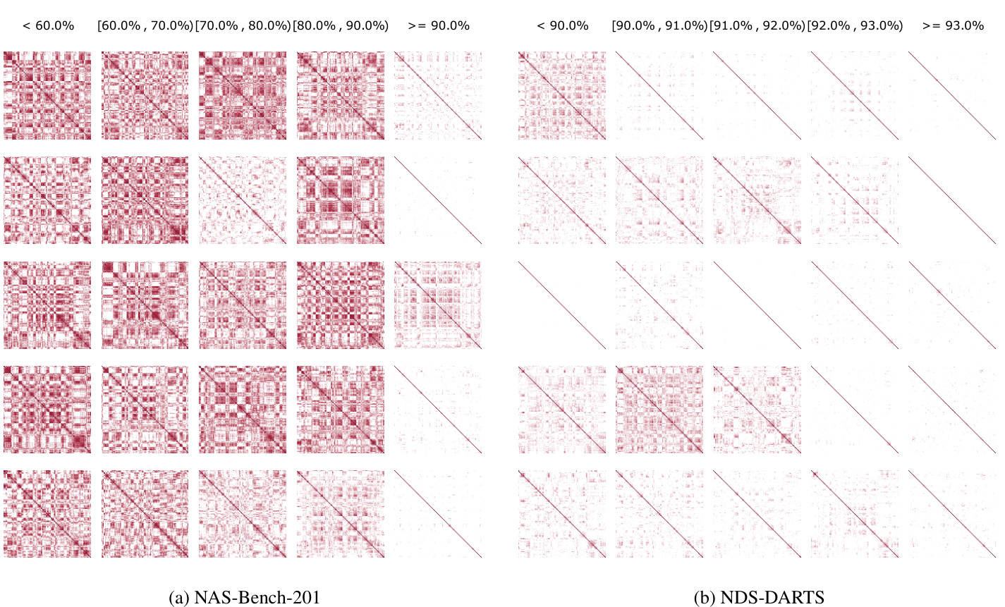
Figure 1. ${\bf K}_ {H}$ for a mini-batch of 128 CIFAR-10 images for untrained architectures in (a) NAS-Bench-201 (Dong & Yang, 2020) and (b) NDS-DARTS (Ra dosa vo vic et al., 2019). ${\bf K}_ {H}$ in these plots is normalised so that the diagonal entries are 1. The ${\bf K}_ {H}$ are sorted into columns based on the final CIFAR-10 validation accuracy when trained. Darker regions have higher similarity. The profiles are distinctive; the ${\bf K}_ {H}$ for good architectures in both search spaces have less similarity between different images. We can use ${\bf K}_ {H}$ for an untrained network to predict its final performance without any training. Note that (b) covers a tighter accuracy range than (a), which may explain it being less distinctive.
图 1: 在 (a) NAS-Bench-201 (Dong & Yang, 2020) 和 (b) NDS-DARTS (Ra dosa vo vic et al., 2019) 中,针对未训练架构的128张CIFAR-10图像小批量计算的 ${\bf K}_ {H}$。这些图中的 ${\bf K}_ {H}$ 经过归一化处理,使对角线元素为1。根据训练后的最终CIFAR-10验证准确率对 ${\bf K}_ {H}$ 进行列排序。颜色越深的区域表示相似度越高。不同架构的 ${\bf K}_ {H}$ 特征明显:两个搜索空间中优秀架构的 ${\bf K}_ {H}$ 在不同图像间表现出较低的相似性。我们可以利用未训练网络的 ${\bf K}_ {H}$ 来预测其最终性能,而无需任何训练。注意 (b) 图的准确率范围比 (a) 图更窄,这可能解释了其区分度较低的原因。
We believe that this work is an important proof-of-concept for NAS without training. The large resource and time costs associated with NAS can be avoided; our search algorithm uses a single GPU and is extremely fast. The benefit is twofold, as we also show that we can integrate our approach into existing NAS techniques for scenarios where obtaining as high an accuracy as possible is of the essence.
我们相信这项研究为无需训练的神经架构搜索(NAS)提供了重要概念验证。传统NAS伴随的巨大资源和时间成本得以规避——我们的搜索算法仅需单块GPU且速度极快。该方法具有双重优势:我们同时证明,在追求极致准确度的场景中,该技术可无缝集成至现有NAS框架。
2. Background
2. 背景
Designing a neural architecture by hand is a challenging and time-consuming task. It is extremely difficult to intuit where to place connections, or which operations to use. This has prompted an abundance of research into neural architecture search (NAS); the automation of the network design process. In the pioneering work of Zoph & Le (2017), the authors use an RNN controller to generate descriptions of candidate networks. Candidate networks are trained, and used to update the controller using reinforcement learning to improve the quality of the candidates it generates. This algorithm is very expensive: searching for an architecture to classify CIFAR-10 required running 800 GPUs for 28 days. It is also inflexible; the final network obtained is fixed and cannot be scaled e.g. for use on mobile devices or for other datasets.
手动设计神经网络架构是一项具有挑战性且耗时的任务。直觉上很难确定连接的位置或应使用的操作,这促使了大量关于神经架构搜索(NAS)的研究,即网络设计过程的自动化。在Zoph & Le (2017)的开创性工作中,作者使用RNN控制器生成候选网络的描述。候选网络经过训练后,通过强化学习更新控制器以提高其生成候选网络的质量。该算法成本极高:为CIFAR-10分类搜索架构需要800块GPU运行28天。此外,它缺乏灵活性;最终获得的网络是固定的,无法扩展,例如用于移动设备或其他数据集。
The subsequent work of Zoph et al. (2018) deals with these limitations. Inspired by the modular nature of successful hand-designed networks (Simonyan & Zisserman, 2015; He et al., 2016; Huang et al., 2017), they propose searching over neural building blocks, instead of over whole architectures. These building blocks, or cells, form part of a fixed overall network structure. Specifically, the authors search for a standard cell, and a reduced cell (incorporating pooling) for CIFAR-10 classification. These are then used as the building blocks of a larger network for ImageNet (Russ a kov sky et al., 2015) classification. While more flexible—the number of cells can be adjusted according to budget—and cheaper, owing to a smaller search space, this technique still utilised 500 GPUs across 4 days.
Zoph等人(2018)的后续工作解决了这些局限性。受成功手工设计网络的模块化特性启发(Simonyan & Zisserman, 2015; He等人, 2016; Huang等人, 2017), 他们提出搜索神经构建块而非完整架构。这些构建块(或称单元)构成固定整体网络结构的一部分。具体而言, 作者为CIFAR-10分类任务搜索标准单元和缩减单元(包含池化操作), 随后将这些单元作为更大网络的基本组件用于ImageNet(Russakovsky等人, 2015)分类任务。虽然这种方法更具灵活性(可根据预算调整单元数量)且因搜索空间更小而成本更低, 但仍需使用500块GPU运行4天。

Figure 2. Visual ising how binary activation codes of ReLU units correspond to linear regions. 1: Each ReLU node $\mathbf{A}i$ splits the input into an active $(>0)$ and inactive region We label the active region 1 and inactive 0. 2: The active/inactive regions associated with each node $\mathbf{A}i$ intersect. Areas of the input space with the same activation pattern are co-linear. Here we show the intersection of the A nodes and give the code for the linear regions. Bit $i$ of the code corresponds to whether node $\mathbf{A}i$ is active. 3: The ReLU nodes B of the next layer divides the space further into active and inactive regions. 4: Each linear region at a given node can be uniquely defined by the activation pattern of all the ReLU nodes that preceded it.
图 2: 可视化ReLU单元的二进制激活码如何对应线性区域。1: 每个ReLU节点$\mathbf{A}i$将输入划分为激活$(>0)$和非激活区域,我们用1标记激活区域,0标记非激活区域。2: 每个节点$\mathbf{A}i$相关的激活/非激活区域相交。具有相同激活模式的输入空间区域是共线的。这里我们展示了A节点的交集,并给出了线性区域的代码。代码的第$i$位对应于节点$\mathbf{A}i$是否激活。3: 下一层的ReLU节点B将空间进一步划分为激活和非激活区域。4: 给定节点的每个线性区域可以通过其之前所有ReLU节点的激活模式唯一定义。
ENAS (Pham et al., 2018) reduces the computational cost of searching by allowing multiple candidate architectures to share weights. This facilitates the simultaneous training of candidates, reducing the search time on CIFAR-10 to half a day on a single GPU. Weight sharing has seen widespread adoption in a host of NAS algorithms (Liu et al., 2019; Luo et al., 2018; Cai et al., 2019; Xie et al., 2019; Brock et al., 2018). However, there is evidence that it inhibits the search for optimal architectures (Yu et al., 2020), exposing random search as an extremely effective NAS baseline (Yu et al., 2020; Li & Talwalkar, 2019). There also remains the problem that the search spaces are still so vast—there are $1.6\times10^{29}$ possible architectures in Pham et al. (2018) for example—that it is impossible to identify the best networks and demonstrate that NAS algorithms find them.
ENAS (Pham等人,2018) 通过允许多个候选架构共享权重来降低搜索的计算成本。这使得候选架构能够同时训练,将CIFAR-10上的搜索时间缩短至单GPU半天。权重共享已在众多NAS算法中得到广泛应用 (Liu等人,2019; Luo等人,2018; Cai等人,2019; Xie等人,2019; Brock等人,2018)。然而,有证据表明它会抑制对最优架构的搜索 (Yu等人,2020),这暴露了随机搜索作为一种极其有效的NAS基线 (Yu等人,2020; Li & Talwalkar,2019)。此外,搜索空间仍然非常庞大——例如Pham等人 (2018) 中存在$1.6\times10^{29}$种可能的架构——以至于无法确定最佳网络并证明NAS算法能找到它们。
An orthogonal direction for identifying good architectures is the estimation of accuracy prior to training (Deng et al., 2017; Istrate et al., 2019), although these differ from this work in that they rely on training a predictive model, rather than investigating more fundamental architectural properties. Since its inception others have explored our work and the ideas therein in interesting directions. Of most interest from our perspective are Abdel fat tah et al. (2021) who integrate training-free heuristics into existing more-expensive search strategies to improve their performance as we do in this paper. Park et al. (2020) use the correspondence between wide neural networks and Gaussian processes to motivate using as a heuristic the validation accuracy of a Monte-Carlo approximated neural network Gaussian process conditioned on training data. Chen et al. (2021) propose two further heuristics—one based on the condition number of the neural tangent kernel (Jacot et al., 2018) at initial is ation and the other based on the number of unique linear regions that partition training data at initial is ation—with a proposed strategy to combine these heuristics into a stronger one.
识别优秀架构的另一个方向是在训练前预估准确率 (Deng et al., 2017; Istrate et al., 2019) ,但这些研究与本文的不同之处在于它们依赖于训练预测模型,而非探究更基础的架构特性。自本文发表以来,其他研究者从多个有趣的方向探索了我们的工作及其核心思想。在我们看来最具启发性的是Abdel fat tah等人 (2021) 的研究,他们将免训练启发式方法整合到现有高成本搜索策略中以提升性能,这与本文采用的方法一致。Park等人 (2020) 利用宽神经网络与高斯过程之间的对应关系,提出将蒙特卡洛近似神经网络高斯过程在训练数据条件下的验证准确率作为启发式指标。Chen等人 (2021) 提出了两个新启发式方法——一个基于神经网络正切核 (Jacot et al., 2018) 初始化时的条件数,另一个基于初始化时划分训练数据的唯一线性区域数量——并提出了将这些启发式方法组合成更强策略的方案。
2.1. NAS Benchmarks
2.1. NAS基准测试
A major barrier to evaluating the effectiveness of a NAS algorithm is that the search space (the set of all possible networks) is too large for exhaustive evaluation. This has led to the creation of several benchmarks (Ying et al., 2019; Zela et al., 2020; Dong & Yang, 2020; Dong et al., 2021) that consist of tractable NAS search spaces, and metadata for the training of networks within that search space. Concretely, this means that it is now possible to determine whether an algorithm is able to search for a good network. In this work we utilise NAS-Bench-101 (Ying et al., 2019), NASBench-201 (Dong & Yang, 2020), and NATS-Bench (Dong et al., 2021) to evaluate the effectiveness of our approach. NAS-Bench-101 consists of 423,624 neural networks that have been trained exhaustively, with three different initialisations, on the CIFAR-10 dataset for 108 epochs. NAS-Bench
评估NAS (Neural Architecture Search) 算法有效性的主要障碍在于搜索空间(所有可能网络的集合)过于庞大,无法进行穷举评估。这促使了多个基准数据集(Ying et al., 2019; Zela et al., 2020; Dong & Yang, 2020; Dong et al., 2021)的创建,这些数据集包含可处理的NAS搜索空间以及该搜索空间内网络训练的元数据。具体而言,这意味着现在可以确定某个算法是否能够搜索到优质网络。在本研究中,我们采用NAS-Bench-101 (Ying et al., 2019)、NAS-Bench-201 (Dong & Yang, 2020)和NATS-Bench (Dong et al., 2021)来评估我们方法的有效性。NAS-Bench-101包含423,624个神经网络,这些网络在CIFAR-10数据集上经过108个周期的训练(采用三种不同的初始化方式)并进行了穷举评估。
201 consists of 15,625 networks trained multiple times on CIFAR-10, CIFAR-100, and ImageNet-16-120 (Chrabaszcz et al., 2017). NATS-Bench (Dong et al., 2021) comprises two search spaces: a topology search space (NATS-Bench TSS) which contains the same 15,625 networks as NASBench 201; and a size search space (NATS-Bench SSS) which contains 32,768 networks where the number of channels for cells varies between these networks. These benchmarks are described in detail in Appendix A.
201包含15,625个在CIFAR-10、CIFAR-100和ImageNet-16-120 (Chrabaszcz et al., 2017) 上多次训练的网络。NATS-Bench (Dong et al., 2021) 包含两个搜索空间:拓扑搜索空间 (NATS-Bench TSS) 包含与NASBench 201相同的15,625个网络;以及规模搜索空间 (NATS-Bench SSS) 包含32,768个网络,这些网络中单元的通道数各不相同。这些基准测试的详细描述见附录A。
We also make use of the Network Design Spaces (NDS) dataset (Ra dosa vo vic et al., 2019). Where the NAS bench- marks aim to compare search algorithms, NDS aims to compare the search spaces themselves. All networks in NDS use the DARTS (Liu et al., 2019) skeleton. The networks are comprised of cells sampled from one of several NAS search spaces. Cells are sampled—and the resulting networks are trained—from each of AmoebaNet (Real et al., 2019); DARTS (Liu et al., 2019); ENAS (Pham et al., 2018), NASNet (Zoph & Le, 2017), and PNAS (Liu et al., 2018).
我们还利用了网络设计空间 (Network Design Spaces, NDS) 数据集 (Radosavovic et al., 2019)。NAS基准旨在比较搜索算法,而NDS则专注于比较搜索空间本身。NDS中的所有网络均采用DARTS (Liu et al., 2019) 骨架结构。这些网络由从多个NAS搜索空间中采样的单元组成,分别从AmoebaNet (Real et al., 2019)、DARTS (Liu et al., 2019)、ENAS (Pham et al., 2018)、NASNet (Zoph & Le, 2017) 和PNAS (Liu et al., 2018) 的搜索空间中采样单元并训练生成网络。
We denote each of these sets as NDS-AmoebaNet, NDSDARTS, NDS-ENAS, NDS-NASNet, and NDS-PNAS respectively. Note that these sets contain networks of variable width and depth, whereas in e.g. the original DARTS search space these were fixed quantities.1
我们将这些集合分别称为NDS-AmoebaNet、NDS-DARTS、NDS-ENAS、NDS-NASNet和NDS-PNAS。需要注意的是,这些集合包含不同宽度和深度的网络,而在原始DARTS搜索空间等情况下,这些是固定量。[1]
3. Scoring Networks at Initial is ation
3. 网络初始化评分
Our goal is to devise a means to score a network architecture at initial is ation in a way that is indicative of its final trained accuracy. This can either replace the expensive inner-loop training step in NAS, or better direct exploration in existing NAS algorithms.
我们的目标是设计一种方法,在网络架构初始化时对其进行评分,以预测其最终训练精度。这既可以替代神经架构搜索 (NAS) 中昂贵的内循环训练步骤,也能更好地指导现有NAS算法的探索方向。
Given a neural network with rectified linear units, we can, at each unit in each layer, identify a binary indicator as to whether the unit is inactive (the value is negative and hence is multiplied by zero) or active (in which case its value is multiplied by one). Fixing these indicator variables, it is well known that the network is now locally defined by a linear operator (Hanin & Rolnick, 2019); this operator is obtained by multiplying the linear maps at each layer interspersed with the binary rectification units. Consider a mini-batch of data $\mathbf{X}={\mathbf{x}_ {i}}_ {i=1}^{N}$ mapped through a neural network as $f(\mathbf{x}_ {i})$ . The indicator variables from the rectified linear units in $f$ at $\mathbf{x}_ {i}$ form a binary code $\mathbf{c}_ {i}$ that defines the linear region.
给定一个带有修正线性单元 (ReLU) 的神经网络,我们可以在每一层的每个单元上标识一个二元指示器,用于判断该单元是否处于非活跃状态(值为负因此乘以零)或活跃状态(此时其值乘以一)。固定这些指示变量后,众所周知,该网络现在由线性算子局部定义 (Hanin & Rolnick, 2019);该算子是通过将每层的线性映射与二元修正单元交错相乘得到的。考虑一个数据小批量 $\mathbf{X}={\mathbf{x}_ {i}}_ {i=1}^{N}$ 通过神经网络映射为 $f(\mathbf{x}_ {i})$。$f$ 中在 $\mathbf{x}_ {i}$ 处的修正线性单元的指示变量形成一个二进制代码 $\mathbf{c}_ {i}$,用于定义线性区域。
The intuition to our approach is that the more similar the binary codes associated with two inputs are then the more challenging it is for the network to learn to separate these inputs. When two inputs have the same binary code, they lie within the same linear region of the network and so are particularly difficult to disentangle. Conversely, learning should prove easier when inputs are well separated. Figure 2 visualises binary codes corresponding to linear regions.
我们方法的直观理解是,两个输入关联的二进制码越相似,网络就越难学会区分这些输入。当两个输入具有相同的二进制码时,它们位于网络的同一线性区域内,因此特别难以分离。相反,当输入被良好区分时,学习过程会更容易。图 2 展示了对应线性区域的二进制码可视化。
We use the Hamming distance $d_ {H}(\mathbf{c}_ {i},\mathbf{c}_ {j})$ between two binary codes—induced by the untrained network at two inputs—as a measure of how dissimilar the two inputs are.
我们使用两个二进制码之间的汉明距离 $d_ {H}(\mathbf{c}_ {i},\mathbf{c}_ {j})$ 来衡量两个输入之间的差异程度,该距离由未经训练的网络在两个输入处生成。
We can examine the correspondence between binary codes for the whole mini-batch by computing the kernel matrix
我们可以通过计算核矩阵来检查整个小批量二进制码之间的对应关系
$$
\mathbf{K}_ {H}=\left(\begin{array}{c c c}{N_ {A}-d_ {H}(\mathbf{c}_ {1},\mathbf{c}_ {1})}&{\cdots}&{N_ {A}-d_ {H}(\mathbf{c}_ {1},\mathbf{c}_ {N})}\ {\vdots}&{\ddots}&{\vdots}\ {N_ {A}-d_ {H}(\mathbf{c}_ {N},\mathbf{c}_ {1})}&{\cdots}&{N_ {A}-d_ {H}(\mathbf{c}_ {N},\mathbf{c}_ {N})}\end{array}\right)
$$
$$
\mathbf{K}_ {H}=\left(\begin{array}{c c c}{N_ {A}-d_ {H}(\mathbf{c}_ {1},\mathbf{c}_ {1})}&{\cdots}&{N_ {A}-d_ {H}(\mathbf{c}_ {1},\mathbf{c}_ {N})}\ {\vdots}&{\ddots}&{\vdots}\ {N_ {A}-d_ {H}(\mathbf{c}_ {N},\mathbf{c}_ {1})}&{\cdots}&{N_ {A}-d_ {H}(\mathbf{c}_ {N},\mathbf{c}_ {N})}\end{array}\right)
$$
where $N_ {A}$ is the number of rectified linear units.
其中 $N_ {A}$ 是修正线性单元的数量。
We compute ${\bf K}_ {H}$ for a random subset of NAS-Bench201 (Dong & Yang, 2020) and NDS-DARTS (Ra dosa vo vic et al., 2019) networks at initial is ation for a mini-batch of CIFAR-10 images. We plot normalised ${\bf K}_ {H}$ for different trained accuracy bounds in Figure 1.
我们计算了NAS-Bench201 (Dong & Yang, 2020) 和NDS-DARTS (Radosavovic et al., 2019) 网络在初始化时对一小批CIFAR-10图像的随机子集的 ${\bf K}_ {H}$ 。图1展示了不同训练精度界限下的归一化 ${\bf K}_ {H}$ 。
These normalised kernel plots are very distinct; high performing networks have fewer off-diagonal elements with high similarity. We can use this observation to predict the final performance of untrained networks, in place of the expensive training step in NAS. Specifically, we score networks using:
这些归一化核图差异显著:性能优异的网络具有更少的高相似度非对角元素。我们可以利用这一观察来预测未训练网络的最终性能,从而替代神经架构搜索(NAS)中昂贵的训练步骤。具体而言,我们通过以下公式对网络进行评分:
$$
s=\log|\mathbf{K}_ {H}|
$$
$$
s=\log|\mathbf{K}_ {H}|
$$
Given two kernels with the same trace, $s$ is higher for the kernel closest to diagonal. A higher score at initial is ation implies improved final accuracy after training.
给定两个具有相同迹的核,最接近对角线的核具有更高的$s$值。初始化时更高的分数意味着训练后最终准确率的提升。
For the search spaces across NAS-Bench-101 (Ying et al., 2019), NAS-Bench-201 (Dong & Yang, 2020), NATSBench SSS (Dong et al., 2021), and NDS (Ra dosa vo vic et al., 2019) we sample networks at random and plot our score $s$ on the untrained networks against their validation accuracies when trained. The plots for NAS-Bench-101, NAS-Bench-201, and NDS are available in Figure 3. In most cases 1000 networks are sampled.2 The plots for NATS-Bench SSS can be found in Figure 9 (Appendix B). We also provide comparison plots for the fixed width and depth spaces in NDS in Figure 10 (Appendix B). Kendall’s Tau correlation coefficients $\tau$ are given at the top of each plot.
在NAS-Bench-101 (Ying et al., 2019)、NAS-Bench-201 (Dong & Yang, 2020)、NATSBench SSS (Dong et al., 2021) 和NDS (Radosavovic et al., 2019) 的搜索空间中,我们随机采样网络,并将未训练网络的得分$s$与其训练后的验证准确率进行对比绘制。NAS-Bench-101、NAS-Bench-201和NDS的对比图见图3,大多数情况下采样了1000个网络。NATS-Bench SSS的对比图见图9(附录B)。此外,我们在图10(附录B)中提供了NDS固定宽度和深度空间的对比图。每个图的顶部给出了Kendall Tau相关系数$\tau$。
We find in all cases there is a positive correlation between the validation accuracy and the score. This is particularly strong for NAS-Bench-201 and NDS-DARTS. We show the Kendall’s Tau correlation coefficient between $s$ and final accuracy on CIFAR-10 for NDS in Figure 4. For comparison, we include the best-performing architecture scoring functions from Abdel fat tah et al. (2021) — grad norm and synflow — as baselines. The first is the sum of the gradient norms for every weight in the network, and the second is the summed Synaptic Flow score derived in Tanaka et al. (2020). our score (Equation 2) correlates with accuracy across all of the search spaces, where the other two scores fluctuate substantially. These results point to our score being effective on a wide array of neural network design spaces.
我们发现,在所有情况下,验证准确率与评分之间均存在正相关性。这种相关性在NAS-Bench-201和NDS-DARTS上尤为显著。图4展示了NDS中评分$s$与CIFAR-10最终准确率的Kendall's Tau相关系数。作为对比基线,我们引入了Abdel fat tah等人(2021)提出的最佳架构评分函数——梯度范数(grad norm)和突触流(synflow)。前者是网络中所有权重梯度范数的总和,后者源自Tanaka等人(2020)提出的突触流分数总和。我们的评分(公式2)在所有搜索空间中均与准确率保持稳定关联,而其他两种评分则波动较大。这些结果表明我们的评分在各类神经网络设计空间中都具备有效性。
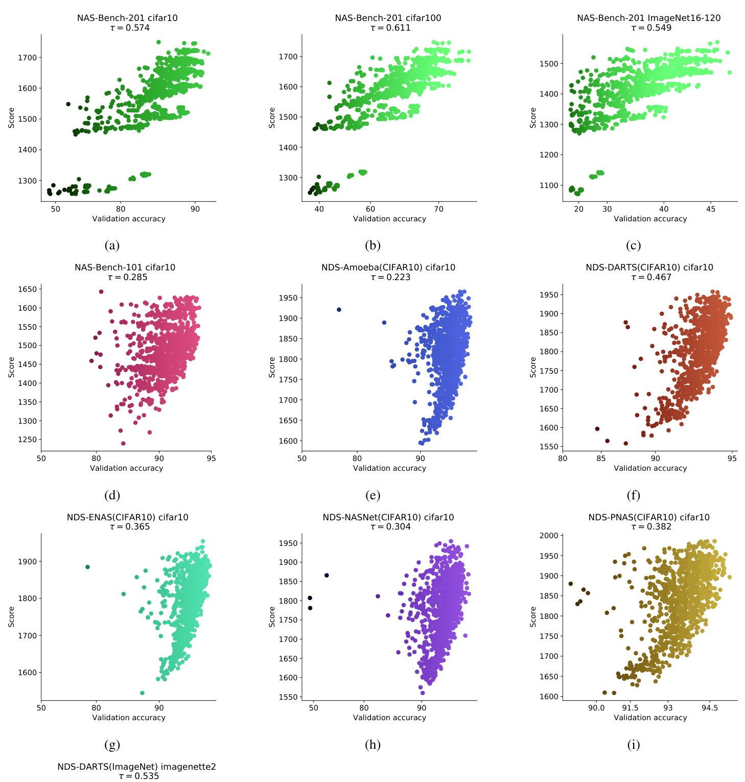
Figure 3. (a)-(i): Plots of our score for randomly sampled untrained architectures in NAS-Bench-201, NAS-Bench-101, NDS-Amoeba, NDS-DARTS, NDS-ENAS, NDS-NASNet, NDS-PNAS against validation accuracy when trained. The inputs when computing the score and the validation accuracy for each plot are from CIFAR-10 except for (b) and (c) which use CIFAR-100 and ImageNet16-120 respectively. (j): We include a plot from NDS-DARTS on ImageNet (121 networks provided) to illustrate that the score extends to more challenging datasets. We use a mini-batch from Image Net te 2 which is a strict subset of ImageNet with only 10 classes. In all cases there is a noticeable correlation between the score for an untrained network and the final accuracy when trained.
图 3: (a)-(i) 展示了我们在NAS-Bench-201、NAS-Bench-101、NDS-Amoeba、NDS-DARTS、NDS-ENAS、NDS-NASNet、NDS-PNAS中对随机采样的未训练架构的评分与训练后验证准确率的对比图。除(b)和(c)分别使用CIFAR-100和ImageNet16-120外,其他各图的评分计算输入和验证准确率均来自CIFAR-10。(j) 我们加入了NDS-DARTS在ImageNet上的结果图(包含121个网络),以说明该评分方法可扩展至更具挑战性的数据集。我们使用了ImageNet te 2的一个小批量数据,这是仅包含10个类别的ImageNet严格子集。所有情况下,未训练网络的评分与最终训练准确率均存在显著相关性。

Figure 4. Kendall’s Tau correlation across each of the NDS CIFAR-10 search spaces. We compare our method to two alternative measures: grad norm and synflow. The results for grad norm refer to the absolute Euclidean-norm of the gradients over one random mini-batch of data. synflow is the gradient-based score defined by Tanaka et al. (2020), summed over each parameter in the network.
图 4: NDS CIFAR-10各搜索空间中的Kendall's Tau相关性。我们将本方法与两种替代指标进行对比:梯度范数(grad norm)和SynFlow。梯度范数结果表示随机小批量数据梯度的绝对欧几里得范数。SynFlow是Tanaka等人(2020)提出的基于梯度的评分指标,通过对网络中每个参数求和计算得出。
3.1. Ablation Study
3.1. 消融研究
How important are the images used to compute the score? Since our approach relies on randomly sampling a single mini-batch of data, it is reasonable to question whether different mini-batches result in different scores. To determine whether our method is dependent on minibatches, we randomly select 10 architectures from different CIFAR-100 accuracy percentiles in NAS-Bench-201 and compute the score separately for 20 random CIFAR-100 mini-batches. The resulting box-and-whisker plot is given in Figure 5(top-left): the ranking of the scores is reasonably robust to the specific choice of images. In Figure 5(topright) we compute our score using normally distributed random inputs; this has little impact on the general trend. This suggests our score captures a property of the network architecture, rather than something data-specific.
用于计算分数的图像有多重要?由于我们的方法依赖于随机采样单个小批量数据,因此合理质疑不同的小批量是否会导致不同的分数。为了确定我们的方法是否依赖于小批量,我们从NAS-Bench-201中随机选取10个来自不同CIFAR-100准确率百分位的架构,并分别对20个随机CIFAR-100小批量计算分数。结果箱线图如图5(左上)所示:分数排序对图像的具体选择具有较好的鲁棒性。在图5(右上)中,我们使用正态分布的随机输入计算分数;这对总体趋势几乎没有影响。这表明我们的分数捕捉的是网络架构的特性,而非数据特定的属性。
Does the score change for different initial is at ions? Figure 5(bottom-left) shows how the score for our 10 NASBench-201 architectures differs over 20 initial is at ions. While there is some noise, the better performing networks remain distinctive, and can be isolated.
不同初始条件下得分会变化吗?图5(左下)展示了我们10种NASBench-201架构在20种初始条件下的得分差异。虽然存在一些噪声,但性能更好的网络仍然具有区分度,并且可以被分离出来。
Does the size of the mini-batch matter? As ${\bf K}_ {H}$ scales with mini-batch size we compare across mini-batch sizes by dividing a given score by the minimum score using the same mini-batch size from the set of sampled networks. Figure 5(bottom-right) presents this normalised score for different mini-batch sizes. The best performing networks remain distinct.
小批量(mini-batch)的规模重要吗?由于 ${\bf K}_ {H}$ 会随小批量规模变化,我们通过将给定分数除以使用相同小批量规模的采样网络集合中的最低分数来进行跨规模比较。图5(右下)展示了不同小批量规模下的归一化分数表现,最优网络依然保持显著区分。
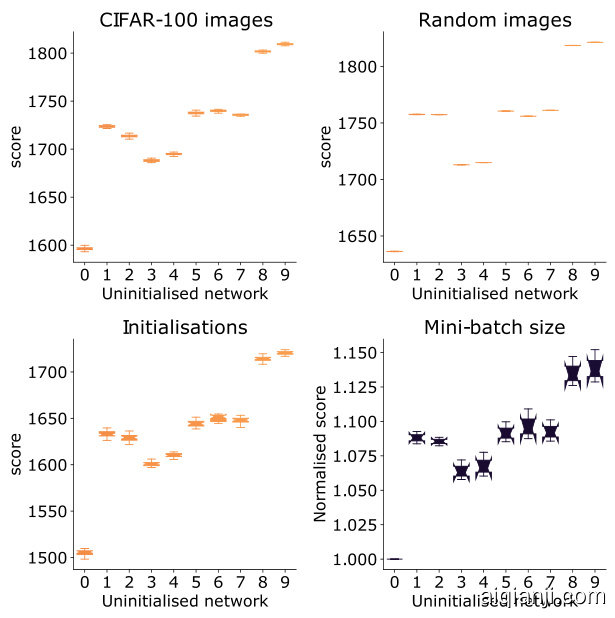
Figure 5. Ablation experiments showing the effect on our score using different CIFAR-100 mini-batches (top-left), random normallydistributed input images (top-right), weight initial is at ions (bottomleft), and mini-batch sizes (bottom-right) for 10 randomly selected NAS-Bench-201 architectures (one in each $5%$ percentile range from 50-55, ..., 95-100). For each network, 20 samples were taken for each ablation. The mini-batch size was 128 for all experiments apart from the bottom-right. The bottom-right experiment used mini-batch sizes of 32, 64, 128, and 256; as the score depends on the mini-batch size we normalised the score by the minimum score of the sampled networks from the same mini-batch size.
图 5: 消融实验展示了不同CIFAR-100小批次(左上)、随机正态分布输入图像(右上)、权重初始化(左下)和小批次尺寸(右下)对10个随机选择的NAS-Bench-201架构(每个$5%$百分位区间选取一个,范围从50-55,...,95-100)评分的影响。每个网络针对每种消融情况采样20次。除右下实验外,其余实验均使用128的小批次尺寸。右下实验使用32/64/128/256四种小批次尺寸;由于评分与小批次尺寸相关,我们通过同尺寸采样网络的最小评分对结果进行了归一化处理。
How does the score evolve as networks are trained? Although the motivation of our work is to score un initial is ed networks, it is worth observing how the score evolves as a network is trained. We consider 10 NAS-Bench-201 networks with $>90%$ validation accuracy when evaluated on CIFAR-10. This makes the performance difference between the 10 networks much smaller than for the search space as a whole. We train each network via stochastic gradient descent with a cross entropy loss for 100 epochs and evaluate the score at each training epoch. Figure 6 shows the evolution of the score. The left subplot shows a zoomed-in view of the score trajectories across the first two epochs and the right subplot shows the score trajectories across all 100 epochs. We observe that the score increases in all cases immediately after some training has occurred, but very quickly stabilises to a near constant value. The increase in the score value after initial is ation was similar amongst the networks, and the relative ranking remained similar throughout.
网络训练过程中评分如何变化?尽管我们工作的初衷是评估未经初始化的网络,但观察网络训练过程中评分的变化也很有价值。我们选取了10个在CIFAR-10数据集上验证准确率超过90%的NAS-Bench-201网络进行研究。这使得10个网络间的性能差异远小于整个搜索空间的差异。我们采用随机梯度下降法和交叉熵损失函数对每个网络进行100轮训练,并在每轮训练后评估其得分。图6展示了评分的变化趋势:左子图聚焦前两轮的评分轨迹,右子图则呈现全部100轮的评分轨迹。研究发现,所有网络在经过初步训练后评分均会立即上升,但很快会稳定在接近恒定的数值。各网络在初始化后的评分增幅相似,且相对排名在整个训练过程中保持稳定。

Figure 6. Plots of our score (Equation 2) during training for 10 networks from NAS-Bench-201 using the CIFAR-10 dataset. The legend provides the final accuracy of the network as given by the NAS-Bench-201 API. For all 10 networks the score increases sharply in the first few epochs and then flattens. The ranking of the scores between networks remains relatively stable throughout training.
图 6: 使用CIFAR-10数据集训练的10个NAS-Bench-201网络得分(公式2)曲线图。图例显示NAS-Bench-201 API提供的网络最终准确率。所有10个网络的得分在前几个训练周期急剧上升后趋于平缓。网络间的得分排名在整个训练过程中保持相对稳定。
In Section 4 we demonstrate how our score (Equation 2) can be used in a NAS algorithm for extremely fast search.
在第4节中,我们展示了如何将我们的评分(公式2)应用于NAS算法以实现极速搜索。
4. Neural Architecture Search without Training — NASWOT
4. 无需训练的神经架构搜索 — NASWOT
In Section 3 we derived a score for cheaply ranking networks at initial is ation based on their expected performance (Equation 2). Here as a proof of concept, we integrate this score into a simple search algorithm and evaluate its ability to alleviate the need for training in NAS. Code for reproducing our experiments is available at https://github. com/BayesWatch/nas-without-training.
在第3节中,我们推导出一个评分(公式2),用于在初始化阶段低成本地对网络进行预期性能排序。作为概念验证,我们将该评分集成到一个简单搜索算法中,并评估其在神经架构搜索(NAS)中减少训练需求的能力。实验复现代码详见 https://github.com/BayesWatch/nas-without-training。
Table 1. Mean $\pm$ std. accuracy from NAS-Bench-101. NASWOT is our training-free algorithm (across 500 runs). REA uses evolutionary search to select an architecture (50 runs), Random selects one architecture $(500\mathrm{runs})$ . AREA (assisted-REA) uses our score (Equation 2) to select the starting population for REA (50 runs). Search times for REA and AREA were calculated using the NASBench-101 API.
| Method | Search (s) | CIFAR-10 |
| Random | N/A | 90.38±5.51 |
| NASWOT (N=100) | 23 | 91.77±0.05 |
| REA | 12000 | 93.87±0.22 |
| AREA (Ours) | 12000 | 93.91±0.29 |
表 1: NAS-Bench-101 的平均准确率 $\pm$ 标准差。NASWOT 是我们的免训练算法 (基于 500 次运行)。REA 使用进化搜索选择架构 (50 次运行),Random 随机选择一个架构 $(500\mathrm{次运行})$。AREA (辅助-REA) 使用我们的评分 (公式 2) 为 REA 选择初始种群 (50 次运行)。REA 和 AREA 的搜索时间通过 NASBench-101 API 计算。
| 方法 | 搜索时间 (秒) | CIFAR-10 |
|---|---|---|
| Random | N/A | 90.38±5.51 |
| NASWOT (N=100) | 23 | 91.77±0.05 |
| REA | 12000 | 93.87±0.22 |
| AREA (Ours) | 12000 | 93.91±0.29 |
| lgorithm1NASWOT |
| generator = RandomGeneratorO |
| best_ net,best_ score =None,0 |
| fori=1:Ndo |
| net = generator.generate() |
| score=net.score() |
| ifscore>best-scorethen |
| best_ net,best_ score=net,score chosen_ net=best_ network |
| lgorithm1NASWOT |
|---|
| generator = RandomGeneratorO |
| best_ net, best_ score = None, 0 |
| for i = 1:N do |
| net = generator.generate() |
| score = net.score() |
| if score > best_ score then |
| best_ net, best_ score = net, score chosen_ net = best_ network |
Many NAS algorithms are based on that of Zoph & Le (2017); it uses a generator network which proposes architectures. The weights of the generator are learnt by training the networks it generates, either on a proxy task or on the dataset itself, and using their trained accuracies as signal through e.g. REINFORCE (Williams, 1992). This is repeated until the generator is trained; it then produces a final network which is the output of this algorithm. The vast majority of the cost is incurred by having to train candidate architectures for every single controller update. Note that there exist alternative schema utilising e.g. evolutionary algorithms (Real et al., 2019) or bilevel optimisation (Liu et al., 2019) but all involve training.
许多神经架构搜索(NAS)算法都基于Zoph & Le (2017)的研究,该研究使用生成网络来提出架构方案。生成器的权重通过训练其生成的网络来学习,训练过程要么在代理任务上进行,要么直接在目标数据集上进行,并使用这些网络的训练准确率作为信号(例如通过REINFORCE算法 (Williams, 1992))。这一过程不断重复,直到生成器完成训练;随后生成器会输出一个最终网络作为算法结果。该方法的绝大部分计算成本都来自于每次控制器更新时需要对候选架构进行训练。需要注意的是,还存在其他替代方案,例如使用进化算法 (Real et al., 2019) 或双层优化 (Liu et al., 2019),但这些方法同样需要进行训练。
We instead propose a simple alternative—NASWOT— illustrated in Algorithm 1. Instead of having a neural network as a generator, we randomly propose a candidate from the search space and then rather than training it, we score it in its untrained state using Equation 2. We do this N times—i.e. we have a sample size of N architectures—and then output the highest scoring network.
我们提出了一种简单的替代方案——NASWOT——如算法1所示。我们不使用神经网络作为生成器,而是从搜索空间中随机提出候选架构,然后不进行训练,而是用公式2对其在未训练状态下进行评分。我们重复此过程N次(即采样N个架构),然后输出得分最高的网络。
NAS-Bench-101. We compare NASWOT to 12000 seconds of REA (Real et al., 2019) and random selection on NAS-Bench-101 (Ying et al., 2019) in Table 1. NASWOT can find a network with a final accuracy roughly midway between these methods in under a minute on a single GPU.
NAS-Bench-101。我们在表1中将NASWOT与12000秒的REA (Real et al., 2019) 以及NAS-Bench-101 (Ying et al., 2019) 上的随机选择进行了对比。NASWOT在单GPU上只需不到一分钟即可找到最终准确率大致介于这些方法之间的网络。
NAS-Bench-201. Dong & Yang (2020) benchmark a wide range of NAS algorithms, both with and without weight sharing, that we compare to NASWOT. The weight sharing methods are random search with parameter sharing (RSPS, Li & Talwalkar, 2019), first-order DARTS (DARTSV1, Liu et al., 2019), second order DARTS (DARTS-V2, Liu et al., 2019), GDAS (Dong & Yang, 2019b), SETN (Dong & Yang, 2019a), and ENAS (Pham et al., 2018). The nonweight sharing methods are random search with training (RS), REA (Real et al., 2019), REINFORCE (Williams, 1992), and BOHB (Falkner et al., 2018). For implementation details we refer the reader to Dong & Yang (2020). The hyper parameters in NAS-Bench-201 are fixed — these results may not be invariant to hyper parameter choices, which may explain the low performance of e.g. DARTS.
NAS-Bench-201。Dong & Yang (2020) 对多种神经架构搜索 (NAS) 算法进行了基准测试 (包括权重共享和非权重共享方法),我们将这些方法与NASWOT进行比较。权重共享方法包括:带参数共享的随机搜索 (RSPS, Li & Talwalkar, 2019)、一阶DARTS (DARTSV1, Liu et al., 2019)、二阶DARTS (DARTS-V2, Liu et al., 2019)、GDAS (Dong & Yang, 2019b)、SETN (Dong & Yang, 2019a) 和 ENAS (Pham et al., 2018)。非权重共享方法包括:带训练的随机搜索 (RS)、REA (Real et al., 2019)、REINFORCE (Williams, 1992) 和 BOHB (Falkner et al., 2018)。具体实现细节请参阅 Dong & Yang (2020)。NAS-Bench-201中的超参数是固定的——这些结果可能对超参数选择不具有不变性,这或许解释了某些方法 (如DARTS) 表现不佳的原因。
Table 2. (a): Mean $\pm$ std. accuracies on NAS-Bench-201. Baselines are taken directly from Dong & Yang (2020), averaged over 500 runs (3 for weight-sharing methods). Search times are recorded for a single 1080Ti GPU. Note that all searches are performed on CIFAR-10 before evaluating the final model on CIFAR-10, CIFAR-100, and ImageNet-16-120. The performance of our training-free approach (NASWOT) is given for different sample size N (also 500 runs), along with that of our Assisted REA (AREA) approach (50 runs). We also report the results for picking a network at random, and the best possible network from the sample. (b): Mean $\pm$ std. accuracies (over 500 runs) on NATS-Bench SSS (Dong et al., 2021) comparing non-weight sharing approaches to NASWOT. Unlike NAS-Bench-201, each search is performed on the same dataset that is then used to evaluate the proposed network.
| Method | Search (s) | CIFAR-10 | CIFAR-100 | ImageNet-16-120 | |||
| validation | test | validation | test | validation | test | ||
| (a) NAS-Bench-201 | |||||||
| Non-weight sharing | |||||||
| REA | 12000 | 91.19±0.31 | 93.92±0.30 | 71.81±1.12 | 71.84±0.99 | 45.15±0.89 | 45.54±1.03 |
| RS | 12000 | 90.93±0.36 | 93.70±0.36 | 70.93±1.09 | 71.04±1.07 | 44.45±1.10 | 44.57±1.25 |
| REINFORCE | 12000 | 91.09±0.37 | 93.85±0.37 | 71.61±1.12 | 71.71±1.09 | 45.05±1.02 | 45.24±1.18 |
| BOHB | 12000 | 90.82±0.53 | 93.61±0.52 | 70.74±1.29 | 70.85±1.28 | 44.26±1.36 | 44.42±1.49 |
| Weight sharing | |||||||
| RSPS | 7587 | 84.16±1.69 | 87.66±1.69 | 59.00±4.60 | 58.33±4.34 | 31.56±3.28 | 31.14±3.88 |
| DARTS-V1 | 10890 | 39.77±0.00 | 54.30±0.00 | 15.03±0.00 | 15.61±0.00 | 16.43±0.00 | 16.32±0.00 |
| DARTS-V2 | 29902 | 39.77±0.00 | 54.30±0.00 | 15.03±0.00 | 15.61±0.00 | 16.43±0.00 | 16.32±0.00 |
| GDAS | 28926 | 90.00±0.21 | 93.51±0.13 | 71.14±0.27 | 70.61±0.26 | 41.70±1.26 | 41.84±0.90 |
| SETN | 31010 | 82.25±5.17 | 86.19±4.63 | 56.86±7.59 | 56.87±7.77 | 32.54±3.63 | 31.90±4.07 |
| ENAS | 13315 | 39.77±0.00 | 54.30±0.00 | 15.03±0.00 | 15.61±0.00 | 16.43±0.00 | 16.32±0.00 |
| Training-free | |||||||
| NASWOT (N=10) | 3.05 | 89.14 ± 1.14 | 92.44 ± 1.13 | 68.50 ± 2.03 | 68.62 ± 2.04 | 41.09 ± 3.97 | 41.31 ± 4.11 |
| NASWOT (N=100) | 30.01 | 89.55 ± 0.89 | 92.81 ± 0.99 | 69.35 ± 1.70 | 69.48 ± 1.70 | 42.81 ± 3.05 | 43.10 ± 3.16 |
| NASWOT (N=1000) | 306.19 | 89.69 ± 0.73 | 92.96 ± 0.81 | 69.86 ± 1.21 | 69.98 ± 1.22 | 43.95 ± 2.05 | 44.44 ± 2.10 |
| Random | N/A | 83.20 ± 13.28 | 86.61 ± 13.46 | 60.70 ± 12.55 | 60.83 ± 12.58 | 33.34 ± 9.39 | 33.13 ± 9.66 |
| Optimal (N=10) | N/A | 89.92 ± 0.75 | 93.06 ± 0.59 | 69.61 ± 1.21 | 69.76 ± 1.25 | 43.11 ± 1.85 | 43.30 ± 1.87 |
| Optimal (N=100) | N/A | 91.05 ± 0.28 | 93.84 ± 0.23 | 71.45 ± 0.79 | 71.56 ± 0.78 | 45.37 ± 0.61 | 45.67 ± 0.64 |
| AREA | 12000 | 91.20 ± 0.27 | 71.95 ± 0.99 | - | 45.70 ± 1.05 | - | |
| (b) NATS-Bench SSS | |||||||
| Non-weight sharing | |||||||
| REA | 12000 | 90.37±0.20 | 93.22±0.16 | 70.23±0.50 | 70.11±0.61 | 45.30±0.69 | 45.54±0.92 |
| RS | 12000 | 90.10±0.26 | 93.03±0.25 | 69.57±0.57 | 69.72±0.61 | 45.01±0.74 | 45.42±0.86 |
| REINFORCE | 12000 | 90.25±0.23 | 93.16±0.21 | 69.84±0.59 | 69.96±0.57 | 45.06±0.77 | 45.24±1.18 |
| BOHB | 12000 | 90.07±0.28 | 93.01±0.24 | 69.75±0.60 | 69.90±0.60 | 45.11±0.69 | 45.56±0.81 |
| NASWOT (N=10) | 3.02 | 88.95 ± 0.88 | 88.66 ± 0.90 | 64.55 ± 4.57 | 64.54 ± 4.70 | 40.22 ± 3.73 | 40.48 ± 3.73 |
| NASWOT (N=100) | 32.36 | 89.68 ± 0.51 | 89.38 ± 0.54 | 66.71 ± 3.05 | 66.68 ± 3.25 | 42.68 ± 2.58 | 43.11 ± 2.42 |
| NASWOT (N=1000) | 248.23 | 90.14 ± 0.30 | 93.10 ± 0.31 | 68.96 ± 1.54 | 69.10 ± 1.61 | 44.57 ± 1.48 | 45.08 ± 1.55 |
表 2. (a): NAS-Bench-201上的平均$\pm$标准差准确率。基线结果直接取自Dong & Yang (2020),基于500次运行取平均值(权重共享方法为3次)。搜索时间记录于单块1080Ti GPU。注意所有搜索均在CIFAR-10上执行,最终模型在CIFAR-10、CIFAR-100和ImageNet-16-120上评估。我们提出的免训练方法(NASWOT)在不同样本量N(同样500次运行)下的表现,以及辅助REA(AREA)方法(50次运行)的表现均有列出。同时报告了随机选择网络和样本中最优网络的结果。(b): NATS-Bench SSS上非权重共享方法与NASWOT的比较结果(基于500次运行的平均$\pm$标准差准确率)。与NAS-Bench-201不同,每次搜索在与评估网络相同的数据集上进行。
| 方法 | 搜索时间(s) | CIFAR-10验证集 | CIFAR-10测试集 | CIFAR-100验证集 | CIFAR-100测试集 | ImageNet-16-120验证集 | ImageNet-16-120测试集 |
|---|---|---|---|---|---|---|---|
| * * (a) NAS-Bench-201* * | |||||||
| * * 非权重共享* * | |||||||
| REA | 12000 | 91.19±0.31 | 93.92±0.30 | 71.81±1.12 | 71.84±0.99 | 45.15±0.89 | 45.54±1.03 |
| RS | 12000 | 90.93±0.36 | 93.70±0.36 | 70.93±1.09 | 71.04±1.07 | 44.45±1.10 | 44.57±1.25 |
| REINFORCE | 12000 | 91.09±0.37 | 93.85±0.37 | 71.61±1.12 | 71.71±1.09 | 45.05±1.02 | 45.24±1.18 |
| BOHB | 12000 | 90.82±0.53 | 93.61±0.52 | 70.74±1.29 | 70.85±1.28 | 44.26±1.36 | 44.42±1.49 |
| * * 权重共享* * | |||||||
| RSPS | 7587 | 84.16±1.69 | 87.66±1.69 | 59.00±4.60 | 58.33±4.34 | 31.56±3.28 | 31.14±3.88 |
| DARTS-V1 | 10890 | 39.77±0.00 | 54.30±0.00 | 15.03±0.00 | 15.61±0.00 | 16.43±0.00 | 16.32±0.00 |
| DARTS-V2 | 29902 | 39.77±0.00 | 54.30±0.00 | 15.03±0.00 | 15.61±0.00 | 16.43±0.00 | 16.32±0.00 |
| GDAS | 28926 | 90.00±0.21 | 93.51±0.13 | 71.14±0.27 | 70.61±0.26 | 41.70±1.26 | 41.84±0.90 |
| SETN | 31010 | 82.25±5.17 | 86.19±4.63 | 56.86±7.59 | 56.87±7.77 | 32.54±3.63 | 31.90±4.07 |
| ENAS | 13315 | 39.77±0.00 | 54.30±0.00 | 15.03±0.00 | 15.61±0.00 | 16.43±0.00 | 16.32±0.00 |
| * * 免训练* * | |||||||
| NASWOT (N=10) | 3.05 | 89.14±1.14 | 92.44±1.13 | 68.50±2.03 | 68.62±2.04 | 41.09±3.97 | 41.31±4.11 |
| NASWOT (N=100) | 30.01 | 89.55±0.89 | 92.81±0.99 | 69.35±1.70 | 69.48±1.70 | 42.81±3.05 | 43.10±3.16 |
| NASWOT (N=1000) | 306.19 | 89.69±0.73 | 92.96±0.81 | 69.86±1.21 | 69.98±1.22 | 43.95±2.05 | 44.44±2.10 |
| Random | N/A | 83.20±13.28 | 86.61±13.46 | 60.70±12.55 | 60.83±12.58 | 33.34±9.39 | 33.13±9.66 |
| Optimal (N=10) | N/A | 89.92±0.75 | 93.06±0.59 | 69.61±1.21 | 69.76±1.25 | 43.11±1.85 | 43.30±1.87 |
| Optimal (N=100) | N/A | 91.05±0.28 | 93.84±0.23 | 71.45±0.79 | 71.56±0.78 | 45.37±0.61 | 45.67±0.64 |
| AREA | 12000 | 91.20±0.27 | - | 71.95±0.99 | - | 45.70±1.05 | - |
| * * (b) NATS-Bench SSS* * | |||||||
| * * 非权重共享* * | |||||||
| REA | 12000 | 90.37±0.20 | 93.22±0.16 | 70.23±0.50 | 70.11±0.61 | 45.30±0.69 | 45.54±0.92 |
| RS | 12000 | 90.10±0.26 | 93.03±0.25 | 69.57±0.57 | 69.72±0.61 | 45.01±0.74 | 45.42±0.86 |
| REINFORCE | 12000 | 90.25±0.23 | 93.16±0.21 | 69.84±0.59 | 69.96±0.57 | 45.06±0.77 | 45.24±1.18 |
| BOHB | 12000 | 90.07±0.28 | 93.01±0.24 | 69.75±0.60 | 69.90±0.60 | 45.11±0.69 | 45.56±0.81 |
| NASWOT (N=10) | 3.02 | 88.95±0.88 | 88.66±0.90 | 64.55±4.57 | 64.54±4.70 | 40.22±3.73 | 40.48±3.73 |
| NASWOT (N=100) | 32.36 | 89.68±0.51 | 89.38±0.54 | 66.71±3.05 | 66.68±3.25 | 42.68±2.58 | 43.11±2.42 |
| NASWOT (N=1000) | 248.23 | 90.14±0.30 | 93.10±0.31 | 68.96±1.54 | 69.10±1.61 | 44.57±1.48 | 45.08±1.55 |
All searches are performed on CIFAR-10, and the output architecture is then trained and evaluated on each of CIFAR10, CIFAR-100, and ImageNet-16-120 for different dataset splits. We report results in Table 2(a). Search times are reported for a single GeForce GTX 1080 Ti GPU. As per the NAS-Bench-201 setup, the non-weight sharing methods are given a time budget of 12000 seconds. For NASWOT and the non-weight sharing methods, accuracies are averaged over 500 runs. For weight-sharing methods, accuracies are reported over 3 runs. We report NASWOT for sample sizes of $\mathrm{N}{=}10$ , $\scriptstyle\mathrm{N}=100$ , and $\scriptstyle\mathrm{N}=1000$ . NASWOT is able to outperform all of the weight sharing methods while requiring a fraction of the search time.
所有搜索均在CIFAR-10上执行,随后针对不同数据集划分,在CIFAR-10、CIFAR-100和ImageNet-16-120上训练并评估输出架构。结果如 表 2(a) 所示。搜索时间基于单块GeForce GTX 1080 Ti GPU测得。根据NAS-Bench-201设定,非权重共享方法的时间预算为12000秒。对于NASWOT和非权重共享方法,准确率为500次运行的平均值;权重共享方法则报告3次运行的准确率。我们展示了NASWOT在样本量$\mathrm{N}{=}10$、$\scriptstyle\mathrm{N}=100$和$\scriptstyle\mathrm{N}=1000$下的表现。NASWOT在仅需部分搜索时间的情况下,性能优于所有权重共享方法。
The non-weight sharing methods do outperform NASWOT, though they also incur a large search time cost. It is encouraging however, that in a matter of seconds, NASWOT is able to find networks with performance close to the best non-weight sharing algorithms, suggesting that network archi tec ture s themselves contain almost as much information about final performance at initial is ation as after training.
非权重共享方法确实优于NASWOT,但它们也带来了巨大的搜索时间成本。然而令人鼓舞的是,NASWOT仅需数秒就能找到性能接近最佳非权重共享算法的网络架构,这表明网络结构本身在初始化阶段就包含了几乎与训练后同等丰富的最终性能信息。
Table 2(a) also shows the effect of sample size (N). We show the accuracy of networks chosen by our method for each N. We list optimal accuracy for each N, and random selection over the whole benchmark, both averaged over 500 runs. We observe that sample size increases NASWOT performance.
表 2(a) 同时展示了样本量 (N) 的影响。我们列出了本方法针对每个 N 值所选网络的准确率,以及在整个基准测试中随机选择的各 N 值最优准确率 (均经过 500 次运行取平均) 。可以观察到样本量的增加能提升 NASWOT 的表现。
NATS-Bench. Dong et al. (2021) expanded on the original NAS-Bench-201 work to include a further search space: NATS-Bench SSS. The same non-weight sharing methods were evaluated as in NAS-Bench-201. Unlike NASBench-201, search and evaluation are performed on the same dataset. Implementation details are available in Dong et al. (2021). We observe that sample size increases NASWOT performance significantly on NATS-Bench SSS, to the point where it is extremely similar to other methods.
NATS-Bench。Dong等人(2021)在原始NAS-Bench-201工作基础上扩展了另一个搜索空间:NATS-Bench SSS。与NAS-Bench-201相同,评估了非权重共享方法。不同于NASBench-201,其搜索和评估在同一数据集上进行。具体实现细节见Dong等人(2021)的论文。我们观察到,在NATS-Bench SSS上,样本量显著提升了NASWOT的性能,使其与其他方法极为接近。
A key practical benefit of NASWOT is its rapid execution time. This may be important when repeating NAS several times, for instance for several hardware devices or datasets. This affords us the ability in future to specialise neural architectures for a task and resource environment cheaply, demanding only a few seconds per setup. Figure 7 shows our method in contrast to other NAS methods for NASBench-201, showing the trade-off between final network accuracy and search time.
NASWOT的一个关键实际优势是其快速的执行时间。这在需要多次重复NAS时可能很重要,例如针对多个硬件设备或数据集。这使得我们未来能够以低廉的成本为特定任务和资源环境定制神经网络架构,每个设置仅需几秒钟。图7展示了我们的方法与其他NAS方法在NASBench-201上的对比,显示了最终网络准确性与搜索时间之间的权衡。
4.1. Assisted Regular is ed EA — AREA
4.1. 辅助正则化EA (Assisted Regular is ed EA) — AREA
Our proposed score can be straightforwardly incorporated into existing NAS algorithms. To demonstrate this we implemented a variant of REA (Real et al., 2019), which we call Assisted-REA (AREA). REA starts with a randomlyselected population (10 in our experiments). AREA instead randomly-samples a larger population (in our experiments we double the randomly-selected population size to 20) and uses our score (Equation 2) to select the initial population (of size 10) for the REA algorithm. Pseudocode can be found in Algorithm 2 with results on NAS-Bench-101 and NAS-Bench-201 in Tables 1 and 2. AREA outerforms REA on NAS-Bench-201 (CIFAR-100, ImageNet-16-120) but is very similar to REA on NAS-Bench-101. We hope that future work will build on this algorithm further.
我们提出的评分可以轻松整合到现有的NAS算法中。为验证这一点,我们实现了REA (Real等人,2019) 的变体,称为辅助REA (AREA)。REA从随机选择的初始种群开始 (实验中设为10个),而AREA先随机采样更大的种群 (实验中我们将随机选择的种群规模翻倍至20个),然后使用我们的评分 (公式2) 为REA算法筛选初始种群 (规模仍为10个)。算法伪代码详见算法2,在NAS-Bench-101和NAS-Bench-201上的实验结果分别展示在表1和表2中。AREA在NAS-Bench-201 (CIFAR-100, ImageNet-16-120) 上表现优于REA,但在NAS-Bench-101上与REA性能相近。我们希望未来工作能在此基础上进一步改进该算法。
5. Conclusion
5. 结论
NAS has previously suffered from intractable search spaces and heavy search costs. Recent advances in producing tractable search spaces, through NAS benchmarks, have allowed us to investigate if such search costs can be avoided. In this work, we have shown that it is possible to navigate these spaces with a search algorithm—NASWOT—in a matter of seconds, relying on simple, intuitive observations made on initial is ed neural networks, that challenges more
NAS此前一直受困于难以处理的搜索空间和昂贵的搜索成本。近期通过NAS基准测试构建可处理搜索空间的进展,使我们得以探究能否规避此类搜索开销。本研究证明,利用NASWOT搜索算法可在数秒内遍历这些空间,该方法基于对初始化神经网络简单直观的观测指标,其性能足以挑战更复杂的...
Algorithm 2 Assisted Regular is ed EA — AREA
算法 2: 辅助正则化进化算法 (AREA)
chosen net $=$ Network in history with highest accuracy expensive black box methods involving training. Future applications of this approach to architecture search may allow us to use NAS to specialise architectures over multiple tasks and devices without the need for long training stages. We also demonstrate how our approach can be combined into an existing NAS algorithm. This work is not without its limitations; our scope is restricted to convolutional architectures for image classification. However, we hope that this will be a powerful first step towards removing training from NAS and making architecture search cheaper, and more readily available to practitioners.
选定网络 $=$ 历史中准确率最高的网络
涉及训练的昂贵黑盒方法。未来将该方法应用于架构搜索时,可能使我们无需漫长训练阶段,就能通过NAS(NAS)针对多任务和多设备定制架构。我们还展示了如何将本方法整合到现有NAS算法中。这项工作存在局限性:我们的研究范围仅限于图像分类的卷积架构。但我们希望,这将成为从NAS中去除训练环节、降低架构搜索成本、使其更便于实践者使用的关键第一步。

Figure 7. Plot showing the search time (as measured using a 1080Ti) against final accuracy of the proposed NAS-Bench-201 network for a number of search strategies.
图 7: 展示不同搜索策略下NAS-Bench-201网络的搜索时间(使用1080Ti测量)与最终准确率的对比图。
Acknowledgements. This work was supported in part by the EPSRC Centre for Doctoral Training in Pervasive Parallelism and a Huawei DDMPLab Innovation Research Grant. The authors are grateful to Eleanor Platt, Massimiliano Patacchiola, Paul Micaelli, and the anonymous reviewers for their helpful comments. The authors would like to thank Xuanyi Dong for correspondence on NAS-Bench-201.
致谢。本研究部分由EPSRC普适并行博士培训中心和华为DDMPLab创新研究基金资助。作者感谢Eleanor Platt、Massimiliano Patacchiola、Paul Micaelli以及匿名评审人的宝贵意见,同时感谢Xuanyi Dong在NAS-Bench-201项目中的通信交流。
A. NAS Benchmarks
A. NAS基准测试
A.1. NAS-Bench-101
A.1. NAS-Bench-101
In NAS-Bench-101, the search space is restricted as follows: algorithms must search for an individual cell which will be repeatedly stacked into a pre-defined skeleton, shown in Figure 8c. Each cell can be represented as a directed acyclic graph (DAG) with up to 9 nodes and up to 7 edges. Each node represents an operation, and each edge represents a state. Operations can be chosen from: $3\times3$ convolution, $1\times1$ convolution, $3\times3$ max pool. An example of this is shown in Figure 8a. After de-duplication, this search space contains 423,624 possible neural networks. These have been trained exhaustively, with three different initial is at ions, on the CIFAR-10 dataset for 108 epochs.
在NAS-Bench-101中,搜索空间受到如下限制:算法必须搜索一个将被重复堆叠到预定义骨架中的独立单元,如图8c所示。每个单元可表示为最多包含9个节点和7条边的有向无环图(DAG)。每个节点代表一个操作,每条边代表一个状态。操作可从以下选项中选择:$3\times3$卷积、$1\times1$卷积、$3\times3$最大池化。图8a展示了示例。经去重后,该搜索空间包含423,624种可能的神经网络。这些网络已在CIFAR-10数据集上经过108个epoch的完整训练,并采用三种不同的初始化方式。
A.2. NAS-Bench-201
A.2. NAS-Bench-201
In NAS-Bench-201, networks also share a common skeleton (Figure 8c) that consists of stacks of its unique cell interleaved with fixed residual down sampling blocks. Each cell (Figure 8b) can be represented as a densely-connected DAG of 4 ordered nodes (A, B, C, D) where node A is the input and node $\mathrm{D}$ is the output. In this graph, there is an edge connecting each node to all subsequent nodes for a total of 6 edges, and each edge can perform one of 5 possible operations (Zeroise, Identity, $3\times3$ convolution, $1\times1$ convolution, $3\times3$ average pool). The search space consists of every possible cell. As there are 6 edges, on which there may be one of 5 operations, this means that there are $5^{6}=15,625$ possible cells. This makes for a total of 15,625 networks as each network uses just one of these cells repeatedly. The authors have manually split CIFAR-10, CIFAR-100, and ImageNet-16-120 (Chrabaszcz et al., 2017) into train/val/test, and provide full training results across all networks for (i) training on train, evaluation on val, and (ii) training on train/val, evaluation on test. The split sizes are $25\mathrm{k}/25\mathrm{k}/10\mathrm{k}$ for CIFAR-10, $50\mathrm{k}/5\mathrm{k}/5\mathrm{k}$ for CIFAR-100, and $151.7\mathrm{k}/3\mathrm{k}/3\mathrm{k}$ for ImageNet-16-120.
在NAS-Bench-201中,网络共享一个共同的骨架(图8c),该骨架由堆叠的独特单元与固定的残差下采样块交替组成。每个单元(图8b)可以表示为一个由4个有序节点(A、B、C、D)组成的密集连接有向无环图(DAG),其中节点A是输入,节点$\mathrm{D}$是输出。在这个图中,每个节点都连接到所有后续节点,总共有6条边,每条边可以执行5种可能的操作之一(Zeroise、Identity、$3\times3$卷积、$1\times1$卷积、$3\times3$平均池化)。搜索空间由所有可能的单元组成。由于有6条边,每条边可能有5种操作之一,这意味着有$5^{6}=15,625$种可能的单元。因此总共有15,625个网络,因为每个网络只是重复使用其中一个单元。作者手动将CIFAR-10、CIFAR-100和ImageNet-16-120 (Chrabaszcz et al., 2017) 划分为训练/验证/测试集,并为所有网络提供了完整的训练结果,包括(i)在训练集上训练并在验证集上评估,以及(ii)在训练/验证集上训练并在测试集上评估。划分的大小为:CIFAR-10为$25\mathrm{k}/25\mathrm{k}/10\mathrm{k}$,CIFAR-100为$50\mathrm{k}/5\mathrm{k}/5\mathrm{k}$,ImageNet-16-120为$151.7\mathrm{k}/3\mathrm{k}/3\mathrm{k}$。
A.3. NATS-Bench
A.3. NATS-Bench
NATS-Bench (Dong et al., 2021) comprises two search spaces: a topology search space and a size search space. The networks in both spaces share a common skeleton which is the same as the skeleton used in NAS-Bench-201. The topology search space (NATS-Bench TSS) is the same as NAS-Bench-201 whereby networks vary by operation comprising the network cell. The size search space instead varies the channels of layers in 5 blocks of the skeleton architecture. Every network uses the same cell operations. The choice of operations corresponds to the best performing network in the topology search space with respect to the CIFAR-100 dataset. For each block the layer channel size is chosen from 8 possible sizes (8, 16, 24, 32, 40, 48, 56, 64). This leads to $8^{5}=32768$ networks in the size search space (NATS-Bench SSS).
NATS-Bench (Dong et al., 2021) 包含两个搜索空间:拓扑搜索空间和规模搜索空间。两个空间中的网络共享与NAS-Bench-201相同的骨架结构。拓扑搜索空间 (NATS-Bench TSS) 与NAS-Bench-201一致,网络通过构成网络单元的操作进行区分。而规模搜索空间则通过改变骨架架构中5个块的层通道数来实现差异,所有网络使用相同的单元操作。操作选择基于拓扑搜索空间在CIFAR-100数据集上表现最佳的网络。每个块的层通道大小从8种可能尺寸中选择 (8, 16, 24, 32, 40, 48, 56, 64),这使得规模搜索空间 (NATS-Bench SSS) 包含 $8^{5}=32768$ 种网络结构。

Figure 8. (a): An example cell from NAS-Bench-101, represented as a directed acyclic graph. The cell has an input node, an output node, and 5 intermediate nodes, each representing an operation and connected by edges. Cells can have at most 9 nodes and at most 7 edges. NAS-Bench-101 contains 426k possible cells. By contrast, (b) shows a NAS-Bench-201 (NATS-Bench TSS) cell, which uses nodes as intermediate states and edges as operations. The cell consists of an input node (A), two intermediate nodes (B, C) and an output node (D). An edge e.g. $\mathbf A\to\mathbf B$ performs an operation on the state at A and adds it to the state at B. Note that there are 6 edges, and 5 possible operations allowed for each of these. This gives a total of $5^{6}$ or 15,625 possible cells. (c): Each cell is the constituent building block in an otherwise-fixed network skeleton (where $_ {\mathrm{N}=5}$ ). As such, NAS-Bench-201 contains 15,625 architectures.
图 8: (a) NAS-Bench-101 中的一个示例单元,表示为有向无环图。该单元包含一个输入节点、一个输出节点和5个中间节点,每个节点代表一个操作并通过边连接。单元最多可有9个节点和7条边。NAS-Bench-101包含42.6万个可能的单元。相比之下,(b)展示了NAS-Bench-201(NATS-Bench TSS)单元,其中节点表示中间状态,边表示操作。该单元由输入节点(A)、两个中间节点(B, C)和输出节点(D)组成。例如边$\mathbf A\to\mathbf B$会对A处的状态执行操作并将其添加到B处的状态。注意共有6条边,每条边允许5种可能的操作,因此总共有$5^{6}$即15,625种可能的单元。(c)每个单元都是固定网络骨架中的构成模块(其中$_ {\mathrm{N}=5}$),因此NAS-Bench-201包含15,625种架构。
(c) The skeleton for NAS-Bench-101 $\scriptstyle(\mathrm{N}=3)$ ), 201 $(\mathrm{N}{=}5)$ ), and NATSBench TSS $(\mathrm{N}{=}5)$ .
(c) NAS-Bench-101骨架 $\scriptstyle(\mathrm{N}=3)$ ), 201 $(\mathrm{N}{=}5)$ ), 以及NATSBench TSS $(\mathrm{N}{=}5)$ .
B. Additional Plots
B. 补充图表

Figure 9. Further plots of our score (Equation 2) for 1000 randomly sampled untrained architectures in NATS-Bench SSS against validation accuracy when trained on (a) CIFAR-10, (b) CIFAR-100, and (c) ImageNet16-120.
图 9: 我们在NATS-Bench SSS中随机采样的1000个未训练架构的得分(公式2)与验证准确率的进一步对比图,分别在(a)CIFAR-10、(b)CIFAR-100和(c)ImageNet16-120数据集上训练得到。

Figure 10. Further plots of our score (Equation 2) for around 1000 randomly sampled untrained architectures in NDS-DARTS, NDSENAS, and NDS-PNAS against validation accuracy when trained. The top row shows the fixed width and depth variants of the search spaces, while the bottom row shows the variable width and depth spaces.
图 10: 针对NDS-DARTS、NDS-ENAS和NDS-PNAS中约1000个随机采样的未训练架构,我们的评分(公式2)与训练后验证准确率的进一步关系图。顶行展示了搜索空间中固定宽度和深度的变体,底行则展示了可变宽度和深度的空间。