Deep Ensembles: A Loss Landscape Perspective

Deep Ensembles: 从损失函数视角解读

Stanislav Fort∗ Google Research sfort1@stanford.edu

Balaji Lakshmi narayan an† DeepMind balajiln@google.com

Abstract

摘要

Deep ensembles have been empirically shown to be a promising approach for improving accuracy, uncertainty and out-of-distribution robustness of deep learning models. While deep ensembles were theoretically motivated by the bootstrap, non-bootstrap ensembles trained with just random initialization also perform well in practice, which suggests that there could be other explanations for why deep ensembles work well. Bayesian neural networks, which learn distributions over the parameters of the network, are theoretically well-motivated by Bayesian principles, but do not perform as well as deep ensembles in practice, particularly under dataset shift. One possible explanation for this gap between theory and practice is that popular scalable variation al Bayesian methods tend to focus on a single mode, whereas deep ensembles tend to explore diverse modes in function space. We investigate this hypothesis by building on recent work on understanding the loss landscape of neural networks and adding our own exploration to measure the similarity of functions in the space of predictions. Our results show that random initialization s explore entirely different modes, while functions along an optimization trajectory or sampled from the subspace thereof cluster within a single mode predictions-wise, while often deviating significantly in the weight space. Developing the concept of the diversity–accuracy plane, we show that the de correlation power of random initialization s is unmatched by popular subspace sampling methods. Finally, we evaluate the relative effects of ensembling, subspace based methods and ensembles of subspace based methods, and the experimental results validate our hypothesis.

深度集成方法已被实证证明是一种提升深度学习模型准确性、不确定性和分布外鲁棒性的有效途径。虽然深度集成的理论依据源于自助法(bootstrap)，但仅通过随机初始化的非自助法集成在实践中同样表现优异，这表明深度集成效果卓越可能存在其他解释。贝叶斯神经网络通过贝叶斯原理学习网络参数分布，具有扎实的理论基础，但在实际应用中（尤其是数据集偏移时）表现不及深度集成。理论与实践的差距可能源于：主流可扩展变分贝叶斯方法往往聚焦单一模态，而深度集成倾向于探索函数空间中的多样化模态。我们基于近期神经网络损失景观的研究成果，通过预测空间中函数相似度的测量验证该假设。实验表明：随机初始化能探索完全不同的模态，而优化轨迹上的函数或其子空间采样在预测层面聚集于单一模态，权重空间却常存在显著差异。通过构建"多样性-准确性平面"概念，我们发现随机初始化的解相关能力远超主流子空间采样方法。最后评估了集成方法、基于子空间的方法及其集成组合的相对效果，实验结果支持了我们的假设。

1 Introduction

1 引言

Consider a typical classification problem, where $\pmb{x}_ {n}\in\mathbb{R}^{D}$ denotes the $D$ -dimensional features and $y_ {n}\in[1,\ldots,K]$ denotes the class label. Assume we have a parametric model $p(\boldsymbol{y}|\boldsymbol{x},\boldsymbol{\theta})$ for the conditional distribution where $\pmb{\theta}$ denotes weights and biases of a neural network, and $p(\pmb\theta)$ is a prior distribution over parameters. The Bayesian posterior over parameters is given by $\begin{array}{r}{p(\pmb{\theta}|{\pmb{x}_ {n},y_ {n}}_ {n=1}^{N})\propto p(\pmb{\theta})\prod_ {n=1}^{N}p(y_ {n}|\pmb{x}_ {n},\pmb{\theta}).}\end{array}$ .

考虑一个典型的分类问题，其中 $\pmb{x}_ {n}\in\mathbb{R}^{D}$ 表示 $D$ 维特征，$y_ {n}\in[1,\ldots,K]$ 表示类别标签。假设我们有一个参数化模型 $p(\boldsymbol{y}|\boldsymbol{x},\boldsymbol{\theta})$ 用于条件分布，其中 $\pmb{\theta}$ 表示神经网络的权重和偏置，$p(\pmb\theta)$ 是参数的先验分布。参数的贝叶斯后验分布由 $\begin{array}{r}{p(\pmb{\theta}|{\pmb{x}_ {n},y_ {n}}_ {n=1}^{N})\propto p(\pmb{\theta})\prod_ {n=1}^{N}p(y_ {n}|\pmb{x}_ {n},\pmb{\theta}).}\end{array}$ 给出。

Computing the exact posterior distribution over $\pmb{\theta}$ is computationally expensive (if not impossible) when $p(y_ {n}|\pmb{x}_ {n},\pmb{\theta})$ is a deep neural network (NN). A variety of approximations have been developed for Bayesian neural networks, including Laplace approximation [MacKay, 1992], Markov chain Monte Carlo methods [Neal, 1996, Welling and Teh, 2011, Spring e nberg et al., 2016], variation al Bayesian methods [Graves, 2011, Blundell et al., 2015, Louizos and Welling, 2017, Wen et al., 2018] and Monte-Carlo dropout [Gal and Ghahramani, 2016, Srivastava et al., 2014]. While computing the posterior is challenging, it is usually easy to perform maximum-a-posteriori (MAP) estimation, which corresponds to a mode of the posterior. The MAP solution can be written as the minimizer of the following loss:

计算 $\pmb{\theta}$ 的精确后验分布在 $p(y_ {n}|\pmb{x}_ {n},\pmb{\theta})$ 为深度神经网络 (NN) 时计算成本高昂（甚至不可能）。针对贝叶斯神经网络已发展出多种近似方法，包括拉普拉斯近似 [MacKay, 1992]、马尔可夫链蒙特卡洛方法 [Neal, 1996, Welling and Teh, 2011, Springenberg et al., 2016]、变分贝叶斯方法 [Graves, 2011, Blundell et al., 2015, Louizos and Welling, 2017, Wen et al., 2018] 以及蒙特卡洛 dropout [Gal and Ghahramani, 2016, Srivastava et al., 2014]。虽然计算后验具有挑战性，但执行最大后验 (MAP) 估计通常较为容易，这对应于后验的众数。MAP 解可表示为以下损失函数的最小化：

$$
\begin{array}{l}{{\mathrm{wing~loss:}}}\ {{\hat{\theta}_ {\mathrm{MAP}}=\underset{\theta}{\operatorname{argmin}}L(\theta,{x_ {n},y_ {n}}_ {n=1}^{N})=\underset{\theta}{\operatorname{argmin}}-\log p(\theta)-\displaystyle\sum_ {n=1}^{N}\log p(y_ {n}|x_ {n},\theta).}}\end{array}
$$

The MAP solution is computationally efficient, but only gives a point estimate and not a distribution over parameters. Deep ensembles, proposed by Lakshmi narayan an et al. [2017], train an ensemble of neural networks by initializing at $M$ different values and repeating the minimization multiple times which could lead to $M$ different solutions, if the loss is non-convex. Lakshmi narayan an et al. [2017] found adversarial training provides additional benefits in some of their experiments, but we will ignore adversarial training and focus only on ensembles with random initialization.

MAP (Maximum A Posteriori) 解在计算上是高效的，但仅给出点估计而非参数分布。Lakshmi narayan an 等人 [2017] 提出的深度集成 (deep ensembles) 方法通过以 $M$ 个不同的初始值初始化并多次重复最小化过程来训练神经网络集成，若损失函数非凸则可能得到 $M$ 个不同解。Lakshmi narayan an 等人 [2017] 发现对抗训练 (adversarial training) 在其部分实验中能带来额外收益，但我们将忽略对抗训练，仅关注随机初始化的集成方法。

Given finite training data, many parameter values could equally well explain the observations, and capturing these diverse solutions is crucial for quantifying epistemic uncertainty [Kendall and Gal, 2017]. Bayesian neural networks learn a distribution over weights, and a good posterior approximation should be able to learn multi-modal posterior distributions in theory. Deep ensembles were inspired by the bootstrap [Breiman, 1996], which has useful theoretical properties. However, it has been empirically observed by Lakshmi narayan an et al. [2017], Lee et al. [2015] that training individual networks with just random initialization is sufficient in practice and using the bootstrap can even hurt performance (e.g. for small ensemble sizes). Furthermore, Ovadia et al. [2019] and Gustafsson et al. [2019] independently benchmarked existing methods for uncertainty quant if i cation on a variety of datasets and architectures, and observed that ensembles tend to outperform approximate Bayesian neural networks in terms of both accuracy and uncertainty, particularly under dataset shift.

在有限的训练数据下，许多参数值都能同样好地解释观测结果，而捕捉这些多样化的解对于量化认知不确定性至关重要 [Kendall and Gal, 2017]。贝叶斯神经网络学习权重的分布，理论上一个好的后验近似应该能够学习多模态后验分布。深度集成方法受到自助法 (bootstrap) [Breiman, 1996] 的启发，该方法具有有益的理论特性。然而，Lakshminarayanan 等人 [2017] 和 Lee 等人 [2015] 通过实验观察到，在实践中仅通过随机初始化训练单个网络就足够了，使用自助法甚至可能损害性能（例如对于小规模集成）。此外，Ovadia 等人 [2019] 和 Gustafsson 等人 [2019] 分别对各种数据集和架构上的不确定性量化现有方法进行了基准测试，发现集成方法在准确性和不确定性方面往往优于近似贝叶斯神经网络，尤其是在数据集偏移的情况下。

These empirical observations raise an important question: Why do deep ensembles trained with just random initialization work so well in practice? One possible hypothesis is that ensembles tend to sample from different modes3 in function space, whereas variational Bayesian methods (which minimize $D_ {\mathrm{KL}}(q(\pmb{\theta})|\dot{p}(\pmb{\theta}|{\pmb{x}_ {n},y_ {n}}_ {n=1}^{N}))$ ) might fail to explore multiple modes even though they are effective at capturing uncertainty within a single mode. See Figure 1 for a cartoon illustration. Note that while the MAP solution is a local optimum for the training loss,it may not necessarily be a local optimum for the validation loss.

这些实证观察引发了一个重要问题：为什么仅通过随机初始化训练的深度集成 (deep ensembles) 在实践中表现如此出色？一种可能的假设是，集成倾向于从函数空间中的不同模式 (modes) 采样，而变分贝叶斯方法（最小化 $D_ {\mathrm{KL}}(q(\pmb{\theta})|\dot{p}(\pmb{\theta}|{\pmb{x}_ {n},y_ {n}}_ {n=1}^{N}))$）可能无法探索多个模式，尽管它们在单个模式内有效捕捉不确定性。参见图 1 的示意图。需要注意的是，虽然 MAP (最大后验概率) 解是训练损失的局部最优解，但它不一定是验证损失的局部最优解。

Figure 1: Cartoon illustration of the hypothesis. $x$ -axis indicates parameter values and $y$ -axis plots the negative loss $-L(\pmb{\theta},{x_ {n},y_ {n}}_ {n=1}^{N})$ on train and validation data.

图 1: 假设的卡通示意图。$x$轴表示参数值，$y$轴绘制训练和验证数据上的负损失$-L(\pmb{\theta},{x_ {n},y_ {n}}_ {n=1}^{N})$。

Recent work on understanding loss landscapes [Garipov et al., 2018, Draxler et al., 2018, Fort and J as tr zeb ski, 2019] allows us to investigate this hypothesis. Note that prior work on loss landscapes has focused on mode-connectivity and low-loss tunnels, but has not explicitly focused on how diverse the functions from different modes are. The experiments in these papers (as well as other papers on deep ensembles) provide indirect evidence for this hypothesis, either through downstream metrics (e.g. accuracy and calibration) or by visualizing the performance along the low-loss tunnel. We complement these works by explicitly measuring function space diversity within training trajectories and subspaces thereof (dropout, diagonal Gaussian, low-rank Gaussian and random subspaces) and across different randomly initialized trajectories across multiple datasets, architectures, and dataset shift. Our findings show that the functions sampled along a single training trajectory or subspace thereof tend to be very similar in predictions (while potential far away in the weight space), whereas functions sampled from different randomly initialized trajectories tend to be very diverse.

近期关于理解损失景观的研究 [Garipov et al., 2018, Draxler et al., 2018, Fort and Jastrzebski, 2019] 使我们能够验证这一假设。需要注意的是，先前关于损失景观的工作主要集中在模式连通性和低损失通道上，但并未明确关注不同模式间函数的多样性。这些论文中的实验（以及其他关于深度集成学习的论文）通过下游指标（如准确率和校准度）或可视化低损失通道上的性能，间接支持了这一假设。我们通过明确测量训练轨迹及其子空间（如dropout、对角高斯、低秩高斯和随机子空间）内的函数空间多样性，以及跨多个数据集、架构和数据集偏移的不同随机初始化轨迹间的多样性，对这些工作进行了补充。研究结果表明，沿单一训练轨迹或其子空间采样的函数在预测上往往非常相似（尽管在权重空间中可能相距甚远），而从不同随机初始化轨迹采样的函数则表现出高度多样性。

2 Background

2 背景

The loss landscape of neural networks (also called the objective landscape) – the space of weights and biases that the network navigates during training – is a high dimensional function and therefore could potentially be very complicated. However, many empirical results show surprisingly simple properties of the loss surface. Goodfellow and Vinyals [2014] observed that the loss along a linear path from an initialization to the corresponding optimum is monotonically decreasing, encountering no significant obstacles along the way. Li et al. [2018] demonstrated that constraining optimization to a random, low-dimensional hyperplane in the weight space leads to results comparable to full-space optimization, provided that the dimension exceeds a modest threshold. This was geometrically understood and extended by Fort and Scherlis [2019].

神经网络损失面(又称目标面)是网络在训练过程中探索的权重和偏置空间，作为一种高维函数，其形态可能极为复杂。然而大量实证研究揭示了损失面出人意料的简单特性。Goodfellow和Vinyals[2014]发现，从初始点到最优解的线性路径上损失值单调递减，全程未遇显著障碍。Li等[2018]证明，只要维度超过适度阈值，将优化约束在权重空间的随机低维超平面上，就能获得与全空间优化相当的结果。Fort和Scherlis[2019]对此现象进行了几何学阐释与拓展。

Garipov et al. [2018], Draxler et al. [2018] demonstrate that while a linear path between two independent optima hits a high loss area in the middle, there in fact exist continuous, low-loss paths connecting any pair of optima (or at least any pair empirically studied so far). These observations are unified into a single phenom eno logical model in [Fort and J as tr zeb ski, 2019]. While low-loss tunnels create functions with near-identical low values of loss along the path, the experiments of Fort and J as tr zeb ski [2019], Garipov et al. [2018] provide preliminary evidence that these functions tend to be very different in function space, changing significantly in the middle of the tunnel, see Appendix A for a review and additional empirical evidence that complements their results.

Garipov等人[2018]和Draxler等人[2018]的研究表明，虽然两个独立最优解之间的线性路径会在中间遇到高损失区域，但实际上存在连续的低损失路径连接任意一对最优解（或至少迄今为止实证研究过的任意一对）。这些观察结果在[Fort和Jastrzebski, 2019]中被统一为一个单一的现象学模型。虽然低损失隧道创建了沿路径损失值近乎相同的函数，但Fort和Jastrzebski[2019]、Garipov等人[2018]的实验提供了初步证据，表明这些函数在函数空间中往往差异很大，在隧道中间发生显著变化，详见附录A的综述及补充其实证结果的其他经验证据。

3 Experimental setup

3 实验设置

We explored the CIFAR-10 [Krizhevsky, 2009], CIFAR-100 [Krizhevsky, 2009], and ImageNet [Deng et al., 2009] datasets. We train convolutional neural networks on the CIFAR-10 dataset, which contains 50K training examples from 10 classes. To verify that our findings translate across architectures, we use the following 3 architectures on CIFAR-10:

我们探索了 CIFAR-10 [Krizhevsky, 2009]、CIFAR-100 [Krizhevsky, 2009] 和 ImageNet [Deng et al., 2009] 数据集。我们在 CIFAR-10 数据集上训练卷积神经网络，该数据集包含来自 10 个类别的 50K 训练样本。为了验证我们的发现适用于不同架构，我们在 CIFAR-10 上使用了以下 3 种架构：

We use the Adam optimizer [Kingma and Ba, 2015] for training and to make sure the effects we observe are general, we validate that our results hold for vanilla stochastic gradient descent (SGD) as well (not shown due to space limitations). We use batch size 128 and dropout 0.1 for training SmallCNN and MediumCNN. We used 40 epochs of training for each. To generate weight space and prediction space similarity results, we use a constant learning rate of $1.6\times10^{-3}$ and halfing it every 10 epochs, unless specified otherwise. We do not use any data augmentation with those two architectures. For ResNet20v1, we use the data augmentation and learning rate schedule used in Keras examples.4 The overall trends are consistent across all architectures, datasets, and other hyper parameter and non-linearity choices we explored.

我们使用 Adam 优化器 [Kingma and Ba, 2015] 进行训练，并确保观察到的效果具有普适性。我们还验证了结果在普通随机梯度下降 (SGD) 上也成立（由于篇幅限制未展示）。训练 SmallCNN 和 MediumCNN 时，批大小设为 128，dropout 率为 0.1，各训练 40 轮。生成权重空间和预测空间相似性结果时，除非另有说明，我们使用恒定学习率 $1.6\times10^{-3}$，并每 10 轮减半。这两个架构未使用任何数据增强。对于 ResNet20v1，我们采用 Keras 示例中的数据增强和学习率调度策略。所有架构、数据集及其他超参数和非线性选择中，整体趋势保持一致。

To test if our observations generalize to other datasets, we also ran certain experiments on more complex datasets such as CIFAR-100 [Krizhevsky, 2009] which contains 50K examples belonging to 100 classes and ImageNet [Deng et al., 2009], which contains roughly 1M examples belonging to 1000 classes. CIFAR-100 is trained using the same ResNet20v1 as above with Adam optimizer, batch size 128 and total epochs of 200. The learning rate starts from $10^{-3}$ and decays to $(1\dot{0}^{-4},5\times$ $10^{-5}$ , $10^{-5}$ , $5\times10^{-7})$ at epochs (100, 130, 160, 190). ImageNet is trained with ResNet50v2 [He et al., 2016b] and momentum optimizer (0.9 momentum), with batch size 256 and 160 epochs. The learning rate starts from 0.15 and decays to (0.015, 0.0015) at epochs (80, 120).

为了验证我们的观察结果是否适用于其他数据集，我们还在更复杂的数据集上进行了部分实验，例如包含100个类别共5万张图片的CIFAR-100 [Krizhevsky, 2009] 以及包含1000个类别约100万张图片的ImageNet [Deng et al., 2009]。CIFAR-100采用与之前相同的ResNet20v1架构进行训练，使用Adam优化器，批大小为128，总训练轮数为200。初始学习率为$10^{-3}$，并在第(100, 130, 160, 190)轮时分别衰减至$(1\dot{0}^{-4},5\times$$10^{-5}$, $10^{-5}$, $5\times10^{-7})$。ImageNet则采用ResNet50v2 [He et al., 2016b] 和动量优化器（动量系数0.9）进行训练，批大小为256，总训练轮数为160。初始学习率为0.15，并在第(80, 120)轮时分别衰减至(0.015, 0.0015)。

In addition to evaluating on regular test data, we also evaluate the performance of the methods on corrupted versions of the dataset using the CIFAR-10-C and ImageNet-C benchmarks [Hendrycks and Dietterich, 2019] which contain corrupted versions of original images with 19 corruption types (15 for ImageNet-C) and varying intensity values (1-5), and was used by Ovadia et al. [2019] to measure calibration of the uncertainty estimates under dataset shift. Following Ovadia et al. [2019], we measure accuracy as well as Brier score [Brier, 1950] (lower values indicate better uncertainty estimates). We use the SVHN dataset [Netzer et al., 2011] to evaluate how different methods trained on CIFAR-10 dataset react to out-of-distribution (OOD) inputs.

除了在常规测试数据上进行评估外，我们还使用CIFAR-10-C和ImageNet-C基准[Hendrycks and Dietterich, 2019]评估了各方法在数据损坏版本上的性能。这些基准包含原始图像的19种损坏类型(ImageNet-C为15种)和不同强度值(1-5)的损坏版本，Ovadia等人[2019]曾用其衡量数据集偏移下不确定性估计的校准程度。遵循Ovadia等人[2019]的方法，我们同时测量了准确率和Brier分数Brier, 1950。我们使用SVHN数据集[Netzer et al., 2011]来评估基于CIFAR-10数据集训练的不同方法对分布外(OOD)输入的反应。

4 Visualizing Function Space Similarity

4 可视化函数空间相似性

4.1 Similarity of Functions Within and Across Randomly Initialized Trajectories

4.1 随机初始化轨迹内及轨迹间的函数相似性

First, we compute the similarity between different checkpoints along a single trajectory. In Figure 2(a), we plot the cosine similarity in weight space, defined as $\begin{array}{r}{c o s(\pmb{\theta}_ {1},\pmb{\theta}_ {2})=\frac{\pmb{\theta}_ {1}^{\top}\pmb{\theta}_ {2}}{||\pmb{\theta}_ {1}||||\pmb{\theta}_ {2}||}}\end{array}$ . In Figure 2(b), we plot the disagreement in function space, defined as the fraction of points the checkpoints disagree on, that is, N1 nN=1[ $\begin{array}{r}{\frac{1}{N}\sum_ {n=1}^{N}[f(\pmb{x}_ {n};\pmb{\theta}_ {1})\neq f(\pmb{x}_ {n};\pmb{\theta}_ {2})]}\end{array}$ , where $f({\pmb x};{\pmb\theta})$ denotes the class label predicted by the network for input $_ {x}$ . We observe that the checkpoints along a trajectory are largely similar both in the weight space and the function space. Next, we evaluate how diverse the final solutions from different random initialization s are. The functions from different initialization are different, as demonstrated by the similarity plots in Figure 3. Comparing this with Figures 2(a) and 2(b), we see that functions within a single trajectory exhibit higher similarity and functions across different trajectories exhibit much lower similarity.

首先，我们计算单个轨迹上不同检查点之间的相似度。在图2(a)中，我们绘制了权重空间的余弦相似度，定义为$\begin{array}{r}{c o s(\pmb{\theta}_ {1},\pmb{\theta}_ {2})=\frac{\pmb{\theta}_ {1}^{\top}\pmb{\theta}_ {2}}{||\pmb{\theta}_ {1}||||\pmb{\theta}_ {2}||}}\end{array}$。在图2(b)中，我们绘制了函数空间的分歧度，定义为检查点预测不一致的数据点比例，即$\begin{array}{r}{\frac{1}{N}\sum_ {n=1}^{N}[f(\pmb{x}_ {n};\pmb{\theta}_ {1})\neq f(\pmb{x}_ {n};\pmb{\theta}_ {2})]}\end{array}$，其中$f({\pmb x};{\pmb\theta})$表示网络对输入$x$预测的类别标签。我们观察到，同一轨迹上的检查点在权重空间和函数空间都具有高度相似性。接着，我们评估不同随机初始化的最终解之间的差异程度。如图3的相似度曲线所示，不同初始化的函数存在明显差异。与图2(a)和图2(b)对比可见，同一轨迹内的函数表现出更高相似性，而不同轨迹间的函数相似性显著降低。

Figure 2: Results using SmallCNN on CIFAR-10. Left plot: Cosine similarity between checkpoints to measure weight space alignment along optimization trajectory. Middle plot: The fraction of labels on which the predictions from different checkpoints disagree. Right plot: t-SNE plot of predictions from checkpoints corresponding to 3 different randomly initialized trajectories (in different colors).

图 2: 在CIFAR-10数据集上使用SmallCNN的结果。左图: 检查点之间的余弦相似度，用于衡量优化轨迹上的权重空间对齐程度。中图: 不同检查点预测结果不一致的标签比例。右图: 对应3条不同随机初始化轨迹(不同颜色)的检查点预测结果的t-SNE可视化。

Next, we take the predictions from different checkpoints along the individual training trajectories from multiple initialization s and compute a t-SNE plot [Maaten and Hinton, 2008] to visualize their similarity in function space. More precisely, for each checkpoint we take the softmax output for a set of examples, flatten the vector and use it to represent the model’s predictions. The t-SNE algorithm is then used to reduce it to a 2D point in the t-SNE plot. Figure 2(c) shows that the functions explored by different trajectories (denoted by circles with different colors) are far away, while functions explored within a single trajectory (circles with the same color) tend to be much more similar.

接下来，我们选取多个初始化路径中不同训练阶段的检查点预测结果，计算t-SNE图 [Maaten and Hinton, 2008] 以可视化它们在函数空间的相似性。具体而言，对每个检查点提取一组样本的softmax输出，将向量展平后作为模型预测的表征，再通过t-SNE算法降维为二维坐标点。图2(c)显示：不同训练路径探索的函数（不同颜色圆圈表示）彼此远离，而同一路径内探索的函数（同色圆圈）则表现出更高相似性。

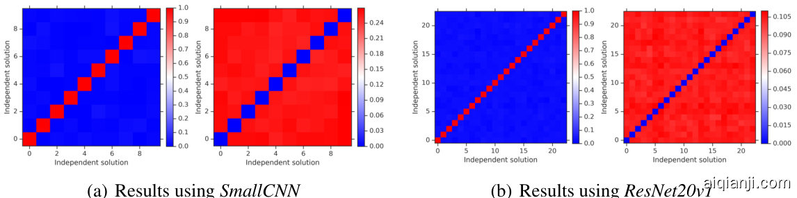
Figure 3: Results on CIFAR-10 using two different architectures. For each of these architectures, the left subplot shows the cosine similarity between different solutions in weight space, and the right subplot shows the fraction of labels on which the predictions from different solutions disagree. In general, the weight vectors from two different initialization s are essentially orthogonal, while their predictions are approximately as dissimilar as any other pair.

图 3: 在CIFAR-10数据集上使用两种不同架构的结果。对于每种架构，左子图显示权重空间中不同解之间的余弦相似度，右子图展示不同解预测结果出现分歧的标签比例。总体而言，两种不同初始化的权重向量基本正交，而它们的预测差异程度与任意其他配对近似。

4.2 Similarity of Functions Within Subspace from Each Trajectory and Across Trajectories

4.2 子空间内各轨迹间及跨轨迹的函数相似性

In addition to the checkpoints along a trajectory, we also construct subspaces based on each individual trajectory. Scalable variation al Bayesian methods typically approximate the distribution of weights along the training trajectory, hence visualizing the diversity of functions between the subspaces helps understand the difference between Bayesian neural networks and ensembles. We use a representative set of four subspace sampling methods: Monte Carlo dropout, a diagonal Gaussian approximation, a low-rank covariance matrix Gaussian approximation and a random subspace approximation. Unlike dropout and Gaussian approximations which assume a parametric form for the variation al posterior, the random subspace method explores all high-quality solutions within the subspace and hence could be thought of as a non-parametric variation al approximation to the posterior. Due to space constraints, we do not consider Markov Chain Monte Carlo (MCMC) methods in this work; Zhang et al. [2020] show that popular stochastic gradient MCMC (SGMCMC) methods may not explore multiple modes and propose cyclic SGMCMC. We compare diversity of random initialization and cyclic SGMCMC in Appendix C. In the descriptions of the methods, let $\theta_ {\mathrm{0}}$ be the optimized weight-space solution (the weights and biases of our trained neural net) around which we will construct the subspace.

除了轨迹上的检查点外，我们还基于每条独立轨迹构建子空间。可扩展的变分贝叶斯方法通常沿训练轨迹近似权重的分布，因此可视化子空间之间的函数多样性有助于理解贝叶斯神经网络与集成方法之间的差异。我们采用四种代表性的子空间采样方法：蒙特卡洛dropout、对角高斯近似、低秩协方差矩阵高斯近似和随机子空间近似。与假设变分后验具有参数形式的dropout和高斯近似不同，随机子空间方法探索子空间内所有高质量解，因此可视为后验的非参数变分近似。由于篇幅限制，本文未考虑马尔可夫链蒙特卡洛(MCMC)方法；Zhang等人[2020]表明流行的随机梯度MCMC(SGMCMC)方法可能无法探索多模态，并提出循环SGMCMC。我们在附录C中比较了随机初始化和循环SGMCMC的多样性。在方法描述中，设$\theta_ {\mathrm{0}}$为优化后的权重空间解(训练神经网络的权重和偏置)，我们将围绕该解构建子空间。

• Random subspace sampling: We start at an optimized solution $\pmb{\theta}_ {0}$ and choose a random direction $_ {v}$ in the weight space. We step in that direction by choosing different values of $t$ and looking at predictions at configurations $\mathbf{\nabla}\theta_ {0}+t\mathbf{v}$ . We repeat this for many random directions $_ {v}$ . • Dropout subspace: We start at an optimized solution $\pmb{\theta}_ {0}$ apply dropout with a randomly chosen $p_ {\mathrm{keep}}$ , evaluate predictions at $\mathrm{dropout}_ {p_ {\mathrm{keep}}}(\pmb{\theta}_ {0})$ and repeat this many times with different $p_ {\mathrm{keep}}$ . • Diagonal Gaussian subspace: We start at an optimized solution $\theta_ {\mathrm{0}}$ and look at the most recent iterations of training proceeding it. For each trainable parameter $\theta_ {i}$ , we calculate the mean $\mu_ {i}$ and standard deviation $\sigma_ {i}$ independently for each parameter, which corresponds to a diagonal covariance matrix. This is similar to SWAG-diagonal [Maddox et al., 2019]. To sample solutions from the subspace, we repeatedly draw samples where each parameter independently as $\theta_ {i}\sim\mathcal N(\mu_ {i},\sigma_ {i})$ . • Low-rank Gaussian subspace: We follow the same procedure as the diagonal Gaussian subspace above to compute the mean $\mu_ {i}$ for each trainable parameter. For the covariance, we use a rank $k$ approximation, by calculating the top $k$ principal components of the recent weight vectors ${\pmb{v}_ {i}\in\mathbb{R}^{\mathrm{params}}}_ {k}$ . We sample from a $k$ -dimensional normal distribution and obtain the weight configurations as $\begin{array}{r}{\pmb{\theta}\sim\pmb{\mu}+\sum_ {i}\mathcal{N}(0^{k},1^{k})\pmb{v}_ {i}}\end{array}$ . Throughout the text, we use the terms low-rank and PCA Gaussian interchange ably.

• 随机子空间采样：从优化解 $\pmb{\theta}_ {0}$ 出发，在权重空间中随机选取方向 $_ {v}$。通过选择不同的 $t$ 值，观察配置 $\mathbf{\nabla}\theta_ {0}+t\mathbf{v}$ 处的预测结果。对多个随机方向 $_ {v}$ 重复此过程。
• Dropout子空间：从优化解 $\pmb{\theta}_ {0}$ 出发，应用随机选择的 $p_ {\mathrm{keep}}$ 进行dropout，在 $\mathrm{dropout}_ {p_ {\mathrm{keep}}}(\pmb{\theta}_ {0})$ 处评估预测，并针对不同 $p_ {\mathrm{keep}}$ 多次重复。
• 对角高斯子空间：从优化解 $\theta_ {\mathrm{0}}$ 出发，考察其最近的训练迭代历史。对每个可训练参数 $\theta_ {i}$，独立计算均值 $\mu_ {i}$ 和标准差 $\sigma_ {i}$（对应对角协方差矩阵），类似SWAG-diagonal [Maddox et al., 2019]。通过独立采样 $\theta_ {i}\sim\mathcal N(\mu_ {i},\sigma_ {i})$ 从子空间中获取解。
• 低秩高斯子空间：沿用上述对角高斯子空间方法计算各参数的均值 $\mu_ {i}$。协方差采用秩$k$近似，通过计算近期权重向量 ${\pmb{v}_ {i}\in\mathbb{R}^{\mathrm{params}}}_ {k}$ 的top $k$主成分。从$k$维正态分布采样，获得权重配置 $\begin{array}{r}{\pmb{\theta}\sim\pmb{\mu}+\sum_ {i}\mathcal{N}(0^{k},1^{k})\pmb{v}_ {i}}\end{array}$。文中"低秩"与"PCA高斯"可互换使用。

Figure 4: Results using SmallCNN on CIFAR-10: t-SNE plots of validation set predictions for each trajectory along with four different subspace generation methods (showed by squares), in addition to 3 independently initialized and trained runs (different colors). As visible in the plot, the subspacesampled functions stay in the prediction-space neighborhood of the run around which they were constructed, demonstrating that truly different functions are not sampled.

图 4: 在CIFAR-10上使用SmallCNN的结果：验证集预测的t-SNE图，展示了每条轨迹以及四种不同的子空间生成方法（用方块表示），此外还有3个独立初始化和训练的运行（不同颜色）。从图中可以看出，子空间采样的函数始终围绕其构建的运行保持在预测空间邻域内，这表明并未采样到真正不同的函数。

Figure 4 shows that functions sampled from a subspace (denoted by colored squares) corresponding to a particular initialization, are much more similar to each other. While some subspaces are more diverse, they still do not overlap with functions from another randomly initialized trajectory.

图 4: 从对应特定初始化的子空间(以彩色方块表示)采样的函数彼此间相似度更高。虽然某些子空间更具多样性，但它们仍不会与另一随机初始化轨迹产生的函数重叠。

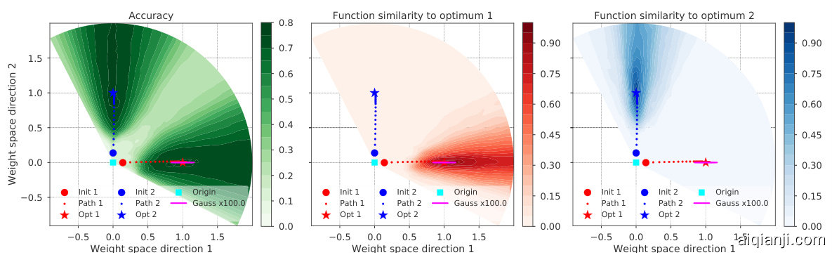
Figure 5: Results using MediumCNN on CIFAR-10: Radial loss landscape cut between the origin and two independent optima. Left plot shows accuracy of models along the paths of the two independent trajectories, and the middle and right plots show function space similarity to the two optima.

图 5: 在CIFAR-10上使用MediumCNN的结果：原点与两个独立最优解之间的径向损失景观切片。左图显示两个独立轨迹路径上模型的准确率，中间和右图显示与两个最优解在函数空间的相似性。

As additional evidence, Figure 5 provides a two-dimensional visualization of the radial landscape along the directions of two different optima. The 2D sections of the weight space visualized are defined by the origin (all weights are 0) and two independently initialized and trained optima. The weights of the two trajectories (shown in red and blue) are initialized using standard techniques and they increase radially with training due to their softmax cross-entropy loss. The left subplot shows that different randomly initialized trajectories eventually achieve similar accuracy. We also sample from a Gaussian subspace along trajectory 1 (shown in pink). The middle and the right subplots show function space similarity (defined as the fraction of points on which they agree on the class prediction) of the parameters along the path to optima 1 and 2. Solutions along each trajectory (and Gaussian subspace) are much more similar to their respective optima, which is consistent with the cosine similarity and t-SNE plots.

作为补充证据，图5展示了沿两个不同最优方向径向景观的二维可视化。所展示的权重空间二维截面由原点（所有权重为0）和两个独立初始化训练的最优点定义。两条轨迹（红色与蓝色所示）的权重采用标准技术初始化，并因其softmax交叉熵损失而在训练过程中径向增长。左子图显示不同随机初始化轨迹最终达到相近的准确率。我们还沿轨迹1（粉色所示）在高斯子空间中进行采样。中间与右侧子图展示了参数在通往最优1和2路径上的函数空间相似性（定义为类别预测一致点的比例）。每条轨迹（及高斯子空间）上的解与其对应最优解的相似度显著更高，这与余弦相似度和t-SNE图的结果一致。

4.3 Diversity versus Accuracy plots

4.3 多样性 vs 准确率曲线图

To illustrate the difference in another fashion, we sample functions from a single subspace and plot accuracy versus diversity, as measured by disagreement between predictions from the baseline solution. From a bias-variance trade-off perspective, we require a procedure to produce functions that are accurate (which leads to low bias by aggregation) as well as de-correlated (which leads to lower variance by aggregation). Hence, the diversity vs accuracy plot allows us to visualize the trade-off that can be achieved by subspace sampling methods versus deep ensembles.

为了以另一种方式说明差异，我们从单一子空间中采样函数，并绘制准确性与多样性之间的关系图，其中多样性通过基线解决方案预测之间的分歧来衡量。从偏差-方差权衡的角度来看，我们需要一种方法生成既准确（通过聚合降低偏差）又去相关（通过聚合降低方差）的函数。因此，多样性-准确性关系图使我们能够直观比较子空间采样方法与深度集成方法所能实现的权衡效果。

The diversity score quantifies the difference of two functions (a base solution and a sampled one), by measuring fraction of datapoints on which their predictions differ. We chose this approach due to its simplicity; we also computed the KL-divergence and other distances between the output probability distributions, leading to equivalent conclusions. Let $d_ {\mathrm{diff}}$ denote the fraction of predictions on which the two functions differ. It is 0 when the two functions make identical class predictions, and 1 when they differ on every single example. To account for the fact that the lower the accuracy of a function, the higher its potential $d_ {\mathrm{diff}}$ due to the possibility of the wrong answers being random and uncorrelated between the two functions, we normalize this by $(1-a)$ , where $a$ is the accuracy of the sampled solution. We also derive idealized lower and upper limits of these curves (showed in dashed lines) by perturbing the reference solution’s predictions (lower limit) and completely random predictions at a given accuracy (upper limit), see Appendix D for a discussion.

多样性分数通过衡量两个函数（一个基础解和一个采样解）预测结果不同的数据点比例，来量化它们之间的差异。我们选择这种方法是因为其简单性；同时我们还计算了输出概率分布之间的KL散度和其他距离，得出了等效的结论。设$d_ {\mathrm{diff}}$表示两个函数预测结果不同的比例。当两个函数做出完全相同的类别预测时为0，当它们在所有样本上都不同时为1。考虑到函数准确率越低，由于错误答案可能在两个函数间随机且不相关，其潜在的$d_ {\mathrm{diff}}$会越高，我们通过$(1-a)$对其进行归一化，其中$a$是采样解的准确率。我们还通过扰动参考解的预测（下限）和在给定准确率下完全随机的预测（上限），推导出这些曲线的理想化上下限（以虚线显示），具体讨论见附录D。

Figure 6: Diversity versus accuracy plots for 3 models trained on CIFAR-10: SmallCNN, MediumCNN and a ResNet20v1. Independently initialized and optimized solutions (red stars) achieve better diversity vs accuracy trade-off than the four different subspace sampling methods.

图 6: CIFAR-10数据集上训练的3个模型( SmallCNN、MediumCNN和ResNet20v1 )的多样性-准确率关系图。独立初始化和优化的解决方案(红星)比四种不同的子空间采样方法实现了更好的多样性-准确率权衡。

Figure 6 shows the results on CIFAR-10. Comparing these subspace points (colored dots) to the baseline optima (green star) and the optima from different random initialization s (denoted by red stars), we observe that random initialization s are much more effective at sampling diverse and accurate solutions, than subspace based methods constructed out of a single trajectory. The results are consistent across different architectures and datasets. Figure 7 shows results on CIFAR-100 and ImageNet. We observe that solutions obtained by subspace sampling methods have a worse trade off between accuracy and prediction diversity, compared to independently initialized and trained optima. Interestingly, the separation between the subspace sampling methods and independent optima in the diversity–accuracy plane gets more pronounced the more difficult the problem and the more powerful the network.

图6展示了CIFAR-10上的实验结果。将这些子空间采样点(彩色圆点)与基线最优解(绿色星标)及不同随机初始化得到的最优解(红色星标)对比时，我们发现随机初始化在获取多样且精确解方面，远比基于单条轨迹构建的子空间方法更有效。该结论在不同架构和数据集上保持一致性。图7呈现了CIFAR-100和ImageNet的实验结果。我们观察到，相较于独立初始化训练得到的最优解，子空间采样方法获得的解在准确率与预测多样性之间呈现更差的权衡关系。值得注意的是，随着任务难度提升和网络能力增强，子空间采样方法与独立最优解在多样性-准确率平面上的分离现象会愈发显著。

(a) ResNet20v1 trained on CIFAR-100. (b) ResNet50v2 trained on ImageNet. igure 7: Diversity vs. accuracy plots for ResNet20v1 on CIFAR-100, and ResNet50v2 on ImageNe

(a) 在CIFAR-100上训练的ResNet20v1。(b) 在ImageNet上训练的ResNet50v2。
图7: ResNet20v1在CIFAR-100上及ResNet50v2在ImageNet上的多样性与准确率关系图

5 Evaluating the Relative Effects of Ensembling versus Subspace Methods

5 评估集成方法与子空间方法的相对效果

Our hypothesis in Figure 1 and the empirical observations in the previous section suggest that subspace-based methods and ensembling should provide complementary benefits in terms of uncertainty and accuracy. Since our goal is not to propose a new method, but to carefully test this hypothesis, we evaluate the performance of the following four variants for controlled comparison:

图 1 中的假设及前文实证观察表明，基于子空间的方法和集成技术应在不确定性与准确性方面形成互补优势。由于我们的目标并非提出新方法，而是严谨验证该假设，因此通过以下四种变体进行对照实验评估：

To maintain the accuracy of random samples at a reasonable level for fair comparison, we reject the sample if validation accuracy is below 0.65. For the CIFAR-10 experiment, we use a rank-4 approximation of the random samples using PCA. Note that diagonal Gaussian, low-rank Gaussian and random subspace sampling methods to approximate each mode of the posterior leads to an increase in the number of parameters required for each mode. However, using just the mean weights for each mode would not cause such an increase. Izmailov et al. [2018] proposed stochastic weight averaging (SWA) for better generalization. One could also compute an (exponential moving) average of the weights along the trajectory, inspired by Polyak-Ruppert averaging in convex optimization, (see also [Mandt et al., 2017] for a Bayesian view on iterate averaging). As weight averaging (WA) has been already studied by Izmailov et al. [2018], we do not discuss it in detail. Our goal is to test if WA finds a better point estimate within each mode (see cartoon illustration in Figure 1) and provides complementary benefits to ensembling over random initialization. In our experiments, we use WA on the last few epochs which corresponds to using just the mean of the parameters within each mode.

为了将随机样本的准确率维持在合理水平以确保公平比较，若验证准确率低于0.65，我们将拒绝该样本。在CIFAR-10实验中，我们使用PCA对随机样本进行秩4近似。需要注意的是，对角高斯、低秩高斯和随机子空间采样等近似后验各模态的方法会导致每个模态所需的参数数量增加。然而，若仅使用各模态的权重均值则不会产生此类增加。Izmailov等[2018]提出了随机权重平均(SWA)以提升泛化能力。受凸优化中Polyak-Ruppert平均的启发，也可以沿轨迹计算权重的(指数移动)平均值(另见[Mandt等，2017]关于迭代平均的贝叶斯观点)。由于权重平均(WA)已被Izmailov等[2018]研究过，本文不再详细讨论。我们的目标是验证WA能否在各模态内找到更优的点估计(见图1的示意图)，并为随机初始化集成提供互补优势。实验中，我们对最后几个周期应用WA，这相当于仅使用各模态内参数的均值。

Figure 8 shows the results on CIFAR-10. The results validate our hypothesis that (i) subspace sampling and ensembling provide complementary benefits, and (ii) the relative benefits of ensembling are higher as it averages predictions over more diverse solutions.

图 8: 展示了在 CIFAR-10 上的实验结果。结果验证了我们的假设：(i) 子空间采样 (subspace sampling) 和集成 (ensembling) 能带来互补优势，(ii) 当集成对更多样化的解决方案进行预测平均时，其相对收益更高。

Figure 8: Results using MediumCNN on CIFAR-10 showing the complementary benefits of ensemble and subspace methods as a function of ensemble size. We used 10 samples for each subspace method.

图 8: 在CIFAR-10数据集上使用MediumCNN的实验结果，展示了集成方法和子空间方法随着集成规模变化的互补优势。每个子空间方法使用了10个样本。

Effect of function space diversity on dataset shift We test the same hypothesis under dataset shift [Ovadia et al., 2019, Hendrycks and Dietterich, 2019]. Left and middle subplots of Figure 9 show accuracy and Brier score on the CIFAR-10-C benchmark. We observe again that ensembles and subspace sampling methods provide complementary benefits.

函数空间多样性对数据集偏移的影响
我们在数据集偏移 [Ovadia et al., 2019, Hendrycks and Dietterich, 2019] 条件下测试了相同假设。图 9 左右子图分别展示了 CIFAR-10-C 基准测试中的准确率和 Brier 分数。再次观察到集成方法与子空间采样方法能提供互补优势。

The diversity versus accuracy plot compares diversity to a reference solution, but it is also important to also look at the diversity between multiple samples of the same method, as this will effectively determine the efficiency of the method in terms of the bias-variance trade-off. Function space diversity is particularly important to avoid overconfident predictions under dataset shift, as averaging over similar functions would not reduce over confidence. To visualize this, we draw 5 samples of each method and compute the average Jensen-Shannon divergence between their predictions, defined asKL(p((g)where KL denotes theKulback-Leb ler div r gence and $\begin{array}{r}{\bar{p}(y|\pmb{x})=(1/\bar{M})\sum_ {m}p_ {\pmb{\theta}_ {m}}(y|\pmb{x})}\end{array}$ . Right subplot of Figure 9 shows the results on CIFAR-10-C for increasing corrup tion intensity. We observe that Jensen-Shannon divergence is the highest between independent random initialization s, and lower for subspace sampling methods; the difference is higher under dataset shift, which explains the findings of Ovadia et al. [2019] that deep ensembles outperform other methods under dataset shift. We also observe similar trends when testing on an OOD dataset such as SVHN: JS divergence is 0.384 for independent runs, 0.153 for within-trajectory, 0.155 for random sampling, 0.087 for rank-5 PCA Gaussian and 0.034 for diagonal Gaussian.

多样性与准确率对比图将多样性与参考解进行比较，但同样重要的是观察同一方法多个样本间的多样性，因为这能有效反映该方法在偏差-方差权衡中的效率。函数空间多样性对于避免数据集偏移下的过度自信预测尤为关键，因为对相似函数取平均并不能降低过度自信。为直观展示这一点，我们为每种方法抽取5个样本，计算其预测间的平均Jensen-Shannon散度，定义为KL(p(g))，其中KL表示Kullback-Leibler散度，且$\begin{array}{r}{\bar{p}(y|\pmb{x})=(1/\bar{M})\sum_ {m}p_ {\pmb{\theta}_ {m}}(y|\pmb{x})}\end{array}$。图9右侧子图展示了CIFAR-10-C数据集上随着损坏强度增加的结果。我们观察到：独立随机初始化间的Jensen-Shannon散度最高，子空间采样方法较低；这种差异在数据集偏移下更为显著，这解释了Ovadia等[2019]的发现——深度集成在数据集偏移下优于其他方法。在SVHN等OOD数据集测试中我们也观察到相似趋势：独立运行的JS散度为0.384，轨迹内采样为0.153，随机采样为0.155，秩5PCA高斯为0.087，对角高斯为0.034。

Figure 9: Results using MediumCNN on CIFAR-10-C for varying levels of corruption intensity. Left plot shows accuracy, medium plot shows Brier score and right plot shows Jensen-Shannon divergence.

图 9: 在CIFAR-10-C数据集上使用MediumCNN模型对不同破坏强度的结果。左图显示准确率，中图显示Brier分数，右图显示Jensen-Shannon散度。

Results on ImageNet To illustrate the effect on another challenging dataset, we repeat these experiments on ImageNet [Deng et al., 2009] using ResNet50v2 architecture. Due to computational constraints, we do not evaluate PCA subspace on ImageNet. Figure 10 shows results on ImageNet test set (zero corruption intensity) and ImageNet-C for increasing corruption intensities. Similar to CIFAR-10, random subspace performs best within subspace sampling methods, and provides complementary benefits to random initialization. We empirically observed that the relative gains of WA (or subspace sampling) are smaller when the individual models converge to a better optima within each mode. Carefully choosing which points to average, e.g. using cyclic learning rate as done in fast geometric ensembling [Garipov et al., 2018] can yield further benefits.

ImageNet上的结果
为展示在另一个挑战性数据集上的效果，我们使用ResNet50v2架构在ImageNet [Deng et al., 2009] 上重复了这些实验。由于计算资源限制，我们未在ImageNet上评估PCA子空间方法。图10展示了ImageNet测试集（零损坏强度）和ImageNet-C随损坏强度增加的结果。与CIFAR-10类似，在子空间采样方法中随机子空间表现最佳，并为随机初始化提供了互补优势。我们通过实验观察到，当单个模型在每个模态内收敛到更优解时，权重平均 (WA) 或子空间采样的相对收益会减小。谨慎选择平均点（例如采用快速几何集成 [Garipov et al., 2018] 中的循环学习率策略）可带来额外提升。

Figure 10: Results using ResNet50v2 on ImageNet test and ImageNet-C for varying corruptions.

图 10: 使用 ResNet50v2 在 ImageNet 测试集和 ImageNet-C 上针对不同损坏类型的结果。

6 Discussion

6 讨论

Through extensive experiments, we show that trajectories of randomly initialized neural networks explore different modes in function space, which explains why deep ensembles trained with just random initialization s work well in practice. Subspace sampling methods such as weight averaging, Monte Carlo dropout, and various versions of local Gaussian approximations, sample functions that might lie relatively far from the starting point in the weight space, however, they remain similar in function space, giving rise to an insufficiently diverse set of predictions. Using the concept of the diversity–accuracy plane, we demonstrate empirically that current variation al Bayesian methods do not reach the trade-off between diversity and accuracy achieved by independently trained models. There are several interesting directions for future research: understanding the role of random initialization on training dynamics (see Appendix B for a preliminary investigation), exploring methods which achieve higher diversity than deep ensembles (e.g. through explicit de correlation), and developing parameter-efficient methods (e.g. implicit ensembles or Bayesian deep learning algorithms) that achieve better diversity–accuracy trade-off than deep ensembles.

通过大量实验，我们发现随机初始化神经网络的轨迹会在函数空间中探索不同模式，这解释了为何仅通过随机初始化训练的深度集成方法在实践中表现良好。权重平均、蒙特卡洛dropout以及各类局部高斯近似等子空间采样方法，虽然能采样到权重空间中距离起点较远的函数，但这些函数在函数空间中仍保持相似性，导致预测集缺乏足够多样性。借助多样性-准确性平面的概念，我们通过实证表明当前变分贝叶斯方法未能达到独立训练模型所实现的多样性-准确性平衡。未来研究有几个值得探索的方向：理解随机初始化对训练动态的影响（初步分析见附录B）、开发比深度集成具有更高多样性的方法（例如通过显式去相关）、以及设计参数效率更高的方法（如隐式集成或贝叶斯深度学习算法）以实现优于深度集成的多样性-准确性权衡。

Alex Krizhevsky. Learning multiple layers of features from tiny images. 2009.

Alex Krizhevsky. 从小图像中学习多层特征. 2009.

Supplementary Material

补充材料

A Identical loss does not imply identical functions in prediction space

相同的损失并不意味着预测空间中功能相同

To make our paper self-contained, we review the literature on loss surfaces and mode connectivity [Garipov et al., 2018, Draxler et al., 2018, Fort and J as tr zeb ski, 2019]. We provide visualization s of the loss surface which confirm the findings of prior work as well as complement them. Figure S1 shows the radial loss landscape (train as well as the validation set) along the directions of two different optima. The left subplot shows that different trajectories achieve similar values of the loss, and the right subplot shows the similarity of these functions to their respective optima (in particular the fraction of labels predicted on which they differ divided by their error rate). While the loss values from different optima are similar, the functions are different, which confirms that random initialization leads to different modes in function space.

为使本文自成体系，我们回顾了关于损失曲面和模态连通性的文献 [Garipov et al., 2018, Draxler et al., 2018, Fort and Jastrzebski, 2019]。我们提供了损失曲面的可视化结果，这些结果既验证了先前工作的发现，又对其进行了补充。图 S1 展示了沿两个不同最优方向上的径向损失景观（训练集和验证集）。左子图显示不同轨迹实现了相似的损失值，右子图则展示了这些函数与其各自最优解的相似性（具体表现为预测标签差异占比除以错误率）。虽然不同最优解的损失值相近，但这些函数本身存在差异，这证实了随机初始化会导致函数空间中出现不同模态。

(a) Accuracy along the radial loss-landscape cut (b) Function-space similarity

图 1:
(a) 径向损失景观切片的准确度 (b) 函数空间相似性

Next, we construct a low-loss tunnel between different optima using the procedure proposed by Fort and J as tr zeb ski [2019], which is a simplification of the procedures proposed in Garipov et al. [2018] and Draxler et al. [2018]. As shown in Figure S2(a), we start at the linear interpolation point (denoted by the black line) and reach the closest point on the manifold by minimizing the training loss. The minima of the training loss are denoted by the yellow line in the manifolds. Figure S2(b) confirms that the tunnel is indeed low-loss. This also confirms the findings of [Garipov et al., 2018, Fort and J as tr zeb ski, 2019] that while solutions along the tunnel have similar loss, they are dissimilar in function space.

接下来，我们采用 Fort 和 Jastrzębski [2019] 提出的方法在不同最优解之间构建低损耗隧道，该方法是对 Garipov 等人 [2018] 和 Draxler 等人 [2018] 所提流程的简化。如图 S2(a) 所示，我们从线性插值点（黑色线段表示）出发，通过最小化训练损失到达流形上的最近点。训练损失的极小值在流形中用黄色线段标示。图 S2(b) 证实该隧道确实具有低损耗特性，这也验证了 [Garipov 等人, 2018, Fort 和 Jastrzębski, 2019] 的发现：虽然隧道沿线解具有相近的损失值，但它们在函数空间中存在显著差异。

Figure S1: Results using MediumCNN on CIFAR-10: Radial loss landscape cut between the origin and two independent optima and the predictions of models on the same plane. Figure S2: Left: Cartoon illustration showing linear connector (black) along with the optimized connector which lies on the manifold of low loss solutions. Right: The loss and accuracy in between two independent optima on a linear path and an optimized path in the weight space.

图 S1: 在CIFAR-10数据集上使用MediumCNN的结果: 原点与两个独立最优解之间的径向损失景观切面及模型在同一平面上的预测。图 S2: 左: 示意图展示线性连接路径 (黑色) 与位于低损失解流形上的优化连接路径。右: 权重空间中线性路径和优化路径上两个独立最优解之间的损失与准确率变化。

In order to visualize the 2-dimensional cut through the loss landscape and the associated predictions along a curved low-loss path, we divide the path into linear segments, and compute the loss and prediction similarities on a triangle given by this segment on one side and the origin of the weight space on the other. We perform this operation on each of the linear segments from which the low-loss path is constructed, and place them next to each other for visualization. Figure S3 visualizes the loss along the manifold, as well as the similarity to the original optima. Note that the regions between radial yellow lines consist of segments, and we stitch these segments together in Figure S3. The accuracy plots show that as we traverse along the low-loss tunnel, the accuracy remains fairly constant as expected. However, the prediction similarity plot shows that the low-loss tunnel does not correspond to similar solutions in function space. What it shows is that while the modes are connected in terms of accuracy/loss, their functional forms remain distinct and they do not collapse into a single mode.

为了可视化损失景观的二维截面以及沿弯曲低损失路径的预测结果，我们将路径划分为线性段，并在由该段与权重空间原点构成的三角形上计算损失和预测相似度。我们对构成低损失路径的每个线性段执行此操作，并将它们并排排列以进行可视化。图 S3 展示了沿流形的损失情况以及与原始最优解的相似度。请注意，黄色径向线之间的区域由多个线段组成，我们在图 S3 中将它们拼接在一起。准确率曲线表明，随着我们在低损失通道中移动，准确率如预期保持相对稳定。然而，预测相似度图显示，低损失通道并不对应函数空间中的相似解。这表明虽然这些模态在准确率/损失方面是连通的，但它们的函数形式仍然不同，并未坍缩为单一模态。

Figure S3: Results using MediumCNN on CIFAR-10: Radial loss landscape cut between the origin and two independent optima along an optimized low-loss connector and function space similarity (agreement of predictions) to the two optima along the same planes.

图 S3: 在CIFAR-10数据集上使用MediumCNN的结果：沿优化后的低损失连接器在原点与两个独立最优解之间切割的径向损失景观，以及沿相同平面对两个最优解的函数空间相似性(预测一致性)。

B Effect of randomness: random initialization versus random shuffling

B 随机性影响：随机初始化与随机洗牌对比

Random seed affects both initial parameter values as well the order of shuffling of data points. We run experiments to decouple the effect of random initialization and shuffling; Figure S4 shows the results. We observe that both of them provide complementary sources of randomness, with random initialization being the dominant of the two. As expected, random mini-batch shuffling adds more randomness at higher learning rates due to gradient noise.

随机种子既影响初始参数值，也影响数据点的洗牌顺序。我们通过实验分离随机初始化和洗牌顺序的影响；图 S4 展示了结果。观察到二者提供互补的随机性来源，其中随机初始化起主导作用。正如预期，由于梯度噪声的存在，随机小批量洗牌在较高学习率下会引入更多随机性。

Figure S4: The effect of random initialization s and random training batches on the diversity of predictions. For runs on a GPU, the same initialization and the same training batches (red) do not lead to the exact same predictions. On a TPU, such runs always learn the same function and have therefore 0 diversity of predictions.

图 S4: 随机初始化参数s和随机训练批次对预测多样性的影响。在GPU上运行时，相同的初始化和相同的训练批次（红色）不会导致完全相同的预测结果。而在TPU上，此类运行总会学习到相同的函数，因此预测多样性为0。

C Comparison to cSG-MCMC

C 与 cSG-MCMC 的对比

Zhang et al. [2020] show that vanilla stochastic gradient Markov Chain Monte Carlo (SGMCMC) methods do not explore multiple modes in the posterior and instead propose cyclic stochastic gradient MCMC (cSG-MCMC) to achieve that. We ran a suite of verification experiments to determine whether the diversity of functions found using the proposed cSG-MCMC algorithm matches that of independently randomly initialized and trained models.

张等人[20]研究表明，传统随机梯度马尔可夫链蒙特卡洛(SGMCMC)方法无法探索后验分布中的多模态，因此提出循环随机梯度MCMC(cSG-MCMC)来实现这一目标。我们进行了一系列验证实验，以确定使用cSG-MCMC算法发现的函数多样性是否与独立随机初始化和训练模型的结果相匹配。

We used the code published by the authors Zhang et al. [2020] 5 to match exactly the setup of their paper. We ran cSG-MCMC from 3 random initialization s, each for a total of 150 epochs amounting to 3 cycles of the 50 epoch period learning rate schedule. We used a ResNet-18 and ran experiments on both CIFAR-10 and CIFAR-100. We measured the function diversity between a) independently initialized and trained runs, and b) between different cyclic learning rate periods within the same run of the cSG-MCMC. The latter (b) should be comparable to the former (a) if cSG-MCMC was as successful as vanilla deep ensembles at producing diverse functions. We show that both for CIFAR-10 and CIFAR-100, vanilla ensembles generate statistically significantly more diverse sets of functions than cSG-MCMC, as shown in Figure C. While cSG-MCMC is doing well in absolute terms, the shared initialization for cSG-MCMC training seems to lead to lower diversity than deep ensembles with multiple random initialization s. Another difference between the methods is that individual members of deep ensemble can be trained in parallel unlike cSG-MCMC.

我们采用了Zhang等人[2020]5公开的代码，以精确复现其论文中的实验设置。cSG-MCMC从3个随机初始化点开始运行，每个点进行150个周期（即50周期学习率调度表的3轮循环）。实验使用ResNet-18架构，并在CIFAR-10和CIFAR-100数据集上进行。我们测量了以下两种情况下的函数多样性：(a) 独立初始化训练的运行结果，(b) 同一cSG-MCMC运行中不同周期学习率阶段的结果。若cSG-MCMC能像传统深度集成方法那样有效生成多样化函数，则后者(b)的多样性应与前者(a)相当。如图C所示，在CIFAR-10和CIFAR-100上，传统集成方法产生的函数集在统计显著性上比cSG-MCMC更具多样性。尽管cSG-MCMC的绝对表现良好，但其共享初始化的训练方式似乎导致其多样性低于采用多重随机初始化的深度集成方法。另一个区别在于：深度集成的单个成员可并行训练，而cSG-MCMC则不具备这一特性。

Figure S5: Comparison of function space diversities between the cSG-MCMC (blue) and deep ensembles (red). The left panel shows the experiments with ResNet-18 on CIFAR-10 and the right panel shows the experiments on CIFAR-100. In both cases, deep ensembles produced a statistically significantly more diverse set of functions than cSG-MCMC as measured by our function diversity metric. The plots show the mean and $1\sigma$ confidence intervals based on 4 experiments each.

图 S5: cSG-MCMC (蓝色) 与深度集成 (红色) 在函数空间多样性上的对比。左图展示 ResNet-18 在 CIFAR-10 上的实验结果，右图展示 CIFAR-100 上的实验结果。根据我们的函数多样性指标测量，两种情况下深度集成产生的函数集在统计显著性上比 cSG-MCMC 更具多样性。图中显示基于4次实验的均值及 $1\sigma$ 置信区间。

D Modeling the accuracy – diversity trade off

建模准确性与多样性的权衡

In our diversity–accuracy plots (e.g. Figure 6), subspace samples trade off their accuracy for diversity in a characteristic way. To better understand where this relationship comes from, we derive several limiting curves based on an idealized model. We also propose a 1-parameter family of functions that provide a surprisingly good fit (given the simplicity of the model) to our observation, as shown in Figure S6.

在我们的多样性-准确率关系图(例如图6)中，子空间样本会以特定方式牺牲准确率来换取多样性。为了更好地理解这种关系的来源，我们基于理想化模型推导出若干极限曲线。我们还提出一个单参数函数族，该函数族(考虑到模型的简洁性)能惊人地拟合我们的观测结果，如图S6所示。

We will be studying a pair of functions in a $C$ -class problem: the reference solution $f^{* }$ of accuracy $a^{*}$ , and another function $f$ of accuracy $a$ .

我们将研究一个$C$类问题中的一对函数：准确率为$a^{* }$的参考解$f^{*}$，以及准确率为$a$的另一个函数$f$。

D.1 Uncorrelated predictions: the best case

D.1 不相关预测：最佳情况

The best case scenario is when the predicted labels are uncorrelated with the reference solution’s labels. On a particular example, the probability that the reference solution got it correctly is $a^{* }$ , and the probability that the new solution got it correctly is $a$ . On those examples, the predictions do not differ since they both have to be equal to the ground truth label. The probability that the reference solution is correct on an example while the new solution is wrong is $a^{* }(1-a)$ . The probability that the reference solution is wrong on an example while the new solution is correct is $(1-a^{* })a$ . On the examples where both solutions are wrong (probability $(1-a^{*})(1-a))$ , there are two cases:

最佳情况是预测标签与参考解的标签不相关。在特定示例中，参考解正确的概率为 $a^{* }$，新解正确的概率为 $a$。在这些示例中，预测结果不会不同，因为它们都必须等于真实标签。参考解正确而新解错误的概率为 $a^{* }(1-a)$。参考解错误而新解正确的概率为 $(1-a^{* })a$。在两者都错误的示例中（概率 $(1-a^{*})(1-a))$），存在两种情况：

Only case 2 contributes to the fraction of labels on which they disagree. Hence we end up with

只有情况2会导致标签不一致的比例。因此我们最终得到

$$
d_ {\mathrm{diff}}(a;a^{* },C)=(1-a^{* })a+(1-a)a^{* }+(1-a^{*})(1-a)\frac{C-2}{C-1}.
$$

This curve corresponds to the upper limit in Figure 6. The diversity reached in practice is not as high as the theoretical optimum even for the independently initialized and optimized solutions, which provides scope for future work.

这条曲线对应图6中的上限。在实践中，即使是独立初始化和优化的解决方案，所达到的多样性也不如理论最优值高，这为未来的工作提供了空间。

D.2 Correlated predictions: the lower limit

D.2 相关预测：下限

By inspecting Figure 6 as well as a priori, we would expect a function $f$ close to the reference function $f^{* } $ in the weight space to have correlated predictions. We can model this by imagining that the predictions of $f$ are just the predictions of the reference solution $f^{* }$ perturbed by perturbations of a particular strength (which we vary). Let the probability of a label changing be $p$ . We will consider four cases:

通过观察图6以及先验知识，我们可以预期权重空间中接近参考函数$f^{* }$的函数$f$会具有相关性预测。这一现象可以通过设想$f$的预测仅是参考解$f^{*}$的预测受到特定强度(可调节)扰动来建模。设标签变化的概率为$p$。我们将考虑以下四种情况:

The resulting accuracy $a(p)$ obtains a contribution $a^{* }(1-p)$ from case 1) and a contribution $(1-a^{* })p$ with probability $1/(C-\mathrm{{1})}$ from case 4). Therefore $a(p)=a^{* }(1-p)+p(1-a^{* })/(C-1)$ . Inverting this relationship, we get $p(a)=(C-1)(a^{* }-a)/(C a^{*}-1)$ . The fraction of labels on which the solutions disagree is simply $p$ by our definition of $p$ , and therefore

最终准确率 $a(p)$ 由情况1)贡献 $a^{* }(1-p)$，由情况4)以概率 $1/(C-\mathrm{{1})}$ 贡献 $(1-a^{* })p$。因此 $a(p)=a^{* }(1-p)+p(1-a^{* })/(C-1)$。逆推该关系可得 $p(a)=(C-1)(a^{* }-a)/(C a^{*}-1)$。根据我们对 $p$ 的定义，解不一致的标签比例即为 $p$，因此

$$
d_ {\mathrm{diff}}(a;a^{* },C)=\frac{(C-1)(a^{* }-a)}{C a^{*}-1}.
$$

This curve corresponds to the lower limit in Figure 6.

该曲线对应图6中的下限。

D.3 Correlated predictions: 1-parameter family

D.3 相关预测：单参数族

Figure S6: Theoretical model of the accuracy-diversity trade-off and a comparison to ResNet20v1 on CIFAR-100. The left panel shows accuracy-diversity trade offs modelled by a 1-parameter family of functions specified by an exponent $e$ . The right panel shows real subspace samples for a ResNet20v1 trained on CIFAR-100 and the best fitting function with $e=0.22$ .

图 S6: 准确率-多样性权衡的理论模型及与CIFAR-100上ResNet20v1的对比。左图展示了由指数$e$定义的1参数函数族建模的准确率-多样性权衡曲线。右图展示了在CIFAR-100上训练的ResNet20v1真实子空间样本及最优拟合函数($e=0.22$)。

We can improve upon this model by considering two separate probabilities of labels flipping: $p_ {+}$ , which is the probability that a correctly labelled example will flip, and $p_ {-}$ , corresponding to the probability that a wrongly labelled example will flip its label. By repeating the previous analysis, we obtain

我们可以通过考虑标签翻转的两个独立概率来改进这个模型：$p_ {+}$，即正确标记的样本发生翻转的概率，以及$p_ {-}$，对应错误标记的样本翻转其标签的概率。重复之前的分析后，我们得到

$$
d_ {\mathrm{diff}}(p_ {+},p_ {-};a^{* },C)=a^{* }(1-p_ {+})+(1-a^{* })p_ {-}\frac{1}{C-1},
$$

$$
d_ {\mathrm{diff}}(p_ {+},p_ {-};a^{* },C)=a^{* }(1-p_ {+})+(1-a^{*})p_ {-}\frac{1}{C-1},
$$

and

和

$$
a(p_ {+},p_ {-};a^{* },C)=a^{* }p_ {+}+(1-a^{*})p_ {-}.
$$

The previously derived lower limit corresponds to the case $p_ {+}=p_ {-}=p\in[0,1]$ , where the probability of flipping the correct labels is the same as the probability of flipping the incorrect labels. The absolute worst case scenario would correspond to the situation where $p_ {+}=p$ , while $p_ {-}=0$ , i.e. only the correctly labelled examples flip.

先前推导出的下限对应于 $p_ {+}=p_ {-}=p\in[0,1]$ 的情况，即正确标签被翻转的概率与错误标签被翻转的概率相同。绝对最坏情况将对应于 $p_ {+}=p$ 而 $p_ {-}=0$ 的情形，即只有正确标注的样本会发生翻转。

We found that tying the two probabilities together via an exponent $e$ as $p_ {+}=p$ and $p_ {-}=p^{e}=p_ {+}^{e}$ generates a realistic looking trade off between accuracy and diversity. We show the resulting functions for several values of $e$ in Figure S6. For $e<1$ , the chance of flipping the wrong label is larger than that of the correct label, simulating a robustness of the learned solution to perturbations. We found the closest match to our data provided by $e=0.22$ .

我们发现通过指数 $e$ 将两个概率关联为 $p_ {+}=p$ 和 $p_ {-}=p^{e}=p_ {+}^{e}$ 时，能在准确性与多样性之间形成合理的权衡关系。图 S6 展示了不同 $e$ 值对应的函数曲线。当 $e<1$ 时，错误标签翻转的概率大于正确标签，这模拟了学习方案对扰动的鲁棒性。实验数据显示 $e=0.22$ 时与我们的数据吻合度最高。

[论文翻译]Deep Ensembles: 从损失函数视角解读

原文地址：https://arxiv.org/pdf/1912.02757v2