Rethinking Recurrent Neural Networks and Other Improvements for Image Classification
重新思考循环神经网络及其他图像分类改进方案
Abstract—Over the long history of machine learning, which dates back several decades, recurrent neural networks (RNNs) have been used mainly for sequential data and time series and generally with 1D information. Even in some rare studies on 2D images, these networks are used merely to learn and generate data sequentially rather than for image recognition tasks. In this study, we propose integrating an RNN as an additional layer when designing image recognition models. We also develop end-to-end multimodel ensembles that produce expert predictions using several models. In addition, we extend the training strategy so that our model performs comparably to leading models and can even match the state-of-the-art models on several challenging datasets (e.g., SVHN (0.99), Cifar-100 (0.9027) and Cifar-10 (0.9852)). Moreover, our model sets a new record on the Surrey dataset (0.949). The source code of the methods provided in this article is available at https://github.com/leonlha/e2e-3m and http://nguyen hu up hong.me.
摘要—在长达数十年的机器学习发展史中,循环神经网络(RNN)主要被用于处理序列数据和时间序列,且通常针对一维信息。即使在少数关于二维图像的研究中,这些网络也仅用于顺序学习和生成数据,而非图像识别任务。本研究提出在设计图像识别模型时将RNN作为附加层进行集成,并开发了端到端多模型集成方法,通过多个模型生成专家预测。此外,我们扩展了训练策略,使得我们的模型性能可与领先模型相媲美,在多个具有挑战性的数据集(如SVHN(0.99)、Cifar-100(0.9027)和Cifar-10(0.9852))上甚至能达到最先进模型的水平。更重要的是,我们的模型在Surrey数据集上创造了新纪录(0.949)。本文提供的方法源代码可见于https://github.com/leonlha/e2e-3m和http://nguyen hu up hong.me。
1 INTRODUCTION
1 引言
Recently, the image recognition task has been transformed by the availability of high-performance computing hardware—particularly modern graphical processing units (GPUs) and large-scale datasets. The early designs of convolutional neural networks (ConvNets) in the 1990s were shallow and included only a few layers; however, as the everincreasing volume of image data with higher resolutions required a concomitant increase in computing power, the field has evolved; modern ConvNets have deeper and wider layers with improved efficiency and accuracy [1], [2], [3], [4], [5], [6], [7]. The later developments involved a balancing act among network depth, width and image resolution [8] and determining appropriate augmentation policies [9].
近年来,图像识别任务因高性能计算硬件(特别是现代图形处理器(GPU))和大规模数据集的普及而发生变革。20世纪90年代早期的卷积神经网络(ConvNet)设计较浅,仅包含少数几层;但随着高分辨率图像数据量的持续增长对计算能力提出更高要求,该领域不断发展:现代ConvNet通过更深更宽的层结构实现了效率与精度的提升 [1] [2] [3] [4] [5] [6] [7]。后续研究重点转向网络深度、宽度与图像分辨率之间的平衡调控 [8],以及确定合适的增强策略 [9]。
During this same period, recurrent neural networks have proven successful at various applications, including natural language processing [10], [11], machine translation [12], speech recognition [13], [14], weather forecast- ing [15], human action recognition [16], [17], [18], drug discovery [19], and so on. However, in the image recognition field, RNNs are largely used merely to generate image pixel sequences [20], [21] rather than being applied for wholeimage recognition purposes.
同一时期,循环神经网络 (RNN) 已在多个领域被验证有效,包括自然语言处理 [10][11]、机器翻译 [12]、语音识别 [13][14]、天气预报 [15]、人类行为识别 [16][17][18]、药物发现 [19] 等。但在图像识别领域,RNN 主要仅用于生成图像像素序列 [20][21],而非应用于完整图像识别任务。
As the architecture of RNNs has evolved through several forms and become optimized, it could be interesting to study whether these spectacular advances have a direct effect on image classification. In this study, we take a distinct approach by integrating an RNN and considering it as an essential layer when designing an image recognition model.
随着RNN架构历经多种形式演进并不断优化,研究这些显著进展是否对图像分类产生直接影响颇具意义。本研究采用独特方法,将RNN整合为图像识别模型设计中的核心层。
In addition, we propose end-to-end (E2E) multiplemodel ensembles that learn expertise through the various models. This approach was the result of a critical observation: when training models for specific datasets, we often select the most accurate models or group some models into an ensemble. We argue that merged predictions can provide a better solution than can a single model. Moreover, the ensembling process essentially breaks the complete operation (from obtaining input data to final prediction) into separate stages and each step may be performed on different platforms. This approach can cause serious issues that may even make it impossible to integrate the operation into a single location (e.g., on real-time systems) [22], [23] or to a future platform such as a system on a chip (SoC) [24], [25].
此外,我们提出了端到端 (E2E) 多模型集成方法,通过不同模型学习专业能力。这一方法的提出源于关键发现:在为特定数据集训练模型时,我们通常会选择最精确的模型或将部分模型组合成集成。我们认为合并预测能提供优于单一模型的解决方案。更重要的是,传统集成过程实质上将完整操作(从获取输入数据到最终预测)拆分为独立阶段,每个步骤可能在不同平台上执行。这种做法可能导致严重问题,甚至使得整个操作无法集成到单一位置(如实时系统)[22][23],或无法迁移至未来平台(如片上系统 (SoC))[24][25]。
Additionally, we explore other key techniques, such as the learning rate strategy and test-time augmentation, to obtain overall improvements. The remainder of this article is organized as follows. Our main contributions are discussed in Section 2. Various RNN formulations, including a typical RNN and more advanced RNNs, are the focus of subsection 3.1. In addition, our core idea for designing ConvNet models that gain experience from expert models is highlighted in subsection 3.2. In subsection 4.1, we evaluate our design on the i Naturalist dataset, and in subsection 4.2, the performances of various image recognition models integrated with RNNs are thoroughly analyzed. In subsection 4.3, we evaluate our design on the iCassava dataset. In subsections 4.4 and 4.5, we discuss our learning rate strategy and the softmax pruning technology. Additionally, we extend our experiments in subsection 4.6 to include more challenging datasets (i.e., SVHN, Cifar-100, and Cifar-10) and show that our model’s performance can match the state-of-theart models even under limited resources. In subsection 4.7, we show that our approach outperforms the state-of-theart methods by a large margin. Finally, we conclude our research in Section 5.
此外,我们还探索了其他关键技术,如学习率策略和测试时增强 (test-time augmentation),以获得整体性能提升。本文其余部分结构如下:第2节讨论我们的主要贡献;第3.1小节重点分析各类RNN变体,包括典型RNN和更先进的RNN结构;第3.2小节着重阐述我们设计ConvNet模型的核心思想——从专家模型中获取经验;第4.1小节在iNaturalist数据集上评估我们的设计;第4.2小节深入分析集成RNN的各种图像识别模型性能;第4.3小节在iCassava数据集上进行评估;第4.4和4.5小节分别讨论学习率策略和softmax剪枝技术;第4.6小节将实验扩展到更具挑战性的数据集(SVHN、Cifar-100和Cifar-10),证明我们的模型在有限资源下仍能达到最先进水平;第4.7小节展示我们的方法大幅超越现有最优方法;最后第5节总结研究。
2 CONTRIBUTIONS
2 贡献
Our research differs from previous works in several ways. First, most studies utilize RNNs for sequential data and time series. Except for rare cases, RNNs are used largely to generate sequences of image pixels. Instead, we propose integrating RNNs as an essential layer of ConvNets.
我们的研究在多个方面与先前工作不同。首先,多数研究利用RNN处理序列数据和时间序列。除个别情况外,RNN主要用于生成图像像素序列。而我们提出将RNN作为卷积网络(ConvNets)的核心层进行整合。
Second, we present our core idea for designing a ConvNet in which the model is able to learn decisions from expert models. Typically, we choose predictions from a single model or an ensemble of models.
其次,我们提出设计卷积神经网络 (ConvNet) 的核心思路,使模型能够从专家模型中学习决策。通常,我们会选择单一模型或集成模型的预测结果。
Another main contribution of this work involves a training strategy that allows our models to perform competitively, matching previous approaches on several datasets and outperforming some state-of-the-art models.
本工作的另一主要贡献在于提出了一种训练策略,该策略使我们的模型在多个数据集上实现了与先前方法相当、甚至超越部分最先进模型的竞争力表现。
We make our source code so other researchers can replicate this work. The program is written in the Jupyter Notebook environment using a web-based interface with a few extra libraries.
我们公开源代码以便其他研究人员能复现这项工作。该程序基于Jupyter Notebook环境开发,采用网页交互界面并调用若干扩展库实现。
3 METHODOLOGIES
3 方法
Our key idea is to integrate an RNN layer into ConvNet models. We propose several RNNs and present the computational formulas. The concept of training a model to learn predictions from multiple individual models and the design of such a model is also discussed.
我们的核心思路是将RNN层整合到ConvNet模型中。我们提出了几种RNN结构并给出了计算公式。同时还探讨了训练模型从多个独立模型中学习预测的概念,以及此类模型的设计方案。
3.1 Recurrent Neural Networks
3.1 循环神经网络
For the purpose of performance analysis and comparison, we adopt both a typical RNN and some more advanced RNNs i.e., . (a long short term memory (LSTM) and gated recurrent unit (GRU) as well as a bidirectional RNN (BRNN)). The formulations of the selected RNNs are presented as follows.
出于性能分析和比较的目的,我们采用了典型的RNN和一些更先进的RNN(即长短期记忆网络(LSTM)、门控循环单元(GRU)以及双向RNN(BRNN))。所选RNN的公式如下。
Considering a standard RNN with a given input sequence $x_{1},x_{2},...,x_{T},$ the hidden cell state is updated at a time step $t$ as follows:
考虑一个标准的 RNN (Recurrent Neural Network) ,给定输入序列 $x_{1},x_{2},...,x_{T},$ 其隐藏单元状态在时间步 $t$ 的更新方式如下:
$$
\begin{array}{r}{h_{t}=\sigma(W_{h}h_{t-1}+W_{x}x_{t}+b),}\end{array}
$$
$$
\begin{array}{r}{h_{t}=\sigma(W_{h}h_{t-1}+W_{x}x_{t}+b),}\end{array}
$$
where $W_{h}$ and $W_{x}$ denote weight matrices, b represents the bias, and $\sigma$ is a sigmoid function that outputs values between 0 and 1.
其中 $W_{h}$ 和 $W_{x}$ 表示权重矩阵,b 代表偏置,$\sigma$ 是输出值介于 0 和 1 之间的 sigmoid 函数。
The output of a cell, for ease of notation, is defined as
为便于表示,将单元格的输出定义为
$$
y_{t}=h_{t},
$$
$$
y_{t}=h_{t},
$$
but can also be shown using the sof tmax function, in which $\hat{y}{t}$ is the output and $y{t}$ is the target:
但也可以通过使用softmax函数来展示,其中$\hat{y}{t}$是输出,$y{t}$是目标:
$$
\hat{y_{t}}=s o f t m a x(W_{y}h_{t}+b_{y}).
$$
$$
\hat{y_{t}}=s o f t m a x(W_{y}h_{t}+b_{y}).
$$
A more sophisticated RNN or LSTM that includes the concept of a forget gate can be expressed as shown in the following equations:
一种更复杂的RNN或LSTM(包含遗忘门概念)可通过以下方程表示:
$$
\begin{array}{r l}&{f_{t}=\sigma(W_{f h}h_{t-1}+W_{f x}x_{t}+b_{f}),}\ &{\quad i_{t}=\sigma(W_{i h}h_{t-1}+W_{i x}x_{t}+b_{i}),}\ &{c_{t}^{\prime}=t a n h(W_{c^{\prime}h}h_{t-1}+W_{c^{\prime}x}x_{t}+b_{c}^{\prime}),}\ &{\quad\quad c_{t}=f_{t}\odot c_{t-1}+i_{t}\odot c_{t}^{\prime},}\ &{\quad o_{t}=\sigma(W_{o h}h_{t-1}+W_{o x}x_{t}+b_{o}),}\ &{\quad\quad h_{t}=o_{t}\odot t a n h(c_{t}),}\end{array}
$$
$$
\begin{array}{r l}&{f_{t}=\sigma(W_{f h}h_{t-1}+W_{f x}x_{t}+b_{f}),}\ &{\quad i_{t}=\sigma(W_{i h}h_{t-1}+W_{i x}x_{t}+b_{i}),}\ &{c_{t}^{\prime}=t a n h(W_{c^{\prime}h}h_{t-1}+W_{c^{\prime}x}x_{t}+b_{c}^{\prime}),}\ &{\quad\quad c_{t}=f_{t}\odot c_{t-1}+i_{t}\odot c_{t}^{\prime},}\ &{\quad o_{t}=\sigma(W_{o h}h_{t-1}+W_{o x}x_{t}+b_{o}),}\ &{\quad\quad h_{t}=o_{t}\odot t a n h(c_{t}),}\end{array}
$$
where the $\odot$ operation represents an element wise vector product, and $f,i,$ o and $c$ are the forget gate, input gate, output gate and cell state, respectively. Information is retained when the forget gate $f_{t}$ becomes 1 and eliminated when $f_{t}$ is set to 0.
其中 $\odot$ 运算表示逐元素向量乘积,$f$、$i$、$o$ 和 $c$ 分别代表遗忘门、输入门、输出门和细胞状态。当遗忘门 $f_{t}$ 为1时保留信息,当 $f_{t}$ 设为0时消除信息。
Because LSTMs require powerful computing resources, we use a variation, (i.e., a GRU) for optimization purposes. The GRU combines the input gate and forget gate into a single gate—namely, the update gate. The mathematical formulas are expressed as follows:
由于LSTM需要强大的计算资源,我们采用其变体(即GRU)进行优化。GRU将输入门和遗忘门合并为单个门(即更新门),其数学公式表示如下:
$$
\begin{array}{r l r}&{}&{r_{t}=\sigma(W_{r h}h_{t-1}+W_{r x}x_{t}+b_{r}),}\ &{}&{z_{t}=\sigma(W_{z h}h_{t-1}+W_{z x}x_{t}+b_{z}),~}\ &{}&{h_{t}^{\prime}=t a n h(W_{h^{\prime}h}(r_{t}\odot h_{t-1})+W_{h^{\prime}x}x_{t}+b_{z}),~}\ &{}&{h_{t}=(1-z_{t})\odot h_{t-1}+z_{t}\odot h_{t}^{\prime}.~}\end{array}
$$
$$
\begin{array}{r l r}&{}&{r_{t}=\sigma(W_{r h}h_{t-1}+W_{r x}x_{t}+b_{r}),}\ &{}&{z_{t}=\sigma(W_{z h}h_{t-1}+W_{z x}x_{t}+b_{z}),~}\ &{}&{h_{t}^{\prime}=t a n h(W_{h^{\prime}h}(r_{t}\odot h_{t-1})+W_{h^{\prime}x}x_{t}+b_{z}),~}\ &{}&{h_{t}=(1-z_{t})\odot h_{t-1}+z_{t}\odot h_{t}^{\prime}.~}\end{array}
$$
Finally, while a typical RNN essentially takes only previous information, bidirectional RNNs integrate both past and future information:
最后,虽然典型的RNN本质上只利用过去的信息,但双向RNN同时整合了过去和未来的信息:
$$
\begin{array}{r}{h_{t}=\sigma(W_{h x}x_{t}+W_{h h}h_{t-1}+b_{h}),}\ {z_{t}=\sigma(W_{Z X}x_{t}+W_{H X}h_{t+1}+b_{z}),}\ {\hat{y}_{t}=s o f t m a x(W_{y h}h_{t}+W_{y z}z_{t}+b_{y}),}\end{array}
$$
$$
\begin{array}{r}{h_{t}=\sigma(W_{h x}x_{t}+W_{h h}h_{t-1}+b_{h}),}\ {z_{t}=\sigma(W_{Z X}x_{t}+W_{H X}h_{t+1}+b_{z}),}\ {\hat{y}_{t}=s o f t m a x(W_{y h}h_{t}+W_{y z}z_{t}+b_{y}),}\end{array}
$$
where $h_{t-1}$ and $h_{t+1}$ indicate hidden cell states at the previous time step $(t-1)$ and the future time step $(t+1)$ .
其中 $h_{t-1}$ 和 $h_{t+1}$ 分别表示前一时间步 $(t-1)$ 和未来时间步 $(t+1)$ 的隐藏单元状态。
For more details on the RNN, LSTM, GRU and BRNN models, please refer to the following articles [26], [27], [28], [29], [30], [26], [31] and [32], [33] respectively.
有关RNN、LSTM、GRU和BRNN模型的更多细节,请分别参考以下文章[26]、[27]、[28]、[29]、[30]、[26]、[31]以及[32]、[33]。
3.2 End-to-end Ensembles of Multiple Models
3.2 多模型端到端集成
Our main idea for this design is that when several models are trained on a certain dataset, we would typically choose the model that yields the best accuracy. However, we could also construct a model that combines expertise from all the individual models. We illustrate this idea in Figure 1.
我们设计的主要思路是:当多个模型在某个数据集上训练时,通常我们会选择准确率最高的模型。但也可以构建一个融合所有单一模型专长的组合模型。如图1所示。
As shown in the upper part, each actor represents a trained single model. For each presented sample, each actor predicts the probability that the sample belongs to each category. These probabilities are then combined and utilized to train our model.
如上部分所示,每个参与者代表一个训练好的单一模型。对于每个呈现的样本,参与者会预测该样本属于每个类别的概率。这些概率随后被合并并用于训练我们的模型。
The bottom part of the figure represents our ConvNet design for this idea. We essentially select three models to make predictions instead of two. Using only two models may result in a situation where one model dominates the other. In other words, we would use the predictions primarily from only one model. Adding one additional model provides a balance that offsets this weakness of a two-model architecture. Note that we limit our designs to just three models because of resource limitations (i.e., GPU memory). We name this model E2E-3M, where $\mathrm{^{//}E2E^{/\prime}}$ is an abbreviation of the “end-to-end“ learning process [34], [35], [36], in which a model performs all phases from training until final prediction. The $\mathbf{\omega}^{\prime\prime}3\mathbf{M}^{\prime\prime}$ simply documents the combination of three models.
图的下半部分展示了我们基于这一理念设计的卷积神经网络 (ConvNet)。我们选择了三个模型进行预测而非两个,因为仅使用两个模型可能导致其中一个模型主导另一个,即预测结果主要来自单一模型。增加第三个模型可以平衡这种双模型架构的缺陷。需要注意的是,由于资源限制(如GPU内存),我们将设计限定为三个模型。该模型命名为E2E-3M,其中$\mathrm{^{//}E2E^{/\prime}}$是端到端 (end-to-end) 学习过程的缩写 [34][35][36],表示模型从训练到最终预测全程参与。$\mathbf{\omega}^{\prime\prime}3\mathbf{M}^{\prime\prime}$则标注了三个模型的组合结构。
Each individual model (named Net 1, Net 2, and Net 3) is a fine-tuned model in which the last layer is removed and replaced by more additional layers, e.g., global pooling to reduce the network size and an RNN module (including a reshape layer and an RNN layer). The models also employ Gaussian noise to prevent over fitting, include a fully connected layer and each model has its own softmax layer. The outputs from these three models are concatenated and utilized to train the subsequent neural network module, which consists of a fully connected layer, a LeakyReLU [37] layer, a dropout [38] layer and a softmax layer for classification.
每个独立模型(分别命名为Net 1、Net 2和Net 3)均为微调模型,其最后一层被移除并替换为更多附加层,例如用于缩减网络规模的全局池化层和RNN模块(包含重塑层与RNN层)。这些模型还采用高斯噪声防止过拟合,包含全连接层,且每个模型拥有独立的softmax层。三个模型的输出结果被拼接后用于训练后续神经网络模块,该模块由全连接层、LeakyReLU [37]层、Dropout [38]层及用于分类的softmax层构成。
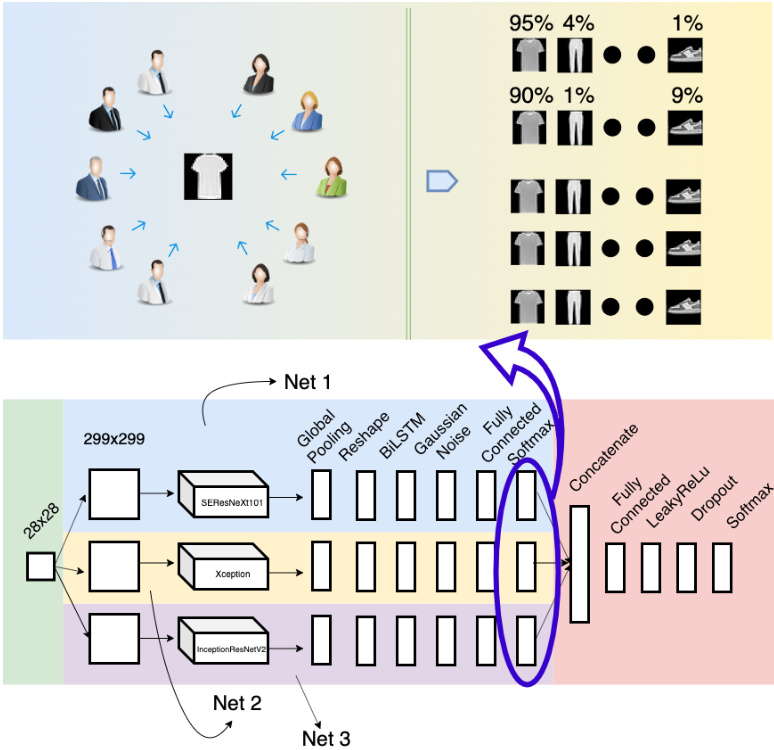
Fig. 1. End-to-end Ensembles of Multiple Models: Concept and Design. The upper part of this image illustrates our key idea, in which several actors make predictions for a sample and output the probability of the sample belonging to each category. The lower part presents a ConvNet design in which three distinct and recent models are aggregated and trained using advanced neural networks. This design also illustrates our proposal of integrating an RNN into an image recognition model. (Best viewed in color)
图 1: 端到端多模型集成:概念与设计。图像上半部分展示了我们的核心思想,其中多个执行者 (actor) 对样本进行预测并输出该样本属于每个类别的概率。下半部分展示了一个卷积网络 (ConvNet) 设计,该设计通过先进神经网络聚合并训练了三个不同的最新模型。此设计也展示了我们将循环神经网络 (RNN) 集成到图像识别模型中的提案。(建议彩色查看)
Ensemble learning is a key aspect of this design. An ensemble refers to an aggregation of weaker models (base learners) combined to construct a model that performs more efficiently (a strong learner) [39]. The ensembling technique is more prevalent in machine learning than in deep learning, especially in the image recognition field, because convolution requires considerable computational power. Most of the recent related studies focus on a simple averaging or voting mechanism [40], [41], [42], [43], [44], and few have investigated integrating trainable neural networks [45], [46]. Our research differs from prior studies, because we study the design on a much larger scale using a larger number of up-to-date ConvNets.
集成学习是该设计的关键部分。集成 (ensemble) 指通过组合多个较弱模型 (基学习器) 来构建性能更优模型 (强学习器) 的方法 [39]。与深度学习相比,集成技术在机器学习领域更为常见,尤其在图像识别领域,因为卷积运算需要大量计算资源。近期相关研究多集中于简单平均或投票机制 [40] [41] [42] [43] [44],而较少探索可训练神经网络的集成方法 [45] [46]。本研究区别于先前工作之处在于,我们采用了更多最新卷积网络 (ConvNet) 进行大规模设计研究。
Suppose that our ConvNet design has $n$ fine-tuned models or class if i ers and that the dataset contains $c$ classes. The output of each classifier can be represented as a distribution vector:
假设我们的卷积网络 (ConvNet) 设计包含 $n$ 个微调模型或分类器,且数据集中有 $c$ 个类别。每个分类器的输出可表示为分布向量:
$$
\Delta_{j}=[\delta_{1j}\quad\delta_{2j}\quad\ldots\quad\delta_{c j}],
$$
$$
\Delta_{j}=[\delta_{1j}\quad\delta_{2j}\quad\ldots\quad\delta_{c j}],
$$
where
其中
$$
\begin{array}{c}{1\leq j\leq n,}\ {0\leq\delta_{i j}\leq1\quad\forall1\leq i\leq c,}\ {\displaystyle\sum_{i=1}^{c}\delta_{i j}=1.}\end{array}
$$
$$
\begin{array}{c}{1\leq j\leq n,}\ {0\leq\delta_{i j}\leq1\quad\forall1\leq i\leq c,}\ {\displaystyle\sum_{i=1}^{c}\delta_{i j}=1.}\end{array}
$$
After concatenating the outputs of the $n$ class if i ers, the distribution vector becomes
在拼接 $n$ 个分类器的输出后,分布向量变为
$$
\Delta=[\Delta_{1}\quad\Delta_{2}\quad...\quad\Delta_{n}].
$$
$$
\Delta=[\Delta_{1}\quad\Delta_{2}\quad...\quad\Delta_{n}].
$$
For formulaic convenience, we assume that the neural network has only one layer and that the number of neurons is equal to the number of classes. As usual, the networks’ weights, $\Theta_{\cdot}$ , are initialized randomly. The distribution vector is computed as follows:
为便于公式表达,我们假设神经网络仅有一层且神经元数量等于类别数。与常规做法相同,网络权重 $\Theta_{\cdot}$ 采用随机初始化。分布向量计算方式如下:
$$
\Delta^{'}=\Theta\cdot\Delta=[\delta_{1}^{'}\quad\delta_{2}^{'}\quad...\quad\delta_{c}^{'}],
$$
$$
\Delta^{'}=\Theta\cdot\Delta=[\delta_{1}^{'}\quad\delta_{2}^{'}\quad...\quad\delta_{c}^{'}],
$$
where
其中
$$
\begin{array}{c}{{1\leq j\leq c,}}\ {{\delta_{j}^{'}=\displaystyle\sum_{i=1}^{n c}\delta_{i}w_{i j}.}}\end{array}
$$
$$
\begin{array}{c}{{1\leq j\leq c,}}\ {{\delta_{j}^{'}=\displaystyle\sum_{i=1}^{n c}\delta_{i}w_{i j}.}}\end{array}
$$
Finally, after the softmax activation, the output is
最后,经过 softmax 激活后,输出为
$$
\eta_{j}^{'}=\frac{e^{\delta_{j}^{'}}}{\displaystyle\sum_{i=1}^{c}e^{\delta_{j}^{'}}}.
$$
$$
\eta_{j}^{'}=\frac{e^{\delta_{j}^{'}}}{\displaystyle\sum_{i=1}^{c}e^{\delta_{j}^{'}}}.
$$
4 EXPERIMENTS
4 实验
In this section, we will present the experiments used to evaluate our initial design (without an RNN) and then analyze the performance when RNNs are integrated. We also describe our end-to-end ensemble multiple models, the developed training strategy, and the extension of the softmax layer. These experiments were performed on the i Naturalist’19 [47] and iCassava’19 Challenges [48], and on the Cifar-10 [49] and Fashion-MNIST [50] datasets. We also extend our experiments on Cifar-100 [49], SVHN [51] and Surrey [52].
在本节中,我们将展示用于评估初始设计(不含RNN)的实验,并分析集成RNN后的性能表现。同时阐述端到端集成多模型方案、开发的训练策略以及softmax层的扩展设计。实验在iNaturalist'19 [47]、iCassava'19挑战赛[48]、Cifar-10 [49]和Fashion-MNIST [50]数据集上进行,并扩展至Cifar-100 [49]、SVHN [51]和Surrey [52]数据集。
4.1 Experiment 1
4.1 实验 1
Deep learning [53] and convolutional neural networks (ConvNets) have achieved notable successes in the image recognition field. From the early LeNet model [54], first proposed several decades ago, to the recent AlexNet [55], Inception [2], [3], [56], ResNet [4], SENet [7] and EfficientNet [8] models, these ConvNets have leveraged automated classification to exceed human performance in several applications. This efficiency is due to the high availability of powerful computer hardware, specifically GPUs and big data.
深度学习 [53] 和卷积神经网络 (ConvNets) 在图像识别领域取得了显著成就。从几十年前首次提出的早期 LeNet 模型 [54],到近期的 AlexNet [55]、Inception [2][3][56]、ResNet [4]、SENet [7] 和 EfficientNet [8] 模型,这些卷积神经网络通过自动分类在多个应用中超越了人类表现。这种高效性得益于强大计算机硬件(特别是 GPU)和大数据的高度可用性。
In this subsection, we examine the significance of our design, which utilizes several ConvNets constructed based on leading architectures such as Inception V 3, ResNet50, Inception-ResNetV2, Xception, Mobile Ne tV 1 and SEResNeXt101. We adopt Inception V 3 as a baseline model since the popularity of ConvNets among deep learning researchers means they can often be used as standard testbeds. In addition, Inception V 3 is known for employing sliding kernels, e.g., $1{\times}1,3{\times}3$ or $5\times5,$ in parallel, which essentially reduces the computation and increases the accuracy. We also use the simplest version of residual networks, i.e., . ResNet50 (ResNet has several versions, including ResNet50, ResNet101 and ResNet152, named according to the number of depth layers), which introduces short circuits through each network layer that greatly reduce the training time. In addition, we explore other ConvNets to facilitate the comparisons and evaluations.
在本小节中,我们将探讨设计方案的重要性。该方案采用了基于主流架构构建的多个卷积神经网络 (ConvNet),包括 Inception V 3、ResNet50、Inception-ResNetV2、Xception、MobileNetV1 和 SEResNeXt101。由于卷积神经网络在深度学习研究者中的普及性使其常被用作标准测试平台,我们选择 Inception V 3 作为基线模型。此外,Inception V 3 以并行使用滑动核(如 $1{\times}1,3{\times}3$ 或 $5\times5$)而闻名,这有效降低了计算量并提升了准确率。我们还采用了残差网络的最简版本 ResNet50(ResNet 系列包含 ResNet50、ResNet101 和 ResNet152 等版本,其命名依据网络深度层数),该架构通过每层引入短路连接大幅缩短了训练时间。同时,我们还测试了其他卷积神经网络以进行对比评估。
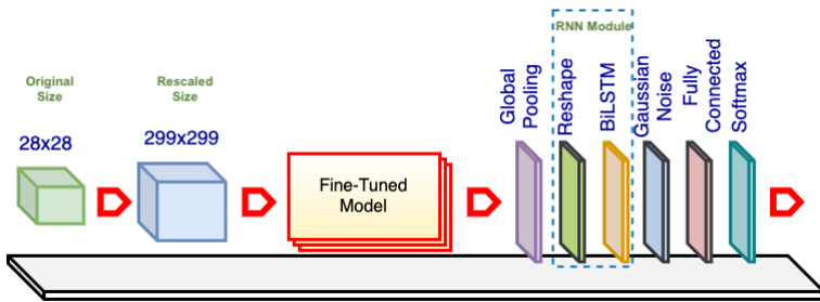
Fig. 2. Single E2E-3M Model. The fine-tuned model is a pretrained ConvNet (e.g., Inception V 3) with the top layers excluded and the weights retrained. The base model comes preloaded with ImageNet weights. The original images are rescaled as needed to match the required input size of the fine-tuned model or for image resolution analysis. The global pooling layer reduces the networks’ size, and the reshaping layer converts the data to a standard input form for the RNN layer. The Gaussian noise layer improves the variation among samples to prevent over fitting. The fully connected layer aims to improve classification. The softmax layer is another fully connected layer that has the same number of neurons as the number of dataset categories, and it utilizes softmax activation.
图 2: 单端到端三模态 (E2E-3M) 模型。微调后的模型是一个预训练的卷积网络 (如 Inception V3),去除了顶层并重新训练权重。基础模型预载了 ImageNet 权重。原始图像会根据需要调整尺寸,以匹配微调模型所需的输入尺寸或用于图像分辨率分析。全局池化层减小网络规模,重塑层将数据转换为 RNN 层的标准输入形式。高斯噪声层通过增加样本间差异性来防止过拟合。全连接层用于提升分类性能。softmax 层是另一个全连接层,其神经元数量与数据集类别数相同,并采用 softmax 激活函数。
Our initial design is depicted in Figure 2. The core of this process implements one of the above mentioned ConvNet models. While the architectures of these ConvNets differ, usually their top layers function as class if i ers and can be replaced to adapt the models to different datasets. For example, Xception and ResNet50 use a global pooling and a fully connected layer as the top layers, while VGG19 [57] uses a flatten layer and two fully connected layers (the original article used max pooling, but for some reason the Keras implementation uses a flatten layer).
我们的初始设计如图 2 所示。该流程的核心实现了上述 ConvNet 模型之一。虽然这些 ConvNet 的架构各不相同,但通常它们的顶层作为分类器 (class if i ers) 使用,可以通过替换来使模型适应不同的数据集。例如,Xception 和 ResNet50 使用全局池化 (global pooling) 和全连接层 (fully connected layer) 作为顶层,而 VGG19 [57] 使用展平层 (flatten layer) 和两个全连接层 (原始论文使用了最大池化 (max pooling),但出于某些原因,Keras 实现使用了展平层)。
Our design adds global pooling to decrease the output size of the networks (this is in line with most ConvNets but contrasts with VGGs, in which flatten layers are utilized extensively). Notably, we also insert an RNN module to evaluate of our proposed approach. The module comprises a reshape layer and an RNN layer as described in subsection 3.1. Moreover, we add a Gaussian noise layer to increase sample variation and prevent over fitting. In the fully connected layer, the number of neurons varies , (e.g., 256, 512, 1024 or 2048); the actual value is based on the specific experiment. The softmax layer uses the same number of outputs as the number of i Naturalist’19 categories.
我们的设计采用全局池化来减小网络输出尺寸(这与大多数卷积网络一致,但与广泛使用扁平层的VGG网络形成对比)。值得注意的是,我们还插入了一个RNN模块来评估所提出的方法。如第3.1小节所述,该模块包含一个重塑层和一个RNN层。此外,我们添加了高斯噪声层以增加样本多样性并防止过拟合。在全连接层中,神经元数量可变(例如256、512、1024或2048),具体数值根据实验而定。softmax层的输出数量与iNaturalist'19数据集的类别数相同。
All the networks’ layers from the ConvNets are unfrozen; we reuse only the models’ architectures and pretrained weights (these ConvNets are pretrained on the ImageNet dataset [58], [59]). Reusing the trained weights offers several advantages because retraining from scratch takes days, weeks or even months on a large dataset such as ImageNet. Typically, transfer learning can be used for most applications based on the concept that the early layers act like edge and curve filters; once trained, ConvNets can be reused on other, similar datasets [57]. However, when the target dataset differs substantially from the pretrained dataset, retraining or fine-tuning can increase the accuracy. To distinguish these ConvNets from the original ones, we refer to each model as a fine-tuned model.
所有卷积网络(ConvNets)的层都被解冻;我们仅复用模型架构与预训练权重(这些卷积网络在ImageNet数据集[58][59]上进行了预训练)。复用训练好的权重具有多重优势,因为在ImageNet等大型数据集上从头开始训练需要数日、数周甚至数月时间。通常,基于早期层充当边缘和曲线滤波器的概念,迁移学习可适用于大多数应用场景;一旦完成训练,卷积网络便可复用于其他相似数据集[57]。然而当目标数据集与预训练数据集差异显著时,重新训练或微调能提升准确率。为区分这些卷积网络与原始模型,我们将每个模型称为微调模型。
We conduct our experiments on the i Naturalist’19 dataset, which was originally compiled for the i Naturalist Challenge, conducted at the 6th Fine-grained Visual Categorization (FGVC6) workshop at CVPR 2019. In the computer vision area, FGVC has been a focus of researchers since approximately 2011 [60], [61], [62], although research on similar topics appeared long before [63], [64]. FGVC or subordinate categorization aims to classify visual objects at a more subtle level of detail than basic level categories [65], for example, bird species rather than just birds [60], dog types [62], car brands [66], and aircraft models [67]. The i Naturalist dataset was created in line with the development of FGVC [47], and the dataset is comparable with ImageNet regarding size and category variation. The specific dataset used in this research (i Naturalist’19) focuses on more similar categories than previous versions and is composed of 1,010 species collected from approximately two hundred thousand real plants and animals. Figure 3 shows some random images from this dataset and indicates the species shown as well as their respective classes and subcategories.
我们在iNaturalist'19数据集上进行了实验,该数据集最初是为2019年CVPR会议第六届细粒度视觉分类(FGVC6)研讨会举办的iNaturalist挑战赛而构建的。在计算机视觉领域,FGVC自2011年左右[60][61][62]就成为研究热点,但类似主题的研究早在[63][64]就已出现。FGVC或下属分类旨在比基础类别[65]更精细的层次上对视觉对象进行分类,例如区分鸟类物种而非仅识别鸟类[60]、犬种[62]、汽车品牌[66]以及飞机型号[67]。iNaturalist数据集是顺应FGVC发展而创建的[47],其规模和类别多样性与ImageNet相当。本研究使用的特定数据集(iNaturalist'19)聚焦于比以往版本更具相似性的类别,包含从约20万真实动植物中收集的1,010个物种。图3展示了该数据集中的随机图像样本,并标注了所示物种及其对应的纲目和亚类。
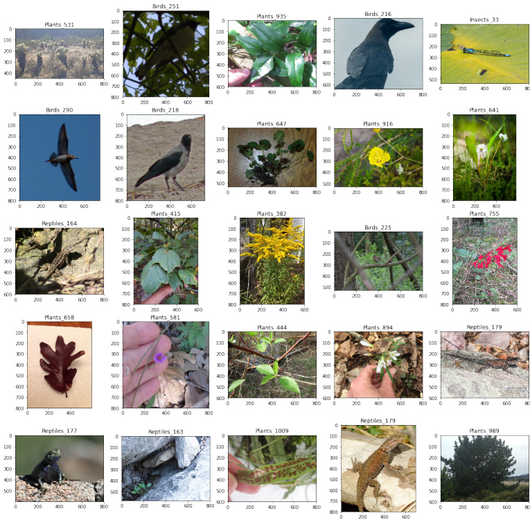
Fig. 3. Random Samples from i Naturalist’19 dataset. Each image is labeled with the species name and its subcategory
图 3: iNaturalist'19 数据集中的随机样本。每张图像都标有物种名称及其子类别
The dataset is randomly split into training and test sets at a ratio of $80:20$ . In addition, the images are resized to appropriate resolutions, e.g., for the Inception V 3 standard, the rescaled images have a size of $299\times299$ . The resolution is also increased to $401\times401$ or even $421\times421$ . In the Gaussian noise layer, we set the amount of noise to 0.1, and in the fully connected layer, we chose $1,024$ neurons based on experience, because it is impractical to evaluate all the layers with every setting.
数据集按 $80:20$ 的比例随机划分为训练集和测试集。此外,图像被调整为适当的分辨率,例如对于 Inception V3 标准,调整后的图像尺寸为 $299\times299$。分辨率也可提升至 $401\times401$ 甚至 $421\times421$。在高斯噪声层中,我们将噪声量设为 0.1;在全连接层中,基于经验选择了 $1,024$ 个神经元,因为对所有层进行每种设置评估是不现实的。
We configured a Jupyter Notebook server running on a Linux operating system (OS) using 4 GPUs (GeForce® GTX 1080 Ti) each with 12 GB of RAM. For coding, we used Keras with a TensorFlow backend [68] as our platform. Keras is written in the Python programming language and has been developed as an independent wrapper that runs on top of several backend platforms, including TensorFlow. The project was recently acquired by Google Inc. and has become a part of TensorFlow.
我们在一台运行Linux操作系统的服务器上配置了Jupyter Notebook环境,使用4块显存为12GB的GeForce® GTX 1080 Ti GPU。代码实现采用基于TensorFlow后端[68]的Keras框架。该框架使用Python语言编写,最初是作为可运行于TensorFlow等后端平台的独立封装层开发,现已被Google公司收购并整合为TensorFlow的组成部分。
Figure 4 shows the results of this experiment in which the top-1 accuracy is plotted against the floating-point operations per second (FLOPS). The size of each model or the total number of parameters is also displayed. The top-1 accuracy was obtained by submitting predictions to the challenge website, obtaining the top-1 error level from the private leader board and subtracting the result from 1. During a tournament, the public leader board is computed based on $51%$ of the official test data. After the tournament, the private leader board contains a summary of all the data.
图 4: 展示了该实验结果,其中纵轴为top-1准确率,横轴为每秒浮点运算次数(FLOPS)。各模型规模(即参数量)亦标注于图中。top-1准确率通过向挑战网站提交预测结果获得,具体计算方式为:从私有排行榜获取top-1错误率后用1减去该数值。竞赛期间公开排行榜基于51%的官方测试数据生成,赛事结束后私有排行榜将汇总全部测试数据。
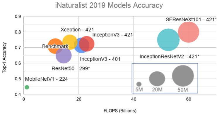
Fig. 4. i Naturalist’19 Model Accuracy. Here, “Benchmark“ denotes the Inception V 3 result using the default input setting (an image resolution of $299\times299$ ). The sizes of the input images for the other models are indicated along with their respective names. For example, Xception-421 indicates that the input images for that model have been rescaled to $421\times421$ .
图 4: iNaturalist'19 模型准确率。其中 "Benchmark" 表示采用默认输入设置 (图像分辨率 $299\times299$) 的 Inception V3 结果。其他模型的输入图像尺寸标注在各自名称旁,例如 Xception-421 表示该模型的输入图像被调整为 $421\times421$。
As expected, a higher image resolution yields greater accuracy but also uses more computing power for the same model (Inception V 3). As a side note, our benchmark achieved an accuracy of 0.7097, which is a marginal gap from the benchmark model on the Challenge website (0.7139). Because we have no knowledge of the organizers’ ConvNet designs, settings and working environments, we cannot delve further into the reasons for this difference. Later, we increased the image resolutions from $299\times299$ to $401\times401$ and $421\times421$ and switched the fine-tuned models. Using Xception-421, our model obtained an accuracy of approximately 0.7347.
正如预期,更高的图像分辨率在相同模型(Inception V 3)下能带来更高准确率,但也会消耗更多算力。值得一提的是,我们的基准测试准确率为0.7097,与挑战赛官网基准模型(0.7139)存在微小差距。由于不了解组织者采用的卷积网络设计、参数设置及运行环境,我们无法深入探究差异原因。后续我们将图像分辨率从$299\times299$提升至$401\times401$和$421\times421$,并切换微调模型。使用Xception-421时,模型准确率达到了约0.7347。
Because our server is shared, training takes approximately one week each time. This is the reason why we could increase the image size to only $421\times421$ . In addition, we did not obtain the results for SERe s NeXt 101-421, InceptionResNetV2-421 and ResNet50-299in this experiment, but projected their approximated accuracies; we will use these models in later experiments. Additionally, because adding an RNN module would substantially increase the training time, the RNN module is not analyzed on the i Naturalist’19
由于我们的服务器是共享的,每次训练大约需要一周时间。这就是为什么我们只能将图像尺寸增加到 $421\times421$。此外,在本实验中我们未获得SEResNeXt 101-421、InceptionResNetV2-421和ResNet50-299的结果,但预估了它们的近似准确率;我们将在后续实验中使用这些模型。另外,由于添加RNN模块会显著增加训练时间,因此未在iNaturalist'19数据集上分析RNN模块。
dataset.
数据集
4.2 Experiment 2
4.2 实验 2
As mentioned in the previous section, most of the research regarding RNNs has focused on sequential data or time series. Despite the little attention paid to using RNNs with images, the main goal is to generate sequences of pixels rather than direct image recognition. Our approach differs significantly from typical image recognition models, in which all the image pixels are presented simultaneously rather than in several time steps.
如前一节所述,大多数关于RNN的研究都集中在序列数据或时间序列上。尽管很少有人关注将RNN用于图像,但其主要目标是生成像素序列而非直接的图像识别。我们的方法与典型的图像识别模型有很大不同,后者所有图像像素是同时呈现的,而非分多个时间步呈现。
We systematically evaluated the proposed design that utilizes distinct recurrent neural networks. These models include a typical RNN, an advanced GRU and a bidirectional RNN–BiLSTM—and we compared them against a standard (STD) model without an RNN module. In addition, we selected representative fine-tuned models, namely, Inception V 3, Xception, ResNet50, Inception-ResNetV2, MobileNetV1, VGG19 and SERe s NeXt 101, for comparison and analysis.
我们系统评估了所提出的采用不同循环神经网络的设计方案。这些模型包括典型RNN、先进的GRU以及双向RNN——BiLSTM,并将其与不含RNN模块的标准(STD)模型进行对比。此外,我们选取了具有代表性的微调模型进行比较分析,包括Inception V3、Xception、ResNet50、Inception-ResNetV2、MobileNetV1、VGG19以及SEResNeXt 101。
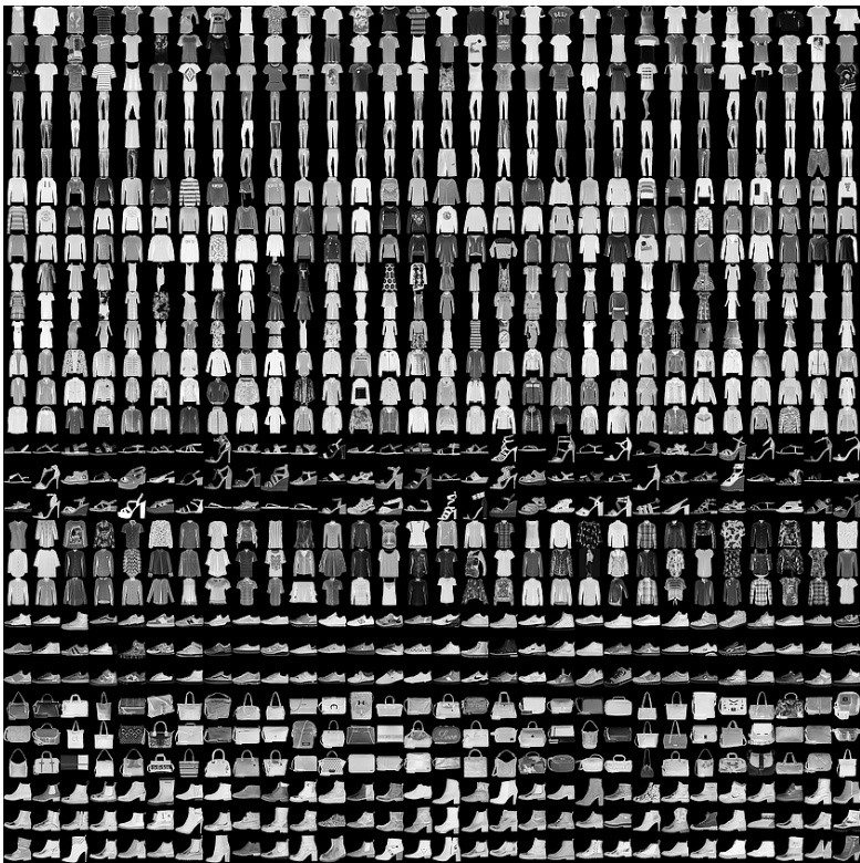
Fig. 5. Some Samples from the Fashion-MNIST dataset
图 5: Fashion-MNIST 数据集中的部分样本
In this experiment, we employ the Fashion-MNIST dataset, which was recently created by Zalando SE and intended to serve as a direct replacement for the MNIST dataset as a machine learning benchmark because some models have achieved an almost perfect result of $100%$ accuracy on MNIST. The Fashion-MNIST dataset contains the same amount of data as MNIST–50, 000 training and 10, 000 testing samples–and includes 10 categories. Figure 5 visualizes how this dataset looks; each sample is a $28\times28$ grayscale image.
在本实验中,我们采用了由Zalando SE最新创建的Fashion-MNIST数据集。该数据集旨在作为MNIST数据集的直接替代品,成为机器学习的新基准,因为部分模型在MNIST上已能达到接近完美的$100%$准确率。Fashion-MNIST与MNIST数据量相同——包含50,000个训练样本和10,000个测试样本——并涵盖10个类别。图5展示了该数据集的可视化效果:每个样本均为$28\times28$的灰度图像。
Our initial design (as discussed previously) is reused with a highlighted note that the RNN module has been incorporated. The number of units for each RNN is set to 2,048 (in the BiLSTM, the number of units is 1,024); the time step number is simply one, which shows the entire image each time. In addition, because the image size in the FashionMNIST dataset is smaller than the desired resolutions (e.g., $244\times244$ or $299\times299$ for Mobile Ne tV 1 and Inception V 3), all the images are upsampled.
我们沿用了初始设计 (如前所述),并特别注明已整合RNN模块。每个RNN单元数设置为2,048 (BiLSTM中单元数为1,024);时间步数仅为1,表示每次呈现完整图像。此外,由于FashionMNIST数据集的图像尺寸小于目标分辨率 (例如MobileNetV1和InceptionV3所需的$244\times244$或$299\times299$),所有图像都进行了上采样处理。
TABLE 1 Accuracy comparison of models using distinct recurrent neural networks built on Inception V 3 and Mobile Ne tV 1
表 1: 基于 Inception V3 和 MobileNetV1 构建的不同循环神经网络模型准确率对比
| 微调模型 | STD | RNN | GRU | BiLSTM |
|---|---|---|---|---|
| InceptionV3 | 0.9434 | 0.9453 | 0.9430 | 0.9445 |
| MobileNetV1 | 0.9404 | 0.9438 | 0.9439 | 0.9410 |
We performed these experiments on Google Colab1, even though our server runs faster. The main reason is that Jupyter Notebook occupies all the GPUs for the first login section. In other words, only one program executes with full capability. In contrast, Colab can run multiple environments in parallel. A secondary reason is that the virtual environment allows rapid development (i.e., it supports the installation of additional libraries and can run programs instantly). All the experiments are set to run for 12 hours; some take less time before over fitting, but others take more than the maximum time allotted. We repeated each experiment 3 times. Moreover, in this study, we often submit the results to challenge websites and record only the highest accuracy rather than employing other metrics. The accuracy metric is defined as follows:
我们在Google Colab1上进行了这些实验,尽管我们的服务器运行速度更快。主要原因是Jupyter Notebook在首次登录时会占用所有GPU资源,换句话说,只有单个程序能全性能执行。相比之下,Colab可以并行运行多个环境。次要原因是虚拟环境支持快速开发(即支持安装额外库并能即时运行程序)。所有实验均设置为运行12小时:部分实验在过拟合前耗时较短,但其他实验会超出最大分配时长。每组实验重复3次。此外,本研究中我们常将结果提交至挑战网站,仅记录最高准确率而非采用其他指标。准确率指标定义如下:
$$
A c c u r a c y={\frac{\mathrm{Number of correct predictions}}{\mathrm{Total numbers of predictions~made}}}.
$$
$$
A c c u r a c y={\frac{\mathrm{Number of correct predictions}}{\mathrm{Total numbers of predictions~made}}}.
$$
Table 1 shows comparisons of the various models using different RNN modules built on Inception V 3 and MobileNetV1. The former is often chosen as a baseline model, whereas the latter is the lightest model used here in terms of parameters and computation. The results in Figure 6 show that the models with the additional RNN modules achieve substantially higher accuracy than do the STD models.
表 1 展示了基于 Inception V3 和 MobileNetV1 构建的不同 RNN 模块的模型对比。前者常被选作基线模型,而后者是本文所用参数量和计算量最轻的模型。图 6 结果显示,增加 RNN 模块的模型比 STD 模型取得了显著更高的准确率。
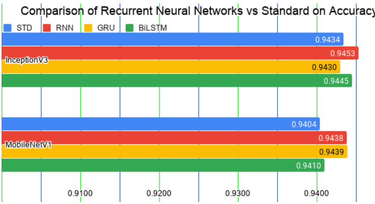
Fig. 6. Accuracy comparison of models integrated with recurrent neural networks vs. the standard model (STD). The integrated models significantly outperform the STD models.
图 6: 集成循环神经网络 (RNN) 的模型与标准模型 (STD) 的准确率对比。集成模型显著优于标准模型。
- https://colab.research.google.com/, which began as an internal project built based on Jupyter Notebook but was opened for public use in 2018. At the time of this writing, the virtual environment supports only a single 12 GB NVIDIA Tesla K80 GPU.
- https://colab.research.google.com/,最初是基于Jupyter Notebook构建的内部项目,于2018年开放公众使用。截至本文撰写时,该虚拟环境仅支持单个12 GB NVIDIA Tesla K80 GPU。
TABLE 2 Comparison of BiLSTM and STD on different fine-tuned models, including Inception V 3, Xception, ResNet50, Inception-ResNetV2, Mobile Ne tV 1, VGG19 and SERe s NeXt 101.
表 2: BiLSTM 和 STD 在不同微调模型上的对比,包括 Inception V3、Xception、ResNet50、Inception-ResNetV2、MobileNetV1、VGG19 和 SEResNeXt 101。
| Fine-tunedModels | ||||
|---|---|---|---|---|
| Inception V3 | Xception | ResNet 50 | InceptionResNet V2 | |
| STD | 0.9434 | 0.9374 | 0.9375 | 0.9364 |
| BiLSTM | 0.9445 | 0.9383 | 0.9377 | 0.9360 |
| MobileNet V1 | VGG19 | SEResNeXt 101 | ||
| STD | 0.9404 | 0.9075 | N/A | |
| BiLSTM | 0.9410 | N/A | N/A |
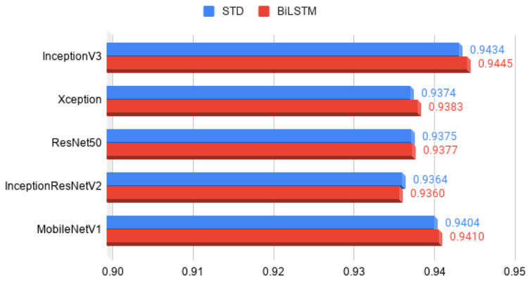
Fig. 7. Comparison of the accuracy of BiLSTM and STD models using Inception V 3, Xception, ResNet50, Inception-ResNetV2 and MobileNetV1. The BiLSTM models substantially outperform the STD models in several instances.
图 7: 使用 Inception V3、Xception、ResNet50、Inception-ResNetV2 和 MobileNetV1 的 BiLSTM 与 STD 模型准确率对比。BiLSTM 模型在多数情况下显著优于 STD 模型。
We also extended this experiment to include more models, including Xception, ResNet50, Inception-ResNetV2, VGG19 and SERe s NeXt 101. Table 2 shows the comparisons of models integrated with the BiLSTM module versus the standard models. Most of the models integrated with BiLSTMs significantly outperform the STDs, except for Inception-ResNetV2. Please note that training the VGG19 model required excessive training time; the model did not reach the same accuracy level as the other models even after 12 hours of training. Similarly, we were unable to obtain results for the VGG19-BiLSTM or SERe s NeXt 101 models. Therefore, Figure 7 shows only the results for Inception V 3, Xception, ResNet50, Inception-ResNetV2 and Mobile Ne tV 1.
我们还扩展了实验范围,纳入了更多模型,包括Xception、ResNet50、Inception-ResNetV2、VGG19和SEResNeXt 101。表2展示了集成BiLSTM模块的模型与标准模型的对比结果。除Inception-ResNetV2外,大多数集成BiLSTM的模型性能显著优于标准模型。需注意,VGG19模型的训练耗时过长,即使经过12小时训练仍未达到其他模型的精度水平。同样,我们未能获得VGG19-BiLSTM和SEResNeXt 101模型的实验结果。因此,图7仅展示了Inception V3、Xception、ResNet50、Inception-ResNetV2和MobileNetV1的结果。
4.3 Experiment 3
4.3 实验3
Often, when training a model, we randomly split a dataset into training and testing sets with a desired ratio. Then, we repeat our evaluation several times, and finally, obtain the results from one of the measurement methods, e.g., accuracy mean and standard deviation. However, in competitions such as those on Kaggle, a test set is completely separated from a training set. If we naively divide the training set into a training set and a validation set, we face a dilemma in which all the samples of the original training set cannot be used for training because a portion of the dataset is always needed for validation. To solve this problem, we apply $\mathbf{k}\cdot\mathbf{\partial}$ - fold validation to the training set by dividing the dataset into $\mathbf{k}$ subsets, of which one is reserved for validation. We expand this process and make predictions on the official test set. This method allows our models (one model for each set) to learn from all the images in the official training set.
在训练模型时,我们通常会将数据集按所需比例随机划分为训练集和测试集。随后进行多次评估,最终通过某种测量方法(如准确率均值和标准差)获得结果。然而,在Kaggle等竞赛中,测试集与训练集是完全分离的。若简单地将训练集划分为训练集和验证集,就会面临原始训练集无法全部用于训练的困境——因为总需要保留部分数据用于验证。为解决这个问题,我们对训练集采用$\mathbf{k}\cdot\mathbf{\partial}$折交叉验证:将数据集分成$\mathbf{k}$个子集,其中留一个子集作为验证集。通过扩展这一流程并对官方测试集进行预测,我们的模型(每个子集对应一个模型)就能从官方训练集的所有图像中学习。
We also attempted to increase model robustness via data augmentation techniques. The goal of such techniques is to transform an original training dataset into an expanded dataset whose true labels are known [69], [70], [71]. Importantly, this teaches the model to be invariant to and un influenced by input variations [72]. For example, flipping an image of a car horizontally does not change its corresponding category. We applied the augmentation approach from [55] on the test set. In this approach a sample is cropped multiple times and the model makes predictions for each instance. The procedure has recently become standard practice in image recognition tasks and is referred to as “test time augmentation.“ In this study, we cropped the images at random locations instead of at only the four corners and the center. In addition, we utilized the most prevalent augmentation techniques for geometric and texture transformations, such as rotation, width/height shifts, shear and zoom, horizontal and vertical flips and channel shift.
我们还尝试通过数据增强技术提高模型的鲁棒性。这类技术的目标是将原始训练数据集转换为已知真实标签的扩展数据集 [69], [70], [71]。关键在于,这能教会模型对输入变化保持不变性且不受其影响 [72]。例如,将汽车图片水平翻转不会改变其对应类别。我们在测试集上应用了 [55] 提出的增强方法:对样本进行多次裁剪,模型对每个裁剪实例进行预测。该流程近期已成为图像识别任务的标准实践,称为"测试时增强 (test time augmentation)"。本研究中,我们采用随机位置裁剪而非仅限四角和中心裁剪。此外,我们运用了最普遍的几何与纹理变换增强技术,包括旋转、宽/高偏移、剪切缩放、水平/垂直翻转以及通道偏移。
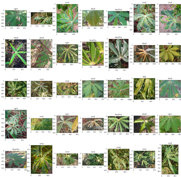
Fig. 8. Random Samples from the iCassava dataset. CMD, CGM, CBB and CBSD denote cassava mosaic disease, cassava green mite disease, cassava bacterial blight, and cassava brown streak disease, respectively.
图 8: iCassava数据集中的随机样本。CMD、CGM、CBB和CBSD分别表示木薯花叶病、木薯绿螨病、木薯细菌性枯萎病和木薯褐条病。
We also applied state-of-the-art ensemble learning because the technique is generally more accurate than is prediction from a single model. We use a simple averaging approach to aggregate all the models (a.k.a AVG-3M). Additionally, it is important to ensure a variety of the finetuned models to increase the classifier diversity because combining multiple redundant class if i ers would be meaningless. We finally chose the SERest NeXt 101, Xception and Inception-ResNetV2 fine-tuned models, as these ConvNets yield higher results than do others. Please note that the RNN module (including the reshape and BiLSTM layers) is excluded.
我们还应用了最先进的集成学习技术,因为该技术通常比单一模型的预测更准确。我们采用简单的平均方法聚合所有模型(即AVG-3M)。此外,确保微调模型的多样性以提升分类器差异性至关重要,因为组合多个冗余分类器毫无意义。最终我们选择了SERest NeXt 101、Xception和Inception-ResNetV2微调模型,这些卷积网络的性能优于其他模型。需注意,RNN模块(包括重塑层和双向LSTM层)被排除在外。
One last crucial technique is our training strategy, which helps to reduce loss and increase accuracy by searching for a better global minimum (more details will be presented in the next section).
最后一项关键技术是我们的训练策略,它通过寻找更好的全局最小值来帮助减少损失并提高准确度 (更多细节将在下一节中介绍)。
We evaluated our approach using the iCassava Challenge dataset, which was also compiled for the FGVC6 workshop at CVPR19. In the iCassava dataset, the leaf images of cassava plants are divided into 4 disease categories: cassava mosaic disease, cassava green mite disease, cassava bacterial blight, and cassava brown streak disease, and 1 category of healthy plants, comprising 9,436 labeled images. The challenge was organized on the Kaggle website 2, ran from the 26th of April to the 2nd of June 2019, and attracted nearly 100 teams from around the world. The proposed models were evaluated on 3,774 official test samples, and the results were submitted to the website. The public leader board is computed from $40%$ of the test data, whereas the private leader board is computed from all the test data. Figure 8 shows some random samples from this dataset.
我们使用iCassava Challenge数据集评估了我们的方法,该数据集也是为CVPR19的FGVC6研讨会所整理。在iCassava数据集中,木薯植物的叶片图像被分为4种病害类别:木薯花叶病、木薯绿螨病、木薯细菌性枯萎病和木薯褐条病,以及1类健康植物,共包含9,436张标注图像。该挑战赛于2019年4月26日至6月2日在Kaggle网站2上举办,吸引了来自全球近100支团队参赛。所提出的模型在3,774个官方测试样本上进行了评估,结果提交至网站。公开排行榜基于40%的测试数据计算,而私有排行榜则基于全部测试数据计算。图8展示了该数据集中的一些随机样本。
The iCassava official training set is split into 5 subsets for k-fold cross validation, in which one subset is reserved for testing and the others are used for training in turn. We performed these experiments on a server using a GeForce® GTX 1080 Ti graphics card with 4 GPUs, each with 12 GB of RAM.
iCassava官方训练集被划分为5个子集用于k折交叉验证,其中1个子集留作测试,其余子集依次用于训练。我们在配备GeForce® GTX 1080 Ti显卡(4块GPU,每块12GB显存)的服务器上进行了这些实验。
When evaluating the test set, we upsampled the images to a higher resolution $(540\times540)$ and then randomly cropped them to the input size $(501\times501\$ ). We varied the numbers of crops among 1, 3, 5, 7 and 9, and finally selected just 3 crops, as this option yielded higher accuracy than did the other cropping choices in most subsets. We collected the results for two methods, one without cropping and the other with 3 crops, and selected the one with the higher accuracy for each set. Then, we averaged the results for all the sets to provide a result for the entire dataset. The overall result achieved an accuracy of 0.928.
在评估测试集时,我们将图像上采样至更高分辨率 $(540\times540)$ ,然后随机裁剪至输入尺寸 $(501\times501)$ 。我们尝试了1、3、5、7和9等不同裁剪数量,最终选择仅3次裁剪,因为在大多数子集中该选项比其他裁剪方案具有更高准确率。我们收集了两种方法的结果(无裁剪方案与3次裁剪方案),并为每个子集选择准确率更高的方案。随后对所有子集结果取平均值,得到整个数据集的最终结果,总体准确率达到0.928。

iCassava 2019 Fine-Grain Visual Challenge: Compare with Our Result Fig. 9. Comparison of our AVG-3M result on the iCassava challenge dataset with those of the top-10 teams
图 9: 在iCassava挑战数据集上我们的AVG-3M结果与前十名团队结果的对比
Furthermore, we applied the AVG-3M design to sets number 3, 4 and 5 and averaged each of these results with all other sets. Table 3 shows the results for this experiment. As the table shows, employing our AVG-3M model for these sets improves the accuracy. The combination of AVG-3M on Set 4 with the remaining sets yields the highest result (0.9368). It is critical to note that even though the public leader board result for all sets with the AVG-3M of Set 3 yields a higher result than that of Set 4, eventually, the latter achieved a better result. Therefore, choosing the submission for the final evaluation is efficient and essential. Figure 9 shows our results in comparison with those of other top-10 teams.
此外,我们将AVG-3M设计应用于第3、4、5组数据,并将每组结果与其他所有组进行平均。表3展示了该实验的结果。如表所示,对这些组采用我们的AVG-3M模型能提升准确率。其中,第4组数据结合AVG-3M与其他组数据取得了最高结果(0.9368)。值得注意的是,虽然第3组AVG-3M在公开排行榜上所有组的结果优于第4组,但最终后者取得了更好的成绩。因此,选择最优提交进行最终评估是高效且关键的。图9展示了我们与其他前十团队的结果对比。
4.4 Experiment 4
4.4 实验4
TABLE 3iCassava Result. The dataset is divided into 5 subsets. Four of the subsets are combined to form a training set and the other subset is used as for validation. Each of these combinations (including training and validation sets) composes a dataset, named Sets 1–5. A “Valid“ label denotes results obtained using valid data, while “Private“ and “Public“ represent results obtained from corresponding categories on the challenge website. Test–0 Crop indicates test results obtained without cropping, whereas Test–3 Crop indicates test results obtained using the 3 cropping methods. The best resultsfor each subset are summarized in the table at the bottom left, including both the private and public results. The table on the bottom right represents the results obtained using AVG-3M for each individual set and when each result is combined with all the others
表 3iCassava 结果。该数据集被划分为 5 个子集,其中 4 个子集组合为训练集,另一个子集用于验证。每种组合(包括训练集和验证集)构成一个数据集,分别命名为 Set 1-5。"Valid"标签表示使用验证数据获得的结果,而"Private"和"Public"分别代表挑战网站上相应类别获得的结果。Test-0 Crop 表示未使用裁剪获得的测试结果,Test-3 Crop 表示使用 3 种裁剪方法获得的测试结果。左下角表格汇总了每个子集的最佳结果(包括 private 和 public 结果)。右下角表格表示使用 AVG-3M 方法对每个单独子集及所有子集组合获得的结果。

Fig. 10. Training Strategy. We start with a moderate learning rate so that training does not become stuck in a local minimum. Then, we reduce the learning rate for the 2nd and 3rd iterations. If the learning rate is too large, the global minimum might be ignored; however, if it is too small, the training time becomes excessive.
图 10: 训练策略。我们从一个适中的学习率开始,以避免训练陷入局部最小值。随后,在第二次和第三次迭代时降低学习率。若学习率过大,可能会忽略全局最小值;但若过小,则会导致训练时间过长。
In this subsection, we address the overall improvement of our model using a learning rate strategy. We apply the Adam optimizer [73], which is an advanced optimizer in the deep learning area. The computations are as follows:
在本小节中,我们通过采用学习率策略来全面提升模型性能。我们使用了深度学习领域先进的优化器Adam [73],其计算过程如下:
$$
\begin{array}{c}{{w_{t}=w_{t-1}-\eta_{t}\cdot\displaystyle\frac{m_{t}}{\left(\sqrt{v_{t}}+\hat{\epsilon}\right)},}}\ {{\eta_{t}=\eta\cdot\displaystyle\frac{\sqrt{1-\beta_{2}^{t}}}{1-\beta_{1}^{t}},}}\ {{m_{t}=\beta_{1}\cdot m_{t-1}+\left(1-\beta_{1}\right)\cdot g_{t},}}\ {{v_{t}=\beta_{2}\cdot v_{t-1}+\left(1-\beta_{2}\right)\cdot g_{t}^{2},}}\end{array}
$$
$$
\begin{array}{c}{{w_{t}=w_{t-1}-\eta_{t}\cdot\displaystyle\frac{m_{t}}{\left(\sqrt{v_{t}}+\hat{\epsilon}\right)},}}\ {{\eta_{t}=\eta\cdot\displaystyle\frac{\sqrt{1-\beta_{2}^{t}}}{1-\beta_{1}^{t}},}}\ {{m_{t}=\beta_{1}\cdot m_{t-1}+\left(1-\beta_{1}\right)\cdot g_{t},}}\ {{v_{t}=\beta_{2}\cdot v_{t-1}+\left(1-\beta_{2}\right)\cdot g_{t}^{2},}}\end{array}
$$
where $w$ and $\eta$ are the weight and the learning rate of the neural networks, respectively; $m,v$ and $g$ are the moving averages and gradient of the current mini-batch; and the betas $(\beta_{1},\beta_{2})$ and epsilon $\epsilon$ are set to 0.9, 0.999 and $10^{-8}$ , respectively.
其中 $w$ 和 $\eta$ 分别是神经网络的权重和学习率;$m,v$ 和 $g$ 是当前小批量的移动平均值和梯度;而 beta 值 $(\beta_{1},\beta_{2})$ 和 epsilon $\epsilon$ 分别设为 0.9、0.999 和 $10^{-8}$。
We used Keras to implement the models; on that platform, the formula for computing the learning rate with decay is
我们使用 Keras 来实现模型;在该平台上,计算带衰减的学习率公式为
$$
\eta=\eta\cdot\frac{1}{1+d e c a y\cdot i t e r a t i o n s}.
$$
$$
\eta=\eta\cdot\frac{1}{1+d e c a y\cdot i t e r a t i o n s}.
$$
Choosing an appropriate learning rate is both essential and critical, because the training time is often dramatically reduced with an appropriate learning rate. However, selecting an appropriate learning rate is difficult. When the step size is too large, the global minimum might be ignored, whereas a too-small step size can result in an excessive training time. In these experiments, we started with a moderate learning rate and trained the model until the accuracy stopped improving. Then, we reduced the learning rate, reloaded the ConvNet weights that achieved the highest accuracy and repeated this process for two more times. Figure 10 illustrates our proposed training procedure.
选择合适的学习率既重要又关键,因为适当的学习率通常能大幅缩短训练时间。然而,选取合适的学习率十分困难:步长过大会错过全局最小值,步长过小则会导致训练时间过长。在这些实验中,我们首先采用中等学习率训练模型直至准确率停止提升,随后降低学习率并重新加载达到最高准确率的卷积神经网络权重,此过程重复执行两次。图10展示了我们提出的训练流程。

Fig. 11. Model Accuracy on the Fashion-MNIST dataset Using Our Training Strategy. The models are trained with a learning rate starting at $1e^{-4}$ for 40 epochs. The RNN modules (STD, RNN, LSTM and GRU) are compared. The best module is selected for each model, e.g., the BiLSTM for Xception. The models are reloaded with the highest check points and trained two more times for 15 epochs each at learning rates of $1e^{-5}$ and $1e^{-6}$ , respectively.
图 11: 采用我们训练策略在 Fashion-MNIST 数据集上的模型准确率。模型以 $1e^{-4}$ 的学习率训练 40 个周期,对比了 STD、RNN、LSTM 和 GRU 等循环神经网络模块。每个模型选用最佳模块(例如 Xception 采用 BiLSTM),加载最高检查点后分别以 $1e^{-5}$ 和 $1e^{-6}$ 学习率各追加训练 15 个周期。
We evaluated these experiments on the Cifar-10 and Fashion-MNIST datasets. Initially, the learning rate was set to $1e^{-4}$ and then sequentially changed to $1e^{-5}$ and $1e^{-6}$ . The decay was derived by dividing the learning rate by the number of epochs.
我们在Cifar-10和Fashion-MNIST数据集上评估了这些实验。初始学习率设置为$1e^{-4}$,随后依次调整为$1e^{-5}$和$1e^{-6}$。衰减值通过将学习率除以训练周期数得出。
Figure 11 shows the performances of the top 3 models on Fashion-MNIST using SERe s NeXt 101 STD, Xception LSTM and Inception-ResNetV2 STD and the figure excludes the results of other ConvNets discussed in the previous sections. The three RNN variations were also analyzed against the STD models, and only the model with the highest accuracy is shown in the figure. The accuracies are effectively increased after the transition. SERe s NeXt 101 achieved a result of 0.9541 under the STD setting.
图 11 展示了使用 SERe s NeXt 101 STD、Xception LSTM 和 Inception-ResNetV2 STD 的 top 3 模型在 Fashion-MNIST 上的性能表现,该图排除了前几节讨论的其他卷积网络的结果。我们还针对 STD 模型分析了三种 RNN 变体,图中仅展示了准确率最高的模型。转换后准确率显著提升,SERe s NeXt 101 在 STD 设置下达到了 0.9541 的结果。
This result was further improved to 0.9585 when using the E2E-3M model The design is shown in Figure 1, and the steps are detailed in Algorithm 1. The settings were as follows: the fully connected layer (after the concatenation layer) had 4,096 neurons; the LeakyReLU had a slope of 0.2 and dropout was set at 0.5. Please note that when reloading weights, we sometimes need to convert the weights to Pickle format rather than Keras’ standard HDF5 format because the networks’ weights are too large.
使用E2E-3M模型时,该结果进一步提升至0.9585。设计如图1所示,具体步骤详见算法1。参数设置如下:全连接层(位于拼接层之后)包含4096个神经元;LeakyReLU斜率为0.2,dropout设置为0.5。请注意,重新加载权重时,由于网络权重过大,有时需要将权重转换为Pickle格式而非Keras标准HDF5格式。
We conducted experiments in the same manner on the Cifar-10 dataset. The results are shown in Figure 12. Please note that we also added Efficient Net B 5, as this ConvNet is one of the latest models in the field. Using Efficient Net B 5, we achieved an accuracy of 0.9788 under the STD setting.
我们在Cifar-10数据集上以相同方式进行了实验。结果如图12所示。请注意,我们还添加了Efficient Net B 5,因为该卷积网络(ConvNet)是该领域最新模型之一。使用Efficient Net B 5时,我们在STD设置下达到了0.9788的准确率。
In summary, our learning rate strategy differs from conventional methods, where the learning rates are predefined
总之,我们的学习率策略不同于传统方法中预定义学习率的做法
Algorithm 1 E2E-3M
算法 1 E2E-3M
Input: A training set with c categories $D$ := $(a_{1},b_{1}),(a_{2},b_{2})\bar{.}..(a_{n},b_{n})$
输入:一个包含c个类别的训练集 $D$ := $(a_{1},b_{1}),(a_{2},b_{2})\bar{.}..(a_{n},b_{n})$
Output: Class Predictions
输出:类别预测
$$
M_{i}=(a_{i}^{'},b_{i})
$$
$$
M_{i}=(a_{i}^{'},b_{i})
$$
where:
其中:
$$
\begin{array}{c}{{a_{i}^{'}=[\Delta_{1}(a_{i})\Delta_{2}(a_{i})\Delta_{3}(a_{i})]^{T}}}\ {{\Delta_{j}=[\delta_{1}\delta_{2}...\delta_{c}]}}\end{array}
$$
$$
\begin{array}{c}{{a_{i}^{'}=[\Delta_{1}(a_{i})\Delta_{2}(a_{i})\Delta_{3}(a_{i})]^{T}}}\ {{\Delta_{j}=[\delta_{1}\delta_{2}...\delta_{c}]}}\end{array}
$$
7: end for
7: end for
8: Step 6: Train $\lambda$ neurons in the fully connected neural networks $(M)$
8: 步骤6: 在全连接神经网络 $(M)$ 中训练 $\lambda$ 神经元
$$
\mu_{j}=\sum_{i=0}^{3c-1}\delta_{i}w_{i j},1\leq j\leq\lambda
$$
$$
\mu_{j}=\sum_{i=0}^{3c-1}\delta_{i}w_{i j},1\leq j\leq\lambda
$$
9: Step 7: Apply LeakyReLU activation $({\mathsf{s l o p e}}=k)$
9: 步骤7: 应用LeakyReLU激活函数 $({\mathsf{s l o p e}}=k)$
10: Step 8: Regularize using dropout (rate $=p$ )
10: 步骤 8: 使用 dropout (比率 $=p$) 进行正则化
$$
v_{j}=\gamma\eta_{j}
$$
$$
v_{j}=\gamma\eta_{j}
$$
where $\gamma$ is a gating variable 0-1 that follows a Bernoulli distribution with $P(\gamma=1)=p$ 11: Step 9: Train the Final Fully Connected Neural Networks 12: Step 10: Apply Softmax
其中 $\gamma$ 是遵循伯努利分布的门控变量(0-1),其 $P(\gamma=1)=p$
11: 步骤9: 训练最终的全连接神经网络
12: 步骤10: 应用Softmax

Fig. 12. Model Accuracies on Cifar-10 Using Our Training Strategy. The models are trained with a learning rate starting at $1e^{-4}$ for 40 epochs. Then the RNN modules (including STD, RNN, LSTM and GRU) are compared. The best module is selected for each model, (e.g., STD in the case of Efficient Net B 5). The models are then reloaded with the highest checkpoints and trained twice more for 15 epochs each at learning rates of $1e^{-5}$ and $1e^{-6}$ , respectively.
图 12: 采用我们训练策略在Cifar-10上的模型准确率。模型初始学习率为 $1e^{-4}$ 训练40轮,随后比较RNN模块(包括STD、RNN、LSTM和GRU),为每个模型选择最佳模块(例如Efficient Net B5选用STD)。接着重新加载最高检查点,分别以 $1e^{-5}$ 和 $1e^{-6}$ 学习率各训练15轮。
based on experiments. Applying an adaptive learning rates offers more flexibility to adjust the learning rates automatically during training. Our approach applies the Adam optimizer but in an intuitive way. After training for some epochs with the optimizer, the models begin over fitting. Thus, in our method, we reduce the learning rate and reload the best model, which leverages the accuracy to a higher point.
基于实验。采用自适应学习率能够在训练过程中更灵活地自动调整学习率。我们的方法以一种直观的方式应用了Adam优化器。在使用该优化器训练若干周期后,模型开始出现过拟合现象。因此,在我们的方法中,我们会降低学习率并重新加载最佳模型,从而将准确率提升至更高水平。
4.5 Experiment 5
4.5 实验5
In this subsection, our setup includes a variation of the softmax layer in which only the outputs of the most active neurons are used for prediction. We observe that in multi category prediction, often, only a few or even just one confidence value on a category is large enough to be meaningful, while others are very small, i.e., a confidence level of nearly zero percent. For this reason, we propose eliminating meaningless confidence levels by zeroing them before use in ensembling. We compared this approach (namely, EXTSoftmax) with a typical method where multiple predictions are averaged to obtain a final prediction (AVG-Softmax). The essential steps are illustrated in Algorithm 2.
在本小节中,我们的设置包含了一个softmax层的变体,其中仅使用最活跃神经元的输出来进行预测。我们观察到,在多类别预测中,通常只有少数甚至仅一个类别的置信度值足够大而有意义,而其他值非常小,即置信度接近于零。因此,我们提出在集成前将这些无意义的置信度归零以消除其影响。我们将这种方法(称为EXTSoftmax)与典型的多预测平均法(AVG-Softmax)进行了比较。关键步骤如算法2所示。
The results on Fashion-MNIST are 0.9592 and 0.9591 without improvement using the proposed approach. However, on Cifar-10, the accuracy is higher, ranging from 0.9833 to 0.9836. Tables 4 and 5 show the latest achievements on these datasets. Please note that the Fashion-MNIST results were voluntarily submitted and were not officially verified. However, we analyzed each profile and selected only results that are supported by publications. Importantly, the dataset was changed recently to eliminate duplicates ; our results might have been even higher if the previous version had been used.
在Fashion-MNIST数据集上,使用所提方法后的结果为0.9592和0.9591,未见提升。而在Cifar-10数据集上准确率更高,介于0.9833至0.9836之间。表4和表5展示了这些数据集的最新成果。需注意,Fashion-MNIST的结果为自愿提交且未经官方验证。但我们分析了每个档案,仅筛选有论文支撑的结果。关键的是,该数据集近期经过更新以消除重复项;若使用旧版本,我们的结果可能会更高。
TABLE 5 List of recent achievements on Cifar-10 along with the results of our models. The proposed approach performs comparably to the top models.
表 5: Cifar-10最新成果列表及我们模型的实验结果。所提出的方法与顶级模型表现相当。
| 算法 2Pruning | |
|---|---|
| 输入: Prediction Confidence A 输出: Pruned A | |
| 1: function PRUNE(A) | |
| 2: | N←length(A) |
| 3: | M←length(A[o]) |
| 4: | for i ← 0 to N - 1 do |
| 5: | inderMax←findInderOfMaxValue(A) |
| 6: | for j ← 0 to M - 1 do |
| 7: | ifA[i]≠indexMarthen |
| 8: | A[i] ← 0 |
| 9: | end if |
| 10: | end for |
| 11: | end for |
| 12: | return A |
| 13:end function |
4.6 Experiment 6
4.6 实验6
In this subsection, we extend our experiments from an ensemble with only the three most accurate ConvNet models to a broader number of ConvNet models because a greater variety of predictions may yield better results. We also evaluated our models to the following more challenge datasets, i.e., the Street View House Numbers (SVHN) [51] and Cifar100 [49] datasets, in addition to Cifar-10. SVHN offers two versions: an original version with roughly similar number of samples as Cifar-10 and an extra version that increases the number of samples by an order of magnitude. Cifar-100, as the name suggests, expands the number of categories from ten to one hundred.
在本小节中,我们将实验从仅包含三个最准确ConvNet模型的集成扩展到更多ConvNet模型,因为更多样化的预测可能会产生更好的结果。除了Cifar-10外,我们还针对以下更具挑战性的数据集评估了模型:街景门牌号码 (SVHN) [51] 和Cifar100 [49] 数据集。SVHN提供两个版本:原始版本的样本数量与Cifar-10大致相当,而额外版本将样本数量增加了一个数量级。顾名思义,Cifar-100将类别数量从10个扩展到100个。
TABLE 4 List of latest achievements on Fashion-MNIST. The results were submitted to the official website for the Fashion-MNIST dataset. “Classifier“ indicates the main method that was used to achieve the result.
表 4: Fashion-MNIST最新成果列表。结果已提交至Fashion-MNIST数据集官网。"Classifier"表示实现该结果的主要方法。
| Classifier | Accuracy | Submitter |
|---|---|---|
| WRN-28-10+RandomErasing | 0.963 | @zhunzhong07 |
| WRN-28-10 | 0.959 | @zhunzhong07 |
| DualpathnetworkwithWRN-28-10 | 0.957 | @Queequeg |
| DENSER | 0.953 | @fillassuncao |
| MobileNet | 0.950 | @Bojone |
| CNNwith optional shortcuts | 0.947 | @kennivich |
| GoogleAutoML | 0.939 | @SebastianHeinz |
| Capsule Network | 0.936 | @XifengGuo |
| VGG16 | 0.935 | @QuantumLiu |
| LeNet | 0.934 | @cmasch |
| AVG-Softmax | 0.9592 | N/A |
| EXT-Softmax | 0.9591 | N/A |
| E2E-3M | 0.9585 | N/A |
| SeResNeXt101-STD | 0.9541 | N/A |
| 作者 | 准确率 (%) |
|---|---|
| Huang et al. [74] | 99.00 |
| Cubuk et al. [9] | 98.52 |
| Nayman et al. [75] | 98.40 |
| EXT-Softmax | 98.36 |
| AVG-Softmax | 98.33 |
| EfficientNetB5-STD | 97.88 |
| Yamada et al. [76] | 97.69 |
| DeVries et al. [77] | 97.44 |
| SEResNeXt101-GRU | 97.31 |
| Inception-ResNetV2-GRU | 97.02 |
| Zhong et al. [78] | 96.92 |
| Liang et al. [79] | 96.55 |
| Huang et al. [80] | 96.54 |
| Graham [81] | 96.53 |
| Zhang et al. [82] | 96.23 |
We use the same settings for Cifar-10 and Cifar-100 and slightly adjusted these configurations for SVHN. In addition to eliminating the flipping augmentations (since the numbers are changed even become another number e.g. number 2 looks similar to number 5 after flipping), we started the learning rate at $1e^{-3}$ instead of $1e^{4}$ . Moreover, because the required training time is 10 times longer, we repeated the process only once rather than twice. For the specific settings, please refer to the provided source code.
我们对Cifar-10和Cifar-100采用相同配置,并对SVHN略微调整了这些参数。除了取消翻转增强(因为数字翻转后可能变成另一个数字,例如数字2翻转后与数字5相似),我们将初始学习率设为$1e^{-3}$而非$1e^{4}$。此外,由于所需训练时长增加了10倍,我们仅重复实验过程1次而非2次。具体设置请参阅提供的源代码。
Table 6 compares the performances of our models with those of other approaches on Cifar-10, Cifar-100 and SVHN. For Cifar-10, our ensemble outperforms the previous stateof-the-art architecture [75] by a large margin. Across all the datasets, the neural architecture search seems to work well on small datasets but appears to struggle on larger datasets as search space grows exponentially. For Cifar-100, our method is much better than Auto augment [9], which requires approximately 5000 hours of training for image augmentation (we trained each model for few days to one week that depends on the model size). In addition, we attempted to evaluate our model on SVHN. To match recent works, we utilized the extra dataset. The results of our first attempt were as good as the population-based augmentation method [83]. For our second attempt, we upgraded our server to the latest libraries, which improved the accuracy to match that of Rand augment [84]. Additionally, our method outperforms the above mentioned methods on Cifar-10.
表 6 对比了我们的模型在 Cifar-10、Cifar-100 和 SVHN 数据集上与其他方法的性能表现。在 Cifar-10 上,我们的集成模型大幅超越了之前的最优架构 [75]。在所有数据集中,神经架构搜索在小数据集上表现良好,但随着搜索空间呈指数级增长,在更大数据集上似乎面临挑战。对于 Cifar-100,我们的方法远优于 Auto augment [9] (后者需要约 5000 小时的图像增强训练,而我们每个模型的训练时间为数天至一周,具体取决于模型规模)。此外,我们尝试在 SVHN 上评估模型。为匹配近期研究,我们使用了额外数据集。首次尝试的结果与基于群体的增强方法 [83] 相当。第二次尝试时,我们将服务器升级至最新库,使准确率提升至与 Rand augment [84] 相当。值得注意的是,我们的方法在 Cifar-10 上表现优于上述所有方法。
4.7 Experiment 7
4.7 实验7
In this subsection, we compared our method with state-ofthe-art approaches on the Surrey dataset [52] using leaveone-out cross validation. The dataset contains more than 120, 000 color and depth images, each allocated into five subsets. The highest result of 0.9353 accuracy was achieved by the recent approach in [91]. Our model outperforms the state-of-the-art model by $1.4%$ when using only color images. Figure 13 shows our results on the Inception V 3 and MobileNet fine-tuned ConvNets. In Table 7, we compare the performance of our ensemble with those of other models.
在本小节中,我们使用留一法交叉验证在Surrey数据集[52]上将所提方法与现有最优方法进行了对比。该数据集包含超过12万张彩色与深度图像,每张图像被划分到五个子集中。文献[91]的最新方法取得了0.9353的最高准确率。当仅使用彩色图像时,我们的模型以$1.4%$的优势超越了现有最优模型。图13展示了我们在Inception V3和MobileNet微调卷积网络上的实验结果。表7对比了我们的集成模型与其他模型的性能表现。
Generally, these results demonstrate that our approach outperforms the state-of-the-art by large margins and is suitable for use in a variety of circumstances.
总体而言,这些结果表明我们的方法大幅领先现有技术,适用于多种场景。

Fig. 13. Performances of MobileNet and Inception V 3 on leave-one-out cross validation using the five sets from Surrey
图 13: MobileNet 和 Inception V3 在萨里大学五组数据上采用留一法交叉验证的性能表现
5 CONCLUSIONS
5 结论
In this paper, we presented our core ideas for improving ConvNets by integrating RNNs as essential layers in ConvNets when designing end-to-end multiple-model ensembles that gain expertise from each individual ConvNet, an improved training strategy, and a softmax layer extension.
本文提出了通过将RNN作为核心层整合进ConvNets的核心创新思路:在设计端到端多模型集成框架时,使各ConvNet模型间实现知识共享,并改进了训练策略与softmax层扩展方案。
First, we propose integrating RNNs into ConvNets even though RNNs are mainly optimized for 1D sequential data rather than 2D images. Our results on the FashionMNIST dataset show that ConvNets with RNN, GRU and BiLSTM modules can outperform standard ConvNets. We employed a variety of fine-tuned models in a virtual environment, including Inception V 3, Xception, ResNet50, Inception-ResNetV2 and Mobile Ne tV 1. Similar results can be obtained using a dedicated server for the SERe s NeXt 101 and Efficient Net B 5 models on the Cifar-10 and FashionMNIST datasets. Although adding RNN modules requires more computing power, there is a potential trade-off between accuracy and running time.
首先,我们提出将RNN整合进ConvNets中,尽管RNN主要针对一维序列数据而非二维图像进行优化。在FashionMNIST数据集上的实验结果表明,集成RNN、GRU和BiLSTM模块的ConvNets性能优于标准ConvNets。我们在虚拟环境中测试了多种微调模型,包括Inception V3、Xception、ResNet50、Inception-ResNetV2和MobileNetV1。使用专用服务器在Cifar-10和FashionMNIST数据集上运行SEResNeXt101与EfficientNetB5模型也能获得相似结果。虽然添加RNN模块需要更多计算资源,但在准确率和运行时间之间存在潜在权衡。
Second, we designed E2E-3M ConvNets that learn predictions from several models. We initially tested this model on the i Naturalist’19 dataset using only a single E2E-3M model. Then, we evaluated various models and image resolutions and compared them with the Inception benchmark. Then, we added RNNs to the model and analyzed the performances on the Fashion-MNIST dataset. Our E2E-3M model outperforms a standard single model by a large margin. The advantage of using an end-to-end design is that the model can run immediately in real time and it is suitable for system-on-a-chip platforms.
其次,我们设计了E2E-3M ConvNets,可从多个模型中学习预测。我们最初仅在i Naturalist'19数据集上使用单一E2E-3M模型进行测试,随后评估了不同模型与图像分辨率,并与Inception基准进行了对比。接着,我们在模型中加入RNN,并分析了其在Fashion-MNIST数据集上的表现。我们的E2E-3M模型大幅优于标准单一模型。这种端到端设计的优势在于模型可实时运行,且适用于片上系统平台。
Third, we proposed a training strategy and pruning for the softmax layer that yields comparable accuracies on the Cifar-10 and Fashion-MNIST datasets.
第三,我们提出了一种针对softmax层的训练策略和剪枝方法,在Cifar-10和Fashion-MNIST数据集上取得了相当的准确率。
Fourth, using the ensemble technique, our models perform competitively, matching previous state-of-the-art methods (accuracies of 0.99, 0.9027 and 0.9852 on SVHN, Cifar-100 and Cifar-10, respectively) even with limited resources.
第四,使用集成技术后,我们的模型在资源有限的情况下仍表现出竞争力,与先前最先进方法持平(在SVHN、Cifar-100和Cifar-10上的准确率分别为0.99、0.9027和0.9852)。
Finally, our method outperforms other approaches on the Surrey dataset, achieving an accuracy of 0.949.
最终,我们的方法在萨里数据集上优于其他方法,准确率达到0.949。
In the future, we plan to extend our models to include a greater variety of settings. For example, we will evaluate bidirectional RNN and bidirectional GRU modules. In addition, we are eager to test our models on other datasets e.g. ImageNet.
未来,我们计划扩展模型以涵盖更多样化的设置。例如,我们将评估双向RNN和双向GRU模块。此外,我们期待在其他数据集(如ImageNet)上测试模型。
ACKNOWLEDGMENTS
致谢
This research is sponsored by FEDER funds through the program COMPETE (Programa Operaci on al Factores de Com petit i vida de) and by national funds through FCT (Fundacao para a Ciencia e a Tecnologia) under the projects UIDB/00326/2020; The authors gratefully acknowledge the reviewers for their insightful comments.
本研究由COMPETE计划 (Programa Operacional Factores de Competitividade) 通过FEDER基金以及FCT (Fundação para a Ciência e a Tecnologia) 通过国家基金资助 (项目编号UIDB/00326/2020) 。作者衷心感谢审稿人富有洞察力的评论。
REFERENCES
参考文献

Nguyen Huu Phong received the BSc in Physics from Vietnam National University, Hanoi and MSc degree in Information Technology from Shinawatra University, Thailand. He is currently a PhD student at the Department of Informatics Engineering of the University of Coimbra. His research interests include image recognition, action recognition, pattern recognition, machine learning and deep learning.
阮友峰 (Nguyen Huu Phong) 获越南河内国家大学物理学学士学位和泰国暹罗大学信息技术硕士学位,目前是科英布拉大学信息工程系博士研究生,研究方向包括图像识别、行为识别、模式识别、机器学习及深度学习。

Bernardete Ribeiro Bernardete Ribeiro (SM’15) received the Ph.D. and Habilitation degrees in informatics engineering from University of Coimbra. She is currently a Full Professor with University of Coimbra, also the Director of the Center of Informatics and Systems, University of Coimbra, also the former President of the Portuguese Association of Pattern Recognition, and also the Founder and the Director of the Laboratory of Artificial Neural Networks for over 20 years. Her research interests are in the areas of machine learning, and pattern recognition and their applications to a broad range of fields. She has been responsible/participated in several research projects both in international and national levels in a wide range of application areas. She is an IEEE SMC Senior Member, a member of the IARP International Association of Pattern Recognition, a member of the International Neural Network Society, a member of the APCA Portuguese Association of Automatic Control, a member of the Portuguese Association for Artificial Intelligence, a member of the American Association for the Advancement of Science, and a member of the Association for Computing Machinery. She received several awards and recognitions.
Bernardete Ribeiro (SM'15) 获科英布拉大学信息工程学博士学位及教授资格。现任科英布拉大学正教授、科英布拉大学信息与系统中心主任,曾任葡萄牙模式识别协会主席,并创立并领导人工神经网络实验室逾20年。其研究领域涵盖机器学习、模式识别及其在广泛领域的应用,主持/参与过多个国际及国家级跨领域研究项目。她是IEEE SMC高级会员、IARP国际模式识别协会成员、国际神经网络学会成员、APCA葡萄牙自动控制协会成员、葡萄牙人工智能协会成员、美国科学促进会成员及计算机协会成员,曾获多项奖项与荣誉。
TABLE 6 Results on Cifar-10, Cifar-100 and SVHN
表 6: Cifar-10、Cifar-100 和 SVHN 上的结果
| 数据集 | Cifar-10 | Cifar-100 | SVHN |
|---|---|---|---|
| 方法 | 准确率 | 方法 | 准确率 |
| Randaugment [84] | 0.9850 | [84] | - [84] |
| Population based augmentation [83] | [83] | [83] | |
| Autoaugment [9] | 0.9852 [9] | 0.8933 | [9] |
| GPipe [74] | 0.9900 [74] | 0.913 | [74] |
| Big Transfer (BiT) [85] | [85] | 0.9351 | [85] |
| EfficientNet [8] | [8] | 0.917 [8] | |
| DeVries et al. [86] | 0.9744 | [86] | 0.844 [86] |
| Zagoruyko et al. [87] | [87] | 0.817 [87] | |
| Zhang et al. [82] | [82] | [82] | |
| Huang et al. [80] | 0.9654 [80] | 0.8282 [80] | |
| Lee et al. [88] | [88] | [88] 0.8640 | |
| XNAS [75] Liao et al. [89] | 0.9840 [75] | [75] | |
| Yamada et al. [90] | [89] | [89] | |
| 0.9769 [90] | 0.8781 [90] | ||
| Zhong et al. [70] SEResNeXt101 | 0.9692 [70] | 0.8235 [70] | |
| 0.9731 | EfficientNetBO | 0.8487 EfficientNetBO | |
| InceptionResNetV2 | 0.9702 | EfficientNetB1 | 0.8657 EfficientNetB1 |
| EfficientNetB5-345 | 0.9788 | EficientNetB2 | 0.8664 EficientNetB2 |
| EfficientNetB7-299 | 0.9779 | EfficientNetB3 | 0.8700 EfficientNetB3 |
| EfficientNetB4-299 Ensemble | 0.9785 | EfficientNetB4 | 0.8663 EfficientNetB4 |
| 0.9852 EfficientNetB5 | 0.8721 | EfficientNetB5 | |
| EfficientNetB6 | 0.8804 EfficientNetB6 | ||
| EfficientNetB7 | 0.8721 | EfficientNetB7 | |
| SEResNeXt101 | 0.8541 | InceptionResNetV2 | |
| InceptionResNetV2 | 0.8609 | SEResNeXt101 | |
| Xception | 0.8430 | Xception | |
| InceptionV3 | 0.8365 | Ensemble* | |
| Ensemble(ExcludeInceptionV3) | 0.9027 | EfficientNetBO | |
| EfficientNetB1 | |||
| EficientNetB2 | |||
| EfficientNetB3 | |||
| EfficientNetB4 | |||
| EfficientNetB5 | |||
| EfficientNetB6 | |||
| EfficientNetB7 | |||
| InceptionResNetV2 Ensemble* |
TABLE 7 Comparison of our method with previous state of the art approaches on Surrey dataset.
表 7: 我们的方法与先前最先进方法在Surrey数据集上的对比。
| 方法 | F1 | 召回率 | 精确度 | 准确率 |
|---|---|---|---|---|
| [52] | 0.4900 | |||
| [92] | 0.8430 | |||
| [93] | 0.5700 | |||
| [94] | 1 | 0.7330 | ||
| [95] | 0.5600 | |||
| [96][97] | 0.7700 | 0.7900 | ||
| [98] | 0.7000 | |||
| 0.7580 | ||||
| [99] | 0.8380 | |||
| [100] | 0.792 | 0.8034 | ||
| [101] | - | 0.9240 | 0.9350 | 0.9270 |
| [91] | 0.9326 | 0.9348 | 0.941 | 0.9353 |
| 我们的方法 | 0.949 |