Supermasks in Superposition
Supermasks in Superposition
Mitchell Wortsman∗University of Washington
Mitchell Wortsman∗华盛顿大学
Vivek Ramanujan∗Allen Institute for AI
Vivek Ramanujan∗艾伦人工智能研究所
Rosanne Liu ML Collective
Rosanne Liu ML Collective
Aniruddha Kembhavi† Allen Institute for AI
Aniruddha Kembhavi† 艾伦人工智能研究所
Mohammad Rastegari University of Washington
Mohammad Rastegari 华盛顿大学
Jason Yosinski ML Collective
Jason Yosinski ML Collective
Ali Farhadi University of Washington
Ali Farhadi 华盛顿大学
Abstract
摘要
We present the Supermasks in Superposition (SupSup) model, capable of sequentially learning thousands of tasks without catastrophic forgetting. Our approach uses a randomly initialized, fixed base network and for each task finds a subnetwork (supermask) that achieves good performance. If task identity is given at test time, the correct subnetwork can be retrieved with minimal memory usage. If not provided, SupSup can infer the task using gradient-based optimization to find a linear superposition of learned supermasks which minimizes the output entropy. In practice we find that a single gradient step is often sufficient to identify the correct mask, even among 2500 tasks. We also showcase two promising extensions. First, SupSup models can be trained entirely without task identity information, as they may detect when they are uncertain about new data and allocate an additional supermask for the new training distribution. Finally the entire, growing set of supermasks can be stored in a constant-sized reservoir by implicitly storing them as attractors in a fixed-sized Hopfield network.
我们提出了超叠加网络中的超掩码(SupSup)模型,能够在不发生灾难性遗忘的情况下连续学习数千个任务。该方法使用随机初始化且固定的基础网络,并为每个任务找到一个性能良好的子网络(超掩码)。若测试时提供任务标识,则能以最小内存占用检索出正确的子网络;若未提供,SupSup可通过基于梯度的优化来推断任务,找到能最小化输出熵的已学习超掩码线性叠加。实践中我们发现,即便面对2500个任务,单个梯度步长通常也足以识别正确掩码。我们还展示了两项前瞻性扩展:首先,SupSup模型可在完全不知晓任务标识信息的情况下进行训练,当检测到对新数据不确定时,可为新训练分布分配额外超掩码;最后,通过将不断增长的整套超掩码作为吸引子隐式存储在固定大小的Hopfield网络中,可实现恒定大小的存储池。
1 Introduction
1 引言
Learning many different tasks sequentially without forgetting remains a notable challenge for neural networks [47, 56, 23]. If the weights of a neural network are trained on a new task, performance on previous tasks often degrades substantially [33, 10, 12], a problem known as catastrophic forgetting. In this paper, we begin with the observation that catastrophic forgetting cannot occur if the weights of the network remain fixed and random. We leverage this to develop a flexible model capable of learning thousands of tasks: Supermasks in Superposition (SupSup). SupSup, diagrammed in Figure 1, is driven by two core ideas: a) the expressive power of untrained, randomly weighted sub networks [57, 39], and b) inference of task-identity as a gradient-based optimization problem.
在不遗忘的情况下连续学习多种不同任务仍然是神经网络面临的一个显著挑战 [47, 56, 23]。如果神经网络的权重针对新任务进行训练,其在先前任务上的表现通常会大幅下降 [33, 10, 12],这一问题被称为灾难性遗忘。本文首先观察到:若网络权重保持固定且随机,则不会发生灾难性遗忘。基于此,我们开发了一个能够学习数千任务的灵活模型:叠加超掩码 (Supermasks in Superposition,SupSup)。如图 1 所示,SupSup 由两个核心思想驱动:a) 未经训练的随机权重子网络 [57, 39] 的表达能力,以及 b) 将任务身份推断视为基于梯度的优化问题。
a) The expressive power of sub networks Neural networks may be overlaid with a binary mask that selectively keeps or removes each connection, producing a subnetwork. The number of possible sub networks is combinatorial in the number of parameters. Researchers have observed that the number of combinations is large enough that even within randomly weighted neural networks, there exist supermasks that create corresponding sub networks which achieve good performance on complex tasks. Zhou et al. [57] and Ramanujan et al. [39] present two algorithms for finding these supermasks while keeping the weights of the underlying network fixed and random. SupSup scales to many tasks by finding for each task a supermask atop a shared, untrained network.
a) 子网络的表达能力
神经网络可以叠加一个二元掩码,选择性地保留或移除每个连接,从而产生子网络。可能的子网络数量与参数数量呈组合关系。研究人员观察到,组合数量足够大,即使在随机加权的神经网络中,也存在能够创建对应子网络的超级掩码,这些子网络在复杂任务上表现良好。Zhou等人[57]和Ramanujan等人[39]提出了两种算法,用于在保持底层网络权重固定且随机的情况下寻找这些超级掩码。SupSup通过在共享的未训练网络上为每个任务寻找超级掩码,实现了对多任务的扩展。
b) Inference of task-identity as an optimization problem When task identity is unknown, SupSup can infer task identity to select the correct supermask. Given data from task $j$ , we aim to recover and use the supermask originally trained for task $j$ . This supermask should exhibit a confident (i.e. low entropy) output distribution when given data from task $j$ [19], so we frame inference of task-identity as an optimization problem—find the convex combination of learned supermasks which minimizes the entropy of the output distribution.
b) 将任务身份推断作为优化问题
当任务身份未知时,SupSup可以通过推断任务身份来选择正确的超掩码 (supermask)。给定来自任务 $j$ 的数据,我们的目标是恢复并使用最初为任务 $j$ 训练的超掩码。该超掩码在接收任务 $j$ 的数据时应表现出置信度高(即熵低)的输出分布 [19],因此我们将任务身份推断构建为一个优化问题——找到能使输出分布熵最小的已学习超掩码的凸组合。

Figure 1: (left) During training SupSup learns a separate supermask (subnetwork) for each task. (right) At inference time, SupSup can infer task identity by superimposing all supermasks, each weighted by an $\alpha_ {i}$ , and using gradients to maximize confidence.
图 1: (左) 训练期间SupSup为每个任务学习独立的超掩码(子网络)。(右) 推理时,SupSup可通过叠加所有超掩码(每个由$\alpha_ {i}$加权)并利用梯度最大化置信度来推断任务身份。
In the rest of the paper we develop and evaluate SupSup via the following contributions:
在本文的其余部分,我们通过以下贡献来开发和评估SupSup:
2 Continual Learning Scenarios and Related Work
2 持续学习场景及相关工作
In continual learning, a model aims to solve a number of tasks sequentially [47, 56] without catastrophic forgetting [10, 23, 33]. Although numerous approaches have been proposed in the context of continual learning, there lacks a convention of scenarios in which methods are trained and evaluated [49]. The key identifiers of scenarios include: 1) whether task identity is provided during training, 2) provided during inference, 3) whether class labels are shared during evaluation, and 4) whether the overall task space is discrete or continuous. This results in an exhaustive set of 16 possibilities, many of which are invalid or uninteresting. For example, if task identity is never provided in training, providing it in inference is no longer helpful. To that end, we highlight four applicable scenarios, each with a further breakdown of discrete vs. continuous, when applicable, as shown in Table 1.
在持续学习(continual learning)中,模型的目标是依次解决多个任务[47,56]而不发生灾难性遗忘(catastrophic forgetting)[10,23,33]。尽管在持续学习领域已提出众多方法,但目前缺乏统一的训练和评估场景规范[49]。场景的关键标识包括:1)训练期间是否提供任务标识,2)推理期间是否提供,3)评估期间是否共享类别标签,以及4)整体任务空间是离散还是连续的。这产生了16种可能的组合,其中许多是无效或无意义的。例如,若训练期间从未提供任务标识,在推理阶段提供也无济于事。为此,我们重点阐述了四种适用场景,每种场景在适用情况下还进一步细分为离散与连续两种情况,如表1所示。
We decompose continual learning scenarios via a three-letter taxonomy that explicitly addresses the three most critical scenario variations. The first two letters specify whether task identity is given during training (G if given, N if not) and during inference ( $\mathtt{G}$ if given, N if not). The third letter specifies a subtle but important distinction: whether labels are shared (s) across tasks or not (u). In the unshared case, the model must predict both the correct task ID and the correct class within that task. In the shared case, the model need only predict the correct, shared label across tasks, so it need not represent or predict which task the data came from. For example, when learning 5 permutations of MNIST in the GN scenario (task IDs given during train but not test), a shared label GNs scenario will evaluate the model on the correct predicted label across 10 possibilities, while in the unshared GNu case the model must predict across 50 possibilities, a more difficult problem.
我们通过三字母分类法分解持续学习场景,明确处理三种最关键的情景变化。前两个字母分别指定训练时任务身份是否已知(已知为G,未知为N)和推理时是否已知(已知为$\mathtt{G}$,未知为N)。第三个字母指定一个微妙但重要的区别:标签是否跨任务共享(s)或不共享(u)。在不共享的情况下,模型必须同时预测正确的任务ID和该任务内的正确类别。在共享的情况下,模型只需预测跨任务的正确共享标签,因此无需表示或预测数据来自哪个任务。例如,在GN场景(训练时任务ID已知但测试时未知)中学习MNIST的5种排列时,共享标签GNs场景将在10种可能性中评估模型的正确预测标签,而在不共享的GNu情况下,模型必须在50种可能性中进行预测,这是一个更困难的问题。
Table 1: Overview of different Continual Learning scenarios. We suggest scenario names that provide an intuitive understanding of the variations in training, inference, and evaluation, while allowing a full coverage of the scenarios previously defined in [49] and [55]. See text for more complete description.
| Scenario | Description | Taskspace discreet orcontinuous? | Examplemethods/ tasknamesused |
| GG | TaskGivenduringtrain and Given duringinference | Either | |
| GNs | Task Given during train,Not inference; shared labels | Either | EWC[23],SI[54],“Domain learning"[55],“Domain-IL”[49] |
| GNu | Task Given during train,Not inference;unshared labels | Discreteonly | "Class learning"[55],“Class-IL"[49] |
| NNs | TaskNotgiven during train Norinference;shared labels | Either | BGD,“Continuous/discrete task agnosticlearning”[55] |
表 1: 不同持续学习场景概览。我们提出的场景命名方案能直观反映训练、推理和评估阶段的差异,同时完整覆盖[49]和[55]中定义的场景。详见正文完整描述。
| 场景 | 描述 | 任务空间离散或连续? | 示例方法/使用任务名称 |
|---|---|---|---|
| GG | 训练和推理阶段均给定任务 | 均可 | |
| GNs | 训练阶段给定任务,推理阶段不给定;标签共享 | 均可 | EWC[23], SI[54], "领域学习"[55], "领域增量学习"[49] |
| GNu | 训练阶段给定任务,推理阶段不给定;标签不共享 | 仅离散 | "类别学习"[55], "类别增量学习"[49] |
| NNs | 训练和推理阶段均不给定任务;标签共享 | 均可 | BGD, "连续/离散任务无关学习"[55] |
A full expansion of possibilities entails both GGs and GGu, but as s and u describe only model evaluation, any model capable of predicting shared labels can predict unshared equally well using the provided task ID at test time. Thus these cases are equivalent, and we designate both GG. Moreover, the NNu scenario is invalid because unseen labels signal the presence of a new task (the “labels trick” in [55]), making the scenario actually GNu, and so we consider only the shared label case NNs.
可能性的全面扩展既包含GGs也包含GGu,但由于s和u仅描述模型评估,任何能够预测共享标签的模型在测试时利用提供的任务ID同样可以很好地预测未共享标签。因此这些情况是等价的,我们将两者都标记为GG。此外,NNu场景是无效的,因为未见标签暗示了新任务的存在(即[55]中的"标签技巧"),这使得该场景实际为GNu,因此我们仅考虑共享标签情况NNs。
We leave out the discrete vs. continuous distinction as most research efforts operate within one framework or the other, and the taxonomy applies equivalently to discrete domains with integer “Task IDs” as to continue domains with “Task Embedding” or “Task Context” vectors. The remainder of this paper follows the majority of extant literature in focusing on the case with discrete task boundaries (see e.g. [55] for progress in the continuous scenario). Equipped with this taxonomy, we review three existing approaches for continual learning.
我们省略了离散与连续的区别,因为大多数研究工作都在其中一个框架内进行,且该分类法同样适用于具有整数"任务ID"的离散领域,以及具有"任务嵌入"或"任务上下文"向量的连续领域。本文后续内容遵循现有文献的主流做法,主要关注具有离散任务边界的情况(关于连续场景的进展可参见[55]等文献)。基于这一分类法,我们回顾了持续学习的三种现有方法。
(1) Regular iz ation based methods Methods like Elastic Weight Consolidation (EWC) [23] and Synaptic Intelligence (SI) [54] penalize the movement of parameters that are important for solving previous tasks in order to mitigate catastrophic forgetting. Measures of parameter importance vary; e.g. EWC uses the Fisher Information matrix [36]. These methods operate in the GNs scenario (Table 1). Regular iz ation approaches ameliorate but do not exactly eliminate catastrophic forgetting.
(1) 基于正则化(regularization)的方法
诸如弹性权重固化(Elastic Weight Consolidation, EWC) [23]和突触智能(Synaptic Intelligence, SI) [54]等方法,通过惩罚对解决先前任务重要的参数变动来缓解灾难性遗忘。参数重要性的度量方式各异,例如EWC使用费舍尔信息矩阵(Fisher Information matrix) [36]。这些方法适用于GNs场景(表1)。正则化方法能改善但无法完全消除灾难性遗忘。
(2) Using exemplars, replay, or generative models These methods aim to explicitly or implicitly (with generative models) capture data from previous tasks. For instance, [40] performs classification based on the nearest-mean-of-examplars in a feature space. Additionally, [27, 3] prevent the model from increasing loss on examples from previous tasks while [41] and [45] respectively use memory buffers and generative models to replay past data. Exact replay of the entire dataset can trivially eliminate catastrophic forgetting but at great time and memory cost. Generative approaches can reduce catastrophic forgetting, but generators are also susceptible to forgetting. Recently, [50] successfully mitigate this obstacle by parameter i zing a generator with a hyper network [15].
(2) 使用示例样本、回放或生成式模型
这些方法旨在显式或隐式地(通过生成式模型)捕获先前任务的数据。例如,[40] 基于特征空间中最近示例样本均值进行分类。此外,[27, 3] 防止模型在先前任务样本上损失增加,而 [41] 和 [45] 分别使用记忆缓冲区和生成式模型回放历史数据。完整数据集的精确回放可以轻松消除灾难性遗忘,但会带来巨大的时间和内存成本。生成式方法可以减少灾难性遗忘,但生成器本身也容易遗忘。最近,[50] 通过使用超网络 [15] 参数化生成器,成功缓解了这一障碍。
(3) Task-specific model components Instead of modifying the learning objective or replaying data, various methods [42, 53, 31, 30, 32, 52, 4, 11, 51] use different model components for different tasks. In Progressive Neural Networks (PNN), Dynamically Expandable Networks (DEN), and Reinforced Continual Learning (RCL) [42, 53, 52], the model is expanded for each new task. More efficiently, [32] fixes the network size and randomly assigns which nodes are active for a given task. In [31, 11], the weights of disjoint sub networks are trained for each new task. Instead of learning the weights of the subnetwork, for each new task Mallya et al. [30] learn a binary mask that is applied to a network pretrained on ImageNet. Recently, Cheung et al. [4] superimpose many models into one by using different (and nearly orthogonal) contexts for each task. The task parameters can then be effectively retrieved using the correct task context. Finally, BatchE [51] learns a shared weight matrix on the first task and learn only a rank-one element wise scaling matrix for each subsequent task.
(3) 任务特定模型组件
不同于修改学习目标或重放数据的方法,多种技术方案 [42, 53, 31, 30, 32, 52, 4, 11, 51] 为不同任务采用独立的模型组件。渐进式神经网络 (PNN)、动态可扩展网络 (DEN) 和强化持续学习 (RCL) [42, 53, 52] 会为每个新任务扩展模型结构。[32] 提出更高效的方案:固定网络规模,随机分配节点在不同任务中的激活状态。[31, 11] 则为每个新任务训练互斥子网络的权重参数。Mallya 等人 [30] 采用不同策略:基于 ImageNet 预训练网络,通过为每个新任务学习二元掩码来替代子网络权重训练。近期 Cheung 等人 [4] 通过为每个任务分配不同(且近乎正交)的上下文向量,将多个模型叠加为单一网络,随后可通过任务上下文精准检索对应参数。BatchE [51] 则首任务学习共享权重矩阵,后续任务仅学习逐元素的一阶缩放矩阵。
Our method falls into this final approach (3) as it introduces task-specific supermasks. However, while all other methods in this category are limited to the GG scenario, SupSup can be used to achieve compelling performance in all four scenarios. We compare primarily with BatchE [51] and Parameter Superposition (abbreviated PSP) [4] as they are recent and per formative. BatchE requires very few additional parameters for each new task while achieving comparable performance to PNN and scaling to Split Image net. Moreover, PSP outperforms regular iz ation based approaches like SI [54]. However, both BatchE [51] and PSP [4] require task identity to use task-specific weights, so they can only operate in the GG setting.
我们的方法属于第三种方案(3),因为它引入了任务特定的超掩码(supermask)。然而,尽管该类别中的其他方法都仅限于GG场景,SupSup却能在所有四种场景中实现出色性能。我们主要与BatchE [51]和参数叠加(Parameter Superposition,简称PSP) [4]进行对比,因为它们是近期且性能优异的方法。BatchE只需为每个新任务添加极少额外参数,就能达到与PNN相当的性能,并可扩展到Split ImageNet。此外,PSP的表现优于基于正则化的方法如SI [54]。但BatchE [51]和PSP [4]都需要任务标识来使用任务特定权重,因此它们只能在GG设置下运行。
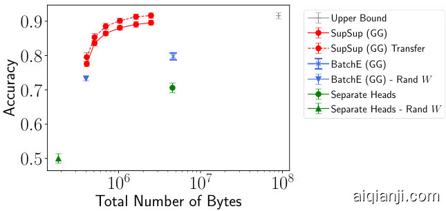
Figure 2: (left) Split Image net performance in Scenario GG. SupSup approaches upper bound performance with significantly fewer bytes. (right) Split CI FAR 100 performance in Scenario GG shown as mean and standard deviation over 5 seed and splits. SupSup outperforms similar size baselines and benefits from transfer.
| Algorithm | Avg Top 1 Accuracy (%) | Bytes |
| Upper Bound | 92.55 | 10222.81M |
| SupSup(GG) | 89.58 | 195.18M |
| 88.68 | 100.98M | |
| 86.37 | 65.50M | |
| BatchE (GG) | 81.50 | 124.99M |
| Single Model | 102.23M |
图 2: (左) Scenario GG 下的 Split ImageNet 性能表现。SupSup 以显著更少的字节数接近上限性能。(右) Scenario GG 下的 Split CIFAR-100 性能表现,显示为 5 次种子和分割的平均值及标准差。SupSup 优于相似规模的基线方法,并能从迁移中受益。
| 算法 | 平均 Top 1 准确率 (%) | 字节数 |
|---|---|---|
| 上限 | 92.55 | 10222.81M |
| SupSup(GG) | 89.58 | 195.18M |
| 88.68 | 100.98M | |
| 86.37 | 65.50M | |
| BatchE (GG) | 81.50 | 124.99M |
| 单模型 | 102.23M |
3 Methods
3 方法
In this section, we detail how SupSup leverages supermasks to learn thousands of sequential tasks without forgetting. We begin with easier settings where task identity is given and gradually move to more challenging scenarios where task identity is unavailable.
在本节中,我们将详细说明SupSup如何利用超掩码(supermask)在不遗忘的情况下学习数千个连续任务。我们从任务身份已知的简单场景开始,逐步过渡到更具挑战性的任务身份未知场景。
3.1 Preliminaries
3.1 预备知识
In a standard $\ell$ -way classification task, inputs $\mathbf{x}$ are mapped to a distribution p over output neurons ${1,...,\ell}$ . We consider the general case where $\mathbf{p}=f(\mathbf{x},W)$ for a neural network $f$ parameterized by $W$ and trained with a cross-entropy loss. In continual learning classification settings we have $k$ different $\ell$ -way classification tasks and the input size remains constant across tasks2.
在标准的 $\ell$ 类分类任务中,输入 $\mathbf{x}$ 被映射到输出神经元 ${1,...,\ell}$ 上的分布 p。我们考虑一般情况,其中 $\mathbf{p}=f(\mathbf{x},W)$,其中 $f$ 是由 $W$ 参数化的神经网络,并使用交叉熵损失进行训练。在持续学习分类设置中,我们有 $k$ 个不同的 $\ell$ 类分类任务,且输入大小在任务间保持不变[2]。
Zhou et al. [57] demonstrate that a trained binary mask (supermask) $M$ can be applied to a randomly weighted neural network, resulting in a subnetwork with good performance. As further explored by Ramanujan et al. [39], supermasks can be trained at similar compute cost to training weights while achieving performance competitive with weight training.
Zhou等[57]研究表明,训练好的二元掩码(supermask) $M$ 可应用于随机权重的神经网络,从而得到性能良好的子网络。Ramanujan等[39]进一步探索发现,训练supermask的计算成本与训练权重相当,同时能达到与权重训练相媲美的性能。
With supermasks, outputs are given by $\mathbf{p}=f\left(\mathbf{x},W\odot M\right)$ where $\odot$ denotes an element wise product. $W$ is kept frozen at its initialization: bias terms are 0 and other parameters in $W$ are $\pm c$ with equal probability and $c$ is the standard deviation of the corresponding Kaiming normal distribution [17]. This initialization is referred to as signed Kaiming constant by [39] and the constant $c$ may be different for each layer. For completeness we detail the Edge-Popup algorithm for training supermasks [39] in Section E of the appendix.
使用超掩码 (supermask) 时,输出由 $\mathbf{p}=f\left(\mathbf{x},W\odot M\right)$ 给出,其中 $\odot$ 表示逐元素乘积。 $W$ 保持初始化时的冻结状态:偏置项为 0, $W$ 中的其他参数以等概率取 $\pm c$ , $c$ 是对应 Kaiming 正态分布 [17] 的标准差。[39] 将这种初始化称为带符号 Kaiming 常量 (signed Kaiming constant),且每层的常量 $c$ 可能不同。为完整起见,我们在附录 E 节详细说明了训练超掩码的 Edge-Popup 算法 [39]。
3.2 Scenario GG: Task Identity Information Given During Train and Inference
3.2 场景GG:训练和推理期间给定任务身份信息
When task identity is known during training we can learn a binary mask $M^{i}$ per task. $M^{i}$ are the only parameters learned as the weights remain fixed. Given data from task $i$ , outputs are computed as
当任务身份在训练期间已知时,我们可以为每个任务学习一个二元掩码 $M^{i}$。$M^{i}$ 是唯一学习的参数,权重保持固定。给定任务 $i$ 的数据时,输出计算为
$$
\mathbf{p}=f\left(\mathbf{x},W\odot M^{i}\right)
$$
$$
\mathbf{p}=f\left(\mathbf{x},W\odot M^{i}\right)
$$
For each new task we can either initialize a new supermask randomly, or use a running mean of all supermasks learned so far. During inference for task $i$ we then use ${\dot{M}}^{i}$ . Figure 2 illustrates that in this scenario SupSup outperforms a number of baselines in accuracy on both Split CI FAR 100 and Split Image Net while requiring fewer bytes to store. Experiment details are in Section 4.1.
对于每个新任务,我们可以随机初始化一个新的超掩码,或者使用迄今为止学习到的所有超掩码的运行平均值。在任务 $i$ 的推理过程中,我们使用 ${\dot{M}}^{i}$。图 2 展示了在此场景下,SupSup 在 Split CI FAR 100 和 Split Image Net 上的准确率均优于多个基线方法,同时所需存储字节更少。实验细节见第 4.1 节。
3.3 Scenarios GNs & GNu : Task Identity Information Given During Train Only
3.3 场景 GNs 和 GNu:仅在训练期间提供任务身份信息
We now consider the case where input data comes from task $j$ , but this task information is unknown to the model at inference time. During training we proceed exactly as in Scenario GG, obtaining $k$ learned supermasks. During inference, we aim to infer task identity—correctly detect that the data belongs to task $j$ —and select the corresponding supermask $M^{j}$ .
我们现在考虑输入数据来自任务 $j$ 的情况,但模型在推理时并不知道这一任务信息。训练阶段我们完全按照场景 GG 的方式进行处理,获得 $k$ 个学习到的超级掩码。在推理阶段,我们的目标是推断任务身份(正确识别数据属于任务 $j$)并选择对应的超级掩码 $M^{j}$。
The SupSup procedure for task $\mathrm{ID}$ inference is as follows: first we associate each of the $k$ learned supermasks ${\bar{M}}^{i}$ with an coefficient $\alpha_ {i}\in[0,1]$ , initially set to $1/k$ . Each $\alpha_ {i}$ can be interpreted as the “belief” that supermask $M^{i}$ is the correct mask (equivalently the belief that the current unknown task is task $i^{\cdot}$ ). The model’s output is then be computed with a weighted superposition of all learned masks:
任务 $\mathrm{ID}$ 推断的 SupSup 过程如下:首先将 $k$ 个已学习的超掩码 ${\bar{M}}^{i}$ 分别与系数 $\alpha_ {i}\in[0,1]$ 关联,初始值设为 $1/k$。每个 $\alpha_ {i}$ 可解释为对超掩码 $M^{i}$ 是正确掩码的"置信度"(即认为当前未知任务是任务 $i^{\cdot}$ 的置信度)。模型输出随后通过所有已学习掩码的加权叠加计算得出:
$$
\mathbf{p}({\boldsymbol{\alpha}})=f\left(\mathbf{x},W\odot\left(\sum_ {i=1}^{k}\alpha_ {i}M^{i}\right)\right).
$$
$$
\mathbf{p}({\boldsymbol{\alpha}})=f\left(\mathbf{x},W\odot\left(\sum_ {i=1}^{k}\alpha_ {i}M^{i}\right)\right).
$$
The correct mask $M^{j}$ should produce a confident, low-entropy output [19]. Therefore, to recover the correct mask we find the coefficients $\alpha$ which minimize the output entropy $\mathcal{H}$ of $\mathbf p(\alpha)$ . One option is to perform gradient descent on $\alpha$ via
正确的掩码 $M^{j}$ 应产生一个置信度高、低熵的输出 [19]。因此,为了恢复正确的掩码,我们寻找使 $\mathbf p(\alpha)$ 的输出熵 $\mathcal{H}$ 最小化的系数 $\alpha$。一种方法是通过对 $\alpha$ 执行梯度下降来实现。
$$
\alpha\gets\alpha-\eta\nabla_ {\alpha}\mathcal{H}\left(\mathbf{p}\left(\alpha\right)\right)
$$
$$
\alpha\gets\alpha-\eta\nabla_ {\alpha}\mathcal{H}\left(\mathbf{p}\left(\alpha\right)\right)
$$
where $\eta$ is the step size, and $\alpha\mathbf{S}$ are re-normalized to sum to one after each update. Another option is to try each mask individually and pick the one with the lowest entropy output requiring $k$ forward passes. However, we want an optimization method with fixed sub-linear run time (w.r.t. the number of tasks $k$ ) which leads $\alpha$ to a corner of the probability simplex — i.e. $\alpha$ is 0 everywhere except for a single 1. We can then take the nonzero index to be the inferred task. To this end we consider the One-Shot and Binary algorithms.
其中 $\eta$ 是步长,$\alpha\mathbf{S}$ 在每次更新后会重新归一化为总和为1。另一种选择是单独尝试每个掩码,并选择具有最低熵输出的那个,这需要进行 $k$ 次前向传递。然而,我们需要一种具有固定次线性运行时间(相对于任务数 $k$)的优化方法,使得 $\alpha$ 达到概率单纯形的角落——即 $\alpha$ 除单个1外其余位置均为0。然后我们可以将非零索引作为推断的任务。为此,我们考虑单次尝试算法和二分算法。
One-Shot: The task is inferred using a single gradient. Specifically, the inferred task is given by
单样本 (One-Shot): 任务通过单次梯度推断得出。具体而言,推断出的任务由
$$
\underset{i}{\arg\operatorname*{max}}\left(-\frac{\partial\mathcal{H}\left(\mathbf{p}\left(\alpha\right)\right)}{\partial\alpha_ {i}}\right)
$$
$$
\underset{i}{\arg\operatorname*{max}}\left(-\frac{\partial\mathcal{H}\left(\mathbf{p}\left(\alpha\right)\right)}{\partial\alpha_ {i}}\right)
$$
as entropy is decreasing maximally in this coordinate. This algorithms corresponds to one step of the Frank-Wolfe algorithm [7], or one-step of gradient descent followed by softmax re-normalization with the step size $\eta$ approaching $\infty$ . Unless noted otherwise, $\mathbf{x}$ is a single image and not a batch.
当熵在该坐标系中最大程度减小时。该算法对应于Frank-Wolfe算法[7]的一步,或梯度下降后接步长$\eta$趋近于$\infty$的softmax重归一化。除非另有说明,$\mathbf{x}$指单张图像而非批量数据。
Binary: Resembling binary search, we infer task identity using an algorithm with $\log k$ steps. At each step we rule out half the tasks—the tasks corresponding to entries in the bottom half of $-\nabla_ {\alpha}\mathcal{H}\left(\mathbf{p}\left(\alpha\right)\right)$ . These are the coordinates in which entropy is minimally decreasing. A task $i$ is ruled out by setting $\alpha_ {i}$ to zero and at each step we re-normalize the remaining entries in $\alpha$ so that they sum to one. Pseudo-code for both algorithms may be found in Section A of the appendix.
二分法:类似于二分搜索,我们使用一个包含$\log k$步的算法来推断任务身份。每一步我们排除一半任务——即那些对应$-\nabla_ {\alpha}\mathcal{H}\left(\mathbf{p}\left(\alpha\right)\right)$下半部分条目的任务。这些是熵下降最少的坐标。通过将$\alpha_ {i}$设为零来排除任务$i$,并在每一步重新归一化$\alpha$中的剩余条目使其总和为一。两种算法的伪代码可在附录A部分找到。
Once the task is inferred the corresponding mask can be used as in Equation 1 to obtain class probabilities $\mathbf{p}$ . In both Scenario GNs and $\mathsf{G N u}$ the class probabilities $\mathbf{p}$ are returned. In GNu, $\mathbf{p}$ forms a distribution over the classes corresponding to the inferred task. Experiments solving thousands of tasks are detailed in Section 4.2.
一旦推断出任务,便可如公式1所示使用相应掩码获取类别概率$\mathbf{p}$。在场景GNs和$\mathsf{G N u}$中,均会返回类别概率$\mathbf{p}$。在GNu中,$\mathbf{p}$会形成与推断任务对应类别的概率分布。第4.2节详细阐述了解决数千项任务的实验。
3.4 Scenario NNs: No Task Identity During Training or Inference
3.4 场景神经网络:训练和推理期间无任务标识
Task inference algorithms from Scenario GN enable the extension of SupSup to Scenario NNs, where task identity is entirely unknown (even during training). If SupSup is uncertain about the current task identity, it is likely that the data do not belong to any task seen so far. When this occurs a new supermask is allocated, and $k$ (the number of tasks learned so far) is incremented.
场景GN中的任务推理算法使得SupSup能够扩展到场景NNs,其中任务身份完全未知(甚至在训练期间)。如果SupSup对当前任务身份不确定,很可能数据不属于迄今为止见过的任何任务。当这种情况发生时,会分配一个新的supermask,并且$k$(迄今为止学习的任务数量)递增。
We consider the One-Shot algorithm and say that SupSup is uncertain when performing task identity inference if $\nu=$ softmax $\left(-\nabla_ {\alpha}\mathcal{H}\left(\mathbf{p}\left(\alpha\right)\right)\right)$ is approximately uniform. Specifically, if $k\operatorname*{max}_ {i}\nu_ {i}<$ $1+\epsilon$ a new mask is allocated and $k$ is incremented. Otherwise mask arg $\operatorname*{max}_ {i}\nu_ {i}$ is used, which corresponds to Equation 4. We conduct experiments on learning up to 2500 tasks entirely without any task information, detailed in Section 4.3. Figure 4 shows that SupSup in Scenario NNs achieves comparable performance even to Scenario GNu.
我们考虑One-Shot算法,并认为当$\nu=$ softmax $\left(-\nabla_ {\alpha}\mathcal{H}\left(\mathbf{p}\left(\alpha\right)\right)\right)$近似均匀分布时,SupSup在执行任务身份推断时存在不确定性。具体而言,如果$k\operatorname*{max}_ {i}\nu_ {i}<$ $1+\epsilon$,则分配一个新掩码并递增$k$;否则使用arg $\operatorname*{max}_ {i}\nu_ {i}$对应的掩码,这与公式4相对应。我们在完全没有任何任务信息的情况下对学习多达2500个任务进行了实验,详见第4.3节。图4显示,在NNs场景中,SupSup的性能甚至可与GNu场景相媲美。
3.5 Beyond Linear Memory Dependence
3.5 超越线性内存依赖
Hopfield networks [20] implicitly encode a series of binary strings $\mathbf{z}^{i}\in{-1,1}^{d}$ with an associated energy function $\begin{array}{r}{E_ {\Psi}(\mathbf{z})=\sum_ {u v}\Psi_ {u v}\mathbf{z}_ {u}\mathbf{z}_ {v}}\end{array}$ . Each $\mathbf{z}^{i}$ is a minima of $E_ {\Psi}$ , and can be recovered with gradient descent. $\Psi\in\mathbb{R}^{d\times d}$ is initially 0, and to encode a new string $z^{i}$ , $\begin{array}{r}{\Psi\leftarrow\Psi+\frac{1}{d}{\bf z}^{i}{\bf z}^{i}}\end{array}$ .
Hopfield网络[20]通过能量函数$\begin{array}{r}{E_ {\Psi}(\mathbf{z})=\sum_ {u v}\Psi_ {u v}\mathbf{z}_ {u}\mathbf{z}_ {v}}\end{array}$隐式编码一系列二进制字符串$\mathbf{z}^{i}\in{-1,1}^{d}$。每个$\mathbf{z}^{i}$都是$E_ {\Psi}$的极小值点,可通过梯度下降恢复。初始时$\Psi\in\mathbb{R}^{d\times d}$为零矩阵,当编码新字符串$z^{i}$时,执行更新$\begin{array}{r}{\Psi\leftarrow\Psi+\frac{1}{d}{\bf z}^{i}{\bf z}^{i}}\end{array}$。
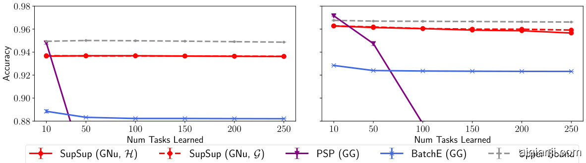
Figure 3: Using One-Shot to infer task identity, SupSup outperforms methods with access to task identity. Results shown for Permuted M NIST with LeNet 300-100 (left) and FC 1024-1024 (right).
图 3: 通过单样本推断任务身份,SupSup 优于已知任务身份的方法。结果显示为使用 LeNet 300-100 (左) 和 FC 1024-1024 (右) 的 Permuted MNIST。
We now consider implicitly encoding the masks in a fixed-size Hopfield network $\Psi$ for Scenario $\mathsf{G N u}$ . For a new task $i$ a new mask is learned. After training on task $i$ , this mask will be stored as an attractor in a fixed size Hopfield network. Given new data during inference we perform gradient descent on the Hopfield energy $E_ {\Psi}$ with the output entropy $\mathcal{H}$ to learn a new mask $\mathbf{m}$ . Minimizing $E_ {\Psi}$ will hopefully push $\mathbf{m}$ towards a mask learned during training while $\mathcal{H}$ will push $\mathbf{m}$ to be the correct mask. As $\Psi$ is quadratic in mask size, we will not mask the parameters $W$ . Instead we mask the output of every layer except the last, e.g. a network with one hidden layer and mask $\mathbf{m}$ is given by
我们现在考虑在固定大小的Hopfield网络$\Psi$中为场景$\mathsf{G N u}$隐式编码掩码。对于新任务$i$,将学习一个新的掩码。在任务$i$上训练后,该掩码将作为吸引子存储在固定大小的Hopfield网络中。在推理过程中给定新数据时,我们基于Hopfield能量$E_ {\Psi}$和输出熵$\mathcal{H}$进行梯度下降来学习新掩码$\mathbf{m}$。最小化$E_ {\Psi}$有望将$\mathbf{m}$推向训练期间学习的掩码,而$\mathcal{H}$将推动$\mathbf{m}$成为正确的掩码。由于$\Psi$在掩码大小上是二次的,我们将不对参数$W$进行掩码处理,而是对除最后一层外每一层的输出进行掩码。例如,具有一个隐藏层和掩码$\mathbf{m}$的网络表示为:
$$
f(\mathbf{x},\mathbf{m},W)=\mathtt{s o f t m a x}\left(W_ {2}^{\top}\left(\mathbf{m}\odot\sigma\left(W_ {1}^{\top}\mathbf{x}\right)\right)\right)
$$
$$
f(\mathbf{x},\mathbf{m},W)=\mathtt{s o f t m a x}\left(W_ {2}^{\top}\left(\mathbf{m}\odot\sigma\left(W_ {1}^{\top}\mathbf{x}\right)\right)\right)
$$
for non linearity $\sigma$ . The Hopfield network will then be a similar size as the base neural network. We refer to this method as HopSupSup and provide additional details in Section B.
对于非线性 $\sigma$,Hopfield 网络将与基础神经网络规模相当。我们将此方法称为 HopSupSup,并在 B 节提供了更多细节。
3.6 Superfluous Neurons an Entropy Alternative
3.6 冗余神经元 熵替代方案
Similar to previous methods [49], HopSupSup requires $\ell k$ output neurons in Scenario GNu. SupSup, however, is performing $\ell k$ -way classification without $\ell k$ output neurons. Given data during inference 1) the task is inferred and 2) the corresponding mask is used to obtain outputs p. The class probabilities $\mathbf{p}$ correspond to the classes for the inferred task, effectively reusing the neurons in the final layer.
与先前方法[49]类似,HopSupSup在GNu场景下需要$\ell k$个输出神经元。而SupSup则是在不配备$\ell k$个输出神经元的情况下执行$\ell k$路分类。在推理阶段给定数据时:1) 推断当前任务;2) 使用对应掩码获取输出p。类别概率$\mathbf{p}$对应推断任务的类别,从而高效复用最终层的神经元。
SupSup could use an output size of $\ell$ , though we find in practice that it helps significantly to add extra neurons to the final layer. Specifically we consider outputs $\mathbf{p}\in\mathbb{R}^{s}$ and refer to the neurons ${\ell{+}1,{\ldots},s}$ as superfluous neurons (s-neurons). The standard cross-entropy loss will push the values of s-neurons down throughout training. Accordingly, we consider an objective $\mathcal{G}$ which encourages the s-neurons to have large negative values and can be used as an alternative to entropy in Equation 4. Given data from task $j$ , mask $M^{j}$ will minimize the values of the s-neurons as it was trained to do. Other masks were also trained to minimize the values of the s-neurons, but not for data from task $j$ . In Lemma 1 of Section I we provide the exact form of $\mathcal{G}$ in code ( $\mathcal{G}=1$ ogsumexp $\mathbf{\eta}(\mathbf{p})$ with masked gradients for $\mathbf{p}_ {1},...,\mathbf{p}_ {\ell})$ and offer an alternative perspective on why $\mathcal{G}$ is effective — the gradient of $\mathcal{G}$ for all s-neurons exactly mirrors the gradient from the supervised training loss.
SupSup可以使用输出大小$\ell$,不过我们在实践中发现,在最后一层添加额外的神经元会有显著帮助。具体来说,我们考虑输出$\mathbf{p}\in\mathbb{R}^{s}$,并将神经元${\ell{+}1,{\ldots},s}$称为冗余神经元(s-neuron)。标准交叉熵损失会在整个训练过程中压低s-neuron的值。因此,我们考虑一个目标函数$\mathcal{G}$,它鼓励s-neuron具有较大的负值,并可作为方程4中熵的替代方案。给定任务$j$的数据时,掩码$M^{j}$会按照其训练目标最小化s-neuron的值。其他掩码虽然也经过训练来最小化s-neuron的值,但并非针对任务$j$的数据。在第一节的引理1中,我们提供了$\mathcal{G}$的代码实现形式( $\mathcal{G}=1$ ogsumexp $\mathbf{\eta}(\mathbf{p})$,其中对$\mathbf{p}_ {1},...,\mathbf{p}_ {\ell}$使用掩码梯度),并解释了$\mathcal{G}$的有效性原因——所有s-neuron的$\mathcal{G}$梯度完全镜像了监督训练损失的梯度。
4 Experiments
4 实验
4.1 Scenario GG: Task Identity Information Given During Train and Inference
4.1 场景GG:训练和推理期间给定任务身份信息
Datasets, Models & Training In this experiment we validate the performance of SupSup on Split CI FAR 100 and Split Image Net. Following Wen et al. [51], Split CI FAR 100 randomly partitions CIFAR100 [24] into 20 different 5-way classification problems. Similarly, Split Image Net randomly splits the ImageNet [5] dataset into 100 different 10-way classification tasks. Following [51] we use a ResNet-18 with fewer channels for Split CI FAR 100 and a standard ResNet-50 [18] for Split Image Net. The Edge-Popup algorithm from [39] is used to obtain supermasks for various sparsities with a layer-wise budget from [35]. We either initialize each new mask randomly (as in [39]) or use a running mean of all previous learned masks. This simple method of “Transfer” works very well, as illustrated by Figure 2. Additional training details and hyper parameters are provided in Section D.
数据集、模型与训练
在本实验中,我们在Split CIFAR 100和Split ImageNet上验证了SupSup的性能。遵循Wen等人[51]的方法,Split CIFAR 100将CIFAR100 [24]随机划分为20个不同的5分类问题。类似地,Split ImageNet将ImageNet [5]数据集随机划分为100个不同的10分类任务。按照[51]的设置,我们对Split CIFAR 100使用通道数较少的ResNet-18,对Split ImageNet使用标准ResNet-50 [18]。采用[39]提出的Edge-Popup算法,结合[35]的分层稀疏度预算,为不同稀疏度生成超掩码。新掩码的初始化方式包括随机初始化(如[39])或使用历史学习掩码的滑动平均值。如图2所示,这种简单的"迁移"方法效果显著。更多训练细节和超参数见附录D。

Figure 4: Learning 2500 tasks and inferring task identity using the One-Shot algorithm. Results for both the $\mathsf{G N u}$ and NNs scenarios with the LeNet 300-100 model using output size 500.
图 4: 使用单样本算法学习2500个任务并推断任务身份。展示了采用输出维度为500的LeNet 300-100模型时,$\mathsf{G N u}$和NNs两种场景下的结果。
Computation In Scenario GG, the primary advantage of SupSup from Mallya et al. [31] or Wen et al. [51] is that SupSup does not require the base model $W$ to be stored. Since $W$ is random it suffices to store only the random seed. For a fair comparison we also train BatchE [51] with random weights. The sparse supermasks are stored in the standard scipy.sparse. $\mathtt{c s c}^{3}$ format with 16 bit integers. Moreover, SupSup requires minimal overhead in terms of forwards pass compute. Element wise product by a binary mask can be implemented via memory access, i.e. selecting indices. Modern GPUs have very high memory bandwidth so the time cost of this operation is small with respect to the time of a forward pass. In particular, on a $1080\mathrm{Ti}$ this operation requires $\sim1%$ of the forward pass time for a ResNet-50, less than the overhead of BatchE (computation in Section D).
在场景GG的计算中,Mallya等人[31]或Wen等人[51]提出的SupSup主要优势在于无需存储基础模型$W$。由于$W$是随机生成的,仅需存储随机种子即可。为公平比较,我们也用随机权重训练了BatchE[51]。稀疏超掩码以16位整数形式存储于标准scipy.sparse.$\mathtt{c s c}^{3}$格式中。此外,SupSup在前向传播计算中的开销极小——通过内存访问(即索引选择)即可实现二进制掩码的逐元素乘积。现代GPU具备极高内存带宽,该操作耗时仅占ResNet-50前向传播时间的$\sim1%$(在1080Ti显卡上),低于BatchE的开销(计算细节见D节)。
Baselines In Figure 2, for “Separate Heads” we train different heads for each task using a trunk (all layers except the final layer) trained on the first task. In contrast “Separate Heads - Rand W” uses a random trunk. BatchE results are given with the trunk trained on the first task (as in [51]) and random weights $W$ . For “Upper Bound”, individual models are trained for each task. Furthermore, the trunk for task $i$ is trained on tasks $1,...,i$ . For “Lower Bound” a shared trunk of the network is trained continuously and a separate head is trained for each task. Since catastrophic forgetting occurs we omit “Lower Bound” from Figure 2 (the Split CI FAR 100 accuracy is $24.5%$ ).
基线方法
在图 2 中,"Separate Heads"方法针对每个任务使用在第一个任务上训练的主干网络(除最后一层外的所有层)训练不同的头部。相比之下,"Separate Heads - Rand W"使用随机初始化的主干网络。BatchE的结果给出了在第一个任务上训练的主干网络(如[51]所述)和随机权重$W$的情况。"Upper Bound"为每个任务单独训练模型,且任务$i$的主干网络是在任务$1,...,i$上训练的。"Lower Bound"方法持续训练共享的主干网络并为每个任务训练单独的头部,由于存在灾难性遗忘问题,图 2 中未展示该方法(Split CI FAR 100准确率为$24.5%$)。
4.2 Scenarios GNs & GNu: Task Identity Information Given During Train Only
4.2 场景 GNs 和 GNu:仅在训练期间提供任务身份信息
Our solutions for GNs and $\mathsf{G N u}$ are very similar. Because $\mathsf{G N u}$ is strictly more difficult, we focus on only evaluating in Scenario GNu. For relevant figures we provide a corresponding table in Section H.
我们对GN和$\mathsf{G N u}$的解决方案非常相似。由于$\mathsf{G N u}$严格更难,我们仅聚焦于在GNu场景下进行评估。相关图表数据请参阅附录H中的对应表格。
Datasets Experiments are conducted on Permuted M NIST, Rotated M NIST, and SplitMNIST. For Permuted M NIST [23], new tasks are created with a fixed random permutation of the pixels of MNIST. For Rotated M NIST, images are rotated by 10 degrees to form a new task with 36 tasks in total (similar to [4]). Finally SplitMNIST partitions MNIST into 5 different 2-way classification tasks, each containing consecutive classes from the original dataset.
数据集
实验在Permuted MNIST、Rotated MNIST和SplitMNIST上进行。对于Permuted MNIST [23],通过固定随机排列MNIST的像素来创建新任务。对于Rotated MNIST,图像旋转10度以形成新任务,共36个任务(类似于[4])。最后,SplitMNIST将MNIST划分为5个不同的二分类任务,每个任务包含原始数据集中连续的类别。
Training We consider two architectures: 1) a fully connected network with two hidden layers of size 1024 (denoted FC 1024-1024 and used in [4]) 2) the LeNet 300-100 architecture [25] as used in [8, 6]. For each task we train for 1000 batches of size 128 using the RMSProp optimizer [48] with learning rate 0.0001 which follows the hyper parameters of [4]. Supermasks are found using the algorithm of Mallya et al. [31] with threshold value 0. However, we initialize the real valued “scores” with Kaiming uniform as in [39]. Training the mask is not a focus of this work, we choose this method as it is fast and we are not concerned about controlling mask sparsity as in Section 4.1.
训练
我们考虑两种架构:
- 全连接网络,包含两个大小为1024的隐藏层(记为FC 1024-1024,用于[4])
- LeNet 300-100架构[25],如[8, 6]所用。
对于每个任务,我们使用RMSProp优化器[48](学习率0.0001,遵循[4]的超参数设置)训练1000个批次,每批次大小为128。超掩码(Supermasks)采用Mallya等人[31]的算法(阈值为0)生成,但实值"分数"初始化采用[39]中的Kaiming均匀分布。掩码训练并非本文重点,选择该方法因其速度快,且无需如第4.1节所述控制掩码稀疏度。
Evaluation At test time we perform inference of task identity once for each batch. If task is not inferred correctly then accuracy is 0 for the batch. Unless noted otherwise we showcase results for the most challenging scenario — when the task identity is inferred using a single image. We use “Full Batch” to indicate that all 128 images are used to infer task identity. Moreover, we experiment with both the the entropy $\mathcal{H}$ and $\mathcal{G}$ (Section 3.6) objectives to perform task identity inference.
评估
在测试阶段,我们对每批次数据执行一次任务身份推断。若任务识别错误,则该批次准确率为0。除非特别说明,我们均展示最具挑战性的场景结果——即使用单张图像推断任务身份。"Full Batch"表示使用全部128张图像进行任务身份推断。此外,我们分别采用熵目标$\mathcal{H}$和$\mathcal{G}$(第3.6节)进行任务身份推断实验。
Results Figure 4 illustrates that SupSup is able to sequentially learn 2500 permutations of MNIST— SupSup succeeds in performing 25,000-way classification. This experiment is conducted with the One-Shot algorithm (requiring one gradient computation) using single images to infer task identity. The same trends hold in Figure 3, where SupSup outperforms methods which operate in Scenario GG by using the One-Shot algorithm to infer task identity. In Figure 3, output sizes of 100 and 500 are respectively used for LeNet 300-100 and FC 1024-1024. The left hand side of Figure 5 illustrates that SupSup is able to infer task identity even when tasks are similar—SupSup is able to distinguish between rotations of 10 degrees. Since this is a more challenging problem, we use a full batch and the Binary algorithm to perform task identity inference. Figure 7 (appendix) shows that for HopSupSup on SplitMNIST, the new mask m converges to the correct supermask in $<30$ gradient steps.
结果
图4表明,SupSup能够顺序学习2500种MNIST排列组合——成功实现了25,000类分类。该实验采用单样本(One-Shot)算法(仅需一次梯度计算),通过单张图像推断任务标识。图3中呈现相同趋势:当使用单样本算法推断任务标识时,SupSup在GG场景下的表现优于其他方法。图3中,LeNet 300-100和FC 1024-1024分别采用100和500的输出维度。图5左侧显示,即使任务相似(如区分10度旋转差异),SupSup仍能准确推断任务标识。由于该问题更具挑战性,我们使用完整批次数据和二元(Binary)算法进行任务标识推断。图7(附录)表明,在SplitMNIST数据集上,HopSupSup的新掩码m可在$<30$次梯度步长内收敛至正确的超掩码(supermask)。

Figure 5: (left) Testing the FC 1024-1024 model on Rotated M NIST. SupSup uses Binary to infer task identity with a full batch as tasks are similar (differing by only 10 degrees). (right) The OneShot algorithm can be used to infer task identity for BatchE [51]. Experiment conducted with FC 1024-1024 on Permuted M NIST using an output size of 500, shown as mean and stddev over 3 runs.
图 5: (左) 在旋转MNIST上测试FC 1024-1024模型。由于任务相似(仅相差10度),SupSup使用Binary方法通过完整批次推断任务标识。(右) OneShot算法可用于推断BatchE [51]的任务标识。实验在排列MNIST上使用FC 1024-1024模型进行,输出尺寸为500,结果显示为3次运行的平均值和标准差。
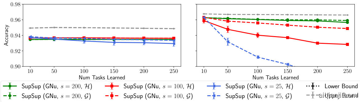
Figure 6: The effect of output size $s$ on SupSup performance using the One-Shot algorithm. Results shown for Permuted M NIST with LeNet 300-100 (left) and FC 1024-1024 (right).
图 6: 输出尺寸 $s$ 对使用 One-Shot 算法的 SupSup 性能影响。结果显示为使用 LeNet 300-100 (左) 和 FC 1024-1024 (右) 的 Permuted MNIST。
Baselines & Ablations Figure 5 (left) shows that even in Scenario GNu, SupSup is able to outperform PSP [4] and BatchE [51] in Scenario GG—methods using task identity. We compare SupSup in $\mathsf{G N u}$ with methods in this strictly easier scenario as they are more competitive. For instance, [49] considers sequential learning problems with only 5-10 tasks. SupSup, after sequentially learning 250 permutations of MNIST, outperforms all non-replay methods from [3] in the GNu scenario after they have learned only 10 permutations of MNIST with a similar network. In GNu, Online EWC achieves $33.88%$ & SI achieves $29.31%$ on 10 permutations of MNIST [49] while SupSup achieves $94.91%$ accuracy after 250 permutations (see Table 5 in [49] vs. Table 7).
基线方法与消融实验
图5(左)显示即使在GNu场景下,SupSup也能在GG场景中超越使用任务标识的PSP[4]和BatchE[51]方法。我们将$\mathsf{G N u}$场景下的SupSup与这个严格更简单场景中的方法进行比较,因为它们更具竞争力。例如,[49]研究的是仅含5-10个任务的序列学习问题。在连续学习250个MNIST排列后,SupSup在GNu场景中的表现优于[3]中所有非回放方法——后者仅用相似网络学习了10个MNIST排列。在GNu场景中,Online EWC在10个MNIST排列上达到$33.88%$,SI达到$29.31%$[49],而SupSup在250个排列后准确率达到$94.91%$(对比[49]表5与表7)。
In Figure 5 (right) we equip BatchE with task inference using our One-Shot algorithm. Instead of attaching a weight $\alpha_ {i}$ to each supermask, we attach a weight $\alpha_ {i}$ to each rank-one matrix [51]. Moreover, in Section C of the appendix we augment BatchE to perform task-inference using large batch sizes. “Upper Bound” and “Lower Bound” are the same as in Section 4.1. Moreover, Figure 6 illustrates the importance of output size. Further investigation of this phenomena is provided by Section 3.6 and Lemma 1 of Section I.
在图5(右)中,我们使用One-Shot算法为BatchE配备了任务推断功能。不同于为每个超掩码分配权重$\alpha_ {i}$,我们改为为每个秩一矩阵[51]分配权重$\alpha_ {i}$。此外,在附录C节中,我们增强了BatchE以支持大批量规模下的任务推断。"上界"与"下界"的定义与4.1节保持一致。图6则说明了输出维度的重要性,该现象的深入分析详见3.6节及附录I节的引理1。
4.3 Scenario NNs: No Task Identity During Training or Inference
4.3 场景NNs:训练和推理期间无任务标识
For the NNs Scenario we consider Permuted M NIST and train on each task for 1000 batches (the model does not have access to this iteration number). Every 100 batches the model must choose to allocate a new mask or pick an existing mask using the criteria from Section 3.4 $(\epsilon=2^{-3}$ ). Figure 4 illustrates that without access to any task identity (even during training) SupSup is able to learn thousands of tasks. However, a final dip is observed as a budget of 2500 supermasks total is enforced.
在神经网络(NNs)场景中,我们考虑使用排列后的MNIST数据集,并在每个任务上训练1000个批次(模型无法获知此迭代次数)。每100个批次,模型必须根据3.4节的标准$(\epsilon=2^{-3})$选择分配新掩码或选取现有掩码。图4表明,在没有任何任务标识(即使在训练期间)的情况下,SupSup仍能学习数千个任务。然而,由于强制执行了2500个超级掩码的总预算限制,最终出现了性能下降。
5 Conclusion
5 结论
Supermasks in Superposition (SupSup) is a flexible and compelling model applicable to a wide range of scenarios in Continual Learning. SupSup leverages the power of sub networks [57, 39, 31], and gradient-based optimization to infer task identity when unknown. SupSup achieves state-ofthe-art performance on Split Image Net when given task identity, and performs well on thousands of permutations and almost indiscernible rotations of MNIST without any task information.
叠加超掩码(SupSup)是一种灵活且强大的模型,适用于持续学习中的多种场景。该模型通过利用子网络[57,39,31]的优势和基于梯度的优化,在任务身份未知时进行推断。在给定任务身份的情况下,SupSup在Split Image Net上实现了最先进的性能;在没有任何任务信息时,该模型也能在MNIST数据集的数千种排列组合和几乎无法辨别的旋转图像上表现优异。
We observe limitations in applying SupSup with task identity inference to non-uniform and more challenging problems. Task inference fails when models are not well calibrated—are overly confident for the wrong task. As future work, we hope to explore automatic task inference with more calibrated models [14], as well as circumventing calibration challenges by using optimization objectives such as self-supervision [16] and energy based models [13]. In doing so, we hope to tackle large-scale problems in Scenarios GN and NNs.
我们观察到,在将SupSup与任务身份推断应用于非均匀且更具挑战性的问题时存在局限性。当模型校准不佳(对错误任务过度自信)时,任务推断会失败。作为未来工作,我们希望探索使用更校准的模型进行自动任务推断[14],并通过自监督[16]和基于能量的模型[13]等优化目标规避校准挑战。借此,我们希望能解决GN和NNs场景中的大规模问题。
Broader Impact
更广泛的影响
A goal of continual learning is to solve many tasks with a single model. However, it is not exactly clear what qualifies as a single model. Therefore, a concrete objective has become to learn many tasks as efficiently as possible. We believe that SupSup is a useful step in this direction. However, there are consequences to more efficient models, both positive and negative.
持续学习的一个目标是用单一模型解决多项任务。然而,对于何为单一模型尚无明确定义。因此,更具体的目标已转变为尽可能高效地学习多个任务。我们认为SupSup是迈向该目标的有益尝试。但高效模型会带来双重影响 (positive and negative) 。
We begin with the positive consequences:
我们从积极影响开始:
We would also like to highlight and discuss the negative consequences of models which can efficiently learn many tasks, and efficient models in general. When models are more efficient, they are also more available and less subject to regular iz ation and study as a result. For instance, when a high-impact model is released by an institution it will hopefully be accompanied by a Model Card [34] analyzing the bias and intended use of the model. By contrast, if anyone is able to train a powerful model this may no longer be the case, resulting in a proliferation of models with harmful biases or intended use. Taking the United States for instance, bias can be harmful as models show disproportionately more errors for already marginalized groups [2], furthering existing and deeply rooted structural racism.
我们还需强调并讨论能高效学习多种任务的模型以及高效模型普遍存在的负面影响。当模型效率提高时,其可获得性也随之增强,但相应的规范审查与研究却可能减少。例如,当机构发布高影响力模型时,理想情况下应附带分析模型偏见和预期用途的模型卡片(Model Card) [34];而若任何人都能训练强大模型,这种规范可能失效,导致带有有害偏见或用途的模型泛滥。以美国为例,当模型对已被边缘化的群体显示出不成比例的高错误率时[2],这种偏见会加剧根深蒂固的结构性种族主义。
Acknowledgments
致谢
We thank Gabriel Ilharco Magalhães and Sarah Pratt for helpful comments. For valuable conversations we also thank Tim Dettmers, Kiana Ehsani, Ana Marasovic, Suchin Gururangan, Zoe Steine-Hanson, Connor Shorten, Samir Yitzhak Gadre, Samuel McKinney and Kishanee Hath thot uwe gama. This work is in part supported by NSF IIS 1652052, IIS 17303166, DARPA N66001-19-2-4031, DARPA W911NF-15-1-0543 and gifts from Allen Institute for Artificial Intelligence. Additional revenues: co-authors had employment with the Allen Institute for AI.
我们感谢 Gabriel Ilharco Magalhães 和 Sarah Pratt 提出的宝贵意见。同时感谢 Tim Dettmers、Kiana Ehsani、Ana Marasovic、Suchin Gururangan、Zoe Steine-Hanson、Connor Shorten、Samir Yitzhak Gadre、Samuel McKinney 以及 Kishanee Hath thot uwe gama 进行的有益讨论。本研究部分得到了 NSF IIS 1652052、IIS 17303166、DARPA N66001-19-2-4031、DARPA W911NF-15-1-0543 以及艾伦人工智能研究所 (Allen Institute for Artificial Intelligence) 的资助支持。其他收入来源:部分合著者受雇于艾伦人工智能研究所。
References
参考文献
[1] Yoshua Bengio, Nicolas L Roux, Pascal Vincent, Olivier Delalleau, and Patrice Marcotte. Convex neural networks. In Advances in neural information processing systems, pages 123–130, 2006.
[1] Yoshua Bengio, Nicolas L Roux, Pascal Vincent, Olivier Delalleau, and Patrice Marcotte. 凸神经网络. In Advances in neural information processing systems, pages 123–130, 2006.
| Algorithm 1 One-Shot( f, x, W, k, {Mi}=1, H) | |
| 1: Q← [ 1飞 引 | InitializeO |
| 2: p←f x, W @ i=1 QiM | Superimposedoutput |
| H(p) 3:return arg max dai | Return coordinate for which objective maximally decreasing |
算法 1 One-Shot( f, x, W, k, {Mi}=1, H)
| 1: Q← [ 1飞 引 | 初始化O |
| 2: p←f x, W @ i=1 QiM | 叠加输出 |
| H(p) 3:return arg max dai | 返回目标函数最大下降的坐标 |
A Algorithm pseudo-code
A 算法伪代码
Algorithms 1 and 2 respectively provide pseudo-code for the One-Shot and Binary algorithms detailed in Section 3.3. Both aim to infer the task $j\in{1,...,k}$ associated with input data $\mathbf{x}$ by minimizing the objective $\mathcal{H}$ .
算法1和算法2分别提供了第3.3节中详细描述的One-Shot和Binary算法的伪代码。两者都旨在通过最小化目标函数$\mathcal{H}$来推断与输入数据$\mathbf{x}$相关的任务$j\in{1,...,k}$。
B Extended Details for HopSupSup
B HopSupSup 扩展详情
This section provides further details and experiments for HopSupSup (introduced in Section 3.5). HopSupSup provides a method for storing the growing set of supermasks in a fixed size reservoir instead of explicitly storing each mask.
本节将详细介绍HopSupSup (见3.5节) 的更多细节与实验。HopSupSup提出了一种在固定容量的存储池中保存不断增长的超级掩码(supermask)集合的方法,而非显式存储每个掩码。
B.1 Training
B.1 训练
Recall that HopSupSup operates in Scenario GNu and so task identity is known during training. Instead of explicitly storing each mask, we will instead store two fixed sized variables $\Psi$ and $\mu$ which are both initially 0. The weights of the Hopfield network are $\Psi$ and $\mu$ stores a running mean of all masks learned so far. For a new task $k$ we use the same algorithm as in Section 4.2 to learn a binary mask $\mathbf{m}^{i}$ which performs well for task $k$ . Since Hopfield networks consider binary strings in ${-1,1}^{d}$ and we use masks $\mathbf{m}^{i}\in{0,1}^{d}$ we will consider $\mathbf{z}^{k}=2\mathbf{m}^{k}-1$ . In practice we then update $\Psi$ and $\mu$ as
回想一下,HopSupSup在GNu场景下运行,因此在训练期间任务身份是已知的。我们不会显式存储每个掩码,而是存储两个固定大小的变量$\Psi$和$\mu$,它们初始值均为0。Hopfield网络的权重为$\Psi$,而$\mu$存储迄今为止学习的所有掩码的滑动平均值。对于新任务$k$,我们使用与第4.2节相同的算法学习一个二元掩码$\mathbf{m}^{i}$,该掩码在任务$k$上表现良好。由于Hopfield网络考虑的是${-1,1}^{d}$中的二元字符串,而我们使用的掩码是$\mathbf{m}^{i}\in{0,1}^{d}$,因此我们将$\mathbf{z}^{k}=2\mathbf{m}^{k}-1$。实际操作中,我们随后更新$\Psi$和$\mu$如下:
$$
\Psi\leftarrow\Psi+\frac{1}{d}\left(\mathbf{z}^{k}\mathbf{z}^{k^{\top}}-\mathbf{z}^{k}\left(\Psi\mathbf{z}^{k}\right)^{\top}-\left(\Psi\mathbf{z}^{k}\right)\mathbf{z}^{k^{\top}}-\mathrm{Id}\right),\qquad\mu\leftarrow\frac{k-1}{k}\mu+\frac{1}{k}\mathbf{z}^{k}
$$
$$
\Psi\leftarrow\Psi+\frac{1}{d}\left(\mathbf{z}^{k}\mathbf{z}^{k^{\top}}-\mathbf{z}^{k}\left(\Psi\mathbf{z}^{k}\right)^{\top}-\left(\Psi\mathbf{z}^{k}\right)\mathbf{z}^{k^{\top}}-\mathrm{Id}\right),\qquad\mu\leftarrow\frac{k-1}{k}\mu+\frac{1}{k}\mathbf{z}^{k}
$$
where Id is the identity matrix. This update rule for $\Psi$ is referred to as the Storkey learning rule [46] and is more expressive than the alternative—the Hebbian rule $\Psi \leftarrow \Psi + \frac{1}{d} \mathbf{z}^{k} (\mathbf{z}^{k})^{\top}$ [20] provided for brevity in Section 3.3. With either update rules the learned $\mathbf{z}^{i}$ will be a minimizer of the Hopfield energy $\begin{array}{r}{E_ {\Psi}(\mathbf{z})=\sum_ {u v}\Psi_ {u v}\mathbf{z}_ {u}\mathbf{z}_ {v}}\end{array}$ .
其中 Id 是单位矩阵。$\Psi$ 的这种更新规则被称为 Storkey 学习规则 [46],比另一种 Hebbian 规则 $\Psi \leftarrow \Psi + \frac{1}{d} \mathbf{z}^{k} (\mathbf{z}^{k})^{\top}$ [20] 更具表现力,后者在第 3.3 节中为简洁起见提供。无论采用哪种更新规则,学习到的 $\mathbf{z}^{i}$ 都将是 Hopfield 能量 $\begin{array}{r}{E_ {\Psi}(\mathbf{z})=\sum_ {u v}\Psi_ {u v}\mathbf{z}_ {u}\mathbf{z}_ {v}}\end{array}$ 的最小化器。
B.2 Inference
B.2 推理
During inference we receive data $\mathbf{x}$ from some task $j$ , but this task information is not given to the model. HopSupSup first initializes a new binary string $\mathbf{z}$ with $\mu$ . Next, HopSupSup uses gradient descent to minimize the Hopfield energy in conjunction with the output entropy using mask $\begin{array}{r}{\mathbf{\bar{m}}=\frac{1}{2}\mathbf{z}+1}\end{array}$ , a process we refer to as Hopfield Recovery. Minimizing the energy will hopefully push m (equivalently $\mathbf{z}$ ) towards a mask learned during training and minimizing the entropy will hopefully push m towards the correct mask $\mathbf{m}^{j}$ . We may then use the recovered mask to compute the network output.
在推理过程中,我们接收来自任务 $j$ 的数据 $\mathbf{x}$,但模型并未获得该任务信息。HopSupSup首先用 $\mu$ 初始化一个新的二进制字符串 $\mathbf{z}$。接着,HopSupSup通过梯度下降最小化霍普菲尔德能量 (Hopfield energy) 和输出熵,使用的掩码为 $\begin{array}{r}{\mathbf{\bar{m}}=\frac{1}{2}\mathbf{z}+1}\end{array}$,这一过程称为霍普菲尔德恢复 (Hopfield Recovery)。最小化能量有望将 m(等价于 $\mathbf{z}$)推向训练期间学习到的掩码,而最小化熵则有望将 m 推向正确的掩码 $\mathbf{m}^{j}$。之后,我们可使用恢复的掩码计算网络输出。
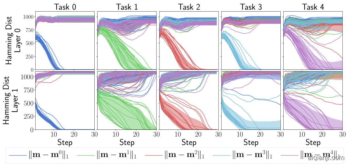
Figure 7: During Hopfield Recovery the new mask m converges to the correct mask learned during training. Note that $\mathbf{m}^{i}$ denotes the mask learned for task $i$ .
图 7: Hopfield恢复过程中,新掩码m收敛至训练时学得的正确掩码。注意$\mathbf{m}^{i}$表示任务$i$对应的学得掩码。
In practice we use one pass through the evaluation set (with batch size 64, requiring $T\approx30$ steps) to recover a mask and another to perform evaluation with the recovered mask. When recovering the mask we gradually increase the strength of the Hopfield term and decrease the strength of the entropy term. Otherwise the Hopfield term initially pulls $\mathbf{z}$ in the wrong direction or the final $\mathbf{z}$ does not lie at a minimum of $E_ {\Psi}$ . For step $t\in{1,...,T}$ , and constant $\gamma$ we use the objective $\mathcal{I}$ as
实践中,我们通过评估集进行一次遍历(批大小为64,需要约 $T\approx30$ 步)来恢复掩码,再用另一次遍历基于恢复的掩码进行评估。在恢复掩码时,我们逐步增强Hopfield项的强度并降低熵项的强度。否则,Hopfield项最初会将 $\mathbf{z}$ 拉向错误方向,或最终 $\mathbf{z}$ 未处于 $E_ {\Psi}$ 的极小值点。对于第 $t\in{1,...,T}$ 步和常数 $\gamma$,我们使用目标函数 $\mathcal{I}$ 如下:
$$
\mathcal{I}(\mathbf{z},t)=\frac{\gamma t}{T}E_ {\Psi}(\mathbf{z})+\left(1-\frac{t}{T}\right)\mathcal{H}\left(\mathbf{p}\right)
$$
$$
\mathcal{I}(\mathbf{z},t)=\frac{\gamma t}{T}E_ {\Psi}(\mathbf{z})+\left(1-\frac{t}{T}\right)\mathcal{H}\left(\mathbf{p}\right)
$$
where $\mathbf{p}$ denotes the output using mask $\begin{array}{r}{{\bf m}=\frac{1}{2}{\bf z}+1}\end{array}$ .
其中 $\mathbf{p}$ 表示使用掩码 $\begin{array}{r}{{\bf m}=\frac{1}{2}{\bf z}+1}\end{array}$ 的输出。
Figure 7 illustrates that after approximately 30 steps of gradient descent on z using objective $\mathcal{I}$ , the mask $\begin{array}{r}{{\bf m}=\frac{1}{2}{\bf z}+1}\end{array}$ converges to the correct mask learned during training. This experiment is conducted for 20 different random seeds on SplitMNIST (see Section 4.2) training for 1 epoch per task. Evaluation with the recovered mask for each seed is then given by Figure 8. As expected, when the correct mask is successfully recovered, accuracy matches directly using the correct mask. For hyper parameters we set $\gamma=1.{\dot{5}}\cdot10^{-3}$ and perform gradient descent during Hopfield recovery with learning rate $0.5\cdot10^{3}$ , momentum 0.9, and weight decay $10^{-4}$ .
图 7: 展示了在目标函数 $\mathcal{I}$ 下对 z 进行约 30 步梯度下降后,掩码 $\begin{array}{r}{{\bf m}=\frac{1}{2}{\bf z}+1}\end{array}$ 会收敛至训练期间学习到的正确掩码。本实验在 SplitMNIST (见第 4.2 节) 上采用 20 个不同随机种子进行,每个任务训练 1 个周期。图 8 给出了使用各种子恢复掩码后的评估结果。正如预期,当成功恢复正确掩码时,其准确率与直接使用正确掩码完全一致。超参数设置为 $\gamma=1.{\dot{5}}\cdot10^{-3}$ ,并在 Hopfield 恢复过程中采用学习率 $0.5\cdot10^{3}$ 、动量 0.9 和权重衰减 $10^{-4}$ 进行梯度下降。
B.3 Network Architecture
B.3 网络架构
Let BN denote non-affine batch normalization [21], i.e. batch normalization with no learned parameters. Also recall that we are masking layer outputs instead of weights, and the weights still remain fixed (see Section 3.5). Therefore, with mask $\mathbf{m}=(\mathbf{m}_ {1},\mathbf{m}_ {2})$ and weights $W\bar{=}(W_ {1},W_ {2},W_ {3})$ we compute outputs as
设BN表示非仿射批量归一化 (batch normalization) [21],即没有可学习参数的批量归一化。同时请注意,我们是对层输出进行掩码而非权重,且权重仍保持固定(参见第3.5节)。因此,给定掩码$\mathbf{m}=(\mathbf{m}_ {1},\mathbf{m}_ {2})$和权重$W\bar{=}(W_ {1},W_ {2},W_ {3})$,输出计算方式为
$$
f(\mathbf{x},\mathbf{m},W)=\mathtt{s o f t m a x}\left(W_ {3}^{\top}\sigma\left(\mathbf{m}_ {2}\odot\mathtt{B N}\left(W_ {2}^{\top}\sigma\left(\mathbf{m}_ {1}\odot\mathtt{B N}\left(W_ {1}^{\top}\mathbf{x}\right)\right)\right)\right)\right)
$$
$$
f(\mathbf{x},\mathbf{m},W)=\mathtt{s o f t m a x}\left(W_ {3}^{\top}\sigma\left(\mathbf{m}_ {2}\odot\mathtt{B N}\left(W_ {2}^{\top}\sigma\left(\mathbf{m}_ {1}\odot\mathtt{B N}\left(W_ {1}^{\top}\mathbf{x}\right)\right)\right)\right)\right)
$$
where $\sigma$ denotes the Swish non linearity [38]. Without masking or normalization $f$ is a fully connected network with two hidden layers of size 2048. We also note that HopSupSup requires 10 output neurons for SplitMNIST in Scenario $\mathsf{G N u}$ , and the composition of non-affine batch normalization with a binary mask was inspired by BatchNets [9].
其中$\sigma$表示Swish非线性激活函数[38]。在不使用掩码或归一化的情况下,$f$是一个具有两个2048维度隐藏层的全连接网络。我们还需指出,在场景$\mathsf{G N u}$下的SplitMNIST任务中,HopSupSup需要10个输出神经元,其将非仿射批量归一化与二元掩码组合的设计灵感源自BatchNets[9]。
C Augmenting BatchE For Scnario GNu
C 增强 BatchE 以适用于场景 GNu
In Section 4.2 we demonstrate that BatchE [51] is able to infer task identity using the One-Shot algorithm. In this section we show that, equipped with $\mathcal{H}$ from Section 3, BatchE can also infer task identity by using a large batch size. We refer to this method as Augmented BatchE (ABatchE).
在4.2节中我们证明了BatchE [51]能够通过One-Shot算法推断任务身份。本节将展示,当配备第3节中的$\mathcal{H}$时,BatchE还能通过大批量尺寸推断任务身份。我们将该方法称为增强型BatchE (ABatchE)。
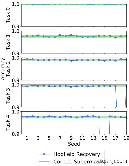
Figure 8: Evaluating (with 20 random seeds) on SplitMNIST after finding a mask with Hopfield Recovery. Average accuracy is $97.43%$ .
图 8: 使用Hopfield恢复找到掩码后在SplitMNIST上的评估(采用20个随机种子)。平均准确率为$97.43%$。

Figure 9: Continual learning scenarios detailed in Table 1 represented in a tree graph, as in [55].
图 9: 表 1 中详述的持续学习场景以树状图形式呈现,如 [55] 所示。
For clarity we describe ABatchE for one linear layer, i.e. we describe the application of ABatchE to
为清晰起见,我们针对单个线性层描述ABatchE,即阐述ABatchE在
$$
f(\mathbf{x},W)=\mathtt{s o f t m a x}\left(W^{\top}\mathbf{x}\right)
$$
$$
f(\mathbf{x},W)=\mathtt{s o f t m a x}\left(W^{\top}\mathbf{x}\right)
$$
for input data $\mathbf{x}\in\mathbb{R}^{m}$ and weights $W\in\mathbb{R}^{m\times n}$ . In BatchE [51], $W$ is trained on the first task then frozen. For task $i$ BatchE learns “fast weights” $r_ {i}\in\mathbb{R}^{m}$ , $s_ {i}\in\mathbb{R}^{n}$ and outputs are computed via
对于输入数据 $\mathbf{x}\in\mathbb{R}^{m}$ 和权重 $W\in\mathbb{R}^{m\times n}$ ,在 BatchE [51] 中,$W$ 在第一个任务上训练后冻结。对于任务 $i$,BatchE 学习"快速权重" $r_ {i}\in\mathbb{R}^{m}$ 和 $s_ {i}\in\mathbb{R}^{n}$,并通过以下方式计算输出:
$$
f(\mathbf{x},W)=\mathtt{s o f t m a x}\left(\left(W\odot r_ {i}s_ {i}^{\top}\right)^{\top}\mathbf{x}\right).
$$
$$
f(\mathbf{x},W)=\mathtt{softmax}\left(\left(W\odot r_ {i}s_ {i}^{\top}\right)^{\top}\mathbf{x}\right).
$$
Wen et al. [51] further demonstrate that Equation 10 can be vectorized as
Wen等[51]进一步证明了公式10可向量化为
$$
f(\mathbf{x},W)=\operatorname{softmax}\left(\left(W^{\top}\left(\mathbf{x}\odot r_ {i}\right)\right)\odot s_ {i}\right)
$$
$$
f(\mathbf{x},W)=\operatorname{softmax}\left(\left(W^{\top}\left(\mathbf{x}\odot r_ {i}\right)\right)\odot s_ {i}\right)
$$
or, for a batch of data X ∈ Rb×m,
或者,对于一批数据 X ∈ Rb×m,
$$
f(X,W)=\mathsf{s o f t m a x}\left(\left(\left(X\odot R_ {i}^{b}\right)W\right)\odot S_ {i}^{b}\right).
$$
$$
f(X,W)=\mathsf{s o f t m a x}\left(\left(\left(X\odot R_ {i}^{b}\right)W\right)\odot S_ {i}^{b}\right).
$$
In Equation 12, $R_ {i}^{b}\in\mathbb{R}^{b\times m}$ is a matrix where each of the $b$ rows is $r_ {i}$ (likewise $S_ {i}^{b}\in\mathbb{R}^{b\times n}$ is a matrix where each of the $b$ rows is $s_ {i}$ ).
在公式12中,$R_ {i}^{b}\in\mathbb{R}^{b\times m}$ 是一个矩阵,其中 $b$ 行的每一行都是 $r_ {i}$ (同理 $S_ {i}^{b}\in\mathbb{R}^{b\times n}$ 是一个矩阵,其中 $b$ 行的每一行都是 $s_ {i}$ )。
As in Section 3.3 we now consider the case where data $X\in\mathbb{R}^{b\times m}$ comes from task $j$ but this information is not known to the model. For ABatchE we repeat the data $k$ times, where $k$ is the number of tasks learned so far, and use different “fast weights” for each repetiton. Specifically, we consider repeated data $\tilde{\boldsymbol X}\in\mathbb R^{b\boldsymbol k\times m}$ and augmented matricies $\tilde{R}\in\mathbb R^{b k\times m}$ and $\tilde{S}\in\mathbb{R}^{b k\times n}$ given by
如第3.3节所述,我们现在考虑数据$X\in\mathbb{R}^{b\times m}$来自任务$j$但模型未知该信息的情况。对于ABatchE方法,我们将数据重复$k$次($k$表示当前已学习的任务数量),并为每次重复使用不同的"快速权重"。具体而言,我们使用重复数据$\tilde{\boldsymbol X}\in\mathbb R^{b\boldsymbol k\times m}$以及增广矩阵$\tilde{R}\in\mathbb R^{b k\times m}$和$\tilde{S}\in\mathbb{R}^{b k\times n}$进行处理
$$
\tilde{X}=\left[\begin{array}{c}{{X}}\ {{X}}\ {{\vdots}}\ {{X}}\end{array}\right],\tilde{R}=\left[\begin{array}{c}{{R_ {1}^{b}}}\ {{R_ {2}^{b}}}\ {{\vdots}}\ {{R_ {k}^{b}}}\end{array}\right],\tilde{S}=\left[\begin{array}{c}{{S_ {1}^{b}}}\ {{S_ {2}^{b}}}\ {{\vdots}}\ {{S_ {k}^{b}}}\end{array}\right].
$$
$$
\tilde{X}=\left[\begin{array}{c}{{X}}\ {{X}}\ {{\vdots}}\ {{X}}\end{array}\right],\tilde{R}=\left[\begin{array}{c}{{R_ {1}^{b}}}\ {{R_ {2}^{b}}}\ {{\vdots}}\ {{R_ {k}^{b}}}\end{array}\right],\tilde{S}=\left[\begin{array}{c}{{S_ {1}^{b}}}\ {{S_ {2}^{b}}}\ {{\vdots}}\ {{S_ {k}^{b}}}\end{array}\right].
$$
Outputs are then computed as
输出结果计算为
$$
f(X,W)=\mathtt{s o f t m a x}\left(\left(\left(\tilde{X}\odot\tilde{R}\right)W\right)\odot\tilde{S}\right)
$$
$$
f(X,W)=\mathtt{s o f t m a x}\left(\left(\left(\tilde{X}\odot\tilde{R}\right)W\right)\odot\tilde{S}\right)
$$
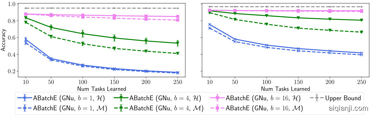
Figure 10: Testing ABatchE on Permuted M NIST with LeNet 300-100 (left) and FC 1024-1024 (right) with output size 100.
图 10: 在排列后的MNIST数据集上测试ABatchE,使用LeNet 300-100 (左) 和FC 1024-1024 (右) 网络结构,输出维度为100。
where the $b$ rows $(b i,...,b i+b-1)$ of the output correspond exactly to Equation 12. The task may then be inferred by choosing the $i$ for which the rows $(b i,...,b(i+1)-1)$ minimize the objective $\mathcal{H}$ . If $f(X,W)_ {i}$ denotes row $i$ of $f(X,W)$ then for objective $\mathcal{H}$ the inferred task for ABatchE is
其中输出的 $b$ 行 $(b i,...,b i+b-1)$ 完全对应公式12。通过选择使行 $(b i,...,b(i+1)-1)$ 最小化目标 $\mathcal{H}$ 的 $i$ 来推断任务。若 $f(X,W)_ {i}$ 表示 $f(X,W)$ 的第 $i$ 行,则对于目标 $\mathcal{H}$,ABatchE 推断的任务为
$$
\arg\operatorname*{min}_ {i}\sum_ {\omega=0}^{b-1}\mathcal{H}\left(f(X,W)_ {b i+\omega}\right).
$$
$$
\arg\operatorname*{min}_ {i}\sum_ {\omega=0}^{b-1}\mathcal{H}\left(f(X,W)_ {b i+\omega}\right).
$$
To extend ABatchE to deep neural networks the matricies $\tilde{R}$ and $\tilde{S}$ are constructed for each layer.
为了将 ABatchE 扩展到深度神经网络,需要为每一层构建矩阵 $\tilde{R}$ 和 $\tilde{S}$。
One advantage of ABatchE over SupSup is that no backwards pass is required. However, ABatchE uses a very large batch size for large $k$ , and the forward pass therefore requires more compute and memory. Another disadvantage of ABatchE is that the performance of ABatchE is limited by the performance of BatchE. In Section 4.2 we demonstrate that SupSup outperforms BatchE when BatchE is given task identity information.
ABatchE相对于SupSup的一个优势是不需要反向传播。然而,ABatchE在较大的$k$值时需要使用非常大的批次大小,因此前向传播需要更多的计算资源和内存。ABatchE的另一个缺点是它的性能受限于BatchE的性能。在4.2节中,我们展示了当BatchE获得任务身份信息时,SupSup的表现优于BatchE。
Since the objective for ABatchE need not be differentiable we also experiment with an alternative metric of confidence $\mathcal{M}(\mathbf{p})=-\operatorname*{max}_ {i}\mathbf{p}_ {i}$ . We showcase results for ABatchE on Permuted M NIST in Figure 10 for various values of $b$ . The entropy objective $\mathcal{H}$ performs better than $\mathcal{M}$ , and forgetting is only mitigated when using 16 images $\mathit{b}=16$ ). With 250 tasks, $b=16$ corresponds to a batch size of 4000.
由于ABatchE的目标函数无需可微,我们还尝试了另一种置信度度量 $\mathcal{M}(\mathbf{p})=-\operatorname*{max}_ {i}\mathbf{p}_ {i}$ 。图10展示了ABatchE在Permuted MNIST上针对不同 $b$ 值的实验结果。熵目标函数 $\mathcal{H}$ 的表现优于 $\mathcal{M}$ ,且仅当使用16张图像 ( $b=16$ ) 时才能缓解遗忘问题。在250个任务场景下, $b=16$ 对应的批量大小为4000。
D Extended Training Details
D 扩展训练细节
D.1 SplitCIFAR-100 (GG)
D.1 SplitCIFAR-100 (GG)
As in [51] we train each model for 250 epochs per task. We use standard hyper parameters—the Adam optimizer [22] with a batch size of 128 and learning rate 0.001 (no warmup, cosine decay [28]). For SupSup we follow [39] and use non-affine normalization so there are no learned parameters. We do have to store the running mean and variance for each task, which we include in the parameter count. We found it better to use a higher learning rate (0.1) when training BatchE (Rand $W$ ), and the standard BatchE number is taken from [51].
如[51]所述,我们对每个任务训练模型250轮次。采用标准超参数——使用Adam优化器[22],批大小为128,学习率0.001(无预热,余弦衰减[28])。对于SupSup方法,遵循[39]采用非仿射归一化,因此不存在可学习参数。但需要存储每个任务的滑动均值和方差,这部分计入参数量统计。实验发现训练BatchE(随机$W$)时使用更高学习率(0.1)效果更佳,标准BatchE数值取自[51]。
D.2 Split Image Net (GG)
D.2 Split Image Net (GG)
We use the Upper Bound and BatchE number from [51]. For SupSup we train for 100 epochs with a batch size of 256 using the Adam optimizer [22] with learning rate 0.001 (5 epochs warmup, cosine decay [28]). For SupSup we follow [39] and use non-affine normalization so there are no learned parameters. We do have to store the running mean and variance for each task, which we include in the parameter count.
我们采用[51]中的Upper Bound和BatchE数值。对于SupSup,我们使用Adam优化器[22](学习率0.001,包含5轮预热和余弦衰减[28]),以256的批次大小训练100轮。在SupSup实现中,我们遵循[39]的方法采用非仿射归一化,因此不涉及可学习参数。但需要存储每个任务的滑动均值和方差,这部分数据已计入参数量统计。
D.3 GNu Experiments
D.3 GNu 实验
We clarify some experimental details for GNu experiments & baselines. For the BatchE [51] baseline we find it best to use kaiming normal initialization with a learning rate of 0.01 (0.0001 for the first task when the weights are trained). As we are considering hundreds of tasks, instead of training
我们澄清了GNu实验及基线的部分实验细节。对于BatchE [51]基线,我们发现最佳方案是采用kaiming normal初始化,学习率设为0.01(当权重被训练时,首个任务的学习率为0.0001)。由于我们考虑的是数百个任务,因此不再训练

Figure 11: (left) Interpolating between the binary and one-shot algorithm with $\gamma$ . (right) Transfer enables faster learning on SplitCIFAR.
图 11: (左) 通过 $\gamma$ 在二元算法和单样本算法之间插值。(右) 迁移学习在 SplitCIFAR 上实现了更快的学习速度。
separate heads per tasks when training BatchE we also apply the rank one per tuba tion to the final layer. PSP [4] provides MNISTPerm results so we use the same hyper parameters as in their code. We compare with rotational superposition, the best performing model from PSP.
训练BatchE时对每个任务使用独立头部,我们还将秩一调整应用于最后一层。PSP [4]提供了MNISTPerm结果,因此我们采用与其代码相同的超参数。我们与旋转叠加法(PSP中表现最佳的模型)进行对比。
D.4 Speed of the Masked Forward Pass
D.4 掩码前向传播速度
We now provide justification for the calculation mentioned in Section 4.1—when implemented properly the masking operation should require $\sim1%$ of the total time for a forward pass (for a ResNet-50 on a NVIDIA GTX 1080 Ti GPU). It is reasonable to assume that selecting indices is roughly as quick as memory access. A NVIDIA GTX 1080 Ti has a memory bandwidth of $480\mathrm{GB/s}$ A ResNet-50 has around $2.{\dot{5}}\cdot10^{7}$ 4-byte (32-bit) parameters—roughly $0.1\mathrm{GB}$ . Therefore, indexing over a ResNet-50 requires at most 0.1 GB/ $(480~\mathrm{GB/s})\approx0.21~\mathrm{l}$ ms. For comparison, the average forward pass of a ResNet-50 for a $3\times224\times224$ image on the same GPU is about $25~\mathrm{ms}$ .
我们现在为第4.1节提到的计算提供依据——当正确实施时,掩码操作应仅占前向传播总时间的$\sim1%$(在NVIDIA GTX 1080 Ti GPU上运行的ResNet-50模型)。可以合理假设索引选择速度与内存访问相当。NVIDIA GTX 1080 Ti的内存带宽为$480\mathrm{GB/s}$,而ResNet-50约有$2.{\dot{5}}\cdot10^{7}$个4字节(32位)参数,约$0.1\mathrm{GB}$。因此,对ResNet-50进行索引最多需要0.1 GB/$(480~\mathrm{GB/s})\approx0.21~\mathrm{ms}$。作为对比,同一GPU上处理$3\times224\times224$图像的ResNet-50平均前向传播时间约为$25~\mathrm{ms}$。
Note that NVIDIA hardware specifications generally assume best-case performance with sequential page reads. However, even if real-world memory bandwidth speeds are $60{-}70%$ slower than advertised, the fraction of masking time would remain in the $\leq3%$ range.
需要注意的是,NVIDIA硬件规格通常假设的是顺序页面读取的最佳性能情况。然而,即使实际内存带宽速度比宣传值慢60%-70%,掩码处理时间的占比仍将保持在≤3%范围内。
D.5 Additional Transfer Experiment
D.5 额外迁移实验
For our transfer experiments, we initialize the score matrix (see Appendix E) for task $i$ with the running mean of the supermasks for tasks 0 through $i-1$ . The scores for task 0 are initialized as in [39]. We further normalize by the Kaiming fan-in constant from [17], so that the norm of our supermask matrix is reasonable. If we do not perform this normalization, accuracy degrades significantly. All other training hyper parameters are the same as in Section D.1.
在我们的迁移实验中,我们使用任务0到$i-1$的超掩码(supermask)运行均值来初始化任务$i$的分数矩阵(详见附录E)。任务0的分数初始化方式与[39]相同。我们进一步采用[17]中的Kaiming fan-in常数进行归一化,以确保超掩码矩阵的范数合理。若不执行此归一化操作,准确率会显著下降。其余训练超参数均与D.1节保持一致。
In Figure 11, we demonstrate that Transfer enables faster learning for SplitCIFAR. In this experiment, we train task 0 for the full 250 epochs and all subsequent tasks for either 50 epochs (with transfer) or 100 epochs (without transfer). We see that adding transfer yields an improvement even while using about half the number of training iterations overall.
在图 11 中,我们证明了迁移学习 (Transfer) 能够加速 SplitCIFAR 的学习过程。该实验中,我们将任务 0 完整训练 250 轮次,后续所有任务分别训练 50 轮次 (使用迁移) 或 100 轮次 (不使用迁移) 。结果显示,即使总体训练迭代次数减少约一半,引入迁移学习仍能带来性能提升。
E Supermask Training with Edge-Popup
E Supermask 边缘弹出训练
For completeness we briefly recap the Edge-Popup algorithm for training supermasks as introduced by [39]. Consider a linear layer with inputs $\mathbf{x}\in\mathbb{R}^{m}$ and outputs $\mathbf{y}=(W{\overset{\bullet}{\odot}}M)^{\top}\mathbf{x}$ where $W\in\mathbb{R}^{m\times n}$ are the fixed weights and $\dot{M}\in{0,1}^{m\times n}$ is the supermask. The Edge-Popup algorithm learns a score matrix $S\in\mathbb{R}_ {+}^{m\times n}$ and computes the mask via $M=h(S)$ . The function $h$ sets the top $k%$ of entries in $S$ to 1 and the remaining to 0. Edge-Popup updates $S$ via the straight through estimator— $\cdot h$ is considered to be the identity on the backwards pass.
为完整起见,我们简要回顾[39]提出的用于训练超掩码(Supermask)的Edge-Popup算法。考虑一个具有输入$\mathbf{x}\in\mathbb{R}^{m}$和输出$\mathbf{y}=(W{\overset{\bullet}{\odot}}M)^{\top}\mathbf{x}$的线性层,其中$W\in\mathbb{R}^{m\times n}$是固定权重,$\dot{M}\in{0,1}^{m\times n}$是超掩码。Edge-Popup算法学习一个分数矩阵$S\in\mathbb{R}_ {+}^{m\times n}$,并通过$M=h(S)$计算掩码。函数$h$将$S$中前$k%$的条目设为1,其余设为0。Edge-Popup通过直通估计器更新$S$——在反向传播时$\cdot h$被视为恒等映射。
F Comparing Binary and One-Shot
F 比较二进制与单次学习方法
In Figure 11 (left) we interpolate between the Binary and One-Shot algorithms. We replace line 6 of Algorithm 2, $g_ {i}\le\mathbf{median}(g)$ , with $g_ {i}\le{\mathbf{top}}{\mathbf{-}}\gamma%$ -element $(g)$ . Then when $\gamma=1/2$ we recover the binary algorithm (as median $(g)=\mathbf{top}{-}50%$ -element $(g)$ ) and when $\gamma=1/k$ we recover the one-shot algorithm. A performance drop is observed from binary to one-shot for the difficult task of M NIST Rotate—sequentially learning 36 rotations of MNIST (each rotation differing by 10 degrees).
在图 11 (左) 中,我们对 Binary 和 One-Shot 算法进行了插值分析。将算法 2 的第 6 行
$g_ {i}\le\mathbf{median}(g)$
替换为
$g_ {i}\le{\mathbf{top}}{\mathbf{-}}\gamma%$
-element $(g)$。当 $\gamma=1/2$ 时恢复为 binary 算法 (因为中位数 $(g)=\mathbf{top}{-}50%$ -element $(g)$),当 $\gamma=1/k$ 时则恢复为 one-shot 算法。在 MNIST Rotate (顺序学习 MNIST 的 36 种旋转,每种旋转相差 10 度) 这一困难任务中,观察到从 binary 到 one-shot 存在性能下降现象。
G Tree Representation for the Continual Learning Scenarios
G Tree 持续学习场景表示法
In Figure 9 the Continual Learning scenarios are represented as a tree. This resembles the formulation from [55] with some modifications, i.e. “Tasks share output head?” is replaced with “Tasks share labels” as it is possible to share the output head but not labels, e.g. SupSup in $\mathsf{G N u}$ .
图 9: 持续学习场景以树状结构呈现。该表述参考了[55]的框架并做了部分修改,例如将"任务共享输出头?"替换为"任务共享标签",因为存在共享输出头但不共享标签的情况 (如 $\mathsf{G N u}$ 中的SupSup) 。
H Corresponding Tables
H 对应表
In this section we provide tabular results for figures from Section 4.
在本节中,我们以表格形式呈现第4节中的图表结果。
Table 2: Accuracy on Split CI FAR 100 corresponding to Figure 2 (right). SupSup with Transfer approaches the upper bound.
| Entry | Avg Acc@1 | Bytes |
| SupSup (GG) | 77.56 ± 0.73 | 408432 |
| SupSup (GG) | 83.62 ± 0.74 | 508432 |
| SupSup (GG) | 86.45 ± 0.61 | 695592 |
| SupSup (GG) | 88.09 ± 0.64 | 1035792 |
| SupSup (GG) | 89.06 ± 0.75 | 1630032 |
| SupSup (GG) | 89.57 ± 0.64 | 2487472 |
| SupSup (GG) Transfer | 79.53 ± 1.31 | 408432 |
| SupSup(GG) Transfer | 85.33 ± 1.05 | 508432 |
| SupSup (GG) Transfer | 88.52 ± 0.85 | 695592 |
| SupSup (GG) Transfer | 90.12 ± 0.75 | 1035792 |
| SupSup(GG)Transfer | 91.31 ± 0.74 | 1630032 |
| SupSup (GG) Transfer | 91.66 ± 0.74 | 2487472 |
| BatchE (GG) | 79.75 5±1.00 | 4640800 |
| BatchE (GG)-Rand W | 74.96 ± 0.68 | 400240 |
| Separate Heads | 70.60 ± 1.40 | 4544560 |
| Separate Heads - Rand W | 50.00 ± 1.37 | 184000 |
| Upper Bound | 91.62 ± 0.89 | 89675200 |
表 2: Split CI FAR 100 准确率对应图 2 (右)。采用迁移学习的 SupSup 接近上限值。
| Entry | Avg Acc@1 | Bytes |
|---|---|---|
| SupSup (GG) | 77.56 ± 0.73 | 408432 |
| SupSup (GG) | 83.62 ± 0.74 | 508432 |
| SupSup (GG) | 86.45 ± 0.61 | 695592 |
| SupSup (GG) | 88.09 ± 0.64 | 1035792 |
| SupSup (GG) | 89.06 ± 0.75 | 1630032 |
| SupSup (GG) | 89.57 ± 0.64 | 2487472 |
| SupSup (GG) Transfer | 79.53 ± 1.31 | 408432 |
| SupSup (GG) Transfer | 85.33 ± 1.05 | 508432 |
| SupSup (GG) Transfer | 88.52 ± 0.85 | 695592 |
| SupSup (GG) Transfer | 90.12 ± 0.75 | 1035792 |
| SupSup (GG) Transfer | 91.31 ± 0.74 | 1630032 |
| SupSup (GG) Transfer | 91.66 ± 0.74 | 2487472 |
| BatchE (GG) | 79.75 ± 1.00 | 4640800 |
| BatchE (GG)-Rand W | 74.96 ± 0.68 | 400240 |
| Separate Heads | 70.60 ± 1.40 | 4544560 |
| Separate Heads - Rand W | 50.00 ± 1.37 | 184000 |
| Upper Bound | 91.62 ± 0.89 | 89675200 |
Table 3: Accuracy on Permuted M NIST with LeNet 300-100 corresponding to Figure 3 (left).
| Entry | 10 | 50 | 100 | 150 | 200 | 250 | Avg |
| SupSup (GNu H) | 93.65 | 93.68 | 93.68 | 93.66 | 93.64 | 93.62 | 93.66 |
| SupSup (GNu 9) | 93.69 | 93.67 | 93.67 | 93.66 | 93.65 | 93.63 | 93.66 |
| PSP (GG) | 94.80 | 83.58 | 64.62 | 51.18 | 42.69 | 36.74 | 62.27 |
| BatchE (GG) | 88.85 | 88.33 | 88.23 | 88.23 | 88.22 | 88.21 | 88.34 |
| Upper Bound | 94.94 | 95.01 | 94.99 | 94.95 | 94.91 | 94.86 | 94.94 |
表 3: 使用LeNet 300-100在Permuted MNIST上的准确率,对应图3(左)。
| Entry | 10 | 50 | 100 | 150 | 200 | 250 | Avg |
|---|---|---|---|---|---|---|---|
| SupSup (GNu H) | 93.65 | 93.68 | 93.68 | 93.66 | 93.64 | 93.62 | 93.66 |
| SupSup (GNu 9) | 93.69 | 93.67 | 93.67 | 93.66 | 93.65 | 93.63 | 93.66 |
| PSP (GG) | 94.80 | 83.58 | 64.62 | 51.18 | 42.69 | 36.74 | 62.27 |
| BatchE (GG) | 88.85 | 88.33 | 88.23 | 88.23 | 88.22 | 88.21 | 88.34 |
| Upper Bound | 94.94 | 95.01 | 94.99 | 94.95 | 94.91 | 94.86 | 94.94 |
Table 4: Accuracy on Permuted M NIST with FC 1024-1024 corresponding to Figure 3 (right).
| Entry | 10 | 50 | 100 | 150 | 200 | 250 | Avg |
| SupSup (GNu H) SupSup (GNu 9) | 96.28 96.28 | 96.14 96.19 | 96.04 96.05 | 95.91 96.00 | 95.86 95.99 | 95.66 95.92 | 95.98 96.07 |
| PSP (GG) BatchE (GG) | 97.16 92.84 | 94.74 92.40 | 87.77 92.36 | 78.35 92.34 | 69.14 92.33 | 61.11 92.32 | 81.38 |
| Upper Bound | 96.76 | 96.70 | 96.68 | 96.66 | 96.63 | 96.61 | 92.43 96.67 |
表 4: 对应于图3(右)的FC 1024-1024在Permuted MNIST上的准确率
| Entry | 10 | 50 | 100 | 150 | 200 | 250 | Avg |
|---|---|---|---|---|---|---|---|
| SupSup (GNu H) | 96.28 | 96.14 | 96.04 | 95.91 | 95.86 | 95.66 | 95.98 |
| SupSup (GNu 9) | 96.28 | 96.19 | 96.05 | 96.00 | 95.99 | 95.92 | 96.07 |
| PSP (GG) | 97.16 | 94.74 | 87.77 | 78.35 | 69.14 | 61.11 | 81.38 |
| BatchE (GG) | 92.84 | 92.40 | 92.36 | 92.34 | 92.33 | 92.32 | - |
| Upper Bound | 96.76 | 96.70 | 96.68 | 96.66 | 96.63 | 96.61 | 96.67 |
Table 5: Accuracy on Permuted M NIST with LeNet 300-100 corresponding to Figure 4.
| Entry | 500 | 1000 | 1500 | 2000 | 2500 | Avg |
| SupSup (GNu H) | 93.49 | 93.47 | 93.46 | 93.45 | 93.45 | 93.46 |
| SupSup (GNu G) | 93.49 | 93.48 | 93.46 | 93.45 | 93.45 | 93.47 |
| SupSup (NNs H) | 93.49 | 93.46 | 93.46 | 93.45 | 92.54 | 93.28 |
| Upper Bound | 94.71 | 94.71 | 94.71 | 94.71 | 94.71 | 94.71 |
表 5: 使用LeNet 300-100在排列MNIST上的准确率(对应图4)
| Entry | 500 | 1000 | 1500 | 2000 | 2500 | Avg |
|---|---|---|---|---|---|---|
| SupSup (GNu H) | 93.49 | 93.47 | 93.46 | 93.45 | 93.45 | 93.46 |
| SupSup (GNu G) | 93.49 | 93.48 | 93.46 | 93.45 | 93.45 | 93.47 |
| SupSup (NNs H) | 93.49 | 93.46 | 93.46 | 93.45 | 92.54 | 93.28 |
| Upper Bound | 94.71 | 94.71 | 94.71 | 94.71 | 94.71 | 94.71 |
Table 6: Accuracy with FC 1024-1024 on Rotated M NIST corresponding to Figure 5 (left).
| Entry Avg | |
| SupSup (GNu full batch H) BatchE (GG) PSP (GG) | 96.13 92.40 95.87 |
| LowerBound Upper Bound | 48.71 98.01 |
表 6: 对应图 5 (左) 的旋转 MNIST 上 FC 1024-1024 准确率
| Entry Avg | |
|---|---|
| SupSup (GNu full batch H) BatchE (GG) PSP (GG) | 96.13 92.40 95.87 |
| LowerBound Upper Bound | 48.71 98.01 |
Table 7: Accuracy with FC 1024-1024 on Permuted M NIST corresponding to Figure 5 (right).
| Entry | 10 | 50 | 100 | 150 | 200 | 250 | Avg |
| SupSup (GNu H) | 96.29 | 95.94 | 95.59 | 95.40 | 95.00 | 94.91 | 95.52 |
| BatchE E (GNu full batch H) | 91.94 | 91.90 | 92.04 | 92.04 | 92.04 | 92.04 | 92.00 |
| BatchE (GNu H) | 66.08 | 61.89 | 60.93 | 59.33 | 57.37 | 55.74 | 60.22 |
| Upper Bound | 96.76 | 96.70 | 96.68 | 96.66 | 96.63 | 96.61 | 96.67 |
表 7: 对应图 5 (右) 的排列MNIST上FC 1024-1024准确率
| Entry | 10 | 50 | 100 | 150 | 200 | 250 | Avg |
|---|---|---|---|---|---|---|---|
| SupSup (GNu H) | 96.29 | 95.94 | 95.59 | 95.40 | 95.00 | 94.91 | 95.52 |
| BatchE E (GNu full batch H) | 91.94 | 91.90 | 92.04 | 92.04 | 92.04 | 92.04 | 92.00 |
| BatchE (GNu H) | 66.08 | 61.89 | 60.93 | 59.33 | 57.37 | 55.74 | 60.22 |
| Upper Bound | 96.76 | 96.70 | 96.68 | 96.66 | 96.63 | 96.61 | 96.67 |
Table 8: Accuracy on Permuted M NIST with LeNet 300-100 corresponding to Figure 6 (left).
| Entry | 10 | 50 | 100 | 150 | 200 | 250 | Avg |
| SupSup (GNu s = 200 H) | 93.46 | 93.49 | 93.48 | 93.47 | 93.47 | 93.46 | 93.47 |
| SupSup (GNu s = 200 (5 ( | 93.46 | 93.48 | 93.47 | 93.47 | 93.47 | 93.46 | 93.47 |
| SupSup (GNu s = 100 | H 93.65 | 93.68 | 93.68 | 93.66 | 93.64 | 93.62 | 93.66 |
| SupSup (GNu s = 100 9) | 93.69 | 93.67 | 93.67 | 93.66 | 93.65 | 93.63 | 93.66 |
| SupSup (GNu s = 25 H) | 93.71 | 93.51 | 93.28 | 93.10 | 93.06 | 92.94 | 93.27 |
| SupSup (GNu s = 25 9) | 93.83 | 93.66 | 93.60 | 93.48 | 93.43 | 93.36 | 93.56 |
| Lower Bound | 71.67 | 41.82 | 30.52 | 26.40 | 23.31 | 20.88 | 35.77 |
| Upper Bound | 94.94 | 95.01 | 94.99 | 94.95 | 94.91 | 94.86 | 94.94 |
表 8: 对应图 6 (左) 的 LeNet 300-100 在置换 MNIST 上的准确率。
| Entry | 10 | 50 | 100 | 150 | 200 | 250 | Avg |
|---|---|---|---|---|---|---|---|
| SupSup (GNu s = 200 H) | 93.46 | 93.49 | 93.48 | 93.47 | 93.47 | 93.46 | 93.47 |
| SupSup (GNu s = 200 (5 ( | 93.46 | 93.48 | 93.47 | 93.47 | 93.47 | 93.46 | 93.47 |
| SupSup (GNu s = 100 H | 93.65 | 93.68 | 93.68 | 93.66 | 93.64 | 93.62 | 93.66 |
| SupSup (GNu s = 100 9) | 93.69 | 93.67 | 93.67 | 93.66 | 93.65 | 93.63 | 93.66 |
| SupSup (GNu s = 25 H) | 93.71 | 93.51 | 93.28 | 93.10 | 93.06 | 92.94 | 93.27 |
| SupSup (GNu s = 25 9) | 93.83 | 93.66 | 93.60 | 93.48 | 93.43 | 93.36 | 93.56 |
| Lower Bound | 71.67 | 41.82 | 30.52 | 26.40 | 23.31 | 20.88 | 35.77 |
| Upper Bound | 94.94 | 95.01 | 94.99 | 94.95 | 94.91 | 94.86 | 94.94 |
Table 9: Accuracy on Permuted M NIST with FC 1024-1024 corresponding to Figure 6 (right).
| Entry | 10 | 50 | 100 | 150 | 200 | 250 | Avg |
| SupSup (GNu s = 200 H) | 96.28 | 96.14 | 96.04 | 95.91 | 95.86 | 95.66 | 95.98 |
| SupSup (GNu s = 200 ) | 96.28 | 96.19 | 96.05 | 96.00 | 95.99 | 95.92 | 96.07 |
| SupSup (GNu s = 100 H) | 95.90 | 94.77 | 94.02 | 93.71 | 93.00 | 92.84 | 94.04 |
| SupSup (GNu s = 100 9) | 96.31 | 95.83 | 95.60 | 95.32 | 95.05 | 94.88 | 95.50 |
| SupSup (GNu s = 25 H) | 82.28 | 69.06 | 64.51 | 60.99 | 58.15 | 57.03 | 65.34 |
| SupSup (GNu s = 25 G) | 96.31 | 93.17 | 91.20 | 90.26 | 89.04 | 88.19 | 91.36 |
| Lower Bound | 76.89 | 49.40 | 38.93 | 34.53 | 31.30 | 29.36 | 43.40 |
| Upper Bound | 96.76 | 96.70 | 96.68 | 96.66 | 96.63 | 96.61 | 96.67 |
表 9: 对应于图 6 (右) 的 FC 1024-1024 在 Permuted MNIST 上的准确率
| Entry | 10 | 50 | 100 | 150 | 200 | 250 | Avg |
|---|---|---|---|---|---|---|---|
| SupSup (GNu s = 200 H) | 96.28 | 96.14 | 96.04 | 95.91 | 95.86 | 95.66 | 95.98 |
| SupSup (GNu s = 200 ) | 96.28 | 96.19 | 96.05 | 96.00 | 95.99 | 95.92 | 96.07 |
| SupSup (GNu s = 100 H) | 95.90 | 94.77 | 94.02 | 93.71 | 93.00 | 92.84 | 94.04 |
| SupSup (GNu s = 100 9) | 96.31 | 95.83 | 95.60 | 95.32 | 95.05 | 94.88 | 95.50 |
| SupSup (GNu s = 25 H) | 82.28 | 69.06 | 64.51 | 60.99 | 58.15 | 57.03 | 65.34 |
| SupSup (GNu s = 25 G) | 96.31 | 93.17 | 91.20 | 90.26 | 89.04 | 88.19 | 91.36 |
| Lower Bound | 76.89 | 49.40 | 38.93 | 34.53 | 31.30 | 29.36 | 43.40 |
| Upper Bound | 96.76 | 96.70 | 96.68 | 96.66 | 96.63 | 96.61 | 96.67 |
I Analysis
I 分析
In this section we assume a slightly more technical perspective. The aim is not to formally prove properties of the algorithm. Rather, we hope that a more mathematical language may prove useful in extending intuition. Just as the empirical work of [8, 57, 39] was given a formal treatment in [29], we hope for more theoretical work to follow.
在本节中,我们采用稍带技术性的视角。目的并非对算法特性进行形式化证明,而是希望通过更数学化的语言来拓展直觉理解。正如[8, 57, 39]的实证研究在[29]中获得了形式化处理那样,我们期待后续出现更多理论研究。
Our grounding intuition remains from Section 3.3—the correct mask will produce the lowest entropy output. Moreover, since entropy is differentiable, gradient based optimization can be used to recover the correct mask. However, many questions remain: Why do superfluous neurons (Section 3.6) help? In the case of M NIST Per mu ation, why is a single gradient sufficient? Although it is a simple case, steps forward can be made by analyzing the training of a linear head on fixed features. With random features, training a linear head on fixed features is considered in the literature of reservoir computing [43], and more [1].
我们的基础直觉仍来自第3.3节——正确的掩码会产生最低熵输出。此外,由于熵是可微的,因此可以使用基于梯度的优化来恢复正确的掩码。然而,许多问题仍然存在:为什么冗余神经元(第3.6节)会有帮助?在MNIST排列任务中,为什么单次梯度计算就足够?尽管这是一个简单案例,但通过分析固定特征上线性头的训练可以取得进展。关于随机特征,文献[43]和更多研究[1]探讨了在固定特征上训练线性头的问题。
Consider $k$ different classification problems with fixed features $\phi(\mathbf{x})\in\mathbb{R}^{m}$ . Traditionally, one would use learned weights $W\in\mathbb{R}^{m\times n}$ to compute logits
考虑 $k$ 个不同的分类问题,其固定特征为 $\phi(\mathbf{x})\in\mathbb{R}^{m}$。传统方法会使用学习到的权重 $W\in\mathbb{R}^{m\times n}$ 来计算逻辑值。
$$
\mathbf{y}=W^{\top}\phi(\mathbf{x})
$$
$$
\mathbf{y}=W^{\top}\phi(\mathbf{x})
$$
and output classification probabilities $\mathbf{p}=\mathbf{s}\circ\mathbf{\bar{\rho}}$ ftmax $\mathbf{\rho}(\mathbf{y})$ where
并输出分类概率 $\mathbf{p}=\mathbf{s}\circ\mathbf{\bar{\rho}}$ 和 softmax $\mathbf{\rho}(\mathbf{y})$,其中
$$
{\bf p}_ {v}=\frac{\exp({\bf y}_ {v})}{\sum_ {v^{\prime}=1}^{n}\exp({\bf y}_ {v^{\prime}})}.
$$
$$
{\bf p}_ {v}=\frac{\exp({\bf y}_ {v})}{\sum_ {v^{\prime}=1}^{n}\exp({\bf y}_ {v^{\prime}})}.
$$
Recall that with SupSup we compute the logits for task $i$ using fixed random weights $W$ and a learned binary mask $M^{i}\in{0,1}^{m\times n}$ as
记得在SupSup中,我们使用固定的随机权重 $W$ 和学习的二元掩码 $M^{i}\in{0,1}^{m\times n}$ 来计算任务 $i$ 的logits,具体为
$$
\mathbf{y}=\left(W\odot M^{i}\right)^{\top}\phi(\mathbf{x})
$$
$$
\mathbf{y}=\left(W\odot M^{i}\right)^{\top}\phi(\mathbf{x})
$$
where $\odot$ denotes an element-wise product and no bias term is allowed. Moreover, $W_ {u v}=\xi_ {u v}\sqrt{2/m}$ where $\xi_ {u v}$ is chosen independently to be either $-1$ or 1 with equal probability and the constant $\sqrt{2/m}$ follows Kaiming initialization [17].
其中 $\odot$ 表示逐元素乘积且不允许偏置项。此外,$W_ {u v}=\xi_ {u v}\sqrt{2/m}$,其中 $\xi_ {u v}$ 独立等概率地取 $-1$ 或 1,常数 $\sqrt{2/m}$ 遵循 Kaiming 初始化 [17]。
Say we are given data $\mathbf{x}$ from task $j$ . From now on we will refer to task $j$ as the correct task. Recall from Section 3.3 that SupSup attempts to infer the correct task by using a weighted mixture of masks
假设我们获得了来自任务 $j$ 的数据 $\mathbf{x}$。从现在起,我们将任务 $j$ 称为正确任务。回顾第3.3节,SupSup 试图通过使用加权混合的掩码来推断正确任务
$$
\mathbf{y}=\left(W\odot\sum_ {i}\alpha_ {i}M^{i}\right)^{\top}\phi(\mathbf{x})
$$
$$
\mathbf{y}=\left(W\odot\sum_ {i}\alpha_ {i}M^{i}\right)^{\top}\phi(\mathbf{x})
$$
where the coefficients $\alpha_ {i}$ sum to one, and are initially set to $1/k$ .
其中系数 $\alpha_ {i}$ 之和为1,初始设为 $1/k$。
To infer the correct task we attempt to construct a function $\mathcal{G}(\mathbf{y};\alpha)$ with the following property: For fixed data, $\mathcal{G}$ is minimized when $\alpha=\mathbf{e}_ {j}$ $(\mathbf{e}_ {j}$ denotes a $k$ -length vector that is 1 in index $j$ and 0 otherwise). We can then infer the correct task by solving a minimization problem.
为了推断正确的任务,我们尝试构建一个满足以下性质的函数 $\mathcal{G}(\mathbf{y};\alpha)$:对于固定数据,当 $\alpha=\mathbf{e}_ {j}$ 时 $\mathcal{G}$ 取得最小值($\mathbf{e}_ {j}$ 表示长度为 $k$ 的向量,其第 $j$ 个分量为1,其余为0)。随后,我们可以通过求解最小化问题来推断正确的任务。
As in One-Shot, we use a single gradient computation to infer the task via
与One-Shot类似,我们通过单次梯度计算来推断任务
$$
\arg\operatorname*{max}_ {i}\left(-\frac{\partial\mathcal{G}}{\partial\alpha_ {i}}\right).
$$
$$
\arg\operatorname*{max}_ {i}\left(-\frac{\partial\mathcal{G}}{\partial\alpha_ {i}}\right).
$$
A series of Lemmas will reveal how a single gradient step may be sufficient when tasks are unrelated (e.g. as in Permuted M NIST). We begin with the construction of a useful function $\mathcal{G}$ , which will correspond exactly to $\mathcal{G}$ in Section 3.6. As in Section 3.6, this construction is made possible through superfluous neurons (s-neurons): The true labels are in ${1,...,\ell}$ , and a typical output is therefore length $\ell$ . However, we add $n-\ell$ s-neurons resulting in a vector $\mathbf{y}$ of length $n$ .
一系列引理将揭示当任务不相关时(例如在Permuted MNIST中),单次梯度步可能就足够了。我们首先构建一个有用的函数$\mathcal{G}$,它将与3.6节中的$\mathcal{G}$完全对应。与3.6节类似,这种构建是通过冗余神经元(s-neurons)实现的:真实标签位于${1,...,\ell}$中,因此典型输出的长度为$\ell$。然而,我们添加了$n-\ell$个s-neurons,从而得到一个长度为$n$的向量$\mathbf{y}$。
Let S denote the set of s-neurons and $\mathbf{R}$ denote the set of real neurons where $|\mathbf{S}|=n-\ell$ and $|\mathbf{R}|=\ell$ Moreover, assume that a standard cross-entropy loss is used during training, which will encourage s-neurons to have small values.
设 S 表示 s-神经元 (s-neurons) 的集合,$\mathbf{R}$ 表示真实神经元 (real neurons) 的集合,其中 $|\mathbf{S}|=n-\ell$ 且 $|\mathbf{R}|=\ell$。此外,假设训练时使用标准交叉熵损失 (cross-entropy loss),这将促使 s-神经元保持较小值。
Lemma I.1. It is possible to construct a function $\mathcal{G}$ such that the gradient matches the gradient from the supervised training loss L for all s-neuro nGs. Specifically, ∂∂yGv $\begin{array}{r}{\frac{\partial\mathscr{G}}{\partial y_ {v}}=\frac{\partial\mathscr{L}}{\partial y_ {v}}}\end{array}$ for all $v\in\mathbf S$ and $O$ otherwise.
引理 I.1. 可以构造一个函数 $\mathcal{G}$ 使得其梯度与监督训练损失 L 对所有 s-neuro nGs 的梯度相匹配。具体而言,对于所有 $v\in\mathbf S$ 有 $\begin{array}{r}{\frac{\partial\mathscr{G}}{\partial y_ {v}}=\frac{\partial\mathscr{L}}{\partial y_ {v}}}\end{array}$,否则为 $O$。
Proof. Let gv = ∂∂yG . It is easy to ensure that $g_ {v}=0$ for all $v\not\in{\bf S}$ with a modern neural network library like PyTorch [37] as detachin $\imath g^{4}$ the outputs from the neurons $v\not\in{\bf S}$ prevents gradient signal from reaching them. In code, let $\mathtt{y}$ be the outputs and m be a binary vector with $\mathtt{m}_ {v}=1$ if $v\in\mathbf S$ and 0 otherwise, then
证明。设 gv = ∂∂yG。使用现代神经网络库(如 PyTorch [37])可以轻松确保对于所有 $v\not\in{\bf S}$ 有 $g_ {v}=0$,因为分离神经元 $v\not\in{\bf S}$ 的输出 $\imath g^{4}$ 会阻止梯度信号传递到它们。在代码中,设 $\mathtt{y}$ 为输出,$\mathtt{m}$ 为二元向量,当 $v\in\mathbf S$ 时 $\mathtt{m}_ {v}=1$,否则为 0。
$$
\mathrm{y~=(1-m)m*y.detach()+*y}
$$
$$
\mathrm{y~=(1-m)m*y.detach()+*y}
$$
will prevent gradient signal from reaching ${\bf y}_ {v}$ for $v\not\in\mathbf{S}$ .
将阻止梯度信号传递到 ${\bf y}_ {v}$ 对于 $v\not\in\mathbf{S}$。
Recall that the standard cross-entropy loss is
标准交叉熵损失函数
$$
\mathcal{L}(\mathbf{y})=-\log\left(\frac{\exp(\mathbf{y}_ {c})}{\sum_ {v^{\prime}=1}^{n}\exp(\mathbf{y}_ {v^{\prime}})}\right)=-\mathbf{y}_ {c}+\log\left(\sum_ {v^{\prime}=1}^{n}\exp(\mathbf{y}_ {v^{\prime}})\right)
$$
$$
\mathcal{L}(\mathbf{y})=-\log\left(\frac{\exp(\mathbf{y}_ {c})}{\sum_ {v^{\prime}=1}^{n}\exp(\mathbf{y}_ {v^{\prime}})}\right)=-\mathbf{y}_ {c}+\log\left(\sum_ {v^{\prime}=1}^{n}\exp(\mathbf{y}_ {v^{\prime}})\right)
$$
where $c\in{1,...,\ell}$ is the correct label. The gradient of $\mathcal{L}$ to any s-neuron $v$ is then
其中 $c\in{1,...,\ell}$ 为正确标签。损失函数 $\mathcal{L}$ 对任意 s-神经元 $v$ 的梯度为
$$
\frac{\partial\mathcal{L}}{\partial\mathbf{y}_ {v}}=\frac{\exp(\mathbf{y}_ {v})}{\sum_ {v^{\prime}=1}^{n}\exp(\mathbf{y}_ {v^{\prime}})}.
$$
$$
\frac{\partial\mathcal{L}}{\partial\mathbf{y}_ {v}}=\frac{\exp(\mathbf{y}_ {v})}{\sum_ {v^{\prime}=1}^{n}\exp(\mathbf{y}_ {v^{\prime}})}.
$$
If we define $\mathcal{G}$ as
如果我们定义 $\mathcal{G}$ 为
$$
\mathcal{G}(\mathbf{y};\alpha)=\log\left(\sum_ {v^{\prime}=1}^{n}\exp(\mathbf{y}_ {v^{\prime}})\right)
$$
$$
\mathcal{G}(\mathbf{y};\alpha)=\log\left(\sum_ {v^{\prime}=1}^{n}\exp(\mathbf{y}_ {v^{\prime}})\right)
$$
then gv = $\begin{array}{r}{g_ {v}=\frac{\partial\mathcal{L}}{\partial y_ {v}}}\end{array}$ as needed. Expressed in code
则 gv = $\begin{array}{r}{g_ {v}=\frac{\partial\mathcal{L}}{\partial y_ {v}}}\end{array}$ 按需计算。代码表达为
$\mathtt{y}=\mathtt{m o d e l}\left(\mathbf{x}\right);\quad\mathtt{G}=\mathtt{t o r c h}.1\mathtt{o g s u m e x p}\left(\left(1-\mathtt{m}\right)\ast\mathtt{y}.\mathtt{d e t a c h}\left(\mathtt{\Theta}\right)+\mathtt{m}\ast\mathtt{y},\mathtt{d i m}=1\right).$ where model(...) computes Equation 19.
$\mathtt{y}=\mathtt{m o d e l}\left(\mathbf{x}\right);\quad\mathtt{G}=\mathtt{t o r c h}.1\mathtt{o g s u m e x p}\left(\left(1-\mathtt{m}\right)\ast\mathtt{y}.\mathtt{d e t a c h}\left(\mathtt{\Theta}\right)+\mathtt{m}\ast\mathtt{y},\mathtt{d i m}=1\right).$ 其中model(...)计算的是公式19。
In the next two Lemmas we aim to show that, in expectation, − ∂∂αGi ≤ 0 for i ̸= j while − ∂∂αGj > 0. Recall that $j$ is the correct task—the task from which the data is drawn—and we will use $i$ to refer to a different task.
在接下来的两个引理中,我们的目标是证明:在期望情况下,当i≠j时− ∂∂αGi ≤ 0,而− ∂∂αGj > 0。请注意,$j$代表正确任务(即数据来源的任务),$i$则代表其他任务。
When we take expectation, it is with respect to the random variables $\xi$ $,{M^{\omega}}_ {\omega\in{1,..,k}}$ , and $\mathbf{x}$ . Before we proceed further a few assumptions are formalized, e.g. what it means for tasks to be unrelated.
当我们取期望时,它是关于随机变量 $\xi$ 、${M^{\omega}}_ {\omega\in{1,..,k}}$ 和 $\mathbf{x}$ 的。在进一步推导之前,我们先形式化几个假设,例如任务不相关意味着什么。
Assumption 1: We assume that the mask learned on task $i$ will be independent from the data from task $j$ : If the data is from task $j$ then $\phi(\mathbf{x})$ and $M^{i}$ and independent random variables.
假设1:我们假设在任务$i$上学到的掩码将与任务$j$的数据独立:若数据来自任务$j$,则$\phi(\mathbf{x})$与$M^{i}$为独立随机变量。
Assumption 2: We assume that a negative weight and positive weight are equally likely to be masked out. As a result, $\mathbb{E}\left[\xi_ {u v}M_ {u v}^{i}\right]=0$ . Note that when $\bar{\mathbb{E}}\left[\phi(\mathbf{x})\right]=\bar{0}$ , which will be the case for zero mean random features, there should be little doubt that this assumption should hold.
假设2:我们假设负权重和正权重被掩码的概率相等。因此,$\mathbb{E}\left[\xi_ {u v}M_ {u v}^{i}\right]=0$。需要注意的是,当$\bar{\mathbb{E}}\left[\phi(\mathbf{x})\right]=\bar{0}$时(例如零均值随机特征的情况),该假设显然成立。
Lemma I.2. If data $\mathbf{x}$ comes from task $j$ and $i\neq j$ then
引理 I.2. 若数据 $\mathbf{x}$ 来自任务 $j$ 且 $i\neq j$,则
$$
\mathbb{E}\left[-\frac{\partial\mathcal{G}}{\partial\alpha_ {i}}\right]\leq0
$$
$$
\mathbb{E}\left[-\frac{\partial\mathcal{G}}{\partial\alpha_ {i}}\right]\leq0
$$
Proof. We may write the gradient as
证明。我们可以将梯度表示为
$$
\frac{\partial\mathcal{G}}{\partial\alpha_ {i}}=\sum_ {v=1}^{n}\frac{\partial\mathcal{G}}{\partial\mathbf{y}_ {v}}\frac{\partial\mathbf{y}_ {v}}{\partial\alpha_ {i}}
$$
$$
\frac{\partial\mathcal{G}}{\partial\alpha_ {i}}=\sum_ {v=1}^{n}\frac{\partial\mathcal{G}}{\partial\mathbf{y}_ {v}}\frac{\partial\mathbf{y}_ {v}}{\partial\alpha_ {i}}
$$
and use that ∂∂yGv = 0 for v ̸∈ S. Moreover, yv may be written as
并利用对于 v ̸∈ S 有 ∂∂yGv = 0 的性质。此外,yv 可表示为
$$
{\bf y}_ {v}=\sum_ {u=1}^{n}\phi({\bf x})_ {u}W_ {u v}\left(\sum_ {i=1}^{k}\alpha_ {i}M_ {u v}^{i}\right)
$$
$$
{\bf y}_ {v}=\sum_ {u=1}^{n}\phi({\bf x})_ {u}W_ {u v}\left(\sum_ {i=1}^{k}\alpha_ {i}M_ {u v}^{i}\right)
$$
with $W_ {u v}=\xi_ {u v}\sqrt{2/m}$ and so Equation 27 becomes
以 $W_ {u v}=\xi_ {u v}\sqrt{2/m}$ 代入,式27变为
$$
\frac{\partial\mathcal{G}}{\partial\alpha_ {i}}=\frac{\sqrt{2}}{\sqrt{m}}\sum_ {v\in\mathbf{S}}\sum_ {u=1}^{n}\frac{\partial\mathcal{G}}{\partial\mathbf{y}_ {v}}\phi(\mathbf{x})_ {u}\xi_ {u v}M_ {u v}^{i}.
$$
$$
\frac{\partial\mathcal{G}}{\partial\alpha_ {i}}=\frac{\sqrt{2}}{\sqrt{m}}\sum_ {v\in\mathbf{S}}\sum_ {u=1}^{n}\frac{\partial\mathcal{G}}{\partial\mathbf{y}_ {v}}\phi(\mathbf{x})_ {u}\xi_ {u v}M_ {u v}^{i}.
$$
Taking the expectation (and using linearity) we obtain
取期望值 (并利用线性性质) 我们得到
$$
\mathbb{E}\left[\frac{\partial\mathcal{G}}{\partial\alpha_ {i}}\right]=\frac{\sqrt{2}}{\sqrt{m}}\sum_ {v\in\mathbf{S}}\sum_ {u=1}^{n}\mathbb{E}\left[\frac{\partial\mathcal{G}}{\partial\mathbf{y}_ {v}}\phi(\mathbf{x})_ {u}\xi_ {u v}M_ {u v}^{i}\right].
$$
$$
\mathbb{E}\left[\frac{\partial\mathcal{G}}{\partial\alpha_ {i}}\right]=\frac{\sqrt{2}}{\sqrt{m}}\sum_ {v\in\mathbf{S}}\sum_ {u=1}^{n}\mathbb{E}\left[\frac{\partial\mathcal{G}}{\partial\mathbf{y}_ {v}}\phi(\mathbf{x})_ {u}\xi_ {u v}M_ {u v}^{i}\right].
$$
In Lemma J.1 we formally show that each term in this sum is greater than or equal to 0, which completes this proof. However, we can see informally now why expectation should be close to 0 if we ignore the gradient term as
在引理 J.1 中我们正式证明了该求和式中的每一项都大于或等于0,从而完成了证明。不过若暂时忽略梯度项,我们可以非正式地看出期望值为何会接近0:
$$
\mathbb{E}\left[\phi(\mathbf{x})_ {u}\xi_ {u v}M_ {u v}^{i}\right]=\mathbb{E}\left[\phi(\mathbf{x})_ {u}\right]\mathbb{E}\left[\xi_ {u v}M_ {u v}^{i}\right]=0
$$
$$
\mathbb{E}\left[\phi(\mathbf{x})_ {u}\xi_ {u v}M_ {u v}^{i}\right]=\mathbb{E}\left[\phi(\mathbf{x})_ {u}\right]\mathbb{E}\left[\xi_ {u v}M_ {u v}^{i}\right]=0
$$
where the first equality follows from Assumption 1 and the latter follows from Assumption 2.
第一个等式由假设1得出,后者由假设2得出。
We have now seen that in expectation − ∂∂αG for $i\neq j$ . It remains to be shown that we should expect $-\frac{\partial\mathcal{G}}{\partial\alpha_ {j}}>0$ .
我们现在已经看到,对于 $i\neq j$ 的情况,期望值为 $-\frac{\partial}{\partial\alpha}G$。仍需证明的是,我们应预期 $-\frac{\partial\mathcal{G}}{\partial\alpha_ {j}}>0$。
Lemma I.3. If data x comes from the task $j$ then
引理 I.3. 如果数据 x 来自任务 $j$ 那么
$$
\mathbb{E}\left[-\frac{\partial\mathcal{G}}{\partial\alpha_ {j}}\right]>0.
$$
$$
\mathbb{E}\left[-\frac{\partial\mathcal{G}}{\partial\alpha_ {j}}\right]>0.
$$
Proof. Following Equation 30, it suffices to show that for $u\in{1,...,m}$ , $v\in\mathbf S$
证明。根据式30,只需证明对于 $u\in{1,...,m}$ 和 $v\in\mathbf S$ 的情况成立即可。
$$
\mathbb{E}\left[-\frac{\partial\mathcal{G}}{\partial\mathbf{y}_ {v}}\phi(\mathbf{x})_ {u}\xi_ {u v}M_ {u v}^{j}\right]>0.
$$
$$
\mathbb{E}\left[-\frac{\partial\mathcal{G}}{\partial\mathbf{y}_ {v}}\phi(\mathbf{x})_ {u}\xi_ {u v}M_ {u v}^{j}\right]>0.
$$
Since $v\in\mathbf S$ we may invoke Lemma I.1 to rewrite our objective as
由于 $v\in\mathbf S$,我们可以引用引理 I.1 将目标重写为
$$
\mathbb{E}\left[-\frac{\partial\mathcal{L}}{\partial\mathbf{y}_ {v}}\phi(\mathbf{x})_ {u}\xi_ {u v}M_ {u v}^{j}\right]>0
$$
$$
\mathbb{E}\left[-\frac{\partial\mathcal{L}}{\partial\mathbf{y}_ {v}}\phi(\mathbf{x})_ {u}\xi_ {u v}M_ {u v}^{j}\right]>0
$$
where $\mathcal{L}$ is the supervised loss used for training. Recall that in the mask training algorithm, real valued scores $S_ {u v}^{j}$ are associated with $M_ {u v}^{j}$ [39, 30]. The update rule for $S_ {u v}^{j}$ on the backward pass is then
其中 $\mathcal{L}$ 是用于训练的监督损失。回顾掩码训练算法,实值分数 $S_ {u v}^{j}$ 与 $M_ {u v}^{j}$ 相关联 [39, 30]。反向传播时 $S_ {u v}^{j}$ 的更新规则为
$$
S_ {u v}^{j}\leftarrow S_ {u v}^{j}+\eta\left(-\frac{\partial\mathcal{L}}{\partial\mathbf{y}_ {v}}\phi(\mathbf{x})_ {u}\xi_ {u v}\right)
$$
$$
S_ {u v}^{j}\leftarrow S_ {u v}^{j}+\eta\left(-\frac{\partial\mathcal{L}}{\partial\mathbf{y}_ {v}}\phi(\mathbf{x})_ {u}\xi_ {u v}\right)
$$
for some learning rate $\eta$ . Following Mallya et al. [30] (with threshold 0, as used in Section 4.2), we $M_ {u v}^{j}=1$ $S_ {u v}^{j}>0$ caonnd sio st the en rtl wy i speo as is tsi iv gen t $M_ {u v}^{j}=0$ .i vAe.s Ian roe ts hue ltr, wwoer desx, ptehcet ethxapte $M_ {u v}^{j}$ pirs o1d uwcth eonf $\begin{array}{r}{-\frac{\partial\mathcal{L}}{\partial\mathbf{y}_ {v}}\phi(\mathbf{x})_ {u}\xi_ {u v}}\end{array}$ $M_ {u v}^{j}$ and $\begin{array}{r}{-\frac{\partial\mathcal{L}}{\partial\mathbf{y}_ {v}}\phi(\mathbf{x})_ {u}\xi_ {u v}}\end{array}$ is positive, satisfying Equation 34. 口
对于某个学习率 $\eta$。遵循 Mallya 等人[30]的方法(阈值为0,如第4.2节所用),当 $S_ {u v}^{j}>0$ 时设 $M_ {u v}^{j}=1$,否则设 $M_ {u v}^{j}=0$。因此,$M_ {u v}^{j}$ 实际上是 $\begin{array}{r}{-\frac{\partial\mathcal{L}}{\partial\mathbf{y}_ {v}}\phi(\mathbf{x})_ {u}\xi_ {u v}}\end{array}$ 与 $\begin{array}{r}{-\frac{\partial\mathcal{L}}{\partial\mathbf{y}_ {v}}\phi(\mathbf{x})_ {u}\xi_ {u v}}\end{array}$ 为正时的乘积,满足公式34。
Together, three Lemmas have demonstrated that in expectation − ∂∂αGi for $i\neq j$ while $-\frac{\partial\mathcal{G}}{\partial\alpha_ {j}}>0$ Accordingly, we should expect that
三个引理共同表明,在期望情况下,当 $i\neq j$ 时 $-\frac{\partial}{\partial\alpha}G_ i$ 成立,而 $-\frac{\partial\mathcal{G}}{\partial\alpha_ {j}}>0$。因此,我们可以预期
$$
\arg\operatorname*{max}_ {i}\left(-\frac{\partial\mathcal{G}}{\partial\alpha_ {i}}\right).
$$
$$
\arg\operatorname*{max}_ {i}\left(-\frac{\partial\mathcal{G}}{\partial\alpha_ {i}}\right).
$$
returns the correct task $j$ . While a full, formal treatment which includes the analysis of noise is beyond the scope of this work, we hope that this section has helped to further intuition. However, we are missing one final piece—what is the relation between $\mathcal{G}$ and $\mathcal{H}?$
返回正确的任务 $j$。虽然包含噪声分析的完整正式处理超出了本工作的范围,但我们希望本节有助于进一步理解。然而,我们还缺少最后一块拼图——$\mathcal{G}$ 和 $\mathcal{H}$ 之间的关系是什么?
It is not difficult to imagine that $\mathcal{H}$ should imitate the loss, which attempts to raise the score of one logit while bringing all others down. Analytically we find that $\mathcal{H}$ can be decomposed into two terms as follows
不难想象,$\mathcal{H}$ 应模仿损失函数,试图提高一个 logit 的分数同时降低其他所有 logit。分析上我们发现 $\mathcal{H}$ 可分解为如下两项
$$
\begin{array}{l}{{\displaystyle\mathcal{H}\left({\bf p}\right)=-\sum_ {v=1}^{n}{\bf p}_ {v}\log{\bf p}_ {v}}}\ {{\displaystyle\qquad=-\sum_ {v=1}^{n}{\bf p}_ {v}\log\left(\frac{\exp\left({\bf y}_ {v}\right)}{\sum_ {v^{\prime}=1}^{n}\exp\left({\bf y^{\prime}}_ {v}^{\prime}\right)}\right)}}\ {{\displaystyle\qquad=\left(-\sum_ {v=1}^{n}{\bf p}_ {v}{\bf y}_ {v}\right)+\log\left(\sum_ {v^{\prime}=1}^{n}\exp\left({\bf y^{\prime}}_ {v}^{\prime}\right)\right)}}\end{array}
$$
$$
\begin{array}{l}{{\displaystyle\mathcal{H}\left({\bf p}\right)=-\sum_ {v=1}^{n}{\bf p}_ {v}\log{\bf p}_ {v}}}\ {{\displaystyle\qquad=-\sum_ {v=1}^{n}{\bf p}_ {v}\log\left(\frac{\exp\left({\bf y}_ {v}\right)}{\sum_ {v^{\prime}=1}^{n}\exp\left({\bf y^{\prime}}_ {v}^{\prime}\right)}\right)}}\ {{\displaystyle\qquad=\left(-\sum_ {v=1}^{n}{\bf p}_ {v}{\bf y}_ {v}\right)+\log\left(\sum_ {v^{\prime}=1}^{n}\exp\left({\bf y^{\prime}}_ {v}^{\prime}\right)\right)}}\end{array}
$$
where the latter term is $\mathcal{G}$ . With more and more neurons in the output layer, $\mathbf{p}_ {v}$ will become small moving $\mathcal{H}$ towards $\mathcal{G}$ .
后一项为$\mathcal{G}$。随着输出层神经元数量增加,$\mathbf{p}_ {v}$会逐渐变小,使$\mathcal{H}$向$\mathcal{G}$靠拢。