SpineNet: Learning Scale-Permuted Backbone for Recognition and Localization
SpineNet: 学习尺度可置换主干网络用于识别与定位
Xianzhi Du Tsung-Yi Lin Pengchong Jin Golnaz Ghiasi Mingxing Tan Yin Cui Quoc V. Le Xiaodan Song Google Research, Brain Team
杜先知 林宗毅 金鹏翀 Golnaz Ghiasi 谭明星 崔寅 Quoc V. Le 宋晓丹 Google Research, Brain Team
{xianzhi,tsungyi,pengchong,golnazg,tan ming xing,yincui,qvl,xiao dan song}@google.com
{xi'an zhi, tsung yi, peng chong, golnazg, tan ming xing, yin cui, qvl, xiao dan song}@google.com
Abstract
摘要
Convolutional neural networks typically encode an input image into a series of intermediate features with decreasing resolutions. While this structure is suited to classification tasks, it does not perform well for tasks requiring simultaneous recognition and localization (e.g., object detection). The encoder-decoder architectures are proposed to resolve this by applying a decoder network onto a backbone model designed for classification tasks. In this paper, we argue encoder-decoder architecture is ineffective in generating strong multi-scale features because of the scaledecreased backbone. We propose SpineNet, a backbone with scale-permuted intermediate features and cross-scale connections that is learned on an object detection task by Neural Architecture Search. Using similar building blocks, SpineNet models outperform ResNet-FPN models by ${\sim}3%$ AP at various scales while using $10{-}20%$ fewer FLOPs. In particular, SpineNet-190 achieves $52.5%$ AP with a Mask R-CNN detector and achieves $52.I%$ AP with a RetinaNet detector on COCO for a single model without test-time augmentation, significantly outperforms prior art of detectors. SpineNet can transfer to classification tasks, achieving $5%$ top-1 accuracy improvement on a challenging iNaturalist fine-grained dataset. Code is at: https://github.com/ tensorflow/tpu/tree/master/models/official/detection.
卷积神经网络通常将输入图像编码为一系列分辨率递减的中间特征。虽然这种结构适用于分类任务,但在需要同时进行识别和定位的任务(如目标检测)中表现不佳。为此提出的编码器-解码器架构通过在分类任务设计的骨干模型上应用解码网络来解决这一问题。本文认为,由于骨干网络存在尺度缩减问题,编码器-解码器架构难以生成强健的多尺度特征。我们提出SpineNet——一种通过神经架构搜索在目标检测任务中学习得到的、具有尺度置换中间特征和跨尺度连接的骨干网络。使用类似构建模块时,SpineNet模型在不同尺度上以减少10-20%计算量(FLOPs)的优势,将AP指标提升约3%。具体而言,SpineNet-190在COCO数据集上使用Mask R-CNN检测器达到52.5% AP,使用RetinaNet检测器达到52.1% AP(单模型未使用测试时增强),显著超越现有检测器的最佳水平。SpineNet可迁移至分类任务,在具有挑战性的iNaturalist细粒度数据集上实现top-1准确率5%的提升。代码详见:https://github.com/tensorflow/tpu/tree/master/models/official/detection。
1. Introduction
1. 引言
In the past a few years, we have witnessed a remarkable progress in deep convolutional neural network design. Despite networks getting more powerful by increasing depth and width [10, 43], the meta-architecture design has not been changed since the invention of convolutional neural networks. Most networks follow the design that encodes input image into intermediate features with monotonically decreased resolutions. Most improvements of network architecture design are in adding network depth and connections within feature resolution groups [19, 10, 14, 45]. LeCun et al. [19] explains the motivation behind this scale-decreased architecture design: “High resolution may be needed to detect the presence of a feature, while its exact position need not to be determined with equally high precision.”
过去几年,我们见证了深度卷积神经网络设计的显著进步。尽管通过增加深度和宽度使网络变得更强大 [10, 43],但自卷积神经网络发明以来,元架构设计并未改变。大多数网络遵循将输入图像编码为分辨率单调递减的中间特征的设计。网络架构设计的主要改进在于增加网络深度和特征分辨率组内的连接 [19, 10, 14, 45]。LeCun等人 [19] 解释了这种尺度递减架构设计背后的动机:"检测特征存在时可能需要高分辨率,但其精确位置无需以同等高精度确定。"
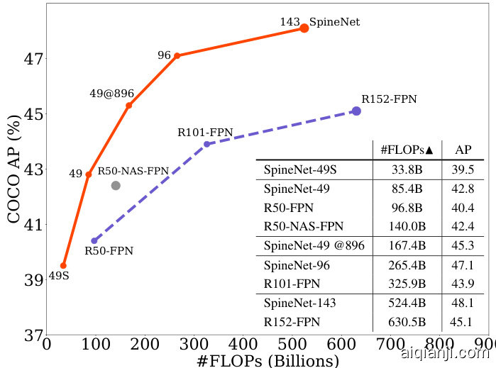
Figure 1: The comparison of RetinaNet models adopting SpineNet, ResNet-FPN, and NAS-FPN backbones. Details of training setup is described in Section 5 and controlled experiments can be found in Table 2, 3.
图 1: 采用 SpineNet、ResNet-FPN 和 NAS-FPN 骨干网络的 RetinaNet 模型对比。训练设置细节详见第 5 节,对照实验数据参见表 2 和表 3。

Figure 2: A comparison of mobile-size SpineNet models and other prior art of detectors for mobile-size object detection. Details are in Table 9.
图 2: 移动端尺寸SpineNet模型与其他移动端目标检测先进方法的对比。详细信息见表 9。
The scale-decreased model, however, may not be able to deliver strong features for multi-scale visual recognition tasks where recognition and localization are both important (e.g., object detection and segmentation). Lin et al. [21] shows directly using the top-level features from a scaledecreased model does not perform well on detecting small objects due to the low feature resolution. Several work including [21, 1] proposes multi-scale encoder-decoder architectures to address this issue. A scale-decreased network is taken as the encoder, which is commonly referred to a backbone model. Then a decoder network is applied to the backbone to recover the feature resolutions. The design of decoder network is drastically different from backbone model. A typical decoder network consists of a series of cross-scales connections that combine low-level and highlevel features from a backbone to generate strong multiscale feature maps. Typically, a backbone model has more parameters and computation (e.g., ResNets [10]) than a decoder model (e.g., feature pyramid networks [21]). Increasing the size of backbone model while keeping the decoder the same is a common strategy to obtain stronger encoderdecoder model.
然而,规模缩减模型可能无法为多尺度视觉识别任务(如目标检测和分割)提供强特征,这类任务中识别与定位都至关重要。Lin等人[21]指出,由于特征分辨率较低,直接使用规模缩减模型的顶层特征在小物体检测上表现不佳。[21, 1]等多项研究提出多尺度编码器-解码器架构以解决该问题:采用规模缩减网络作为编码器(通常称为骨干模型),再通过解码器网络恢复特征分辨率。解码器网络的设计与骨干模型存在显著差异——典型解码器由一系列跨尺度连接构成,通过融合骨干模型的低层与高层特征来生成强多尺度特征图。通常骨干模型(如ResNets[10])比解码器模型(如特征金字塔网络[21])具有更多参数和计算量。保持解码器不变的同时增大骨干模型规模,是获得更强编码器-解码器模型的常见策略。
In this paper, we aim to answer the question: Is the scaledecreased model a good backbone architecture design for simultaneous recognition and localization? Intuitively, a scale-decreased backbone throws away the spatial information by down-sampling, making it challenging to recover by a decoder network. In light of this, we propose a metaarchitecture, called scale-permuted model, with two major improvements on backbone architecture design. First, the scales of intermediate feature maps should be able to increase or decrease anytime so that the model can retain spatial information as it grows deeper. Second, the connections between feature maps should be able to go across feature scales to facilitate multi-scale feature fusion. Figure 3 demonstrates the differences between scale-decreased and scale-permuted networks.
本文旨在回答一个问题:尺度递减模型是否适合作为同步识别与定位的骨干网络架构?直观来看,通过下采样丢弃空间信息的尺度递减骨干网络,会为解码器网络的特征恢复带来挑战。为此,我们提出名为"尺度置换模型"的元架构,其骨干网络设计包含两大改进:首先,中间特征图的尺度应能动态增减,使模型在加深过程中保留空间信息;其次,特征图间的连接应能跨尺度交互以促进多尺度特征融合。图3展示了尺度递减网络与尺度置换网络的差异。
Although we have a simple meta-architecture design in mind, the possible instantiations grow combinatorial ly with the model depth. To avoid manually sifting through the tremendous amounts of design choices, we leverage Neural Architecture Search (NAS) [44] to learn the architecture. The backbone model is learned on the object detection task in COCO dataset [23], which requires simultaneous recognition and localization. Inspired by the recent success of NAS-FPN [6], we use the simple one-stage RetinaNet detector [22] in our experiments. In contrast to learning feature pyramid networks in NAS-FPN, we learn the backbone model architecture and directly connect it to the following classification and bounding box regression subnets. In other words, we remove the distinction between backbone and decoder models. The whole backbone model can be viewed and used as a feature pyramid network.
虽然我们心中有一个简单的元架构设计,但随着模型深度的增加,可能的实例化组合呈指数级增长。为了避免手动筛选海量的设计选择,我们利用神经架构搜索 (NAS) [44] 来学习架构。骨干模型是在 COCO 数据集 [23] 的目标检测任务上学习的,该任务需要同时进行识别和定位。受 NAS-FPN [6] 近期成功的启发,我们在实验中使用了简单的一阶段 RetinaNet 检测器 [22]。与 NAS-FPN 中学习特征金字塔网络不同,我们学习骨干模型架构并将其直接连接到后续的分类和边界框回归子网络。换句话说,我们消除了骨干模型和解码器模型之间的区别。整个骨干模型可以被视为并用作特征金字塔网络。

Figure 3: An example of scale-decreased network (left) vs. scalepermuted network (right). The width of block indicates feature resolution and the height indicates feature dimension. Dotted arrows represent connections from/to blocks not plotted.
图 3: 尺度缩减网络(左)与尺度置换网络(右)的对比示例。区块宽度表示特征分辨率,高度表示特征维度。虚线箭头代表未绘制的区块间连接。
Taking ResNet-50 [10] backbone as our baseline, we use the bottleneck blocks in ResNet-50 as the candidate feature blocks in our search space. We learn (1) the permutations of feature blocks and (2) the two input connections for each feature block. All candidate models in the search space have roughly the same computation as ResNet-50 since we just permute the ordering of feature blocks to obtain candidate models. The learned scale-permuted model outperforms ResNet-50-FPN by $(+2.9%A P)$ in the object detection task. The efficiency can be further improved (- $10%$ FLOPs) by adding search options to adjust scale and type (e.g., residual block or bottleneck block) of each candidate feature block. We name the learned scale-permuted backbone architecture SpineNet. Extensive experiments demonstrate that scale permutation and cross-scale connections are critical for building a strong backbone model for object detection. Figure 1 shows comprehensive comparisons of SpineNet to recent work in object detection.
以ResNet-50 [10]作为基线网络,我们将其中的瓶颈块(bottleneck block)作为搜索空间中的候选特征块。我们学习:(1) 特征块的排列组合 (2) 每个特征块的两条输入连接。由于仅通过重排特征块顺序生成候选模型,搜索空间中所有模型的计算量均与ResNet-50相近。在目标检测任务中,学习得到的尺度置换模型(scale-permuted model)性能超越ResNet-50-FPN达$(+2.9%AP)$。通过增加搜索选项来调整每个候选特征块的尺度和类型(例如残差块或瓶颈块),可进一步提升效率(减少$10%$FLOPs)。我们将学习得到的尺度置换主干架构命名为SpineNet。大量实验表明,尺度置换和跨尺度连接对于构建强大的目标检测主干模型至关重要。图1展示了SpineNet与近期目标检测工作的全面对比。
We further evaluate SpineNet on ImageNet and iNaturalist classification datasets. Even though SpineNet architec- ture is learned with object detection, it transfers well to classification tasks. Particularly, SpineNet outperforms ResNet by $5%$ top-1 accuracy on i Naturalist fine-grained classification dataset, where the classes need to be distinguished with subtle visual differences and localized features. The ability of directly applying SpineNet to classification tasks shows that the scale-permuted backbone is versatile and has the potential to become a unified model architecture for many visual recognition tasks.
我们进一步在ImageNet和iNaturalist分类数据集上评估SpineNet。尽管SpineNet架构是通过目标检测学习的,但它能很好地迁移到分类任务中。特别是,SpineNet在iNaturalist细粒度分类数据集上的top-1准确率比ResNet高出5%,该数据集的类别需要通过细微的视觉差异和局部特征进行区分。SpineNet能够直接应用于分类任务,表明这种尺度置换主干具有多功能性,并有可能成为多种视觉识别任务的统一模型架构。
2. Related Work
2. 相关工作
2.1. Backbone Model
2.1. 骨干模型 (Backbone Model)
The progress of developing convolutional neural networks has mainly been demonstrated on ImageNet classification dataset [4]. Researchers have been improving model by increasing network depth [18], novel network connections [10, 35, 36, 34, 14, 13], enhancing model capac- ity [43, 17] and efficiency [3, 32, 12, 38]. Several works have demonstrated that using a model with higher ImageNet accuracy as the backbone model achieves higher accuracy in other visual prediction tasks [16, 21, 1].
卷积神经网络的发展进程主要在ImageNet分类数据集[4]上得到验证。研究者们通过增加网络深度[18]、创新网络连接方式[10, 35, 36, 34, 14, 13]、提升模型容量[43, 17]以及优化效率[3, 32, 12, 38]来持续改进模型。多项研究表明,采用ImageNet准确率更高的模型作为骨干网络,能在其他视觉预测任务中获得更优性能[16, 21, 1]。

Figure 4: Building scale-permuted network by permuting ResNet. From (a) to (d), the computation gradually shifts from ResNet-FPN to scale-permuted networks. (a) The R50-FPN model, spending most computation in ResNet-50 followed by a FPN, achieves $37.8%$ AP; (b) R23-SP30, investing 7 blocks in a ResNet and 10 blocks in a scale-permuted network, achieves $39.6%$ AP; (c) R0-SP53, investing all blocks in a scale-permuted network, achieves $40.7%$ AP; (d) The SpineNet-49 architecture achieves $40.8%$ AP with $10%$ fewer FLOPs (85.4B vs. 95.2B) by learning additional block adjustments. Rectangle block represent bottleneck block and diamond block represent residual block. Output blocks are indicated by red border.
图 4: 通过重排ResNet构建尺度置换网络。从(a)到(d),计算过程逐渐从ResNet-FPN转向尺度置换网络。(a) R50-FPN模型将大部分计算集中在ResNet-50后接FPN,达到37.8% AP;(b) R23-SP30在ResNet中分配7个模块,在尺度置换网络中分配10个模块,达到39.6% AP;(c) R0-SP53将所有模块分配至尺度置换网络,达到40.7% AP;(d) SpineNet-49架构通过学习额外的模块调整,以减少10% FLOPs(85.4B vs. 95.2B)实现40.8% AP。矩形模块表示瓶颈模块,菱形模块表示残差模块。输出模块以红色边框标示。
However, the backbones developed for ImageNet may not be effective for localization tasks, even combined with a decoder network such as [21, 1]. DetNet [20] argues that down-sampling features compromises its localization capability. HRNet [40] attempts to address the problem by adding parallel multi-scale inter-connected branches. Stacked Hourglass [27] and FishNet [33] propose recurrent down-sample and up-sample architecture with skip connections. Unlike backbones developed for ImageNet, which are mostly scale-decreased, several works above have considered backbones built with both down-sample and up-sample operations. In Section 5.5 we compare the scale-permuted model with Hourglass and Fish shape architectures.
然而,为ImageNet设计的骨干网络即便搭配[21, 1]等解码器网络,在定位任务中也可能表现不佳。DetNet [20]指出下采样特征会损害定位能力。HRNet [40]通过添加并行多尺度互联分支试图解决该问题。Stacked Hourglass [27]和FishNet [33]提出了带跳跃连接的循环下采样-上采样架构。与主要为降尺度设计的ImageNet骨干网络不同,上述研究考虑了同时包含降采样和上采样操作的骨干网络。第5.5节我们将尺度置换模型与沙漏形、鱼形架构进行对比。
2.2. Neural Architecture Search
2.2. 神经架构搜索 (Neural Architecture Search)
Neural Architecture Search (NAS) has shown improvements over handcrafted models on image classification in the past few years [45, 25, 26, 41, 29, 38]. Unlike handcrafted networks, NAS learns architectures in the given search space by optimizing the specified rewards. Recent work has applied NAS for vision tasks beyond classification. NAS-FPN [6] and Auto-FPN [42] are pioneering works to apply NAS for object detection and focus on learning multi-layer feature pyramid networks. DetNAS [2] learns the backbone model and combines it with standard FPN [21]. Besides object detection, Auto-DeepLab [24] learns the backbone model and combines it with decoder in DeepLabV3 [1] for semantic segmentation. All aforementioned works except Auto-DeepLab learn or use a scaledecreased backbone model for visual recognition.
神经架构搜索 (Neural Architecture Search, NAS) 在过去几年中已证明其在图像分类任务上优于手工设计模型 [45, 25, 26, 41, 29, 38]。与人工设计的网络不同,NAS 通过优化指定奖励在给定搜索空间中学习架构。近期研究已将 NAS 应用于分类之外的视觉任务:NAS-FPN [6] 和 Auto-FPN [42] 是将 NAS 应用于目标检测的开创性工作,专注于学习多层特征金字塔网络;DetNAS [2] 学习主干模型并与标准 FPN [21] 结合;除目标检测外,Auto-DeepLab [24] 学习主干模型并与 DeepLabV3 [1] 的解码器结合用于语义分割。除 Auto-DeepLab 外,上述所有工作都学习或使用尺度缩减的主干模型进行视觉识别。
3. Method
3. 方法
The architecture of the proposed backbone model consists of a fixed stem network followed by a learned scalepermuted network. A stem network is designed with scaledecreased architecture. Blocks in the stem network can be candidate inputs for the following scale-permuted network.
所提出的骨干模型架构由一个固定的主干网络和一个可学习的尺度置换网络组成。主干网络采用尺度递减架构设计,其中的模块可作为后续尺度置换网络的候选输入。
A scale-permuted network is built with a list of building blocks ${{\bf B}_ {1},{\bf B}_ {2},\cdot\cdot\cdot,{\bf B}_ {N}}$ . Each block $\mathbf{B}_ {k}$ has an associated feature level $L_ {i}$ . Feature maps in an $L_ {i}$ block have a resolution of $\frac{1}{2^{i}}$ of the input resolution. The blocks in the same level have an identical architecture. Inspired by NASFPN [6], we define 5 output blocks from $L_ {3}$ to $L_ {7}$ and a $1\times1$ convolution attached to each output block to produce multi-scale features $P_ {3}$ to $P_ {7}$ with the same feature dimension. The rest of the building blocks are used as intermediate blocks before the output blocks. In Neural Architecture Search, we first search for scale permutations for the intermediate and output blocks then determine cross-scale connections between blocks. We further improve the model by adding block adjustments in the search space.
尺度置换网络由一系列构建块 ${{\bf B}_ {1},{\bf B}_ {2},\cdot\cdot\cdot,{\bf B}_ {N}}$ 组成。每个块 $\mathbf{B}_ {k}$ 关联一个特征层级 $L_ {i}$ ,其中 $L_ {i}$ 级块的特征图分辨率为输入分辨率的 $\frac{1}{2^{i}}$ 。同级块采用相同架构。受NASFPN [6] 启发,我们定义了从 $L_ {3}$ 到 $L_ {7}$ 的5个输出块,并为每个输出块附加 $1\times1$ 卷积以生成具有相同特征维度的多尺度特征 $P_ {3}$ 至 $P_ {7}$ ,其余构建块作为输出块前的中间块。在神经架构搜索中,我们首先搜索中间块与输出块的尺度排列组合,进而确定块间的跨尺度连接。通过向搜索空间加入块调整机制,我们进一步改进了模型。
3.1. Search Space
3.1. 搜索空间
Scale permutations: The orderings of blocks are important because a block can only connect to its parent blocks which have lower orderings. We define the search space of scale permutations by permuting intermediate and output blocks respectively, resulting in a search space size of $(N-5)!5!$ . The scale permutations are first determined before searching for the rest of the architecture.
规模排列:块的顺序至关重要,因为每个块只能连接到排序更低的父块。我们通过分别置换中间块和输出块来定义规模排列的搜索空间,其空间大小为$(N-5)!5!$。在搜索架构其余部分前,需优先确定规模排列方案。
Cross-scale connections: We define two input connections for each block in the search space. The parent blocks can be any block with a lower ordering or block from the stem network. Resampling spatial and feature dimensions is needed when connecting blocks in different feature levels. The search space has a size of $\textstyle\prod_ {i=m}^{N+m-1}C_ {2}^{i}$ , where $m$ is the number of candidate blocks i n the stem network.
跨尺度连接:我们为搜索空间中的每个块定义了两个输入连接。父块可以是任何序号较低的块或来自主干网络的块。当连接不同特征层级的块时,需要重采样空间和特征维度。该搜索空间的大小为$\textstyle\prod_ {i=m}^{N+m-1}C_ {2}^{i}$,其中$m$表示主干网络中的候选块数量。
Block adjustments: We allow block to adjust its scale level and type. The intermediate blocks can adjust levels by ${-1,0,1,2}$ , resulting in a search space size of $4^{N-5}$ . All blocks are allowed to select one between the two options {bottleneck block, residual block} described in [10], resulting in a search space size of $2^{N}$ .
块调整:我们允许块调整其尺度级别和类型。中间块可以通过 ${-1,0,1,2}$ 调整级别,从而产生 $4^{N-5}$ 的搜索空间大小。所有块都可以在[10]中描述的两种选项{瓶颈块(bottleneck block)、残差块(residual block)}之间选择一种,从而产生 $2^{N}$ 的搜索空间大小。
3.2. Resampling in Cross-scale Connections
3.2. 跨尺度连接中的重采样
One challenge in cross-scale feature fusion is that the resolution and feature dimension may be different among parent and target blocks. In such case, we perform spatial and feature resampling to match the resolution and feature dimension to the target block, as shown in detail in Figure 5. Here, $C$ is the feature dimension of $3\times3$ convolution in residual or bottleneck block. We use $C^{i n}$ and $C^{o u t}$ to indicate the input and output dimension of a block. For bottleneck block, $C^{i n}=C^{o u t}=4C$ ; and for residual block, Cin = Cout = C. As it is important to keep the computational cost in resampling low, we introduce a scaling factor $\alpha$ (default value 0.5) to adjust the output feature dimension $C^{o u t}$ in a parent block to $\alpha C$ . Then, we use a nearest-neighbor interpolation for up-sampling or a stride $23\times3$ convolution (followed by stride-2 max poolings if necessary) for down-sampling feature map to match to the target resolution. Finally, a $1\times1$ convolution is applied to match feature dimension $\alpha C$ to the target feature dimension $C^{i n}$ . Following FPN [21], we merge the two resampled input feature maps with elemental-wise addition.
跨尺度特征融合的一个挑战在于,父块与目标块之间的分辨率和特征维度可能不同。针对这种情况,我们会执行空间和特征重采样来匹配目标块的分辨率与特征维度,具体如图 5 所示。其中,$C$ 表示残差块或瓶颈块中 $3\times3$ 卷积的特征维度。我们用 $C^{in}$ 和 $C^{out}$ 分别表示块的输入和输出维度。对于瓶颈块,$C^{in}=C^{out}=4C$;对于残差块,$C^{in}=C^{out}=C$。为保持重采样的计算成本处于较低水平,我们引入缩放因子 $\alpha$(默认值 0.5)将父块的输出特征维度 $C^{out}$ 调整为 $\alpha C$。随后采用最近邻插值进行上采样,或使用步长为 2 的 $3\times3$ 卷积(必要时接步长为 2 的最大池化)进行下采样,以匹配目标分辨率。最后通过 $1\times1$ 卷积将特征维度 $\alpha C$ 调整至目标特征维度 $C^{in}$。遵循 FPN [21] 的方法,我们对两个重采样后的输入特征图进行逐元素相加融合。
3.3. Scale-Permuted Model by Permuting ResNet
3.3. 通过置换 ResNet 构建的尺度重排模型
Here we build scale-permuted models by permuting feature blocks in ResNet architecture. The idea is to have a fair comparison between scale-permuted model and scaledecreased model when using the same building blocks. We make small adaptation for scale-permuted models to generate multi-scale outputs by replacing one $L_ {5}$ block in
在此我们通过重新排列ResNet架构中的特征块来构建尺度置换模型。这一设计旨在使用相同构建块时,能对尺度置换模型和尺度递减模型进行公平比较。我们对尺度置换模型做了微小调整,通过替换一个$L_ {5}$块来生成多尺度输出。

Figure 5: Resampling operations. Spatial resampling to upsample (top) and to downsample (bottom) input features followed by resampling in feature dimension before feature fusion. Table 1: Number of blocks per level for stem and scalepermuted networks. The scale-permuted network is built on top of a scale-decreased stem network as shown in Figure 4. The size of scale-decreased stem network is gradually decreased to show the effectiveness of scale-permuted network.
| stemnetwork {L2,L3,L4,L5} | scale-permuted network {L2,L3,L4,L5,L6,L7} | |
| R50 | {3,4,6,3} | {-} |
| R35-SP18 R23-SP30 | {2,3,5,1} | {1, 1, 1, 1, 1, 1} |
| R14-SP39 | {2,2,2,1} {1,1,1,1} | {1,2,4,1,1,1} |
| RO-SP53 | {2,3,5,1,1,1} | |
| SpineNet-49 | {2,0,0,0} {2,0,0,0} | {1,4,6,2,1,1} {1,2,4,4,2,2} |
图 5: 重采样操作。空间重采样用于上采样(顶部)和下采样(底部)输入特征,随后在特征融合前进行特征维度的重采样。
表 1: 主干网络和尺度置换网络各层级块数。尺度置换网络构建在如图4所示的尺度递减主干网络之上。尺度递减主干网络的尺寸逐渐减小以展示尺度置换网络的有效性。
| 主干网络 {L2,L3,L4,L5} | 尺度置换网络 {L2,L3,L4,L5,L6,L7} | |
|---|---|---|
| R50 | {3,4,6,3} | {-} |
| R35-SP18 R23-SP30 | {2,3,5,1} | {1, 1, 1, 1, 1, 1} |
| R14-SP39 | {2,2,2,1} {1,1,1,1} | {1,2,4,1,1,1} |
| RO-SP53 | {2,3,5,1,1,1} | |
| SpineNet-49 | {2,0,0,0} {2,0,0,0} | {1,4,6,2,1,1} {1,2,4,4,2,2} |
ResNet with one $L_ {6}$ and one $L_ {7}$ blocks and set the feature dimension to 256 for $L_ {5}$ , $L_ {6}$ , and $L_ {7}$ blocks. In addition to comparing fully scale-decreased and scale-permuted model, we create a family of models that gradually shifts the model from the scale-decreased stem network to the scalepermuted network. Table 1 shows an overview of block allocation of models in the family. We use $\mathsf{R}[N]\mathrm{-SP}[M]$ to indicate $N$ feature layers in the handcrafted stem network and $M$ feature layers in the learned scale-permuted network.
带有1个$L_ {6}$和1个$L_ {7}$块的ResNet,并将$L_ {5}$、$L_ {6}$和$L_ {7}$块的特征维度设置为256。除了比较完全尺度递减和尺度置换模型外,我们还创建了一系列逐步从尺度递减主干网络过渡到尺度置换网络的模型。表1展示了该系列模型中块分配的概览。我们使用$\mathsf{R}[N]\mathrm{-SP}[M]$表示手工设计主干网络中的$N$个特征层和学习尺度置换网络中的$M$个特征层。
For a fair comparison, we constrain the search space to only include scale permutations and cross-scale connections. Then we use reinforcement learning to train a controller to generate model architectures. similar to [6], for intermediate blocks that do not connect to any block with a higher ordering in the generated architecture, we connect them to the output block at the corresponding level. Note that the cross-scale connections only introduce small computation overhead, as discussed in Section 3.2. As a result, all models in the family have similar computation as ResNet-50. Figure 4 shows a selection of learned model architectures in the family.
为了公平比较,我们将搜索空间限制为仅包含尺度排列和跨尺度连接。随后采用强化学习训练控制器来生成模型架构。与[6]类似,对于生成架构中未连接更高序号块的中间块,我们会将其连接到对应层级的输出块。需注意的是,如第3.2节所述,跨尺度连接仅引入微小计算开销。因此,该系列所有模型的计算量与ResNet-50相近。图4展示了该系列中部分习得的模型架构。
3.4. SpineNet Architectures
3.4. SpineNet架构
To this end, we design scale-permuted models with a fair comparison to ResNet. However, using ResNet-50 building blocks may not be an optimal choice for building scalepermuted models. We suspect the optimal model may have different feature resolution and block type distributions than
为此,我们设计了与ResNet公平对比的尺度置换模型。但使用ResNet-50构建块可能不是构建尺度置换模型的最佳选择。我们推测最优模型可能具有不同的特征分辨率和块类型分布。

Figure 6: Increase model depth by block repeat. From left to right: blocks in SpineNet-49, SpineNet-96, and SpineNet-143.
图 6: 通过块重复增加模型深度。从左到右分别为: SpineNet-49、SpineNet-96 和 SpineNet-143 中的块结构。
ResNet. Therefore, we further include additional block adjustments in the search space as proposed in Section 3.1. The learned model architecture is named SpineNet-49, of which the architecture is shown in Figure 4d and the number of blocks per level is given in Table 1.
ResNet。因此,我们进一步在搜索空间中纳入了第3.1节提出的额外块调整。学习到的模型架构命名为SpineNet-49,其架构如图4d所示,各层级块数量见表1。
Based on SpineNet-49, we construct four architectures in the SpineNet family where the models perform well for a wide range of latency-performance trade-offs. The models are denoted as SpineNet-49S/96/143/190: SpineNet-49S has the same architecture as SpineNet-49 but the feature dimensions in the entire network are scaled down uniformly by a factor of 0.65. SpineNet-96 doubles the model size by repeating each block $\mathbf{B}_ {k}$ twice. The building block $\mathbf{B}_ {k}$ is duplicated into $\mathbf{B}_ {k}^{1}$ and $\mathbf{B}_ {k}^{2}$ , which are then sequentially connected. The first block $\mathbf{B}_ {k}^{1}$ connects to input parent blocks and the last block $\mathbf{B}_ {k}^{2}$ connects to output target blocks. SpineNet-143 and SpineNet-190 repeat each block 3 and 4 times to grow the model depth and adjust $\alpha$ in the resampling operation to 1.0. SpineNet-190 further scales up feature dimension uniformly by 1.3. Figure 6 shows an example of increasing model depth by repeating blocks.
基于SpineNet-49,我们构建了SpineNet家族的四种架构,这些模型在广泛的延迟-性能权衡范围内表现良好。这些模型分别命名为SpineNet-49S/96/143/190:
- SpineNet-49S架构与SpineNet-49相同,但整个网络中的特征维度统一缩小了0.65倍。
- SpineNet-96通过将每个块$\mathbf{B}_ {k}$重复两次来使模型规模翻倍。构建块$\mathbf{B}_ {k}$被复制为$\mathbf{B}_ {k}^{1}$和$\mathbf{B}_ {k}^{2}$,然后依次连接。第一个块$\mathbf{B}_ {k}^{1}$连接到输入父块,最后一个块$\mathbf{B}_ {k}^{2}$连接到输出目标块。
- SpineNet-143和SpineNet-190分别将每个块重复3次和4次以增加模型深度,并将重采样操作中的$\alpha$调整为1.0。SpineNet-190还进一步将特征维度统一扩大了1.3倍。
图6展示了通过重复块来增加模型深度的示例。
Note we do not apply recent work on new building blocks (e.g., Shuffle Ne tv 2 block used in DetNas [2]) or efficient model scaling [38] to SpineNet. These improvements could be orthogonal to this work.
需要注意的是,我们没有将近期关于新构建模块(如DetNas [2]中使用的Shuffle Net v2模块)或高效模型扩展 [38] 的研究应用于SpineNet。这些改进可能与本研究正交。
4. Applications
4. 应用
4.1. Object Detection
4.1. 目标检测
The SpineNet architecture is learned with RetinaNet detector by simply replacing the default ResNet-FPN backbone model. To employ SpineNet in RetinaNet, we follow the architecture design for the class and box subnets in [22]: For SpineNet-49S, we use 4 shared convolutional layers at feature dimension 128; For SpineNet-49/96/143, we use 4 shared convolutional layers at feature dimension 256; For SpineNet-190, we scale up subnets by using 7 shared convolutional layers at feature dimension 512. To employ SpineNet in Mask R-CNN, we follow the same architecture design in [8]: For SpineNet-49S/49/96/143, we use 1 shared convolutional layers at feature dimension 256 for RPN, 4 shared convolutional layers at feature dimension
SpineNet架构通过简单替换默认的ResNet-FPN主干模型,与RetinaNet检测器共同学习。在RetinaNet中使用SpineNet时,我们遵循[22]中分类与边界框子网络的设计方案:对于SpineNet-49S,采用特征维度128的4层共享卷积;对于SpineNet-49/96/143,采用特征维度256的4层共享卷积;对于SpineNet-190,通过特征维度512的7层共享卷积实现子网络扩展。在Mask R-CNN中应用SpineNet时,沿用[8]的相同架构设计:对于SpineNet-49S/49/96/143,RPN模块使用特征维度256的1层共享卷积,分类与边界框子网络采用特征维度256的4层共享卷积。
256 followed by a fully-connected layers of 1024 units for detection branch, and 4 shared convolutional layers at feature dimension 256 for mask branch. For SpineNet-49S, we use 128 feature dimension for convolutional layers in subnets. For SpineNet-190, we scale up detection subnets by using 7 convolutional layers at feature dimension 384.
256,随后检测分支采用1024个单元的全连接层,掩码分支采用4个特征维度为256的共享卷积层。对于SpineNet-49S,我们在子网络中使用128特征维度的卷积层。对于SpineNet-190,我们通过使用7个特征维度为384的卷积层来扩展检测子网络。
4.2. Image Classification
4.2. 图像分类
To demonstrate SpineNet has the potential to generalize to other visual recognition tasks, we apply SpineNet to image classification. We utilize the same $P_ {3}$ to $P_ {7}$ feature pyramid to construct the classification network. Specifically, the final feature map $\begin{array}{r}{P=\frac{1}{5}\sum_ {i=3}^{7}\mathcal{U}(P_ {i})}\end{array}$ is generated by upsampling and averaging the feature maps, where $\mathcal{U}(\cdot)$ is the nearest-neighbor upsampling to ensure all feature maps have the same scale as the largest feature map $P_ {3}$ . The standard global average pooling on $P$ is applied to produce a 256-dimensional feature vector followed by a linear classifier with softmax for classification.
为验证SpineNet在其他视觉识别任务中的泛化能力,我们将其应用于图像分类任务。采用相同的 $P_ {3}$ 至 $P_ {7}$ 特征金字塔构建分类网络。具体而言,最终特征图 $\begin{array}{r}{P=\frac{1}{5}\sum_ {i=3}^{7}\mathcal{U}(P_ {i})}\end{array}$ 通过对各层级特征图进行上采样和均值计算生成,其中 $\mathcal{U}(\cdot)$ 采用最近邻上采样以确保所有特征图与最大尺度特征图 $P_ {3}$ 保持相同分辨率。对 $P$ 执行标准全局平均池化后,生成256维特征向量并输入带softmax的线性分类器完成分类。
5. Experiments
5. 实验
For object detection, we evaluate SpineNet on COCO dataset [23]. All the models are trained on the train2017 split. We report our main results with COCO AP on the test-dev split and others on the val2017 split. For image classification, we train SpineNet on ImageNet ILSVRC-2012 [31] and i Naturalist-2017 [39] and report Top-1 and Top-5 validation accuracy.
在目标检测任务中,我们在COCO数据集[23]上评估SpineNet。所有模型均在train2017子集上训练,主要结果以test-dev子集的COCO AP指标呈现,其余结果基于val2017子集。对于图像分类任务,我们在ImageNet ILSVRC-2012[31]和iNaturalist-2017[39]上训练SpineNet,并报告Top-1和Top-5验证准确率。
5.1. Experimental Settings
5.1. 实验设置
Training data pre-processing: For object detection, we feed a larger image, from 640 to 896, 1024, 1280, to a larger SpineNet. The long side of an image is resized to the target size then the short side is padded with zeros to make a square image. For image classification, we use the standard input size of $224\times224$ . During training, we adopt standard data augmentation (scale and aspect ratio augmentation, random cropping and horizontal flipping).
训练数据预处理:对于目标检测任务,我们向更大的SpineNet输入尺寸从640到896、1024、1280不等的图像。图像的长边会被调整至目标尺寸,短边则用零填充以形成正方形图像。在图像分类任务中,我们采用标准输入尺寸$224\times224$。训练过程中,我们应用了标准数据增强方法(包括缩放与长宽比调整、随机裁剪以及水平翻转)。
Training details: For object detection, we generally follow [22, 6] to adopt the same training protocol, denoting as protocol A, to train SpineNet and ResNet-FPN models for controlled experiments described in Figure 4. In brief, we use stochastic gradient descent to train on Cloud TPU v3 devices with 4e-5 weight decay and 0.9 momentum. All models are trained from scratch on COCO train2017 with 256 batch size for 250 epochs. The initial learning rate is set to 0.28 and a linear warmup is applied in the first 5 epochs. We apply stepwise learning rate that decays to $0.1\times$ and $0.01\times$ at the last 30 and 10 epoch. We follow [8] to apply synchronized batch normalization with 0.99 momentum followed by ReLU and implement DropBlock [5] for regu lari z ation. We apply multi-scale training with a random scale between [0.8, 1.2] as in [6]. We set base anchor size to 3 for SpineNet-96 or smaller models and 4 for SpineNet143 or larger models in RetinaNet implementation. For our reported results, we adopt an improved training protocol denoting as protocol B. For simplicity, protocol B removes DropBlock and apply stronger multi-scale training with a random scale between [0.5, 2.0] for 350 epochs. To obtain the most competitive results, we add stochastic depth with keep prob 0.8 [15] for stronger regular iz ation and replace ReLU with swish activation [28] to train all models for 500 epochs, denoting as protocol C. We also adopt a more aggressive multi-scale training strategy with a random scale between [0.1, 2.0] for SpineNet-143/190 when using protocol C. For image classification, all models are trained with a batch size of 4096 for 200 epochs. We used cosine learning rate decay [11] with linear scaling of learning rate and gradual warmup in the first 5 epochs [7].
训练细节:
对于目标检测任务,我们基本遵循[22, 6]采用相同的训练方案(记为方案A)来训练SpineNet和ResNet-FPN模型,以进行图4所述的对照实验。简而言之,我们使用随机梯度下降在Cloud TPU v3设备上进行训练,权重衰减为4e-5,动量为0.9。所有模型均在COCO train2017数据集上从头开始训练,批量大小为256,共训练250个周期。初始学习率设为0.28,并在前5个周期采用线性预热。我们采用阶梯式学习率调度,在最后30个和10个周期时分别衰减至$0.1\times$和$0.01\times$。参照[8],我们使用动量为0.99的同步批量归一化,后接ReLU激活函数,并采用DropBlock[5]进行正则化。按照[6]的方法,我们实施多尺度训练,随机缩放比例范围为[0.8, 1.2]。在RetinaNet实现中,对于SpineNet-96或更小的模型,我们将基础锚框大小设为3;对于SpineNet-143或更大的模型则设为4。
报告结果时,我们采用了改进的训练方案(记为方案B)。简而言之,方案B移除了DropBlock,并采用更强的多尺度训练(随机缩放比例范围为[0.5, 2.0])进行350个周期的训练。为获得最具竞争力的结果,我们进一步添加了保持概率为0.8的随机深度[15]以增强正则化,并将ReLU替换为swish激活函数[28],训练所有模型500个周期(记为方案C)。在使用方案C时,对于SpineNet-143/190模型,我们还采用了更激进的多尺度训练策略(随机缩放比例范围为[0.1, 2.0])。
对于图像分类任务,所有模型均以4096的批量大小训练200个周期。我们采用余弦学习率衰减[11],并在前5个周期[7]内进行学习率线性缩放和渐进式预热。
Table 2: One-stage object detection results on COCO test-dev. We compare employing different backbones with RetinaNet on single model without test-time augmentation. By default we apply protocol B with multi-scale training and ReLU activation to train all models in this table, as described in Section 5.1. Models marked by dagger $(^{\dagger})$ are trained with protocol C by applying stochastic depth and swish activation for a longer training schedule. FLOPs is represented by Multi-Adds.
| backbone model | resolution | #FLOPs | #Params | AP | AP50 | AP75 | APs | APM | APL |
| SpineNet-49S | 640×640 | 33.8B | 11.9M | 39.5 | 59.3 | 43.1 | 20.9 | 42.2 | 54.3 |
| SpineNet-49 | 640×640 | 85.4B | 28.5M | 42.8 | 62.3 | 46.1 | 23.7 | 45.2 | 57.3 |
| R50-FPN | 640×640 | 96.8B | 34.0M | 40.4 | 59.9 | 43.6 | 22.7 | 43.5 | 57.0 |
| R50-NAS-FPN | 640×640 | 140.0B | 60.3M | 42.4 | 61.8 | 46.1 | 25.1 | 46.7 | 57.8 |
| SpineNet-49 | 896×896 | 167.4B | 28.5M | 45.3 | 65.1 | 49.1 | 27.0 | 47.9 | 57.7 |
| SpineNet-96 | 1024×1024 | 265.4B | 43.0M | 47.1 | 67.1 | 51.1 | 29.1 | 50.2 | 59.0 |
| R101-FPN | 1024×1024 | 325.9B | 53.1M | 43.9 | 63.6 | 47.6 | 26.8 | 47.6 | 57.0 |
| SpineNet-143 | 1280×1280 | 524.4B | 66.9M | 48.1 | 67.6 | 52.0 | 30.2 | 51.1 | 59.9 |
| R152-FPN | 1280×1280 | 630.5B | 68.7M | 45.1 | 64.6 | 48.7 | 28.4 | 48.8 | 58.2 |
| R50-FPNt | 640×640 | 96.8B | 34.0M | 42.3 | 61.9 | 45.9 | 23.9 | 46.1 | 58.5 |
| SpineNet-49st | 640×640 | 33.8B | 12.0M | 41.5 | 60.5 | 44.6 | 23.3 | 45.0 | 58.0 |
| SpineNet-49t | 640×640 | 85.4B | 28.5M | 44.3 | 63.8 | 47.6 | 25.9 | 47.7 | 61.1 |
| SpineNet-49t | 896×896 | 167.4B | 28.5M | 46.7 | 66.3 | 50.6 | 29.1 | 50.1 | 61.7 |
| SpineNet-96t | 1024×1024 | 265.4B | 43.0M | 48.6 | 68.4 | 52.5 | 32.0 | 52.3 | 62.0 |
| SpineNet-143t | 1280×1280 | 524.4B | 66.9M | 50.7 | 70.4 | 54.9 | 33.6 | 53.9 | 62.1 |
| SpineNet-190t | 1280×1280 | 1885.0B | 163.6M | 52.1 | 71.8 | 56.5 | 35.4 | 55.0 | 63.6 |
表 2: COCO test-dev 数据集上的单阶段目标检测结果。我们比较了在单一模型上使用不同主干网络与 RetinaNet 的效果(未使用测试时增强)。默认情况下,本表所有模型均采用 5.1 节所述的协议 B 进行训练(包含多尺度训练和 ReLU 激活)。标有剑号 $(^{\dagger})$ 的模型采用协议 C 训练(应用随机深度和 swish 激活,并延长训练周期)。FLOPs 以 Multi-Adds 表示。
| 主干模型 | 分辨率 | FLOPs | 参数量 | AP | AP50 | AP75 | APs | APM | APL |
|---|---|---|---|---|---|---|---|---|---|
| SpineNet-49S | 640×640 | 33.8B | 11.9M | 39.5 | 59.3 | 43.1 | 20.9 | 42.2 | 54.3 |
| SpineNet-49 | 640×640 | 85.4B | 28.5M | 42.8 | 62.3 | 46.1 | 23.7 | 45.2 | 57.3 |
| R50-FPN | 640×640 | 96.8B | 34.0M | 40.4 | 59.9 | 43.6 | 22.7 | 43.5 | 57.0 |
| R50-NAS-FPN | 640×640 | 140.0B | 60.3M | 42.4 | 61.8 | 46.1 | 25.1 | 46.7 | 57.8 |
| SpineNet-49 | 896×896 | 167.4B | 28.5M | 45.3 | 65.1 | 49.1 | 27.0 | 47.9 | 57.7 |
| SpineNet-96 | 1024×1024 | 265.4B | 43.0M | 47.1 | 67.1 | 51.1 | 29.1 | 50.2 | 59.0 |
| R101-FPN | 1024×1024 | 325.9B | 53.1M | 43.9 | 63.6 | 47.6 | 26.8 | 47.6 | 57.0 |
| SpineNet-143 | 1280×1280 | 524.4B | 66.9M | 48.1 | 67.6 | 52.0 | 30.2 | 51.1 | 59.9 |
| R152-FPN | 1280×1280 | 630.5B | 68.7M | 45.1 | 64.6 | 48.7 | 28.4 | 48.8 | 58.2 |
| R50-FPNt | 640×640 | 96.8B | 34.0M | 42.3 | 61.9 | 45.9 | 23.9 | 46.1 | 58.5 |
| SpineNet-49st | 640×640 | 33.8B | 12.0M | 41.5 | 60.5 | 44.6 | 23.3 | 45.0 | 58.0 |
| SpineNet-49t | 640×640 | 85.4B | 28.5M | 44.3 | 63.8 | 47.6 | 25.9 | 47.7 | 61.1 |
| SpineNet-49t | 896×896 | 167.4B | 28.5M | 46.7 | 66.3 | 50.6 | 29.1 | 50.1 | 61.7 |
| SpineNet-96t | 1024×1024 | 265.4B | 43.0M | 48.6 | 68.4 | 52.5 | 32.0 | 52.3 | 62.0 |
| SpineNet-143t | 1280×1280 | 524.4B | 66.9M | 50.7 | 70.4 | 54.9 | 33.6 | 53.9 | 62.1 |
| SpineNet-190t | 1280×1280 | 1885.0B | 163.6M | 52.1 | 71.8 | 56.5 | 35.4 | 55.0 | 63.6 |
Table 3: Results comparisons between R50-FPN and scalepermuted models on COCO $\mathtt{v a l}2017$ by adopting protocol A. The performance improves with more computation being allocated to scale-permuted network. We also show the efficiency improvement by having scale and block type adjustments in Section 3.1.
| model | block adju. | #FLOPS | AP |
| R50-FPN | 96.8B | 37.8 | |
| R35-SP18 | 91.7B | 38.7 | |
| R23-SP30 | 96.5B | 39.7 | |
| R14-SP39 | 99.7B | 39.6 | |
| RO-SP53 | 95.2B | 40.7 | |
| SpineNet-49 | 85.4B | 40.8 |
表 3: 采用协议A时,R50-FPN与尺度置换(scale-permuted)模型在COCO $\mathtt{v a l}2017$数据集上的结果对比。随着更多计算资源分配给尺度置换网络,性能得到提升。第3.1节还展示了通过调整尺度和块类型带来的效率改进。
| 模型 | 块调整 | 浮点运算次数 | AP |
|---|---|---|---|
| R50-FPN | 96.8B | 37.8 | |
| R35-SP18 | 91.7B | 38.7 | |
| R23-SP30 | 96.5B | 39.7 | |
| R14-SP39 | 99.7B | 39.6 | |
| RO-SP53 | 95.2B | 40.7 | |
| SpineNet-49 | 85.4B | 40.8 |
Table 4: Inference latency of RetinaNet with SpineNet on a V100 GPU with NVIDIA TensorRT. Latency is measured for an end-toend object detection pipeline including pre-processing, detection generation, and post-processing (e.g., NMS).
| model | resolution | AP | inference latency |
| SpineNet-49S | 640×640 | 39.9 | 11.7ms |
| SpineNet-49 | 640×640 | 42.8 | 15.3ms |
| SpineNet-49 | 896×896 | 45.3 | 34.3ms |
表 4: 使用NVIDIA TensorRT在V100 GPU上运行RetinaNet与SpineNet的推理延迟。延迟测量包含端到端目标检测流程,包括预处理、检测生成和后处理(如NMS)。
| model | resolution | AP | inference latency |
|---|---|---|---|
| SpineNet-49S | 640×640 | 39.9 | 11.7ms |
| SpineNet-49 | 640×640 | 42.8 | 15.3ms |
| SpineNet-49 | 896×896 | 45.3 | 34.3ms |
NAS details: We implement the recurrent neural network based controller proposed in [44] for architecture search, as it is the only method we are aware of that supports searching for permutations. We reserve 7392 images from train2017 as the validation set for searching. To speed up the searching process, we design a proxy SpineNet by uniformly scaling down the feature dimension of SpineNet49 with a factor of 0.25, setting $\alpha$ in resampling to 0.25, and using feature dimension 64 in the box and class nets. To prevent the search space from growing exponentially, we restrict intermediate blocks to search for parent blocks within the last 5 blocks built and allow output blocks to search from all existing blocks. At each sample, a proxy task is trained at image resolution 512 for 5 epochs. AP of the proxy task on the reserved validation set is collected as reward. The controller uses 100 Cloud TPU v3 in parallel to sample child models. The best architectures for R35-SP18, R23-SP30, R14-SP39, R0-SP53, and SpineNet-49 are found after 6k, 10k, 13k, $13\mathrm{k\Omega}$ , and $14\mathrm{k\Omega}$ architectures are sampled.
NAS细节:我们采用[44]中提出的基于循环神经网络的控制器进行架构搜索,因为这是目前已知唯一支持搜索排列组合的方法。我们从train2017数据集中保留7392张图像作为搜索验证集。为加速搜索过程,设计了代理版SpineNet:将SpineNet49的特征维度统一缩放0.25倍,重采样参数α设为0.25,并在边界框和分类网络中使用64维特征。为防止搜索空间指数级增长,限制中间模块只能从最近构建的5个模块中选择父模块,同时允许输出模块从所有现有模块中搜索。每次采样时,代理任务以512分辨率图像训练5个周期,其在保留验证集上的AP指标作为奖励信号。控制器使用100个Cloud TPU v3并行采样子模型。R35-SP18、R23-SP30、R14-SP39、R0-SP53和SpineNet-49的最佳架构分别在采样6k、10k、13k、13kΩ和14kΩ个架构后确定。
Table 5: Two-stage object detection and instance segmentation results. We compare employing different backbones with Mask R-CNN using 1000 proposals on single model without test-time augmentation. By default we apply protocol B with multi-scale training and ReLU activation to train all models in this table, as described in Section 5.1. SpineNet-190 (marked by †) is trained with protocol C by applying stochastic depth and swish activation for a longer training schedule. FLOPs is represented by Multi-Adds.
| backbone model | resolution | #FLOPs | #Params | APval | APmak | APtest-dev | |
| SpineNet-49S | 640×640 | 60.2B | 13.9M | 39.3 | 34.8 | - | |
| SpineNet-49 | 640×640 | 216.1B | 40.8M | 42.9 | 38.1 | ||
| R50-FPN | 640×640 | 227.7B | 46.3M | 42.7 | 37.8 | ||
| SpineNet-96 | 1024×1024 | 315.0B | 55.2M | 47.2 | 41.5 | ||
| R101-FPN | 1024×1024 | 375.5B | 65.3M | 46.6 | 41.2 | 二 | |
| SpineNet-143 | 1280×1280 | 498.8B | 79.2M | 48.8 | 42.7 | ||
| R152-FPN | 1280×1280 | 605.3B | 80.9M | 48.1 | 42.4 | - | |
| SpineNet-190 | 1536×1536 | 2076.8B | 176.2M | 52.2 | 46.1 | 52.5 | 46.3 |
表 5: 两阶段目标检测与实例分割结果对比。我们采用不同骨干网络与 Mask R-CNN (使用1000个候选框)在单模型无测试时增强的情况下进行对比。默认采用协议B (多尺度训练和ReLU激活)训练本表所有模型,如第5.1节所述。带†标记的SpineNet-190采用协议C训练 (应用随机深度和swish激活函数,延长训练周期)。FLOPs以Multi-Adds表示。
| 骨干模型 | 分辨率 | FLOPs | 参数量 | APval | APmak | APtest-dev | |
|---|---|---|---|---|---|---|---|
| SpineNet-49S | 640×640 | 60.2B | 13.9M | 39.3 | 34.8 | - | |
| SpineNet-49 | 640×640 | 216.1B | 40.8M | 42.9 | 38.1 | ||
| R50-FPN | 640×640 | 227.7B | 46.3M | 42.7 | 37.8 | ||
| SpineNet-96 | 1024×1024 | 315.0B | 55.2M | 47.2 | 41.5 | ||
| R101-FPN | 1024×1024 | 375.5B | 65.3M | 46.6 | 41.2 | 二 | |
| SpineNet-143 | 1280×1280 | 498.8B | 79.2M | 48.8 | 42.7 | ||
| R152-FPN | 1280×1280 | 605.3B | 80.9M | 48.1 | 42.4 | - | |
| SpineNet-190† | 1536×1536 | 2076.8B | 176.2M | 52.2 | 46.1 | 52.5 | 46.3 |
5.2. Learned Scale-Permuted Architectures
5.2. 学习型尺度置换架构
In Figure 4, we observe scale-permuted models have permutations such that the intermediate features undergo the transformations that constantly up-sample and downsample feature maps, showing a big difference compared to a scale-decreased backbone. It is very common that two adjacent intermediate blocks are connected to form a deep pathway. The output blocks demonstrate a different behavior preferring longer range connections. In Section 5.5, we conduct ablation study to show the importance of learned scale permutation and connections.
在图4中,我们观察到尺度置换(scale-permuted)模型的排列方式使中间特征经历了不断上采样和下采样特征图的变换,与尺度递减(scale-decreased)主干网络形成显著差异。两个相邻中间块连接形成深度通路的情况十分常见。输出块则表现出偏好长程连接的不同特性。在第5.5节中,我们通过消融实验证明了学习到的尺度置换和连接的重要性。
5.3. ResNet-FPN vs. SpineNet
5.3 ResNet-FPN 与 SpineNet 对比
We first present the object detection results of the 4 scalepermuted models discussed in Section 3.3 and compare with the ResNet50-FPN baseline. The results in Table 3 support our claims that: (1) The scale-decreased backbone model is not a good design of backbone model for object detection; (2) allocating computation on the proposed scale-permuted model yields higher performance.
我们首先展示了3.3节讨论的4种尺度排列(scale-permuted)模型的目标检测结果,并与ResNet50-FPN基线进行对比。表3的结果支持了我们的观点:(1) 尺度递减(scale-decreased)的主干网络(backbone)模型并非目标检测的理想设计;(2) 在提出的尺度排列模型上分配计算资源能获得更高性能。
Compared to the R50-FPN baseline, R0-SP53 uses similar building blocks and gains $2.9%$ AP with a learned scale permutations and cross-scale connections. The SpineNet49 model further improves efficiency by reducing FLOPs by $10%$ while achieving the same accuracy as R0-SP53 by adding scale and block type adjustments.
与R50-FPN基线相比,R0-SP53采用相似的构建模块,通过学习的尺度排列(scale permutations)和跨尺度连接(cross-scale connections)获得了2.9%的AP提升。SpineNet49模型通过减少10%的FLOPs进一步提高了效率,同时通过添加尺度和块类型调整实现了与R0-SP53相同的精度。
5.4. Object Detection Results
5.4. 目标检测结果
RetinaNet: We evaluate SpineNet architectures on the COCO bounding box detection task with a RetinaNet detector. The results are summarized in Table 2. SpineNet models outperform other popular detectors by large margins, such as ResNet-FPN, and NAS-FPN at various model sizes in both accuracy and efficiency. Our largest SpineNet190 achieves $52.1%$ AP on single model object detection without test-time augmentation.
RetinaNet:我们在COCO边界框检测任务中使用RetinaNet检测器评估SpineNet架构。结果总结如表2所示。在不同模型尺寸下,SpineNet模型在准确性和效率方面均大幅领先其他主流检测器(如ResNet-FPN和NAS-FPN)。最大的SpineNet190在单模型目标检测(未使用测试时增强)中实现了52.1%的平均精度(AP)。
Mask R-CNN: We also show results of Mask R-CNN models with different backbones for COCO instance segmentation task. Being consistent with RetinaNet results, SpineNet based models are able to achieve better AP and mask AP with smaller model size and less number of FLOPs. Note that SpineNet is learned on box detection with RetinaNet but works well with Mask R-CNN.
Mask R-CNN:我们还展示了不同主干网络的Mask R-CNN模型在COCO实例分割任务上的结果。与RetinaNet结果一致,基于SpineNet的模型能够以更小的模型规模和更少的FLOPs实现更高的AP和mask AP。值得注意的是,SpineNet是通过RetinaNet进行框检测学习的,但在Mask R-CNN上也表现良好。
Real-time Object Detection: Our SpineNet-49S and SpineNet-49 with RetinaNet run at $^{30+}$ fps with NVIDIA TensorRT on a V100 GPU. We measure inference latency using an end-to-end object detection pipeline including preprocessing, bounding box and class score generation, and post-processing with non-maximum suppression, reported in Table 4.
实时目标检测:我们的SpineNet-49S和SpineNet-49配合RetinaNet在V100 GPU上通过NVIDIA TensorRT运行可达30+ fps。我们使用端到端目标检测流程测量推理延迟,包括预处理、边界框和类别分数生成,以及非极大值抑制后处理,具体数据见表4。
5.5. Ablation Studies
5.5. 消融实验
Importance of Scale Permutation: We study the importance of learning scale permutations by comparing learned scale permutations to fixed ordering feature scales. We choose two popular architecture shapes in encoder-decoder networks: (1) A Hourglass shape inspired by [27, 21]; (2) A Fish shape inspired by [33]. Table 7 shows the ordering of feature blocks in the Hourglass shape and the Fish shape architectures. Then, we learn cross-scale connections using the same search space described in Section 3.1. The performance shows jointly learning scale permutations and cross-scale connections is better than only learning connections with a fixed architecture shape. Note there may exist some architecture variants to make Hourglass and Fish shape model perform better, but we only experiment with one of the simplest fixed scale orderings.
尺度排列的重要性:我们通过比较学习到的尺度排列与固定顺序特征尺度,研究了学习尺度排列的重要性。我们选择了编码器-解码器网络中两种流行的架构形态:(1) 受[27, 21]启发的沙漏形态;(2) 受[33]启发的鱼形形态。表7展示了沙漏形态和鱼形形态架构中特征块的排列顺序。随后,我们使用第3.1节描述的相同搜索空间学习跨尺度连接。实验表明,联合学习尺度排列和跨尺度连接优于仅在固定架构形态下学习连接。需注意可能存在某些架构变体能使沙漏和鱼形模型表现更好,但我们仅实验了其中最简单的固定尺度排序之一。
Table 6: Image classification results on ImageNet and i Naturalist. Networks are sorted by increasing number of FLOPs. Note that the penultimate layer in ResNet outputs a 2048-dimensional feature vector for the classifier while SpineNet’s feature vector only has 256 dimensions. Therefore, on i Naturalist, ResNet and SpineNet have around 8M and 1M more parameters respectively.
| network | ImageNet ILSVRC-2012 (1000-class) | iNaturalist-2017 (5089-class) | ||||||
| #FLOPs | #Params | Top-1 % | Top-5 % | #FLOPS | #Params | Top-1 % | Top-5 % | |
| SpineNet-49 | 3.5B | 22.1M | 77.0 | 93.3 | 3.5B | 23.1M | 59.3 | 81.9 |
| ResNet-34 | 3.7B | 21.8M | 74.4 | 92.0 | 3.7B | 23.9M | 54.1 | 76.7 |
| ResNet-50 | 4.1B | 25.6M | 77.1 | 93.6 | 4.1B | 33.9M | 54.6 | 77.2 |
| SpineNet-96 | 5.7B | 36.5M | 78.2 | 94.0 | 5.7B | 37.6M | 61.7 | 83.4 |
| ResNet-101 | 7.8B | 44.6M | 78.2 | 94.2 | 7.8B | 52.9M | 57.0 | 79.3 |
| SpineNet-143 | 9.1B | 60.5M | 79.0 | 94.4 | 9.1B | 61.6M | 63.6 | 84.8 |
| ResNet-152 | 11.5B | 60.2M | 78.7 | 94.2 | 11.5B | 68.6M | 58.4 | 80.2 |
表 6: ImageNet 和 iNaturalist 上的图像分类结果。网络按 FLOPs 数量递增排序。注意 ResNet 的倒数第二层为分类器输出 2048 维特征向量,而 SpineNet 的特征向量仅有 256 维。因此在 iNaturalist 上,ResNet 和 SpineNet 分别多出约 8M 和 1M 参数。
| network | ImageNet ILSVRC-2012 (1000-class) | iNaturalist-2017 (5089-class) | ||||||
|---|---|---|---|---|---|---|---|---|
| #FLOPs | #Params | Top-1 % | Top-5 % | #FLOPS | #Params | Top-1 % | Top-5 % | |
| SpineNet-49 | 3.5B | 22.1M | 77.0 | 93.3 | 3.5B | 23.1M | 59.3 | 81.9 |
| ResNet-34 | 3.7B | 21.8M | 74.4 | 92.0 | 3.7B | 23.9M | 54.1 | 76.7 |
| ResNet-50 | 4.1B | 25.6M | 77.1 | 93.6 | 4.1B | 33.9M | 54.6 | 77.2 |
| SpineNet-96 | 5.7B | 36.5M | 78.2 | 94.0 | 5.7B | 37.6M | 61.7 | 83.4 |
| ResNet-101 | 7.8B | 44.6M | 78.2 | 94.2 | 7.8B | 52.9M | 57.0 | 79.3 |
| SpineNet-143 | 9.1B | 60.5M | 79.0 | 94.4 | 9.1B | 61.6M | 63.6 | 84.8 |
| ResNet-152 | 11.5B | 60.2M | 78.7 | 94.2 | 11.5B | 68.6M | 58.4 | 80.2 |
Table 7: Importance of learned scale permutation. We compare our R0-SP53 model to hourglass and fish models with fixed block orderings. All models learn the cross-scale connections by NAS.
| modelshape | fixedblockordering | AP |
| Hourglass | {3L2,3L3,5L4,1L5,1L7,1L6 1L5,1L4,1L3} | 38.3% |
| Fish | {2L2,2L3,3L4,1L5,2L4,1L3, 1L2,1L3,1L4,1L5,1L6,1L7} | 37.5% |
| R0-SP53 | 40.7% |
表 7: 学习尺度排列的重要性。我们将 R0-SP53 模型与具有固定块顺序的沙漏和鱼形模型进行比较。所有模型都通过 NAS (Neural Architecture Search) 学习跨尺度连接。
| 模型形状 | 固定块顺序 | AP |
|---|---|---|
| Hourglass | {3L2,3L3,5L4,1L5,1L7,1L6 1L5,1L4,1L3} | 38.3% |
| Fish | {2L2,2L3,3L4,1L5,2L4,1L3, 1L2,1L3,1L4,1L5,1L6,1L7} | 37.5% |
| R0-SP53 | 40.7% |
Table 8: Importance of learned cross-scale connections. We quantify the importance of learned cross-scale connections by performing three graph damages by removing edges of: (1) shortrange connections; (2) long-range connections; (3) all connections then sequentially connecting every pair of adjacent blocks.
| model | long | short | sequential | AP |
| RO-SP53 | √ | 40.7% | ||
| Graph damage (1) | √ | 35.8% | ||
| Graph damage (2) | x | 28.6% | ||
| Graph damage (3) | x | √ | 28.2% |
表 8: 跨尺度连接学习的重要性。我们通过三种图损伤来量化跨尺度连接学习的重要性:(1) 移除短程连接边;(2) 移除长程连接边;(3) 移除所有连接后依次连接每对相邻块。
| model | long | short | sequential | AP |
|---|---|---|---|---|
| RO-SP53 | √ | 40.7% | ||
| Graph damage (1) | √ | 35.8% | ||
| Graph damage (2) | x | 28.6% | ||
| Graph damage (3) | x | √ | 28.2% |
Importance of Cross-scale Connections: The crossscale connections play a crucial role in fusing features at different resolutions throughout a scale-permuted network. We study its importance by graph damage. For each block in the scale-permuted network of R0-SP53, cross-scale connections are damaged in three ways: (1) Removing the short-range connection; (2) Removing the long-range connection; (3) Removing both connections then connecting one block to its previous block via a sequential connection. In all three cases, one block only connects to one other block. In Table 8, we show scale-permuted network is sensitive to any of edge removal techniques proposed here. The (2) and (3) yield severer damage than (1), which is possibly because of short-range connection or sequential connection can not effectively handle the frequent resolution changes.
跨尺度连接的重要性:跨尺度连接在尺度置换网络中对于融合不同分辨率的特征起着关键作用。我们通过图损伤实验研究其重要性。在R0-SP53的尺度置换网络中,对每个模块的跨尺度连接实施三种损伤方式:(1) 移除短程连接;(2) 移除远程连接;(3) 同时移除两种连接后,通过顺序连接将模块与前一个模块相连。这三种情况下,每个模块仅与另一个模块相连。表8显示尺度置换网络对本文提出的任何边移除技术都表现敏感。其中(2)和(3)造成的损伤比(1)更严重,这可能是因为短程连接或顺序连接无法有效处理频繁的分辨率变化。
5.6. Image Classification with SpineNet
5.6. 基于SpineNet的图像分类
Table 6 shows the image classification results. Under the same setting, SpineNet’s performance is on par with ResNet on ImageNet but using much fewer FLOPs. On i Naturalist, SpineNet outperforms ResNet by a large margin of around $5%$ . Note that i Naturalist-2017 is a challenging fine-grained classification dataset containing 579,184 training and 95,986 validation images from 5,089 classes.
表 6 展示了图像分类结果。在相同设置下,SpineNet 在 ImageNet 上的性能与 ResNet 相当,但使用的 FLOPs 更少。在 iNaturalist 数据集上,SpineNet 以约 $5%$ 的显著优势超越 ResNet。值得注意的是,iNaturalist-2017 是一个具有挑战性的细粒度分类数据集,包含来自 5,089 个类别的 579,184 张训练图像和 95,986 张验证图像。
To better understand the improvement on i Naturalist, we created i Naturalist-bbox with objects cropped by ground truth bounding boxes collected in [39]. The idea is to create a version of i Naturalist with an iconic single-scaled object centered at each image to better understand the performance improvement. Specifically, we cropped all available bounding boxes (we enlarge the cropping region to be $1.5\times$ of the original bounding box width and height to include context around the object), resulted in 496,164 training and 48,736 validation images from 2,854 classes. On i Naturalist-bbox, the Top-1/Top-5 accuracy is $63.9%/86.9%$ for SpineNet-49 and $59.6%/83.3%$ for ResNet-50, with a $4.3%$ improvement in Top-1 accuracy. The improvement of SpineNet49 over ResNet-50 in Top-1 is $4.7%$ on the original iNaturalist dataset. Based on the experiment, we believe the improvement on i Naturalist is not due to capturing objects of variant scales but the following 2 reasons: 1) capturing subtle local differences thanks to the multi-scale features in SpineNet; 2) more compact feature representation (256- dimension) that is less likely to overfit.
为了更好地理解在iNaturalist数据集上的改进,我们基于[39]中收集的真实边界框裁剪对象创建了iNaturalist-bbox数据集。此举旨在构建一个每张图像中心均为单一尺度标志性对象的版本,以便更清晰地评估性能提升。具体而言,我们裁剪了所有可用边界框(将裁剪区域扩大至原边界框宽高的1.5倍以保留物体上下文),最终获得来自2,854个类别的496,164张训练图像和48,736张验证图像。在iNaturalist-bbox上,SpineNet-49的Top-1/Top-5准确率为63.9%/86.9%,ResNet-50为59.6%/83.3%,Top-1准确率提升4.3%。而在原始iNaturalist数据集上,SpineNet49相较ResNet-50的Top-1准确率优势为4.7%。实验表明,性能提升主要源于以下两点而非多尺度物体捕捉能力:1) SpineNet的多尺度特征能捕获细微局部差异;2) 256维的更紧凑特征表示降低了过拟合风险。
6. Conclusion
6. 结论
In this work, we identify that the conventional scaledecreased model, even with decoder network, is not effective for simultaneous recognition and localization. We propose the scale-permuted model, a new meta-architecture, to address the issue. To prove the effectiveness of scalepermuted models, we learn SpineNet by Neural Architecture Search in object detection and demonstrate it can be used directly in image classification. SpineNet significantly outperforms prior art of detectors by achieving $52.1%$ AP on COCO test-dev. The same SpineNet architecture achieves a comparable top-1 accuracy on ImageNet with much fewer FLOPs and $5%$ top-1 accuracy improvement on challenging i Naturalist dataset. In the future, we hope the scale-permuted model will become the meta-architecture design of backbones across many visual tasks beyond detection and classification.
在本研究中,我们发现传统的尺度缩减模型(即使带有解码器网络)无法有效实现同步识别与定位。为此,我们提出了一种新的元架构——尺度置换模型(scale-permuted model)来解决该问题。为验证尺度置换模型的有效性,我们通过神经架构搜索(Neural Architecture Search)在目标检测任务中训练出SpineNet,并证明其可直接应用于图像分类。SpineNet在COCO test-dev数据集上以52.1% AP显著超越现有检测器,相同架构在ImageNet上以更少计算量(FLOPs)取得可比的首位准确率,并在具有挑战性的iNaturalist数据集上实现5%的首位准确率提升。未来,我们希望尺度置换模型能成为检测与分类之外更多视觉任务中骨干网络的元架构设计方案。
Table 9: Mobile-size object detection results. We report single model results without test-time augmentation on COCO test-dev.
| backbonemodel | #FLOPS | #Params | AP | APs | APM | APL |
| SpineNet-49XS(MBConv) | 0.17B | 0.82M | 17.5 | 2.3 | 17.2 | 33.6 |
| MobileNetV3-Small-SSDLite [12] | 0.16B | 1.77M | 16.1 | |||
| SpineNet-49S (MBConv) | 0.52B | 0.97M | 24.3 | 7.2 | 26.2 | 41.1 |
| MobileNetV3-SSDLite [12] | 0.51B | 3.22M | 22.0 | |||
| MobileNetV2-SSDLite[32] | 0.80B | 4.30M | 22.1 | |||
| MnasNet-A1-SSDLite [37] | 0.80B | 4.90M | 23.0 | 3.8 | 21.7 | 42.0 |
| SpineNet-49 (MBConv) | 1.00B | 2.32M | 28.6 | 9.2 | 31.5 | 47.0 |
| MobileNetV2-NAS-FPNLite (7 @64) [6] | 0.98B | 2.62M | 25.7 | |||
| MobileNetV2-FPNLite [32] | 1.01B | 2.20M | 24.3 | 1 |
表 9: 移动端目标检测结果。我们在COCO test-dev上报告了单模型结果(未使用测试时增强)。
| backbone模型 | #FLOPS | #Params | AP | APs | APM | APL |
|---|---|---|---|---|---|---|
| SpineNet-49XS(MBConv) | 0.17B | 0.82M | 17.5 | 2.3 | 17.2 | 33.6 |
| MobileNetV3-Small-SSDLite [12] | 0.16B | 1.77M | 16.1 | |||
| SpineNet-49S (MBConv) | 0.52B | 0.97M | 24.3 | 7.2 | 26.2 | 41.1 |
| MobileNetV3-SSDLite [12] | 0.51B | 3.22M | 22.0 | |||
| MobileNetV2-SSDLite[32] | 0.80B | 4.30M | 22.1 | |||
| MnasNet-A1-SSDLite [37] | 0.80B | 4.90M | 23.0 | 3.8 | 21.7 | 42.0 |
| SpineNet-49 (MBConv) | 1.00B | 2.32M | 28.6 | 9.2 | 31.5 | 47.0 |
| MobileNetV2-NAS-FPNLite (7 @64) [6] | 0.98B | 2.62M | 25.7 | |||
| MobileNetV2-FPNLite [32] | 1.01B | 2.20M | 24.3 | 1 |
Table 10: The performance of SpineNet classification model can be further improved with a better training protocol by 1) adding stochastic depth, 2) replacing ReLU with swish activation and 3) using label smoothing of 0.1 (marked by $^\dagger$ ).
| network | ImageNet ILSVRC-2012 (1000-class) | iNaturalist-2017(5089-class) | ||||||
| #FLOPs | #Params | Top-1 % | Top-5 % | #FLOPS | #Params | Top-1 % | Top-5 % | |
| SpineNet-49 | 3.5B | 22.1M | 77.0 | 93.3 | 3.5B | 23.1M | 59.3 | 81.9 |
| SpineNet-49t | 78.1 | 63.3 | 85.1 | |||||
| SpineNet-96 | 5.7B | 36.5M | 78.2 | 94.0 | 5.7B | 37.6M | 61.7 | 83.4 |
| SpineNet-96 | 79.4 | 94.6 | 64.7 | 85.9 | ||||
| SpineNet-143 | 9.1B | 60.5M | 79.0 | 94.4 | 9.1B | 61.6M | 63.6 | 84.8 |
| SpineNet-143t | 80.1 | 95.0 | 66.7 | 87.1 | ||||
| SpineNet-190t | 19.1B | 127.1M | 80.8 | 95.3 | 19.1B | 129.2M | 67.6 | 87.4 |
表 10: 通过改进训练方案,SpineNet分类模型的性能可以进一步提升,具体措施包括:1) 添加随机深度,2) 用swish激活函数替代ReLU,3) 使用0.1的标签平滑 (标记为 $^\dagger$)。
| 网络 | ImageNet ILSVRC-2012 (1000类) | iNaturalist-2017(5089类) | ||||||
|---|---|---|---|---|---|---|---|---|
| #FLOPs | #Params | Top-1 % | Top-5 % | #FLOPS | #Params | Top-1 % | Top-5 % | |
| SpineNet-49 | 3.5B | 22.1M | 77.0 | 93.3 | 3.5B | 23.1M | 59.3 | 81.9 |
| SpineNet-49t | 78.1 | 63.3 | 85.1 | |||||
| SpineNet-96 | 5.7B | 36.5M | 78.2 | 94.0 | 5.7B | 37.6M | 61.7 | 83.4 |
| SpineNet-96 | 79.4 | 94.6 | 64.7 | 85.9 | ||||
| SpineNet-143 | 9.1B | 60.5M | 79.0 | 94.4 | 9.1B | 61.6M | 63.6 | 84.8 |
| SpineNet-143t | 80.1 | 95.0 | 66.7 | 87.1 | ||||
| SpineNet-190t | 19.1B | 127.1M | 80.8 | 95.3 | 19.1B | 129.2M | 67.6 | 87.4 |
Acknowledgments: We would like to acknowledge Yeqing Li, Youlong Cheng, Jing Li, Jianwei Xie, Russell Power, Hongkun Yu, Chad Richards, Liang-Chieh Chen, Anelia Angelova, and the Google Brain team for their help.
致谢:我们要感谢Yeqing Li、Youlong Cheng、Jing Li、Jianwei Xie、Russell Power、Hongkun Yu、Chad Richards、Liang-Chieh Chen、Anelia Angelova以及Google Brain团队的帮助。
Appendix A: Mobile-size Object Detection
附录A: 移动端尺寸目标检测
For mobile-size object detection, we explore building SpineNet with MBConv blocks using the para me tri z ation proposed in [37], which is the inverted bottleneck block [32] with SE module [13]. Following [37], we set feature dimension ${16,24,40,80,112,112,112}$ , expansion ratio 6, and kernel size $3\times3$ for $L_ {1}$ to $L_ {7}$ MBConv blocks. Each block in SpineNet-49 is replaced with the MBConv block at the corresponding level. Similar to [37], we replace the first convolution and maxpooling in stem with a $3\times3$ convolution at feature dimension 8 and a $L_ {1}$ MBConv block respectively and set the first $L_ {2}$ block to stride 2. The first $1\times1$ convolution in resampling to adjust feature dimension is removed. All convolutional layers in resampling operations and box/class nets are replaced with separable convolution in order to have comparable computation with MBConv blocks. Feature dimension is reduced to 48 in the box/class nets. We further construct SpineNet49XS and SpineNet-49S by scaling the feature dimension of SpineNet-49 by $0.6\times$ and $0.65\times$ and setting the feature dimension in the box/class nets to 24 and 40 respectively. We adopt training protocol B with swish activation to train all models with RetinaNet for 600 epochs at resolution 256 for SpineNet-49XS and 384 for other models. The results are presented in Table 9 and the FLOPs vs. AP curve is plotted in Figure 2. Bulit with MBConv blocks, SpineNet49XS/49S/49 use less computation but outperform MnasNet, Mobile Ne tV 2, and Mobile Ne tV 3 by $2.4%$ AP.
针对移动端目标检测任务,我们探索采用[37]提出的参数化方案构建基于MBConv模块的SpineNet,该模块由带SE模块[13]的逆残差结构[32]构成。参照[37],我们为L1至L7层级的MBConv模块设置特征维度{16,24,40,80,112,112,112}、扩展比6和3×3卷积核尺寸。SpineNet-49中每个模块均被替换为对应层级的MBConv模块。与[37]类似,我们将stem结构中的初始卷积和最大池化分别替换为特征维度8的3×3卷积和L1层MBConv模块,并将首个L2模块步长设为2。同时移除了特征重采样中用于调整维度的首个1×1卷积。为确保计算量与MBConv模块匹配,所有重采样操作及分类/检测网络中的卷积层均替换为可分离卷积,并将分类/检测网络的特征维度降至48。通过将SpineNet-49特征维度分别缩放0.6倍和0.65倍,并将分类/检测网络特征维度设为24和40,我们进一步构建了SpineNet49XS和SpineNet-49S。所有模型采用训练方案B配合swish激活函数,在RetinaNet框架下训练600轮次(SpineNet-49XS分辨率256,其他模型分辨率384)。实验结果如 表9 所示,计算量(FLOPs)与精度(AP)关系曲线见 图2 。基于MBConv模块构建的SpineNet49XS/49S/49在计算量更低的情况下,AP指标分别超越MnasNet、MobileNetV2和MobileNetV3达2.4%。
Note that as all the models in this section use handcrafted
请注意,本节中所有模型均采用手工设计
MBConv blocks, the performance should be no better than a joint search of SpineNet and MBConv blocks with NAS.
MBConv模块的性能不应优于通过神经架构搜索(NAS)联合优化SpineNet和MBConv模块的结果。
Appendix B: Image Classification
附录 B: 图像分类
Inspired by protocol C, we conduct SpineNet classification experiments using an improved training protocol by 1) adding stochastic depth, 2) replacing ReLU with swish activation and 3) using label smoothing of 0.1. From results in Table 10, we can see that the improved training protocol yields around $1%$ Top-1 gain on ImageNet and $3-4%$ Top-1 gain on i Naturalist-2017.
受协议C启发,我们采用改进的训练方案进行SpineNet分类实验,具体改进包括:1) 添加随机深度,2) 用swish激活函数替代ReLU,3) 使用0.1的标签平滑。从表10的结果可以看出,改进后的训练方案在ImageNet上带来约1%的Top-1准确率提升,在iNaturalist-2017上带来3-4%的Top-1准确率提升。