Playing Atari with Deep Reinforcement Learning

使用深度强化学习玩Atari游戏

Volodymyr Mnih Koray Ka vuk cuo g lu David Silver Alex Graves Ioannis Antonoglou

Volodymyr Mnih Koray Kavukcuoglu David Silver Alex Graves Ioannis Antonoglou

Daan Wierstra Martin Riedmiller

Daan Wierstra Martin Riedmiller

DeepMind Technologies

DeepMind Technologies

{vlad,koray,david,alex.graves,ioannis,daan,martin.riedmiller} @ deepmind.com

{vlad,koray,david,alex.graves,ioannis,daan,martin.riedmiller} @ deepmind.com

Abstract

摘要

We present the first deep learning model to successfully learn control policies directly from high-dimensional sensory input using reinforcement learning. The model is a convolutional neural network, trained with a variant of Q-learning, whose input is raw pixels and whose output is a value function estimating future rewards. We apply our method to seven Atari 2600 games from the Arcade Learning Environment, with no adjustment of the architecture or learning algorithm. We find that it outperforms all previous approaches on six of the games and surpasses a human expert on three of them.

我们提出了首个通过强化学习直接从高维感官输入成功学习控制策略的深度学习模型。该模型是一个卷积神经网络，采用Q-learning变体进行训练，其输入为原始像素，输出为估算未来奖励的价值函数。我们将该方法应用于Arcade Learning Environment中的七款Atari 2600游戏，未对架构或学习算法进行调整。实验表明，该方法在六款游戏中表现优于所有先前方案，并在其中三款游戏中超越了人类专家水平。

1 Introduction

1 引言

Learning to control agents directly from high-dimensional sensory inputs like vision and speech is one of the long-standing challenges of reinforcement learning (RL). Most successful RL applications that operate on these domains have relied on hand-crafted features combined with linear value functions or policy representations. Clearly, the performance of such systems heavily relies on the quality of the feature representation.

学习如何直接从视觉和语音等高维感官输入控制智能体，是强化学习(RL)长期面临的挑战之一。在这些领域取得成功的RL应用，大多依赖于手工设计的特征与线性价值函数或策略表示相结合。显然，这类系统的性能很大程度上取决于特征表示的质量。

Recent advances in deep learning have made it possible to extract high-level features from raw sensory data, leading to breakthroughs in computer vision [11, 22, 16] and speech recognition [6, 7]. These methods utilise a range of neural network architectures, including convolutional networks, multilayer perce ptr on s, restricted Boltzmann machines and recurrent neural networks, and have exploited both supervised and unsupervised learning. It seems natural to ask whether similar techniques could also be beneficial for RL with sensory data.

深度学习的最新进展使得从原始感知数据中提取高级特征成为可能，从而在计算机视觉 [11, 22, 16] 和语音识别 [6, 7] 领域取得突破。这些方法采用了多种神经网络架构，包括卷积网络、多层感知器、受限玻尔兹曼机和循环神经网络，并同时利用了监督学习与无监督学习。很自然地，我们会思考类似技术是否也能在基于感知数据的强化学习 (RL) 中发挥作用。

However reinforcement learning presents several challenges from a deep learning perspective. Firstly, most successful deep learning applications to date have required large amounts of handlabelled training data. RL algorithms, on the other hand, must be able to learn from a scalar reward signal that is frequently sparse, noisy and delayed. The delay between actions and resulting rewards, which can be thousands of timesteps long, seems particularly daunting when compared to the direct association between inputs and targets found in supervised learning. Another issue is that most deep learning algorithms assume the data samples to be independent, while in reinforcement learning one typically encounters sequences of highly correlated states. Furthermore, in RL the data distribution changes as the algorithm learns new behaviours, which can be problematic for deep learning methods that assume a fixed underlying distribution.

然而从深度学习的角度来看，强化学习存在若干挑战。首先，目前大多数成功的深度学习应用都需要大量人工标注的训练数据。而强化学习算法必须能够从通常稀疏、含噪且延迟的标量奖励信号中学习。动作与结果奖励之间可能相隔数千个时间步长的延迟，与监督学习中输入和目标之间的直接关联相比显得尤为棘手。另一个问题是大多数深度学习算法假定数据样本是独立的，而强化学习通常会遇到高度相关的状态序列。此外，强化学习中的数据分布会随着算法学习新行为而改变，这对假设底层分布固定的深度学习方法来说可能存在问题。

This paper demonstrates that a convolutional neural network can overcome these challenges to learn successful control policies from raw video data in complex RL environments. The network is trained with a variant of the Q-learning [26] algorithm, with stochastic gradient descent to update the weights. To alleviate the problems of correlated data and non-stationary distributions, we use an experience replay mechanism [13] which randomly samples previous transitions, and thereby smooths the training distribution over many past behaviors.

本文证明，卷积神经网络能够克服这些挑战，在复杂的强化学习环境中从原始视频数据中学习成功的控制策略。该网络采用Q学习[26]算法的变体进行训练，通过随机梯度下降更新权重。为缓解数据相关性和非平稳分布问题，我们采用了经验回放机制[13]，该机制随机采样历史状态转移数据，从而平滑基于过往行为数据的训练分布。

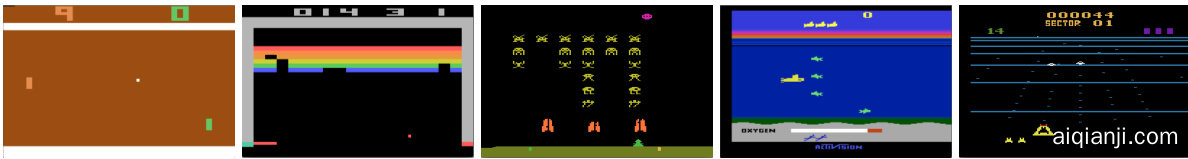
Figure 1: Screen shots from five Atari 2600 Games: (Left-to-right) Pong, Breakout, Space Invaders, Seaquest, Beam Rider

图 1: 五款Atari 2600游戏画面截图：(从左至右) Pong, Breakout, Space Invaders, Seaquest, Beam Rider

We apply our approach to a range of Atari 2600 games implemented in The Arcade Learning Environment (ALE) [3]. Atari 2600 is a challenging RL testbed that presents agents with a high dimensional visual input $(210\times160$ RGB video at $60\mathrm{Hz}$ ) and a diverse and interesting set of tasks that were designed to be difficult for humans players. Our goal is to create a single neural network agent that is able to successfully learn to play as many of the games as possible. The network was not provided with any game-specific information or hand-designed visual features, and was not privy to the internal state of the emulator; it learned from nothing but the video input, the reward and terminal signals, and the set of possible actions—just as a human player would. Furthermore the network architecture and all hyper parameters used for training were kept constant across the games. So far the network has outperformed all previous RL algorithms on six of the seven games we have attempted and surpassed an expert human player on three of them. Figure 1 provides sample screenshots from five of the games used for training.

我们将方法应用于一系列在街机学习环境 (ALE) [3] 中实现的 Atari 2600 游戏。Atari 2600 是一个具有挑战性的强化学习测试平台，它为智能体提供了高维视觉输入 $(210\times160$ RGB 视频，频率为 $60\mathrm{Hz}$ ) 以及一组多样且有趣的任务，这些任务设计初衷就是让人类玩家感到困难。我们的目标是创建一个单一的神经网络智能体，能够成功学习并尽可能多地掌握这些游戏。该网络没有获得任何游戏特定信息或手动设计的视觉特征，也无法访问模拟器的内部状态；它仅从视频输入、奖励和终止信号以及可能的动作集合中学习——就像人类玩家一样。此外，网络架构和所有训练使用的超参数在所有游戏中保持一致。截至目前，该网络在我们尝试的七款游戏中的六款上超越了所有先前的强化学习算法，并在其中三款游戏中超越了人类专家玩家。图 1 提供了用于训练的五款游戏的示例截图。

2 Background

2 背景

We consider tasks in which an agent interacts with an environment $\mathcal{E}$ , in this case the Atari emulator, in a sequence of actions, observations and rewards. At each time-step the agent selects an action $a_ {t}$ from the set of legal game actions, $\mathcal{A}={1,\ldots,K}$ . The action is passed to the emulator and modifies its internal state and the game score. In general $\mathcal{E}$ may be stochastic. The emulator’s internal state is not observed by the agent; instead it observes an image $\boldsymbol{x}_ {t}\in\mathbb{R}^{d}$ from the emulator, which is a vector of raw pixel values representing the current screen. In addition it receives a reward $r_ {t}$ representing the change in game score. Note that in general the game score may depend on the whole prior sequence of actions and observations; feedback about an action may only be received after many thousands of time-steps have elapsed.

我们考虑一种任务场景：AI智能体 (AI Agent) 与环境 $\mathcal{E}$（此处指Atari模拟器）通过一系列动作、观察和奖励进行交互。在每个时间步，智能体从合法游戏动作集合 $\mathcal{A}={1,\ldots,K}$ 中选择动作 $a_ {t}$。该动作被传递至模拟器，并改变其内部状态及游戏分数。通常 $\mathcal{E}$ 可能具有随机性。智能体无法观测模拟器的内部状态，仅能获取模拟器生成的图像 $\boldsymbol{x}_ {t}\in\mathbb{R}^{d}$——这是一个代表当前屏幕的原始像素值向量。同时，智能体会接收到反映游戏分数变化的奖励 $r_ {t}$。需要注意的是，游戏分数通常取决于先前所有动作和观察的序列，某个动作的反馈可能要在经历数千个时间步之后才能显现。

Since the agent only observes images of the current screen, the task is partially observed and many emulator states are perceptual ly aliased, i.e. it is impossible to fully understand the current situation from only the current screen $x_ {t}$ . We therefore consider sequences of actions and observations, $s_ {t}=$ $x_ {1},a_ {1},x_ {2},...,a_ {t-1},x_ {t}$ , and learn game strategies that depend upon these sequences. All sequences in the emulator are assumed to terminate in a finite number of time-steps. This formalism gives rise to a large but finite Markov decision process (MDP) in which each sequence is a distinct state. As a result, we can apply standard reinforcement learning methods for MDPs, simply by using the complete sequence $s_ {t}$ as the state representation at time $t$ .

由于智能体仅能观察到当前屏幕的图像，该任务属于部分可观测任务，且许多模拟器状态在感知上存在歧义，即仅凭当前屏幕 $x_ {t}$ 无法完全理解当前状况。因此，我们考虑动作与观测的序列 $s_ {t}=x_ {1},a_ {1},x_ {2},...,a_ {t-1},x_ {t}$ ，并学习依赖于这些序列的游戏策略。假设模拟器中所有序列都在有限时间步内终止。这种形式化方法产生了一个庞大但有限的马尔可夫决策过程 (MDP) ，其中每个序列都是一个独立的状态。如此一来，我们只需将完整序列 $s_ {t}$ 作为时间 $t$ 的状态表示，即可应用标准的 MDP 强化学习方法。

The goal of the agent is to interact with the emulator by selecting actions in a way that maximises future rewards. We make the standard assumption that future rewards are discounted by a factor of $\gamma$ per time-step, and define the future discounted return at time $t$ as $\begin{array}{r}{R_ {t}=\sum_ {t^{\prime}=t}^{T}\gamma^{t^{\prime}-t}r_ {t^{\prime}}}\end{array}$ γt′−trt′ , where T is the time-step at which the game terminates. We define the optimal actio n-value function $Q^{* }(s,a)$ as the maximum expected return achievable by following any strategy, after seeing some sequence $s$ and then taking some action $a$ , $Q^{* }(s,a)=\operatorname* {max}_ {\boldsymbol{\pi}}\mathbb{E}\left[R_ {t}|s_ {t}=s,a_ {t}=a,\boldsymbol{\pi}\right]$ , where $\pi$ is a policy mapping sequences to actions (or distributions over actions).

该智能体的目标是通过选择行动与模拟器交互，以最大化未来奖励。我们采用标准假设：未来奖励按每时间步长以系数 $\gamma$ 进行折现，并将时间 $t$ 的未来折现回报定义为 $\begin{array}{r}{R_ {t}=\sum_ {t^{\prime}=t}^{T}\gamma^{t^{\prime}-t}r_ {t^{\prime}}}\end{array}$ ，其中T为游戏终止的时间步长。最优动作-价值函数 $Q^{* }(s,a)$ 定义为在观察到某个序列 $s$ 并执行动作 $a$ 后，遵循任意策略所能获得的最大期望回报： $Q^{* }(s,a)=\operatorname* {max}_ {\boldsymbol{\pi}}\mathbb{E}\left[R_ {t}|s_ {t}=s,a_ {t}=a,\boldsymbol{\pi}\right]$ ，其中 $\pi$ 是将序列映射到动作（或动作分布）的策略。

The optimal action-value function obeys an important identity known as the Bellman equation. This is based on the following intuition: if the optimal value $Q^{* }(s^{\prime},a^{\prime})$ of the sequence $s^{\prime}$ at the next time-step was known for all possible actions $a^{\prime}$ , then the optimal strategy is to select the action $a^{\prime}$ maximising the expected value of $r+\gamma Q^{* }(s^{\prime},a^{\prime})$ ,

最优动作价值函数遵循一个被称为贝尔曼方程 (Bellman equation) 的重要恒等式。其核心思想是：若已知下一时间步所有可能动作 $a^{\prime}$ 对应的序列状态 $s^{\prime}$ 的最优值 $Q^{* }(s^{\prime},a^{\prime})$ ，则最优策略就是选择能最大化 $r+\gamma Q^{* }(s^{\prime},a^{\prime})$ 期望值的动作 $a^{\prime}$ 。

$$
\boldsymbol{Q}^{* }(s,a)=\mathbb{E}_ {s^{\prime}\sim\mathcal{E}}\left[r+\gamma\operatorname* {max}_ {a^{\prime}}\boldsymbol{Q}^{* }(s^{\prime},a^{\prime})\middle|s,a\right]
$$

$$
\boldsymbol{Q}^{* }(s,a)=\mathbb{E}_ {s^{\prime}\sim\mathcal{E}}\left[r+\gamma\operatorname* {max}_ {a^{\prime}}\boldsymbol{Q}^{* }(s^{\prime},a^{\prime})\middle|s,a\right]
$$

The basic idea behind many reinforcement learning algorithms is to estimate the actionvalue function, by using the Bellman equation as an iterative update, $\begin{array}{r l}{Q_ {i+1}(s,a)}&{{}=}\end{array}$ $\mathbb{E}\left[r+\gamma\operatorname* {max}_ {a^{\prime}}Q_ {i}(\dot{s}^{\prime},a^{\prime})|\dot{s},a\right]$ . Such value iteration algorithms converge to the optimal actionvalue function, $Q_ {i}\to Q^{* }$ as $i\rightarrow\infty$ [23]. In practice, this basic approach is totally impractical, because the action-value function is estimated separately for each sequence, without any generalisation. Instead, it is common to use a function approx im at or to estimate the action-value function, $Q(s,a;\theta)\approx Q^{* }(s,a)$ . In the reinforcement learning community this is typically a linear function approx im at or, but sometimes a non-linear function approx im at or is used instead, such as a neural network. We refer to a neural network function approx im at or with weights $\theta$ as a Q-network. A Q-network can be trained by minimising a sequence of loss functions $L_ {i}(\theta_ {i})$ that changes at each iteration $i$ ,

许多强化学习算法的基本思想是通过使用贝尔曼方程作为迭代更新来估计动作价值函数，$\begin{array}{r l}{Q_ {i+1}(s,a)}&{{}=}\end{array}$ $\mathbb{E}\left[r+\gamma\operatorname* {max}_ {a^{\prime}}Q_ {i}(\dot{s}^{\prime},a^{\prime})|\dot{s},a\right]$。这类值迭代算法会收敛到最优动作价值函数，即当$i\rightarrow\infty$时$Q_ {i}\to Q^{* }$[23]。实际上，这种基础方法完全不具备实用性，因为动作价值函数是单独为每个序列估计的，没有任何泛化性。因此，通常会使用一个函数逼近器来估计动作价值函数，即$Q(s,a;\theta)\approx Q^{* }(s,a)$。在强化学习领域，这通常是一个线性函数逼近器，但有时也会使用非线性函数逼近器，例如神经网络。我们将带有权重$\theta$的神经网络函数逼近器称为Q网络。Q网络可以通过最小化一系列在每次迭代$i$时变化的损失函数$L_ {i}(\theta_ {i})$来训练。

$$
L_ {i}\left(\theta_ {i}\right)=\mathbb{E}_ {s,a\sim\rho\left(\cdot\right)}\left[\left(y_ {i}-Q\left(s,a;\theta_ {i}\right)\right)^{2}\right],
$$

$$
L_ {i}\left(\theta_ {i}\right)=\mathbb{E}_ {s,a\sim\rho\left(\cdot\right)}\left[\left(y_ {i}-Q\left(s,a;\theta_ {i}\right)\right)^{2}\right],
$$

where $y_ {i}=\mathbb{E}_ {s^{\prime}\sim\mathcal{E}}[r+\gamma\operatorname* {max}_ {a^{\prime}}Q(s^{\prime},a^{\prime};\theta_ {i-1})|s,a]$ is the target for iteration $i$ and $\rho(s,a)$ is a probability distribution over sequences $s$ and actions $a$ that we refer to as the behaviour distribution. The parameters from the previous iteration $\theta_ {i-1}$ are held fixed when optimising the loss function $L_ {i}\left(\theta_ {i}\right)$ . Note that the targets depend on the network weights; this is in contrast with the targets used for supervised learning, which are fixed before learning begins. Differentiating the loss function with respect to the weights we arrive at the following gradient,

其中 $y_ {i}=\mathbb{E}_ {s^{\prime}\sim\mathcal{E}}[r+\gamma\operatorname* {max}_ {a^{\prime}}Q(s^{\prime},a^{\prime};\theta_ {i-1})|s,a]$ 是第 $i$ 次迭代的目标值，$\rho(s,a)$ 是状态序列 $s$ 和动作 $a$ 的概率分布（我们称之为行为分布）。在优化损失函数 $L_ {i}\left(\theta_ {i}\right)$ 时，前次迭代的参数 $\theta_ {i-1}$ 保持固定。需要注意的是，这些目标值依赖于网络权重——这与监督学习中使用的固定预设目标不同。对损失函数进行权重求导可得如下梯度：

$$
\nabla_ {\theta_ {i}}L_ {i}\left(\theta_ {i}\right)=\mathbb{E}_ {s,a\sim\rho\left(\cdot\right);s^{\prime}\sim\mathcal{E}}\left[\left(r+\gamma\operatorname* {max}_ {a^{\prime}}Q(s^{\prime},a^{\prime};\theta_ {i-1})-Q(s,a;\theta_ {i})\right)\nabla_ {\theta_ {i}}Q(s,a;\theta_ {i})\right].
$$

$$
\nabla_ {\theta_ {i}}L_ {i}\left(\theta_ {i}\right)=\mathbb{E}_ {s,a\sim\rho\left(\cdot\right);s^{\prime}\sim\mathcal{E}}\left[\left(r+\gamma\operatorname* {max}_ {a^{\prime}}Q(s^{\prime},a^{\prime};\theta_ {i-1})-Q(s,a;\theta_ {i})\right)\nabla_ {\theta_ {i}}Q(s,a;\theta_ {i})\right].
$$

Rather than computing the full expectations in the above gradient, it is often computationally expedient to optimise the loss function by stochastic gradient descent. If the weights are updated after every time-step, and the expectations are replaced by single samples from the behaviour distribution $\rho$ and the emulator $\mathcal{E}$ respectively, then we arrive at the familiar $Q$ -learning algorithm [26].

相较于计算上述梯度中的完整期望值，通过随机梯度下降优化损失函数通常在计算上更为便捷。若在每个时间步后更新权重，并将期望值分别替换为行为分布 $\rho$ 和模拟器 $\mathcal{E}$ 的单个样本，即可得到经典的 $Q$ 学习算法 [26]。

Note that this algorithm is model-free: it solves the reinforcement learning task directly using samples from the emulator $\mathcal{E}$ , without explicitly constructing an estimate of $\mathcal{E}$ . It is also off-policy: it learns about the greedy strategy $a=\operatorname* {max}_ {a}Q(s,a;\theta)$ , while following a behaviour distribution that ensures adequate exploration of the state space. In practice, the behaviour distribution is often selected by an $\epsilon$ -greedy strategy that follows the greedy strategy with probability $1-\epsilon$ and selects a random action with probability $\epsilon$ .

需要注意的是，该算法是无模型(model-free)的：它直接使用模拟器$\mathcal{E}$的样本来解决强化学习任务，而无需显式构建对$\mathcal{E}$的估计。它同时也是离策略(off-policy)的：在学习贪婪策略$a=\operatorname* {max}_ {a}Q(s,a;\theta)$的同时，遵循一个确保充分探索状态空间的行为分布。实践中，行为分布通常采用$\epsilon$-贪婪策略来选择，即以$1-\epsilon$的概率遵循贪婪策略，以$\epsilon$的概率随机选择动作。

3 Related Work

3 相关工作

Perhaps the best-known success story of reinforcement learning is $T D$ -gammon, a backgammonplaying program which learnt entirely by reinforcement learning and self-play, and achieved a superhuman level of play [24]. TD-gammon used a model-free reinforcement learning algorithm similar to Q-learning, and approximated the value function using a multi-layer perceptron with one hidden layer1.

强化学习最著名的成功案例或许是TD-Gammon这款西洋双陆棋程序，它完全通过强化学习和自我对弈进行训练，并达到了超越人类水平的棋力[24]。TD-Gammon采用了与Q学习类似的无模型强化学习算法，并通过带有一个隐藏层的多层感知机来近似价值函数1。

However, early attempts to follow up on TD-gammon, including applications of the same method to chess, Go and checkers were less successful. This led to a widespread belief that the TD-gammon approach was a special case that only worked in backgammon, perhaps because the stochastic it y in the dice rolls helps explore the state space and also makes the value function particularly smooth [19].

然而，后续对TD-gammon的早期尝试，包括将该方法应用于国际象棋、围棋和跳棋时，效果并不理想。这导致人们普遍认为TD-gammon方法是一个特例，仅适用于双陆棋，或许是因为骰子的随机性有助于探索状态空间，同时也使价值函数特别平滑 [19]。

Furthermore, it was shown that combining model-free reinforcement learning algorithms such as Qlearning with non-linear function ap proxima tors [25], or indeed with off-policy learning [1] could cause the Q-network to diverge. Subsequently, the majority of work in reinforcement learning focused on linear function ap proxima tors with better convergence guarantees [25].

此外，研究表明，将Qlearning等无模型强化学习算法与非线性函数逼近器[25]结合，或者实际采用离策略学习[1]时，可能导致Q网络发散。随后，大多数强化学习研究转向了具有更好收敛保证的线性函数逼近器[25]。

More recently, there has been a revival of interest in combining deep learning with reinforcement learning. Deep neural networks have been used to estimate the environment $\mathcal{E}$ ; restricted Boltzmann machines have been used to estimate the value function [21]; or the policy [9]. In addition, the divergence issues with Q-learning have been partially addressed by gradient temporal-difference methods. These methods are proven to converge when evaluating a fixed policy with a nonlinear function approx im at or [14]; or when learning a control policy with linear function approximation using a restricted variant of Q-learning [15]. However, these methods have not yet been extended to nonlinear control.

最近，深度学习与强化学习相结合的领域重新引起了人们的兴趣。深度神经网络被用于估计环境 $\mathcal{E}$；受限玻尔兹曼机被用于估计价值函数 [21] 或策略 [9]。此外，Q学习的发散问题已通过梯度时间差分方法得到部分解决。这些方法在评估固定策略时（使用非线性函数近似器 [14]）或学习控制策略时（使用线性函数近似的Q学习受限变体 [15]）被证明是收敛的。然而，这些方法尚未扩展到非线性控制领域。

Perhaps the most similar prior work to our own approach is neural fitted Q-learning (NFQ) [20]. NFQ optimises the sequence of loss functions in Equation 2, using the RPROP algorithm to update the parameters of the Q-network. However, it uses a batch update that has a computational cost per iteration that is proportional to the size of the data set, whereas we consider stochastic gradient updates that have a low constant cost per iteration and scale to large data-sets. NFQ has also been successfully applied to simple real-world control tasks using purely visual input, by first using deep auto encoders to learn a low dimensional representation of the task, and then applying NFQ to this representation [12]. In contrast our approach applies reinforcement learning end-to-end, directly from the visual inputs; as a result it may learn features that are directly relevant to discriminating action-values. Q-learning has also previously been combined with experience replay and a simple neural network [13], but again starting with a low-dimensional state rather than raw visual inputs.

与我们方法最为相似的先前工作可能是神经拟合Q学习 (neural fitted Q-learning, NFQ) [20]。NFQ通过RPROP算法更新Q网络参数来优化公式2中的损失函数序列。但该方法采用批量更新方式，每次迭代的计算成本与数据集大小成正比，而我们采用随机梯度更新，每次迭代的计算成本较低且能扩展到大型数据集。NFQ还通过先使用深度自动编码器学习任务的低维表示，再对其应用NFQ [12]，成功实现了纯视觉输入的简单现实控制任务。相比之下，我们的方法直接从视觉输入端到端地应用强化学习，因此可能学习到与动作价值判别直接相关的特征。Q学习此前也曾与经验回放和简单神经网络结合使用 [13]，但同样是从低维状态而非原始视觉输入开始。

The use of the Atari 2600 emulator as a reinforcement learning platform was introduced by [3], who applied standard reinforcement learning algorithms with linear function approximation and generic visual features. Subsequently, results were improved by using a larger number of features, and using tug-of-war hashing to randomly project the features into a lower-dimensional space [2]. The HyperNEAT evolutionary architecture [8] has also been applied to the Atari platform, where it was used to evolve (separately, for each distinct game) a neural network representing a strategy for that game. When trained repeatedly against deterministic sequences using the emulator’s reset facility, these strategies were able to exploit design flaws in several Atari games.

[3] 首次将 Atari 2600 模拟器作为强化学习平台，他们采用线性函数逼近和通用视觉特征的标准强化学习算法。随后，通过使用更多特征以及利用 tug-of-war 哈希将特征随机投影到低维空间 [2]，结果得到了改善。HyperNEAT 进化架构 [8] 也被应用于 Atari 平台，用于针对每个不同游戏分别进化出代表该游戏策略的神经网络。当通过模拟器的重置功能反复针对确定性序列进行训练时，这些策略能够利用多款 Atari 游戏中的设计缺陷。

4 Deep Reinforcement Learning

4 深度强化学习

Recent breakthroughs in computer vision and speech recognition have relied on efficiently training deep neural networks on very large training sets. The most successful approaches are trained directly from the raw inputs, using lightweight updates based on stochastic gradient descent. By feeding sufficient data into deep neural networks, it is often possible to learn better representations than handcrafted features [11]. These successes motivate our approach to reinforcement learning. Our goal is to connect a reinforcement learning algorithm to a deep neural network which operates directly on RGB images and efficiently process training data by using stochastic gradient updates.

计算机视觉和语音识别领域的最新突破，依赖于在超大规模训练集上高效训练深度神经网络。最成功的方法直接从原始输入进行训练，采用基于随机梯度下降的轻量级更新机制。通过向深度神经网络输入足够数据，通常能学习到比手工特征更优的表征 [11]。这些成果启发了我们强化学习的研究路径。我们的目标是将强化学习算法与深度神经网络相连，使其直接处理RGB图像，并通过随机梯度更新高效处理训练数据。

Tesauro’s TD-Gammon architecture provides a starting point for such an approach. This architecture updates the parameters of a network that estimates the value function, directly from on-policy samples of experience, $s_ {t},a_ {t},r_ {t},s_ {t+1},a_ {t+1}$ , drawn from the algorithm’s interactions with the environment (or by self-play, in the case of backgammon). Since this approach was able to outperform the best human backgammon players 20 years ago, it is natural to wonder whether two decades of hardware improvements, coupled with modern deep neural network architectures and scalable RL algorithms might produce significant progress.

Tesauro 的 TD-Gammon 架构为这种方法提供了起点。该架构通过算法与环境交互 (或双陆棋中的自我对弈) 获得的策略样本经验 $s_ {t},a_ {t},r_ {t},s_ {t+1},a_ {t+1}$ ，直接更新价值函数估计网络的参数。由于这种方法在 20 年前就能超越最优秀的人类双陆棋选手，人们自然会思考：二十年的硬件进步结合现代深度神经网络架构和可扩展的强化学习算法，是否能带来重大突破。

In contrast to TD-Gammon and similar online approaches, we utilize a technique known as experience replay [13] where we store the agent’s experiences at each time-step, $e_ {t}=\left(s_ {t},a_ {t},r_ {t},s_ {t+1}\right)$ in a data-set $\mathcal{D}=e_ {1},...,e_ {N}$ , pooled over many episodes into a replay memory. During the inner loop of the algorithm, we apply Q-learning updates, or minibatch updates, to samples of experience, $e\sim D$ , drawn at random from the pool of stored samples. After performing experience replay, the agent selects and executes an action according to an $\epsilon$ -greedy policy. Since using histories of arbitrary length as inputs to a neural network can be difficult, our Q-function instead works on fixed length representation of histories produced by a function $\phi$ . The full algorithm, which we call deep $Q$ -learning, is presented in Algorithm 1.

与TD-Gammon等在线方法不同，我们采用了一种称为经验回放[13]的技术，将智能体在每个时间步的经历 $e_ {t}=\left(s_ {t},a_ {t},r_ {t},s_ {t+1}\right)$ 存储在数据集 $\mathcal{D}=e_ {1},...,e_ {N}$ 中，并将多轮次数据汇集成回放记忆库。在算法的内循环中，我们对从存储样本池中随机抽取的经验样本 $e\sim D$ 应用Q学习更新或小批量更新。完成经验回放后，智能体根据 $\epsilon$ -贪婪策略选择并执行动作。由于将任意长度的历史记录作为神经网络输入较为困难，我们的Q函数改为处理由函数 $\phi$ 生成的固定长度历史表示。完整算法（我们称之为深度 $Q$ 学习）如算法1所示。

This approach has several advantages over standard online Q-learning [23]. First, each step of experience is potentially used in many weight updates, which allows for greater data efficiency.

这种方法相比标准的在线Q学习[23]具有多个优势。首先，每个经验步骤都可能用于多次权重更新，从而提高了数据利用效率。

Initialize replay memory D to capacity N Initialize action-value function Q with random weights for episode = 1, M do

Initialise sequence s1 = {1} and preprocessed sequenced Φ1 = Φ(s1)

for t = 1, T do With probability E select a random action at

otherwise select at = maxa Q* (Φ(st),a; 0)

Execute action at in emulator and observe reward rt and image Xt+1

Set St+1 = St, at, Ct+1 and preprocess Φt+1 = Φ(st+1)

Store transition (Φt, at, rt, Φt+1) in D

Sample random minibatch of transitions (Φ§, a, r§, Φj+1) from D

for terminal Φ+1 Set yj rj

rj + maxa Q(Φ+1,a';0) for non-terminal Φj+1

Perform a gradient descent step on (yj - Q(Φ, a; 0)2 according to equation 3

end for end for

| 初始化回放记忆库 D，容量为 N |
| 用随机权重初始化动作价值函数 Q |
| 对于每个回合 episode = 1 到 M 执行 |
| 初始化序列 s1 = {1} 并预处理序列 Φ1 = Φ(s1) |
| 对于每个时间步 t = 1 到 T 执行 |
| 以概率 ε 随机选择动作 at |
| 否则选择 at = maxa Q* (Φ(st), a; θ) |
| 在模拟器中执行动作 at，观察奖励 rt 和图像 Xt+1 |
| 设置 st+1 = st, at, xt+1 并预处理 Φt+1 = Φ(st+1) |
| 将转移 (Φt, at, rt, Φt+1) 存入 D |
| 从 D 中随机采样小批量转移 (Φj, aj, rj, Φj+1) |
| 对于终止状态的 Φj+1 设置 yj = rj |
| 对于非终止状态的 Φj+1 设置 yj = rj + γ maxa' Q(Φj+1, a'; θ) |
| 根据方程 3 对 (yj - Q(Φj, aj; θ))^2 执行梯度下降步骤 |
| 结束循环 |

Second, learning directly from consecutive samples is inefficient, due to the strong correlations between the samples; randomizing the samples breaks these correlations and therefore reduces the variance of the updates. Third, when learning on-policy the current parameters determine the next data sample that the parameters are trained on. For example, if the maximizing action is to move left then the training samples will be dominated by samples from the left-hand side; if the maximizing action then switches to the right then the training distribution will also switch. It is easy to see how unwanted feedback loops may arise and the parameters could get stuck in a poor local minimum, or even diverge catastrophically [25]. By using experience replay the behavior distribution is averaged over many of its previous states, smoothing out learning and avoiding oscillations or divergence in the parameters. Note that when learning by experience replay, it is necessary to learn off-policy (because our current parameters are different to those used to generate the sample), which motivates the choice of Q-learning.

其次，直接从连续样本中学习效率低下，因为样本之间存在强相关性；随机化样本能打破这些关联，从而降低更新的方差。第三，在策略学习时，当前参数决定了训练参数的下一批数据样本。例如，若最大化动作是向左移动，则训练样本会主要来自左侧；若最大化动作随后转为向右，训练数据分布也会随之改变。这容易引发不良反馈循环，导致参数陷入局部极小值，甚至出现灾难性发散 [25]。通过经验回放，行为分布会在多个先前状态上取平均，从而平滑学习过程并避免参数振荡或发散。需要注意的是，使用经验回放学习时必须采用离策略方式（因为当前参数与生成样本时所用参数不同），这正是选择Q学习算法的动机所在。

In practice, our algorithm only stores the last $N$ experience tuples in the replay memory, and samples uniformly at random from $\mathcal{D}$ when performing updates. This approach is in some respects limited since the memory buffer does not differentiate important transitions and always overwrites with recent transitions due to the finite memory size $N$ . Similarly, the uniform sampling gives equal importance to all transitions in the replay memory. A more sophisticated sampling strategy might emphasize transitions from which we can learn the most, similar to prioritized sweeping [17].

在实践中，我们的算法仅存储最近 $N$ 条经验元组到回放内存中，并在执行更新时从 $\mathcal{D}$ 中均匀随机采样。这种方法在某些方面存在局限，因为内存缓冲区不会区分重要转移，且由于有限内存大小 $N$ 总是用最新转移覆盖旧数据。同样，均匀采样赋予回放内存中所有转移相同的权重。更复杂的采样策略可能会强调那些我们能从中学习最多的转移，类似于优先扫描 [17]。

4.1 Preprocessing and Model Architecture

4.1 预处理与模型架构

Working directly with raw Atari frames, which are $210\times160$ pixel images with a 128 color palette, can be computationally demanding, so we apply a basic preprocessing step aimed at reducing the input dimensionality. The raw frames are pre processed by first converting their RGB representation to gray-scale and down-sampling it to a $110\times84$ image. The final input representation is obtained by cropping an $84\times84$ region of the image that roughly captures the playing area. The final cropping stage is only required because we use the GPU implementation of 2D convolutions from [11], which expects square inputs. For the experiments in this paper, the function $\phi$ from algorithm 1 applies this preprocessing to the last 4 frames of a history and stacks them to produce the input to the $Q$ -function.

直接处理原始的Atari帧（即128色调色板的$210\times160$像素图像）对计算资源要求较高，因此我们采用了一个基础预处理步骤来降低输入维度。原始帧首先从RGB格式转换为灰度图像，并下采样至$110\times84$尺寸。最终输入表示是通过截取图像中$84\times84$的近似游戏区域获得的。最后一步裁剪仅因我们使用了[11]中基于GPU的二维卷积实现（该实现要求输入为方形）。本文实验中，算法1的函数$\phi$会对历史序列的最后4帧进行上述预处理，并将其堆叠作为$Q$函数的输入。

There are several possible ways of parameter i zing $Q$ using a neural network. Since $Q$ maps historyaction pairs to scalar estimates of their Q-value, the history and the action have been used as inputs to the neural network by some previous approaches [20, 12]. The main drawback of this type of architecture is that a separate forward pass is required to compute the $\mathsf{Q}.$ -value of each action, resulting in a cost that scales linearly with the number of actions. We instead use an architecture in which there is a separate output unit for each possible action, and only the state representation is an input to the neural network. The outputs correspond to the predicted Q-values of the individual action for the input state. The main advantage of this type of architecture is the ability to compute Q-values for all possible actions in a given state with only a single forward pass through the network.

使用神经网络对 $Q$ 进行参数化有几种可能的方式。由于 $Q$ 将历史-动作对映射到其Q值的标量估计，一些先前的方法 [20, 12] 将历史和动作作为神经网络的输入。这类架构的主要缺点是，需要单独的前向传递来计算每个动作的 $\mathsf{Q}$ 值，导致计算成本随动作数量线性增长。我们采用了一种不同的架构，其中每个可能的动作都有一个单独的输出单元，只有状态表示作为神经网络的输入。输出对应于输入状态下各个动作的预测Q值。这类架构的主要优势是能够通过单次前向传递计算给定状态下所有可能动作的Q值。

We now describe the exact architecture used for all seven Atari games. The input to the neural network consists is an $84\times84\times4$ image produced by $\phi$ . The first hidden layer convolves $168\times8$ filters with stride 4 with the input image and applies a rectifier non linearity [10, 18]. The second hidden layer convolves $324\times4$ filters with stride 2, again followed by a rectifier non linearity. The final hidden layer is fully-connected and consists of 256 rectifier units. The output layer is a fullyconnected linear layer with a single output for each valid action. The number of valid actions varied between 4 and 18 on the games we considered. We refer to convolutional networks trained with our approach as Deep Q-Networks (DQN).

我们现在描述用于所有七款Atari游戏的精确架构。神经网络的输入是由$\phi$生成的$84\times84\times4$图像。第一个隐藏层使用16个$8\times8$滤波器以步长4对输入图像进行卷积，并应用整流非线性激活函数[10, 18]。第二个隐藏层使用32个$4\times4$滤波器以步长2进行卷积，同样后接整流非线性激活函数。最后的隐藏层是全连接的，包含256个整流单元。输出层是一个全连接线性层，每个有效动作对应一个输出。在我们考虑的游戏中，有效动作数量从4到18不等。我们将采用该方法训练的卷积网络称为深度Q网络(DQN)。

5 Experiments

5 实验

So far, we have performed experiments on seven popular ATARI games – Beam Rider, Breakout, Enduro, Pong, $\mathrm{Q}^{* }$ bert, Seaquest, Space Invaders. We use the same network architecture, learning algorithm and hyper parameters settings across all seven games, showing that our approach is robust enough to work on a variety of games without incorporating game-specific information. While we evaluated our agents on the real and unmodified games, we made one change to the reward structure of the games during training only. Since the scale of scores varies greatly from game to game, we fixed all positive rewards to be 1 and all negative rewards to be $-1$ , leaving 0 rewards unchanged. Clipping the rewards in this manner limits the scale of the error derivatives and makes it easier to use the same learning rate across multiple games. At the same time, it could affect the performance of our agent since it cannot differentiate between rewards of different magnitude.

目前，我们已在七款经典ATARI游戏(Beam Rider、Breakout、Enduro、Pong、$\mathrm{Q}^{* }$bert、Seaquest、Space Invaders)上完成实验。所有游戏采用相同的网络架构、学习算法和超参数设置，这表明我们的方法具有足够鲁棒性，无需引入游戏特定信息即可适应多种游戏。虽然我们在原始未修改版本上评估AI智能体，但在训练阶段对游戏奖励结构做了一项调整：鉴于不同游戏的分数范围差异巨大，我们将所有正向奖励固定为1，负向奖励设为$-1$，零奖励保持不变。这种奖励截断机制限制了误差导数的规模，使得跨游戏使用相同学习率成为可能。但这也可能导致智能体无法区分不同量级的奖励，从而影响其性能表现。

In these experiments, we used the RMSProp algorithm with mini batches of size 32. The behavior policy during training was $\epsilon$ -greedy with $\epsilon$ annealed linearly from 1 to 0.1 over the first million frames, and fixed at 0.1 thereafter. We trained for a total of 10 million frames and used a replay memory of one million most recent frames.

在这些实验中，我们使用了批量为32的RMSProp算法。训练期间的行为策略采用$\epsilon$-贪婪算法，$\epsilon$在前100万帧中从1线性退火至0.1，之后固定为0.1。我们总共训练了1000万帧，并使用了一个存储最近100万帧的经验回放池。

Following previous approaches to playing Atari games, we also use a simple frame-skipping technique [3]. More precisely, the agent sees and selects actions on every $k^{t\hat{h}}$ frame instead of every frame, and its last action is repeated on skipped frames. Since running the emulator forward for one step requires much less computation than having the agent select an action, this technique allows the agent to play roughly $k$ times more games without significantly increasing the runtime. We use $k=4$ for all games except Space Invaders where we noticed that using $k=4$ makes the lasers invisible because of the period at which they blink. We used $k=3$ to make the lasers visible and this change was the only difference in hyper parameter values between any of the games.

遵循先前玩Atari游戏的方法，我们也采用了一种简单的跳帧技术[3]。具体来说，智能体每隔$k^{t\hat{h}}$帧观察并选择动作，而非每帧都操作，跳过的帧会重复其上一个动作。由于模拟器前进一步所需的计算量远小于智能体选择动作的计算量，该技术能让智能体在不显著增加运行时间的情况下，多玩大约$k$倍的游戏。除《太空侵略者》外，所有游戏均使用$k=4$。在该游戏中，我们发现$k=4$会导致激光因闪烁周期而不可见，因此改用$k=3$使激光可见。这一调整是所有游戏间唯一的超参数差异。

5.1 Training and Stability

5.1 训练与稳定性

In supervised learning, one can easily track the performance of a model during training by evaluating it on the training and validation sets. In reinforcement learning, however, accurately evaluating the progress of an agent during training can be challenging. Since our evaluation metric, as suggested by [3], is the total reward the agent collects in an episode or game averaged over a number of games, we periodically compute it during training. The average total reward metric tends to be very noisy because small changes to the weights of a policy can lead to large changes in the distribution of states the policy visits . The leftmost two plots in figure 2 show how the average total reward evolves during training on the games Seaquest and Breakout. Both averaged reward plots are indeed quite noisy, giving one the impression that the learning algorithm is not making steady progress. Another, more stable, metric is the policy’s estimated action-value function $Q$ , which provides an estimate of how much discounted reward the agent can obtain by following its policy from any given state. We collect a fixed set of states by running a random policy before training starts and track the average of the maximum2 predicted $Q$ for these states. The two rightmost plots in figure 2 show that average predicted $Q$ increases much more smoothly than the average total reward obtained by the agent and plotting the same metrics on the other five games produces similarly smooth curves. In addition to seeing relatively smooth improvement to predicted $Q$ during training we did not experience any divergence issues in any of our experiments. This suggests that, despite lacking any theoretical convergence guarantees, our method is able to train large neural networks using a reinforcement learning signal and stochastic gradient descent in a stable manner.

在监督学习中，通过评估训练集和验证集上的表现，可以轻松追踪模型在训练期间的性能。然而在强化学习中，准确评估智能体在训练过程中的进展可能颇具挑战性。根据[3]的建议，我们的评估指标是智能体在多轮游戏或对局中获得的总奖励平均值，因此在训练期间会定期计算该指标。平均总奖励指标往往存在较大波动，因为策略权重的微小变化可能导致该策略访问的状态分布发生显著改变。图2最左侧的两个图表展示了《海底探险》和《打砖块》游戏中平均总奖励在训练期间的变化情况。这两个平均奖励图表确实表现出明显波动，容易让人误认为学习算法没有取得稳定进展。

另一个更稳定的指标是策略的预估动作价值函数$Q$，它能估算智能体从任意给定状态开始遵循当前策略所能获得的折后奖励。我们在训练开始前通过运行随机策略收集一组固定状态，并跟踪这些状态下最大预测$Q$值的平均值。图2最右侧的两个图表显示，平均预测$Q$值的增长曲线比智能体获得的平均总奖励平滑得多，在其他五款游戏中绘制相同指标也产生了类似的平滑曲线。除了观察到预测$Q$值在训练期间相对平稳的提升外，我们在所有实验中均未遇到任何发散问题。这表明尽管缺乏理论收敛保证，我们的方法仍能通过强化学习信号和随机梯度下降稳定地训练大型神经网络。

Figure 2: The two plots on the left show average reward per episode on Breakout and Seaquest respectively during training. The statistics were computed by running an $\epsilon$ -greedy policy with $\epsilon=$ 0.05 for 10000 steps. The two plots on the right show the average maximum predicted action-value of a held out set of states on Breakout and Seaquest respectively. One epoch corresponds to 50000 minibatch weight updates or roughly 30 minutes of training time.

图 2: 左侧两幅图分别展示了训练期间Breakout和Seaquest游戏中每回合的平均奖励。统计数据是通过运行$\epsilon$-贪婪策略 ($\epsilon=$ 0.05) 进行10000步计算得出的。右侧两幅图分别显示了Breakout和Seaquest游戏中保留状态集的平均最大预测动作值。一个训练周期相当于50000次小批量权重更新或约30分钟的训练时间。

Figure 3: The leftmost plot shows the predicted value function for a 30 frame segment of the game Seaquest. The three screenshots correspond to the frames labeled by A, B, and C respectively.

图 3: 最左侧图表展示了游戏《海战》(Seaquest) 30帧片段的预测价值函数。三张截图分别对应标记为A、B和C的帧。

5.2 Visualizing the Value Function

5.2 价值函数可视化

Figure 3 shows a visualization of the learned value function on the game Seaquest. The figure shows that the predicted value jumps after an enemy appears on the left of the screen (point A). The agent then fires a torpedo at the enemy and the predicted value peaks as the torpedo is about to hit the enemy (point B). Finally, the value falls to roughly its original value after the enemy disappears (point C). Figure 3 demonstrates that our method is able to learn how the value function evolves for a reasonably complex sequence of events.

图 3: 展示了游戏《海战》(Seaquest)中学习到的价值函数可视化结果。该图显示当敌人在屏幕左侧出现时(点A)，预测价值会突然上升。随后智能体向敌人发射鱼雷，当鱼雷即将击中敌人时(点B)，预测价值达到峰值。最终，在敌人消失后(点C)，价值回落至接近初始水平。图3表明我们的方法能够学习价值函数在相对复杂事件序列中的演变规律。

5.3 Main Evaluation

5.3 主要评估

We compare our results with the best performing methods from the RL literature [3, 4]. The method labeled Sarsa used the Sarsa algorithm to learn linear policies on several different feature sets handengineered for the Atari task and we report the score for the best performing feature set [3]. Contingency used the same basic approach as Sarsa but augmented the feature sets with a learned representation of the parts of the screen that are under the agent’s control [4]. Note that both of these methods incorporate significant prior knowledge about the visual problem by using background subtraction and treating each of the 128 colors as a separate channel. Since many of the Atari games use one distinct color for each type of object, treating each color as a separate channel can be similar to producing a separate binary map encoding the presence of each object type. In contrast, our agents only receive the raw RGB screenshots as input and must learn to detect objects on their own.

我们将结果与强化学习文献中表现最佳的方法进行了比较 [3, 4]。标注为 Sarsa 的方法使用 Sarsa 算法学习针对 Atari 任务手工设计的多组不同特征集的线性策略，我们报告了表现最佳特征集的得分 [3]。Contingency 方法与 Sarsa 采用相同的基础方法，但通过添加对智能体控制屏幕区域的学习表示来增强特征集 [4]。需要注意的是，这两种方法都通过背景差分处理并将 128 种颜色分别作为独立通道，融入了大量关于视觉问题的先验知识。由于许多 Atari 游戏为每种对象类型使用独特颜色，将每种颜色作为独立通道处理类似于生成编码各对象类型存在的独立二值图。相比之下，我们的智能体仅接收原始 RGB 屏幕截图作为输入，必须自行学习检测对象。

In addition to the learned agents, we also report scores for an expert human game player and a policy that selects actions uniformly at random. The human performance is the median reward achieved after around two hours of playing each game. Note that our reported human scores are much higher than the ones in Bellemare et al. [3]. For the learned methods, we follow the evaluation strategy used in Bellemare et al. [3, 5] and report the average score obtained by running an $\epsilon\cdot$ -greedy policy with $\epsilon=0.05$ for a fixed number of steps. The first five rows of table 1 show the per-game average scores on all games. Our approach (labeled DQN) outperforms the other learning methods by a substantial margin on all seven games despite incorporating almost no prior knowledge about the inputs.

除了学习型智能体外，我们还记录了专业人类玩家和随机均匀选择动作策略的得分。人类表现数据来源于每位玩家在约两小时游戏后获得的中位数奖励值。需注意，本文报告的人类得分显著高于Bellemare等人[3]的研究结果。对于学习型方法，我们沿用Bellemare等人[3,5]的评估策略，报告通过运行$\epsilon=0.05$的$\epsilon\cdot$贪婪策略固定步数后获得的平均分。表1前五行展示了所有游戏的平均得分。尽管几乎未引入任何先验输入知识，我们的方法（标记为DQN）在全部七款游戏中均以显著优势超越其他学习方法。

We also include a comparison to the evolutionary policy search approach from [8] in the last three rows of table 1. We report two sets of results for this method. The HNeat Best score reflects the results obtained by using a hand-engineered object detector algorithm that outputs the locations and types of objects on the Atari screen. The HNeat Pixel score is obtained by using the special 8 color channel representation of the Atari emulator that represents an object label map at each channel. This method relies heavily on finding a deterministic sequence of states that represents a successful exploit. It is unlikely that strategies learnt in this way will generalize to random perturbations; therefore the algorithm was only evaluated on the highest scoring single episode. In contrast, our algorithm is evaluated on $\epsilon$ -greedy control sequences, and must therefore generalize across a wide variety of possible situations. Nevertheless, we show that on all the games, except Space Invaders, not only our max evaluation results (row 8), but also our average results (row 4) achieve better performance.

我们还在表1的最后三行加入了与文献[8]中进化策略搜索方法的对比。针对该方法报告了两组结果：HNeat Best分数是通过使用手工设计的物体检测算法获得的，该算法输出Atari屏幕上物体的位置和类型；HNeat Pixel分数则是利用Atari模拟器的特殊8色彩通道表示法（每个通道代表一个物体标签图）得出的。该方法高度依赖寻找代表成功利用的确定性状态序列，因此这种学习策略难以推广到随机扰动场景，故仅评估了单次最高分回合。相比之下，我们的算法在$\epsilon$-贪婪控制序列上进行评估，必须适应各种可能情境。尽管如此，数据显示除《太空侵略者》外，我们的最大评估结果（第8行）和平均结果（第4行）在所有游戏上都表现更优。

Table 1: The upper table compares average total reward for various learning methods by running an $\epsilon$ -greedy policy with $\epsilon=0.05$ for a fixed number of steps. The lower table reports results of the single best performing episode for HNeat and DQN. HNeat produces deterministic policies that always get the same score while DQN used an $\epsilon$ -greedy policy with $\epsilon=0.05$ .

	B. Rider	Breakout	Enduro	Pong	Q* bert	Seaquest	S.Invaders
Random	354	1.2	0	-20.4	157	110	179
Sarsa [3]	996	5.2	129	-19	614	665	271
Contingency[4]	1743	6	159	-17	960	723	268
DQN	4092	168	470	20	1952	1705	581
Human	7456	31	368	-3	18900	28010	3690
HNeatBest[8]	3616	52	106	19	1800	920	1720
HNeatPixel[8]	1332	4	91	-16	1325	800	1145
DQN Best	5184	225	661	21	4500	1740	1075

表 1: 上表比较了各种学习方法在固定步数下运行 $\epsilon$ -贪婪策略 ( $\epsilon=0.05$ ) 获得的平均总奖励。下表报告了 HNeat 和 DQN 单次最佳表现回合的结果。HNeat 生成确定性策略，始终获得相同分数，而 DQN 使用 $\epsilon$ -贪婪策略 ( $\epsilon=0.05$ ) 。

	B. Rider	Breakout	Enduro	Pong	Q* bert	Seaquest	S.Invaders
Random	354	1.2	0	-20.4	157	110	179
Sarsa [3]	996	5.2	129	-19	614	665	271
Contingency[4]	1743	6	159	-17	960	723	268
DQN	4092	168	470	20	1952	1705	581
Human	7456	31	368	-3	18900	28010	3690
HNeatBest[8]	3616	52	106	19	1800	920	1720
HNeatPixel[8]	1332	4	91	-16	1325	800	1145
DQN Best	5184	225	661	21	4500	1740	1075

Finally, we show that our method achieves better performance than an expert human player on Breakout, Enduro and Pong and it achieves close to human performance on Beam Rider. The games Q* bert, Seaquest, Space Invaders, on which we are far from human performance, are more challenging because they require the network to find a strategy that extends over long time scales.

最后，我们证明该方法在《Breakout》《Enduro》和《Pong》上的表现优于人类专家玩家，在《Beam Rider》上则接近人类水平。而在《Q* bert》《Seaquest》《Space Invaders》这些我们远未达到人类水平的游戏中，挑战更大，因为它们需要网络找到一种能长时间持续的策略。

6 Conclusion

6 结论

This paper introduced a new deep learning model for reinforcement learning, and demonstrated its ability to master difficult control policies for Atari 2600 computer games, using only raw pixels as input. We also presented a variant of online Q-learning that combines stochastic minibatch updates with experience replay memory to ease the training of deep networks for RL. Our approach gave state-of-the-art results in six of the seven games it was tested on, with no adjustment of the architecture or hyper parameters.

本文介绍了一种用于强化学习的新型深度学习模型，并展示了其仅使用原始像素作为输入即可掌握Atari 2600电脑游戏复杂控制策略的能力。我们还提出了一种在线Q-learning的变体，将随机小批量更新与经验回放记忆相结合，以简化强化学习深度网络的训练。该方法在测试的七款游戏中有六款取得了最先进的成果，且无需调整架构或超参数。

References

参考文献