Self-ensembling for visual domain adaptation
视觉领域自适应中的自集成方法
Abstract
摘要
This paper explores the use of self-ensembling for visual domain adaptation problems. Our technique is derived from the mean teacher variant [29] of temporal ensembling [14], a technique that achieved state of the art results in the area of semi-supervised learning. We introduce a number of modifications to their approach for challenging domain adaptation scenarios and evaluate its effectiveness. Our approach achieves state of the art results in a variety of benchmarks, including our winning entry in the VISDA-2017 visual domain adaptation challenge. In small image benchmarks, our algorithm not only outperforms prior art, but can also achieve accuracy that is close to that of a classifier trained in a supervised fashion.
本文探讨了自集成(self-ensembling)在视觉域适应问题中的应用。我们的技术源自时间集成(temporal ensembling) [14] 的均值教师(mean teacher)变体 [29],该技术在半监督学习领域取得了最先进的成果。针对具有挑战性的域适应场景,我们对其方法进行了若干改进并评估了其有效性。我们的方法在多个基准测试中取得了最先进的成果,包括我们在VISDA-2017视觉域适应挑战赛中的获胜方案。在小型图像基准测试中,我们的算法不仅优于现有技术,还能达到接近监督训练分类器的准确率。
1 Introduction
1 引言
The strong performance of deep learning in computer vision tasks comes at the cost of requiring large datasets with corresponding ground truth labels for training. Such datasets are often expensive to produce, owing to the cost of the human labour required to produce the ground truth labels.
深度学习在计算机视觉任务中的优异表现,是以需要大量带有真实标注标签的训练数据集为代价的。由于制作真实标注需要耗费大量人力成本,这类数据集往往造价高昂。
Semi-supervised learning is an active area of research that aims to reduce the quantity of ground truth labels required for training. It is aimed at common practical scenarios in which only a small subset of a large dataset has corresponding ground truth labels. Unsupervised domain adaptation is a closely related problem in which one attempts to transfer knowledge gained from a labeled source dataset to a distinct unlabeled target dataset, within the constraint that the objective (e.g.digit classification) must remain the same. Domain adaptation offers the potential to train a model using labeled synthetic data – that is often abundantly available – and unlabeled real data. The scale of the problem can be seen in the VisDA-17 domain adaptation challenge images shown in Figure 1. We will present our winning solution in Section 4.2.
半监督学习是一个活跃的研究领域,旨在减少训练所需真实标签的数量。它针对的是实际应用中常见的情况,即大型数据集中只有一小部分具有对应的真实标签。无监督域自适应是一个密切相关的问题,其目标是在保持任务目标(如数字分类)不变的前提下,将已标注源数据集的知识迁移到不同的未标注目标数据集。域自适应技术提供了利用标注合成数据(这类数据通常大量可用)和未标注真实数据来训练模型的可能性。该问题的规模可以通过图1所示的VisDA-17域自适应挑战赛图像得到直观体现。我们将在4.2节介绍获胜解决方案。
(a) VisDa-17 training set images; the labeled source domain (b) VisDa-17 validation set images; the unlabeled target domain
(a) VisDa-17 训练集图像;带标注的源域
(b) VisDa-17 验证集图像;未标注的目标域

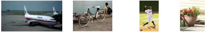
Figure 1: Images from the VisDA-17 domain adaptation challenge
图 1: VisDA-17领域自适应挑战赛中的图像
Recent work [29] has demonstrated the effectiveness of self-ensembling with random image augmentations to achieve state of the art performance in semisupervised learning benchmarks.
近期研究[29]表明,通过随机图像增强实现的自集成(self-ensembling)方法在半监督学习基准测试中取得了最先进的性能。
We have developed the approach proposed by Tarvainen et al. [29] to work in a domain adaptation scenario. We will show that this can achieve excellent results in specific small image domain adaptation benchmarks. More challenging scenarios, notably MNIST $\rightarrow$ SVHN and the VisDA-17 domain adaptation challenge required further modifications. To this end, we developed confidence threshold ing and class balancing that allowed us to achieve state of the art results in a variety of benchmarks, with some of our results coming close to those achieved by traditional supervised learning. Our approach is sufficiently flexble to be applicable to a variety of network architectures, both randomly initialized and pre-trained.
我们改进了Tarvainen等人[29]提出的方法,使其适用于领域自适应场景。实验表明,该方法在特定的小规模图像领域自适应基准测试中表现出色。针对更具挑战性的场景(如MNIST $\rightarrow$ SVHN转换和VisDA-17领域自适应挑战),我们进一步开发了置信度阈值化和类别平衡技术,使得该方法在多个基准测试中达到业界领先水平,部分结果甚至接近传统监督学习的性能。该方案具有足够的灵活性,可适用于随机初始化和预训练的各种网络架构。
Our paper is organised as follows; in Section 2 we will discuss related work that provides context and forms the basis of our technique; our approach is described in Section 3 with our experiments and results in Section 4; and finally we present our conclusions in Section 5.
本文结构如下:第2节将讨论相关研究工作,为我们的技术提供背景和基础;第3节描述我们的方法,第4节展示实验与结果;最后在第5节给出结论。
2 Related work
2 相关工作
In this section we will cover self-ensembling based semi-supervised methods that form the basis of our approach and domain adaptation techniques to which our work can be compared.
在本节中,我们将介绍基于自集成(self-ensembling)的半监督方法(这是我们方法的基础)以及领域自适应技术(我们的工作可与之进行比较)。
2.1 Self-ensembling for semi-supervised learning
2.1 半监督学习的自集成方法
Recent work based on methods related to self-ensembling have achieved excellent results in semi-supervised learning scenarious. A neural network is trained to make consistent predictions for unsupervised samples under different augmentation [24], dropout and noise conditions or through the use of adversarial training [18]. We will focus in particular on the self-ensembling based approaches of Laine et al. [14] and Tarvainen et al. [29] as they form the basis of our approach.
基于自集成(self-ensembling)相关方法的最新研究在半监督学习场景中取得了优异成果。这类方法通过训练神经网络使其在不同数据增强[24]、dropout、噪声条件下或通过对抗训练[18]对无监督样本做出稳定预测。我们将特别关注Laine等人[14]和Tarvainen等人[29]提出的自集成方法,这些方法构成了本文研究的基础。
Laine et al. [14] present two models; their $\mathrm{II}$ -model and their temporal model. The $\mathrm{II}$ -model passes each unlabeled sample through a classifier twice, each time with different dropout, noise and image translation parameters. Their unsupervised loss is the mean of the squared difference in class probability predictions resulting from the two presentations of each sample. Their temporal model maintains a per-sample moving average of the historical network predictions and encourages subsequent predictions to be consistent with the average. Their approach achieved state of the art results in the SVHN and CIFAR-10 semisupervised classification benchmarks.
Laine等人[14]提出了两种模型:其$\mathrm{II}$模型和时序模型。$\mathrm{II}$模型将每个未标注样本两次输入分类器,每次采用不同的dropout、噪声和图像平移参数。无监督损失函数定义为两次预测所得类别概率的平方差均值。时序模型则维护每个样本历史网络预测的移动平均值,并促使后续预测与该平均值保持一致。该方法在SVHN和CIFAR-10半监督分类基准测试中取得了当时最先进的结果。
Tarvainen et al. [29] further improved on the temporal model [14] by using an exponential moving average of the network weights rather than of the class predictions. Their approach uses two networks; a student network and a teacher network, where the student is trained using gradient descent and the weigthts of the teacher are the exponential moving average of those of the student. The unsupervised loss used to train the student is the mean square difference between the predictions of the student and the teacher, under different dropout, noise and image translation parameters.
Tarvainen等人[29]通过使用网络权重的指数移动平均而非类别预测的指数移动平均,进一步改进了时序模型[14]。他们的方法采用两个网络:学生网络和教师网络,其中学生网络通过梯度下降进行训练,而教师网络的权重是学生网络权重的指数移动平均。用于训练学生网络的无监督损失是在不同dropout、噪声和图像变换参数下,学生网络与教师网络预测之间的均方差。
2.2 Domain adaptation
2.2 领域自适应
There is a rich body of literature tackling the problem of domain adaptation. We focus on deep learning based methods as these are most relevant to our work.
针对领域适应问题已有大量研究文献。我们重点关注基于深度学习的方法,因其与我们的工作最为相关。
Auto-encoders are unsupervised neural network models that reconstruct their input samples by first encoding them into a latent space and then decoding and reconstructing them. Ghifary et al. [6] describe an auto-encoder model that is trained to reconstruct samples from both the source and target domains, while a classifier is trained to predict labels from domain invariant features present in the latent representation using source domain labels. Bousmalis et al. [2] re ck ogni sed that samples from disparate domains have distinct domain specific characteristics that must be represented in the latent representation to support effective reconstruction. They developed a split model that separates the latent representation into shared domain invariant features and private features specific to the source and target domains. Their classifier operates on the domain invariant features only.
自动编码器 (auto-encoder) 是一种无监督神经网络模型,通过先将输入样本编码到潜在空间,再进行解码和重构来重建输入样本。Ghifary 等人 [6] 描述了一种自动编码器模型,该模型经过训练可以同时重建源域和目标域的样本,同时使用源域标签训练分类器从潜在表示中的域不变特征预测标签。Bousmalis 等人 [2] 认识到不同域的样本具有独特的域特定特征,这些特征必须在潜在表示中体现以支持有效重建。他们开发了一种拆分模型,将潜在表示分离为共享的域不变特征以及源域和目标域特有的私有特征。他们的分类器仅基于域不变特征进行操作。
Ganin et al. [5] propose a bifurcated classifier that splits into label classification and domain classification branches after common feature extraction layers. A gradient reversal layer is placed between the common feature extraction layers and the domain classification branch; while the domain classification layers attempt to determine which domain a sample came from the gradient reversal operation encourages the feature extraction layers to confuse the domain classifier by extracting domain invariant features. An alternative and simpler implementation described in their appendix minimises the label cross-entropy loss in the feature and label classification layers, minimises the domain crossentropy in the domain classification layers but maximises it in the feature layers. The model of Tzeng et al. [30] runs along similar lines but uses separate feature extraction sub-networks for source and domain samples and train the model in two distinct stages.
Ganin等人[5]提出了一种分叉分类器,在共享特征提取层后分为标签分类和域分类分支。在共享特征提取层与域分类分支之间设置了梯度反转层:当域分类层试图判断样本来源域时,梯度反转操作会促使特征提取层通过提取域不变特征来混淆域分类器。其附录描述的另一种更简单实现是:在特征层和标签分类层最小化标签交叉熵损失,在域分类层最小化域交叉熵损失,但在特征层最大化该损失。Tzeng等人[30]的模型思路类似,但为源域和目标域样本使用独立特征提取子网络,并分两个不同阶段训练模型。
Saito et al. [22] use tri-training [32]; feature extraction layers are used to drive three classifier sub-networks. The first two are trained on samples from the source domain, while a weight similarity penalty encourages them to learn different weights. Pseudo-labels generated for target domain samples by these source domain class if i ers are used to train the final classifier to operate on the target domain.
Saito等人[22]采用三重训练(tri-training)[32]方法:通过特征提取层驱动三个分类器子网络。前两个子网络在源域样本上进行训练,同时权重相似性惩罚机制促使它们学习不同的权重。由这些源域分类器为目标域样本生成的伪标签(pseudo-labels)被用于训练最终能在目标域上运作的分类器。
Generative Adversarial Networks [7] (GANs) are unsupervised models that consist of a generator network that is trained to generate samples that match the distribution of a dataset by fooling a disc rim in at or network that is simultaneously trained to distinguish real samples from generates samples. Some GAN based models – such as that of Sankara narayan an et al. [25] – use a GAN to help learn a domain invariant embedding for samples. Many GAN based domain adaptation approaches use a generator that transforms samples from one domain to another.
生成对抗网络 [7] (GAN) 是无监督模型,由生成器网络和判别器网络组成。生成器通过欺骗判别器来生成与数据集分布匹配的样本,而判别器则被训练用于区分真实样本与生成样本。部分基于GAN的模型(如Sankaranarayanan等人 [25] 提出的方案)利用GAN来学习样本的领域不变嵌入。许多基于GAN的领域自适应方法采用生成器将样本从一个领域转换到另一个领域。
Bousmalis et al. [1] propose a GAN that adapts synthetic images to better match the characteristics of real images. Their generator takes a synthetic image and noise vector as input and produces an adapted image. They train a classifier to predict annotations for source and adapted samples alonside the GAN, while encouraing the generator to preserve aspects of the image important for annotation. The model of [26] consists of a refiner network (in the place of a generator) and disc rim in at or that have a limited receptive field, limiting their model to making local changes while preserving ground truth annotations. The use of refined simulated images with corresponding ground truths resulted in improved performance in gaze and hand pose estimation.
Bousmalis等人[1]提出了一种生成对抗网络(GAN),用于调整合成图像以更好地匹配真实图像特征。其生成器以合成图像和噪声向量为输入,输出适配后的图像。他们在训练GAN的同时训练分类器来预测源样本和适配样本的标注,并鼓励生成器保留对标注重要的图像特征。[26]的模型包含一个精炼网络(替代生成器)和感受野受限的判别器,使其模型仅能进行局部修改同时保留真实标注。使用带有对应真实标注的精炼仿真图像,在视线和手部姿态估计任务中取得了性能提升。
Russo et al. [21] present a bi-directional GAN composed of two generators that transform samples from the source to the target domain and vice versa. They transform labelled source samples to the target domain using one generator and back to the source domain with the other and encourage the network to learn label class consistency. This work bears similarities to CycleGAN [33].
Russo等[21]提出了一种双向GAN,由两个生成器组成,分别将样本从源域转换到目标域以及反向转换。他们使用一个生成器将带标签的源样本转换到目标域,再用另一个生成器转换回源域,从而促使网络学习标签类别一致性。该工作与CycleGAN[33]有相似之处。
A number of domain adaptation models maximise domain confusion by minimising the difference between the distributions of features extracted from source and target domains. Deep CORAL [28] minimises the difference between the feature covariance matrices for a mini-batch of samples from the source and target domains. Tzeng et al. [31] and Long et al. [17] minimise the Maximum Mean Discrepancy metric [8]. Li et al. [15] described adaptive batch normalization, a variant of batch normalization [12] that learns separate batch normalization statistics for the source and target domains in a two-pass process, establishing new state-of-the-art results. In the first pass standard supervised learning is used to train a classifier for samples from the source domain. In the second pass, normalization statistics for target domain samples are computed for each batch normalization layer in the network, leaving the network weights as they are.
许多领域自适应模型通过最小化从源域和目标域提取的特征分布之间的差异来最大化领域混淆。Deep CORAL [28] 最小化了源域和目标域小批量样本特征协方差矩阵之间的差异。Tzeng等人 [31] 和Long等人 [17] 最小化了最大均值差异度量 [8]。Li等人 [15] 提出了自适应批量归一化 (adaptive batch normalization),这是批量归一化 [12] 的一种变体,通过两阶段过程学习源域和目标域各自的批量归一化统计量,从而取得了新的最先进成果。第一阶段使用标准监督学习训练源域样本的分类器。第二阶段为网络中的每个批量归一化层计算目标域样本的归一化统计量,同时保持网络权重不变。
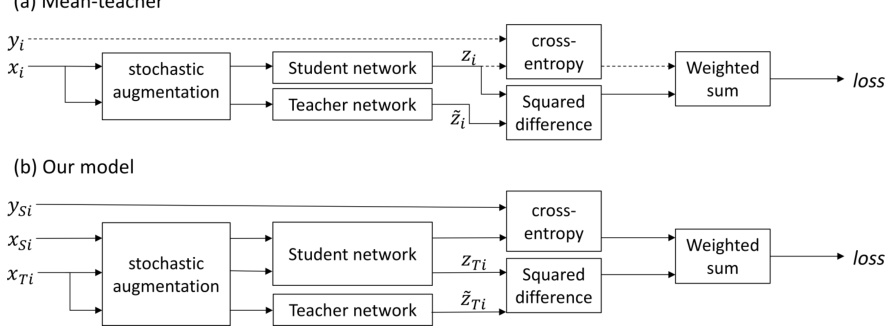
Figure 2: The network structures of the original mean teacher model and our model. Dashed lines in the mean teacher model indicate that ground truth labels – and therefore cross-entropy classification loss – are only available for labeled samples.
图 2: 原始均值教师模型与我们提出的模型网络结构对比。均值教师模型中的虚线表示真实标签(及对应的交叉熵分类损失)仅适用于已标注样本。
3 Method
3 方法
Our model builds upon the mean teacher semi-supervised learning model [29], which we will describe. Subsequently we will present our modifications that enable domain adaptation.
我们的模型基于均值教师半监督学习模型 [29],接下来将对其进行描述。随后我们将介绍实现领域自适应的改进部分。
The structure of the mean teacher model [29] – also discussed in section 2.1 – is shown in Figure 2a. The student network is trained using gradient descent, while the weights of the teacher network are an exponential moving average of those of the student. During training each input sample $x_{i}$ is passed through both the student and teacher networks, generating predicted class probability vectors $z_{i}$ (student) and $\tilde{z}_{i}$ (teacher). Different dropout, noise and image translation parameters are used for the student and teacher pathways.
均值教师模型 [29] 的结构(2.1 节亦有讨论)如图 2a 所示。学生网络通过梯度下降进行训练,教师网络的权重则是学生网络权重的指数移动平均值。训练过程中每个输入样本 $x_{i}$ 会同时通过学生网络和教师网络,分别生成预测类别概率向量 $z_{i}$(学生网络)和 $\tilde{z}_{i}$(教师网络)。学生网络与教师网络采用不同的 dropout、噪声和图像平移参数。
During each training iteration a mini-batch of samples is drawn from the dataset, consisting of both labeled and unlabeled samples. The training loss is the sum of a supervised and an unsupervised component. The supervised loss is cross-entropy loss computed using $z_{i}$ (student prediction). It is masked to $0$ for unlabeled samples for which no ground truth is available. The unsupervised component is the self-ensembling loss. It penalises the difference in class predictions between student ( $z_{i}$ ) and teacher $(\Tilde{z}{i})$ networks for the same input sample. It is computed using the mean squared difference between the class probability predictions $z_{i}$ and $\tilde{z}_{i}$ .
在每次训练迭代中,会从数据集中抽取一个小批量样本,包含已标注和未标注样本。训练损失由监督损失和无监督损失两部分组成。监督损失是使用学生网络预测$z_{i}$计算的交叉熵损失,对于没有真实标签的未标注样本会将该损失掩码为$0$。无监督部分是自集成损失,它惩罚同一输入样本在学生网络($z_{i}$)和教师网络$(\Tilde{z}{i})$之间的类别预测差异,通过计算类别概率预测$z_{i}$与$\tilde{z}_{i}$之间的均方差来实现。
Laine et al. [14] and Tarvainen et al. [29] found that it was necessary to apply a time-dependent weighting to the unsupervised loss during training in order to prevent the network from getting stuck in a degenerate solution that gives poor classification performance. They used a function that follows a Gaussian curve from 0 to 1 during the first 80 epochs.
Laine等人[14]和Tarvainen等人[29]发现,在训练过程中需要对无监督损失施加时间依赖性权重,以防止网络陷入导致分类性能下降的退化解。他们采用了一个在前80个训练周期内遵循从0到1高斯曲线的函数。
In the following subsections we will describe our contributions in detail along with the motivations for introducing them.
在接下来的小节中,我们将详细描述我们的贡献以及引入这些贡献的动机。
3.1 Adapting to domain adaptation
3.1 适应领域自适应
We minimise the same loss as in [29]; we apply cross-entropy loss to labeled source samples and unsupervised self-ensembling loss to target samples. As in [29], self-ensembling loss is computed as the mean-squared difference between predictions produced by the student $\left(z_{T i}\right)$ and teacher $\left(\tilde{z}_{T i}\right)$ networks with different augmentation, dropout and noise parameters.
我们采用与[29]相同的损失函数:对带标签的源样本应用交叉熵损失,对目标样本应用无监督自集成损失。如[29]所述,自集成损失通过计算学生网络$\left(z_{T i}\right)$和教师网络$\left(\tilde{z}_{T i}\right)$在不同增强、dropout及噪声参数下生成预测的均方差得到。
The models of [29] and of [14] were designed for semi-supervised learning problems in which a subset of the samples in a single dataset have ground truth labels. During training both models mix labeled and unlabeled samples together in a mini-batch. In contrast, unsupervised domain adaptation problems use two distinct datasets with different underlying distributions; labeled source and unlabeled target. Our variant of the mean teacher model – shown in Figure 2b – has separate source $(X_{S i})$ and target $(X_{T i,}$ ) paths. Inspired by [15], we process mini-batches from the source and target datasets separately (per iteration) so that batch normalization uses different normalization statistics for each domain during training.1. We do not use the approach of [15] as-is, as they handle the source and target datasets separtely in two distinct training phases, where our approach must train using both simultaneously. We also do not maintain separate exponential moving averages of the means and variances for each dataset for use at test time.
[29]和[14]的模型专为半监督学习问题设计,这类问题中单个数据集的部分样本带有真实标签。训练时,两种模型都将带标签和无标签样本混合在小批量(mini-batch)中处理。相比之下,无监督领域自适应问题使用两个具有不同底层分布的数据集:带标签的源域和无标签的目标域。我们对均值教师模型的改进版本(如图2b所示)设有独立的源域$(X_{S i})$和目标域$(X_{T i,}$)处理路径。受[15]启发,我们在每次迭代中分别处理源域和目标域的小批量数据,使得批量归一化(batch normalization)在训练期间能为每个领域使用不同的归一化统计量。
- 我们没有直接采用[15]的方法,因为他们的方案在两个独立训练阶段分别处理源域和目标域数据,而我们的方法需要同时使用两者进行训练。我们也没有为测试阶段维护各数据集均值与方差的独立指数移动平均值。
As seen in the ‘MT $^+$ TF’ row of Table 1, the model described thus far achieves state of the art results in 5 out of 8 small image benchmarks. The MNIST $\rightarrow$ SVHN, STL $\rightarrow$ CIFAR-10 and Syn-digits $\rightarrow$ SVHN benchmarks however require additional modifications to achieve good performance.
如表 1 中 "MT $^+$ TF" 行所示,目前描述的模型在 8 个小型图像基准测试中有 5 项达到了最先进水平。然而,MNIST $\rightarrow$ SVHN、STL $\rightarrow$ CIFAR-10 和 Syn-digits $\rightarrow$ SVHN 基准测试需要进行额外修改才能获得良好性能。
3.2 Confidence threshold ing
3.2 置信度阈值处理
We found that replacing the Gaussian ramp-up factor that scales the unsupervised loss with confidence threshold ing stabilized training in more challenging domain adaptation scenarios. For each unlabeled sample $x T i$ the teacher network produces the predicted class probabilty vector $\tilde{z}{T i j}$ – where $j$ is the class index drawn from the set of classes $C$ – from which we compute the confidence $\tilde{f}{T i}=\mathrm{max}{j\in C}(\tilde{z}{T i j})$ ; the predicted probability of the predicted class of the sample. If $\tilde{f}{T i}$ is below the confidence threshold (a parameter search found 0.968 to be an effective value for small image benchmarks), the self-ensembling loss for the sample $x_{i}$ is masked to $0$ .
我们发现,在更具挑战性的领域自适应场景中,用置信度阈值替换用于缩放无监督损失的高斯斜坡因子可以稳定训练。对于每个未标记样本$x T i$,教师网络生成预测的类别概率向量$\tilde{z}{T i j}$(其中$j$是从类别集$C$中抽取的类别索引),由此计算置信度$\tilde{f}{T i}=\mathrm{max}{j\in C}(\tilde{z}{T i j})$(即样本预测类别的概率)。若$\tilde{f}{T i}$低于置信度阈值(参数搜索发现0.968对小图像基准测试有效),则样本$x_{i}$的自集成损失被掩码为$0$。
Our working hypothesis is that confidence threshold ing acts as a filter, shifting the balance in favour of the student learning correct labels from the teacher. While high network prediction confidence does not guarantee correctness there is a positive correlation. Given the tolerance to incorrect labels reported in [14], we believe that the higher signal-to-noise ratio underlies the success of this component of our approach.
我们的工作假设是,置信度阈值起到了过滤器的作用,使天平向学生从教师那里学习正确标签倾斜。虽然网络预测的高置信度并不能保证正确性,但两者存在正相关性。鉴于[14]中报告的对错误标签的容忍度,我们认为更高的信噪比是我们方法这一部分成功的基础。
The use of confidence threshold ing achieves a state of the art results in the STL $\rightarrow$ CIFAR-10 and Syn-digits $\rightarrow$ SVHN benchmarks, as seen in the ‘MT $^+$ CT $^+$ TF’ row of Table 1. While confidence threshold ing can result in very slight reductions in performance (see the MNIST $\leftrightarrow$ USPS and SVHN MNIST results), its ability to stabilise training in challenging scenarios leads us to recommend it as a replacement for the time-dependent Gaussian ramp-up used in [14].
在STL $\rightarrow$ CIFAR-10和Syn-digits $\rightarrow$ SVHN基准测试中,置信度阈值(confidence thresholding)的应用达到了最先进水平,如表1中"MT$^+$CT$^+$TF"行所示。虽然置信度阈值可能导致性能略微下降(参见MNIST $\leftrightarrow$ USPS和SVHN $\rightarrow$ MNIST结果),但其在具有挑战性的场景中稳定训练的能力,使我们推荐用它替代[14]中使用的随时间变化的高斯斜坡上升方法。
3.3 Data augmentation
3.3 数据增强
We explored the effect of three data augmentation schemes in our small image benchmarks (section 4.1). Our minimal scheme (that should be applicable in non-visual domains) consists of Gaussian noise (with $\sigma=0.1$ ) added to the pixel values. The standard scheme (indicated by ‘TF’ in Table 1) was used in [14] and adds translations in the interval $[-2,2]$ and horizontal flips for the CIFAR $10\leftrightarrow$ STL experiments. The affine scheme (indicated by ‘TFA’) adds random affine transformations defined by the matrix in (1), where $\mathcal{N}(0,0.1)$ denotes a real value drawn from a normal distribution with mean $0$ and standard deviation 0.1.
我们在小型图像基准测试(4.1节)中探索了三种数据增强方案的效果。我们的基础方案(适用于非视觉领域)包含向像素值添加高斯噪声(σ=0.1)。标准方案(表1中标注为"TF")采用文献[14]的方法,在CIFAR10↔STL实验中添加[-2,2]区间内的平移和水平翻转。仿射方案(标注为"TFA")则添加了由矩阵(1)定义的随机仿射变换,其中N(0,0.1)表示从均值为0、标准差为0.1的正态分布中抽取的实数值。
$$
\begin{array}{r}{\left[1+\mathcal{N}(0,0.1)\quad\quad\mathcal{N}(0,0.1)\right]}\ {\mathcal{N}(0,0.1)\quad\quad1+\mathcal{N}(0,0.1)}\end{array}
$$
$$
\begin{array}{r}{\left[1+\mathcal{N}(0,0.1)\quad\quad\mathcal{N}(0,0.1)\right]}\ {\mathcal{N}(0,0.1)\quad\quad1+\mathcal{N}(0,0.1)}\end{array}
$$
The use of translations and horizontal flips has a significant impact in a number of our benchmarks. It is necessary in order to outpace prior art in the MNIST $\leftrightarrow$ USPS and SVHN $\rightarrow$ MNIST benchmarks and improves performance in the CIFAR $10\leftrightarrow\mathrm{STL}$ benchmarks. The use of affine augmentation can improve performance in experiments involving digit and traffic sign recognition datasets, as seen in the ‘MT $^+$ CT+TFA’ row of Table 1. In contrast it can impair performance when used with photographic datasets, as seen in the the STL $\rightarrow$ CIFAR-10 experiment. It also impaired performance in the VisDA-17 experiment (section 4.2).
翻译和水平翻转的使用在我们的多项基准测试中产生了显著影响。为了在MNIST $\leftrightarrow$ USPS和SVHN $\rightarrow$ MNIST基准测试中超越现有技术,这一操作是必要的,同时也在CIFAR $10\leftrightarrow\mathrm{STL}$ 基准测试中提升了性能。仿射增强的使用可以提高涉及数字和交通标志识别数据集的实验性能,如表1中"MT $^+$ CT+TFA"行所示。相反,当用于摄影数据集时,它可能会损害性能,如STL $\rightarrow$ CIFAR-10实验所示。在VisDA-17实验(章节4.2)中,它同样降低了性能。
3.4 Class balance loss
3.4 类别平衡损失
With the adaptations made so far the challenging MNIST $\rightarrow$ SVHN benchmark remains undefeated due to training instabilities. During training we noticed that the error rate on the SVHN test set decreases at first, then rises and reaches high values before training completes. We diagnosed the problem by recording the predictions for the SVHN target domain samples after each epoch. The rise in error rate correlated with the predictions evolving toward a condition in which most samples are predicted as belonging to the ‘1’ class; the most populous class in the SVHN dataset. We hypothesize that the class imbalance in the SVHN dataset caused the unsupervised loss to reinforce the ‘1’ class more often than the others, resulting in the network settling in a degenerate local minimum. Rather than distinguish between digit classes as intended it seperated MNIST from SVHN samples and assigned the latter to the ‘1’ class.
经过前述调整后,由于训练不稳定性,具有挑战性的MNIST $\rightarrow$ SVHN基准测试仍未取得突破。训练过程中我们观察到:SVHN测试集的错误率初期下降,随后回升并在训练结束前达到峰值。通过记录每轮迭代后SVHN目标域样本的预测结果,我们发现问题症结在于错误率上升与预测结果逐渐偏向"1"类相关(该类别在SVHN数据集中样本量最大)。我们推测SVHN数据集的类别不平衡性导致无监督损失更频繁地强化"1"类,使网络陷入退化的局部最小值——模型未能按预期区分数字类别,而是将MNIST与SVHN样本分离并将后者全部归类为"1"。
We addressed this problem by introducing a class balance loss term that penalises the network for making predictions that exhibit large class imbalance. For each target domain mini-batch we compute the mean of the predicted sample class probabilities over the sample dimension, resulting in the mini-batch mean per-class probability. The loss is computed as the binary cross entropy between the mean class probability vector and a uniform probability vector. We balance the strength of the class balance loss with that of the self-ensembling loss by multiplying the class balance loss by the average of the confidence threshold mask (e.g. if 75% of samples in a mini-batch pass the confidence threshold, then the class balance loss is multiplied by 0.75).2
我们通过引入一个类别平衡损失项来解决这个问题,该损失项会对网络预测中出现较大类别不平衡的情况进行惩罚。对于每个目标域的小批量数据,我们计算样本维度上预测样本类别概率的均值,得到小批量数据的每类平均概率。该损失计算为平均类别概率向量与均匀概率向量之间的二元交叉熵。我们通过将类别平衡损失乘以置信度阈值掩码的平均值(例如,如果小批量中75%的样本通过置信度阈值,则类别平衡损失乘以0.75),来平衡类别平衡损失与自集成损失的强度。
We would like to note the similarity between our class balance loss and the entropy maxim is ation loss in the IMSAT clustering model of Hu et al. [11]; IMSAT employs entropy maxim is ation to encourage uniform cluster sizes and entropy minim is ation to encourage unambiguous cluster assignments.
我们想指出,我们的类别平衡损失与Hu等人[11]的IMSAT聚类模型中的熵最大化损失有相似之处;IMSAT采用熵最大化来促进均匀的簇大小,采用熵最小化来促进明确的簇分配。
4 Experiments
4 实验
Our implementation was developed using PyTorch ([3]) and is publically available at http://github.com/Britefury/self-ensemble-visual-domain-adapt
我们的实现基于PyTorch语言([3])开发,代码已开源在http://github.com/Britefury/self-ensemble-visual-domain-adapt
4.1 Small image datasets
4.1 小型图像数据集
Our results can be seen in Table 1. The ‘train on source’ and ‘train on target’ results report the target domain performance of supervised training on the source and target domains. They represent the exepected baseline and best achievable result. The ‘Specific aug.‘ experiments used data augmentation specific to the MNIST $\rightarrow$ SVHN adaptation path that is discussed further down.
我们的结果如表1所示。"在源域训练"和"在目标域训练"的结果分别报告了在源域和目标域进行监督训练的目标域性能。它们代表了预期的基线水平和可达到的最佳结果。"特定增强"实验使用了针对MNIST→SVHN适配路径的特定数据增强方法,具体讨论见下文。
The small datasets and data preparation procedures are described in Appendix A. Our training procedure is described in Appendix B and our network architectures are described in Appendix D. The same network architectures and augmentation parameters were used for domain adaptation experiments and the supervised baselines discussed above. It is worth noting that only the training sets of the small image datasets were used during training; the test sets used for reporting scores only.
小规模数据集和数据准备流程详见附录A。训练流程见附录B,网络架构详见附录D。域适应实验和上述监督基线均采用相同网络架构与数据增强参数。需注意的是,训练阶段仅使用小规模图像数据集的训练集,测试集仅用于分数报告。
MNIST $\leftrightarrow$ USPS (see Figure 3a). MNIST and USPS are both greyscale hand-written digit datasets. In both adaptation directions our approach not only demonstrates a significant improvement over prior art but nearly achieves the performance of supervised learning using the target domain ground truths. The strong performance of the base mean teacher model can be attributed to the similarity of the datasets to one another. It is worth noting that data augmentation allows our ‘train on source’ baseline to outpace prior domain adaptation methods.
MNIST $\leftrightarrow$ USPS (见图 3a)。MNIST 和 USPS 都是灰度手写数字数据集。在这两个适应方向上,我们的方法不仅显著优于现有技术,而且几乎达到了使用目标域真实标签进行监督学习的性能。基础均值教师模型的强大性能可归因于数据集之间的相似性。值得注意的是,数据增强使我们的"在源域训练"基线超越了先前的域适应方法。
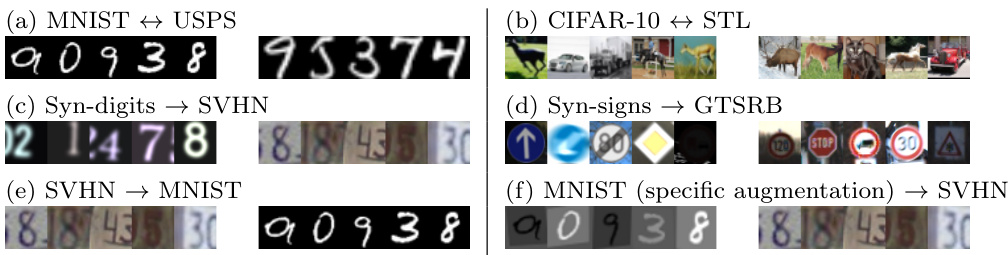
Figure 3: Small image domain adaptation example images
图 3: 小图像域适应示例图像
CIFAR-10 ↔ STL (see Figure 3b). CIFAR-10 and STL are both 10-class image datasets, although we removed one class from each (see Appendix A.2). We obtained strong performance in the STL $\rightarrow$ CIFAR-10 path, but only by using confidence threshold ing. The CIFAR $10\rightarrow$ STL results are more interesting; the ‘train on source’ baseline performance outperforms that of a network trained on the STL target domain, most likely due to the small size of the STL training set. Our self-ensembling results outpace both the baseline performance and the ‘theoretical maximum’ of a network trained on the target domain, lending further evidence to the view of [24] and [14] that self-ensembling acts as an effective regular is er.
CIFAR-10 ↔ STL (见图 3b)。CIFAR-10 和 STL 都是 10 类图像数据集,尽管我们从中各移除了一类 (见附录 A.2)。我们在 STL → CIFAR-10 路径上取得了强劲性能,但仅在使用置信度阈值时实现。CIFAR-10 → STL 的结果更有趣:"在源域训练"的基线性能超过了在 STL 目标域训练的网络,这很可能是由于 STL 训练集规模较小。我们的自集成 (self-ensembling) 结果超越了基线性能和在目标域训练网络的"理论最大值",这进一步佐证了 [24] 和 [14] 的观点:自集成可作为一种有效的正则化器。
Syn-Digits $\rightarrow$ SVHN (see Figure 3c). The Syn-Digits dataset is a synthetic dataset designed by [5] to be used as a source dataset in domain adaptation experiments with SVHN as the target dataset. Other approaches have achieved good scores on this benchmark, beating the baseline by a significant margin. Our result improves on them, reducing the error rate from 6.9% to $2.9%$ ; even slightly outpacing the ‘train on target’ 3.4% error rate achieved using supervised learning.
Syn-Digits $\rightarrow$ SVHN (见图 3c)。Syn-Digits 数据集是由 [5] 设计的合成数据集,旨在作为域适应实验中的源数据集,并以 SVHN 作为目标数据集。其他方法在该基准测试中取得了不错的成绩,显著超越了基线水平。我们的结果进一步优化了这些方法,将错误率从 6.9% 降至 $2.9%$,甚至略微优于使用监督学习在目标数据集上训练得到的 3.4% 错误率。
Syn-Signs $\rightarrow$ GTSRB (see Figure 3d). Syn-Signs is another synthetic dataset designed by [5] to target the 43-class GTSRB [27] (German Traffic Signs Recognition Benchmark) dataset. Our approach halved the best error rate of competing approaches. Once again, our approaches slightly outpaces the ‘train on target’ supervised learning upper bound.
Syn-Signs $\rightarrow$ GTSRB (见图 3d)。Syn-Signs 是 [5] 为针对 43 类 GTSRB [27] (German Traffic Signs Recognition Benchmark) 数据集设计的另一个合成数据集。我们的方法将竞争方法的最佳错误率降低了一半。此外,我们的方法再次略微超越了"在目标数据上训练"的监督学习上限。
SVHN $\rightarrow$ MNIST (see Figure 3e). Google’s SVHN (Street View House Numbers) is a colour digits dataset of house number plates. Our approach significantly outpaces other techniques and achieves an accuracy close to that of supervised learning.
SVHN $\rightarrow$ MNIST (见图 3e)。Google 的 SVHN (Street View House Numbers) 是一个包含门牌号码的彩色数字数据集。我们的方法显著优于其他技术,并达到了接近监督学习的准确率。
MNIST $\rightarrow$ SVHN (see Figure 3f). This adaptation path is somewhat more challenging as MNIST digits are greyscale and uniform in terms of size, aspect ratio and intensity range, in contrast to the variably sized colour digits present in SVHN. As a consequence, adapting from MNIST to SVHN required additional work. Class balancing loss was necessary to ensure training stability and additional experiment specific data augmentation was required to achieve good accuracy. The use of translations and affine augmentation (see section 3.3) results in an accuracy score of 37%. Significant improvements resulted from additional augmentation in the form of random intensity flips (negative image), and random intensity scales and offsets drawn from the intervals [0.25, 1.5] and $[-0.5,0.5]$ respectively. These hyper-parameters were selected in order to augment MNIST samples to match the intensity variations present in SVHN, as illustrated in Figure 3f. With these additional modifications, we achieve a result that significantly outperforms prior art and nearly achieves the accuracy of a supervised classifier trained on the target dataset. We found that applying these additional augmentations to the source MNIST dataset only yielded good results; applying them to the target SVHN dataset as well yielded a small improvement but was not essential. It should also be noted that this augmentation scheme raises the performance of the ‘train on source’ baseline to just above that of much of the prior art.
MNIST $\rightarrow$ SVHN (见图 3f)。这一适应路径更具挑战性,因为MNIST数字是灰度图像且尺寸、长宽比和强度范围统一,而SVHN中的彩色数字存在尺寸变化。因此,从MNIST适应到SVHN需要额外工作:必须使用类别平衡损失确保训练稳定性,并增加实验专用的数据增强以获得良好准确率。采用平移和仿射增强 (见3.3节) 可使准确率达到37%。通过随机强度翻转 (负片效果) 以及从区间[0.25, 1.5]和$[-0.5,0.5]$分别抽取的随机强度缩放与偏移进行增强后,性能显著提升。选择这些超参数是为了增强MNIST样本以匹配SVHN的强度变化 (如图3f所示)。经过这些额外改进,我们的结果显著优于现有技术,几乎达到在目标数据集上训练的有监督分类器的准确率。值得注意的是,仅对源MNIST数据集应用这些增强即可获得良好效果,虽对目标SVHN数据集同步增强能带来小幅提升但非必需。该增强方案还将"在源数据训练"基线的性能提升至超越多数现有技术的水平。
4.2 VisDA-2017 visual domain adaptation challenge
4.2 VisDA-2017视觉域自适应挑战赛
The VisDA-2017 image classification challenge is a 12-class domain adaptation problem consisting of three datasets: a training set consisting of 3D renderings of sketchup models, and validation and test sets consisting of real images (see Figure 1) drawn from the COCO [16] and YouTube Bounding Boxes [20] datasets respectively. The objective is to learn from labeled computer generated images and correctly predict the class of real images. Ground truth labels were made available for the training and validation sets only; test set scores were computed by a server operated by the competition organisers.
VisDA-2017图像分类挑战赛是一个包含12个类别的域适应问题,由三个数据集组成:训练集包含SketchUp模型的三维渲染图,验证集和测试集则分别包含来自COCO [16] 和YouTube Bounding Boxes [20] 数据集的真实图像(见图1)。该挑战的目标是从带标签的计算机生成图像中学习,并正确预测真实图像的类别。训练集和验证集提供了真实标签;测试集得分由竞赛组织者运营的服务器计算得出。
While the algorithm is that presented above, we base our network on the pretrained ResNet-152 [10] network provided by PyTorch ([3]), rather than using a randomly initial is ed network as before. The final 1000-class classification layer is removed and replaced with two fully-connected layers; the first has 512 units with a ReLU non-linearity while the final layer has 12 units with a softmax non-linearity. Results from our original competition submissions and newer results using two data augmentation schemes are presented in Table 2. Our reduced augmentation scheme consists of random crops, random horizontal flips and random uniform scaling. It is very similar to scheme used for ImageNet image classification in [10]. Our competition configuration includes additional augmentation that was specifically designed for the VisDA dataset, although we subsequently found that it makes little difference. Our hyper-parameters and competition data augmentation scheme are described in Appendix C.1. It is worth noting that we applied test time augmentation (we averaged predictions form 16 differently augmented images) to achieve our competition results. We present resuts with and without test time augmentation in Table 2. Our VisDA competition test set score is also the result of ensembling the predictions of 5 different networks.
虽然算法如上所述,但我们基于PyTorch ([3]) 提供的预训练ResNet-152 [10]网络构建模型,而非此前使用的随机初始化网络。移除了最后的1000类分类层,替换为两个全连接层:第一层含512个单元并采用ReLU非线性激活,最后一层含12个单元并采用softmax非线性激活。表2展示了我们原始竞赛提交结果及采用两种数据增强方案的新结果。简化版增强方案包含随机裁剪、随机水平翻转和随机均匀缩放,与[10]中ImageNet图像分类方案高度相似。竞赛配置额外增加了专为VisDA数据集设计的增强方案,但后续发现其影响甚微。超参数及竞赛数据增强方案详见附录C.1。值得注意的是,我们通过测试时增强(对16张不同增强图像的预测取平均)获得竞赛成绩,表2同时展示了采用与未采用测试时增强的结果。VisDA竞赛测试集分数还融合了5个不同网络的预测结果。
5 Conclusions
5 结论
We have presented an effective domain adaptation algorithm that has achieved state of the art results in a number of benchmarks and has achieved accuracies that are almost on par with traditional supervised learning on digit recognition benchmarks targeting the MNIST and SVHN datasets. The resulting networks will exhibit strong performance on samples from both the source and target domains. Our approach is sufficiently flexible to be usable for a variety of network architectures, including those based on randomly initial is ed and pretrained networks.
我们提出了一种高效的领域自适应算法,该算法在多个基准测试中取得了最先进的结果,并在针对MNIST和SVHN数据集的手写数字识别基准测试中达到了与传统监督学习几乎相当的准确率。所得网络在源域和目标域样本上均表现出强劲性能。我们的方法具有足够的灵活性,可适用于各种网络架构,包括基于随机初始化和预训练网络的架构。
Miyato et al. [18] stated that the self-ensembling methods of [14] – on which our algorithm is based – operate by label propagation. This view is supported by our results, in particular our MNIST $\rightarrow$ SVHN experiment. The latter requires additional intensity augmentation in order to sufficiently align the dataset distributions, after which good quality label predictions are propagated throughout the target dataset. In cases where data augmentation is insufficient to align the dataset distributions, a pre-trained network may be used to bridge the gap, as in our solution to the VisDA-17 challenge. This leads us to conclude that effective domain adaptation can be achieved by first aligning the distributions of the source and target datasets – the focus of much prior art in the field – and then refining their correspond ance; a task to which self-ensembling is well suited.
Miyato等人[18]指出,我们算法所基于的[14]自集成方法通过标签传播运作。这一观点得到了我们实验结果的支撑,特别是在MNIST $\rightarrow$ SVHN实验中。后者需要通过额外的强度增强来充分对齐数据集分布,之后高质量的标签预测会在整个目标数据集中传播。当数据增强不足以对齐数据集分布时,可采用预训练网络来弥合差距,如我们在VisDA-17挑战中的解决方案所示。由此我们得出结论:有效的领域自适应可通过先对齐源数据集与目标数据集的分布(该领域许多先前工作的重点),再细化其对应关系来实现——这正是自集成方法特别适合的任务。
Acknowledgments
致谢
This research was funded by a grant from Marine Scotland.
本研究由苏格兰海洋局资助。
We would also like to thank nVidia corporation for their generous donation of a Titan X GPU.
我们还要感谢nVidia公司慷慨捐赠的Titan X GPU。
References
参考文献
A Datasets and Data Preparation
数据集与数据准备
A.1 Small image datasets
A.1 小型图像数据集
The datasets used in this paper are described in Table 3.
本文使用的数据集如表 3 所示。
A.2 Data preparation
A.2 数据准备
Some of the experiments that involved datasets described in Table 3 required additional data preparation in order to match the resolution and format of the input samples and match the classification target. These additional steps will now be described.
表3中涉及的部分实验数据集需要进行额外的数据准备工作,以确保输入样本的分辨率和格式一致,并匹配分类目标。现将这些额外步骤说明如下。
MNIST $\leftrightarrow$ USPS The USPS images were up-scaled using bilinear interpolation from $16\times16$ to $28\times28$ resolution to match that of MNIST.
MNIST $\leftrightarrow$ USPS USPS图像通过双线性插值从$16\times16$分辨率上采样至$28\times28$以匹配MNIST尺寸。
CIFAR $\mathbf{10}\leftrightarrow$ STL CIFAR-10 and STL are both 10-class image datasets. The STL images were down-scaled to $32\times32$ resolution to match that of CIFAR10. The ‘frog’ class in CIFAR-10 and the ‘monkey’ class in STL were removed as they have no equivalent in the other dataset, resulting in a 9-class problem with $10%$ less samples in each dataset.
CIFAR $\mathbf{10}\leftrightarrow$ STL
CIFAR-10和STL均为10类图像数据集。STL图像被降采样至$32\times32$分辨率以匹配CIFAR-10。由于CIFAR-10的"青蛙"类与STL的"猴子"类在对方数据集中无对应类别,这两类被移除,最终形成每个数据集样本量减少$10%$的9分类问题。
Syn-Signs $\rightarrow$ GTSRB GTSRB is composed of images that vary in size and come with annotations that provide region of interest (bounding box around the sign) and ground truth classification. We extracted the region of interest from each image and scaled them to a resolution of $40\times40$ to match those of SynSigns.
Syn-Signs $\rightarrow$ GTSRB
GTSRB由尺寸各异的图像组成,并附带有标注信息,包括感兴趣区域(标志周围的边界框)和真实分类。我们从每张图像中提取感兴趣区域,并将其缩放至$40\times40$分辨率以匹配SynSigns的规格。
MNIST $\leftrightarrow$ SVHN The MNIST images were padded to $32\times32$ resolution and converted to RGB by replicating the greyscale channel into the three RGB channels to match the format of SVHN.
MNIST $\leftrightarrow$ SVHN
MNIST图像被填充至$32\times32$分辨率,并通过将灰度通道复制到RGB三通道转换为RGB格式,以匹配SVHN的数据格式。
B Small image experiment training
B 小图像实验训练
B.1 Training procedure
B.1 训练流程
Our networks were trained for 300 epochs. We used the Adam [13] gradient descent algorithm with a learning rate of 0.001. We trained using mini-batches composed of 256 samples, except in the Syn-digits $\rightarrow$ SVHN and Syn-signs $\rightarrow$ GTSRB experiments where we used 128 in order to reduce memory usage. The self-ensembling loss was weighted by a factor of 3 and the class balancing loss was weighted by 0.005. Our teacher network weights $t_{i}$ were updated so as to be an exponential moving average of those of the student $s_{i}$ using the formula $t_{i}=\alpha t_{i-1}+(1-\alpha)s_{i}$ , with a value of 0.99 for $\alpha$ . A complete pass over the target dataset was considered to be one epoch in all experiments except the MNIST $\rightarrow$ USPS and CIFAR $10\rightarrow$ STL experiments due to the small size of the target datasets, in which case one epoch was considered to be a pass over the larger soure dataset.
我们的网络训练了300个周期。我们使用Adam [13]梯度下降算法,学习率设为0.001。除Syn-digits $\rightarrow$ SVHN和Syn-signs $\rightarrow$ GTSRB实验为降低内存消耗采用128样本的小批量外,其余实验均采用256样本的小批量训练。自集成(self-ensembling)损失的权重系数为3,类别平衡(class balancing)损失的权重系数为0.005。教师网络权重$t_{i}$通过公式$t_{i}=\alpha t_{i-1}+(1-\alpha)s_{i}$更新为学生网络权重$s_{i}$的指数移动平均值,其中$\alpha$取值为0.99。除MNIST $\rightarrow$ USPS和CIFAR $10\rightarrow$ STL实验因目标数据集较小将完整遍历较大源数据集视为一个周期外,其余实验均将完整遍历目标数据集视为一个周期。
We found that using the proportion of samples that passed the confidence threshold can be used to drive early stopping ([19]). The final score was the target test set performance at the epoch at which the highest confidence threshold pass rate was obtained.
我们发现,利用通过置信度阈值的样本比例可以驱动早停机制 ([19])。最终得分是在获得最高置信度阈值通过率的训练轮次时,目标测试集上的性能表现。
C VisDA-17
C VisDA-17
C.1 Hyper-parameters
C.1 超参数
Our training procedure was the same as that used in the small image experiments, except that we used $160\times160$ images, a batch size of 56 (reduced from 64 to fit within the memory of an nVidia 1080-Ti), a self-ensembling weight of 10 (instead of 3), a confidence threshold of 0.9 (instead of 0.968) and a class balancing weight of 0.01. We used the Adam [13] gradient descent algorithm with a learning rate of $10^{-5}$ for the final two randomly initialized layers and $10^{-6}$ for the pre-trained layers. The first convolutional layer and the first group of convolutional layers (with 64 feature channels) of the pre-trained ResNet were left unmodified during training.
我们的训练流程与小图像实验相同,只是使用了160×160尺寸的图像、批量大小为56(从64降低以适应nVidia 1080-Ti显存)、自集成权重为10(原为3)、置信度阈值为0.9(原为0.968)以及类别平衡权重0.01。我们采用Adam [13]梯度下降算法,最后两个随机初始化层的学习率为10⁻⁵,预训练层为10⁻⁶。预训练ResNet的首个卷积层及首组卷积层(含64个特征通道)在训练期间保持冻结。
Reduced data augmentation:
减少数据增强:
Competition data augmentation adds the following in addition to the above:
竞赛数据增强在以上基础上额外增加了:
D Network architectures
D 网络架构
Our network architectures are shown in Tables 6 - 8.
我们的网络架构如表 6 - 8 所示。
[1] [5], [2] [6], [3] [25], [4] [30], [5] [22], [6] [21], [7] [9] a RevGrad results were available in both [5] and [6]; we drew results from both papers to obtain results for all of the experiments shown. b MNIST $\rightarrow$ SVHN specific intensity augmentation as described in Section 4.1. c MNIST $\rightarrow$ SVHN experiments used class balance loss.
| USPS | MNIST | SVHN | MNIST | CIFAR | STL | Syn Digits | Syn Signs | |
|---|---|---|---|---|---|---|---|---|
| MNIST | USPS | MNIST | SVHN | STL | CIFAR | GTSRB | ||
| 在源数据上训练 | ||||||||
| SupSrc* | 77.55 ±0.8 | 82.03 ±1.16 | 66.5 ±1.93 68.65 | 25.44 ±2.8 24.86 | 72.84 ±0.61 | 51.88 ±1.44 | 86.86 ±0.86 | 96.95 ±0.36 |
| SupSrc+TF | 77.53 ±4.63 | 95.39 ±0.93 | ±1.5 | ±3.29 | 75.2 ±0.28 | 59.06 ±1.02 | 87.45 ±0.65 | 97.3 ±0.16 |
| SupSrc+TFA | 91.97 ±2.15 | 96.25 ±0.54 | 71.73 ±5.73 | 28.69 ±1.59 | 75.18 ±0.76 | 59.38 ±0.58 | 87.16 ±0.85 | 98.02 ±0.20 |
| 一 | 一 | 61.99 ±3.9 | 一 | |||||
| RevGrad [1] DCRN [2] G2A [3] | 74.01 73.67 | 91.11 91.8 | 73.91 81.97 | 35.67 40.05 | 66.12 66.37 | 56.91 58.65 | 91.09 | 88.65 |
| ADDA [4] | 90.8 90.1 | 92.5 89.4 | 84.70 76.00 | 36.4 | ||||
| ATT [5] | 一 | 86.20 | ||||||
| SBADA-GAN [6] | 一 | 95.04 | 52.8 | 93.1 | 96.2 | |||
| ADA [7] | 97.60 | 76.14 | 61.08 | |||||
| 我们的结果 | 一 | 一 | 97.6 | 91.86 | 97.66 | |||
| 98.26 | ||||||||
| MT+TF | 98.07 ±2.82 | ±0.11 | 99.18 ±0.12 | 13.96c ±4.41 | 80.08 ±0.25 | 18.3 ±9.03 | 15.94 ±0.0 | 98.63 ±0.09 |
| MT+CT* | 92.35 ±8.61 | 88.14 ±0.34 | 93.33 ±5.88 | 33.87c ±4.02 | 77.53 ±0.11 | 71.65 ±0.67 | 96.01 ±0.08 | 98.53 ±0.15 |
| MT+CT+TF | 97.28 ±2.74 | 98.13 ±0.17 | 98.64 ±0.42 | 34.15c ±3.56 | 79.73 ±0.45 | 74.24 ±0.46 | 96.51 ±0.08 | 98.66 ±0.12 |
| MT+CT+TFA | 99.54 | 98.23 | 99.26 | 37.49c | 80.09 | 69.86 | 97.11 | 99.37 |
| Specific aug.b | ±0.04 | ±0.13 | ±0.05 | ±2.44 97.0c | ±0.31 | ±1.97 | ±0.04 | ±0.09 |
| ±0.06 | ||||||||
| 在目标数据上训练 | ||||||||
| SupTgt* | 99.53 | 97.29 | 99.59 | 95.7 | 67.75 | 88.86 | 95.62 | 98.49 |
| ±0.02 | ±0.2 | ±0.08 | ±0.13 | ±2.23 | ±0.38 | ±0.2 | ±0.32 | |
| SupTgt+TF | 99.62 | 97.65 | 99.61 | 96.19 | 70.98 | 89.83 | 96.18 | 98.64 |
| SupTgt+TFA | ±0.04 99.62 | ±0.17 97.83 | ±0.04 99.59 | ±0.1 | ±0.79 | ±0.39 | ±0.09 | ±0.09 99.22 |
| ±0.03 | ±0.17 | ±0.06 | 96.65 ±0.11 | 70.03 ±1.13 | 90.44 ±0.38 | 96.59 ±0.09 | ±0.22 | |
| Specific aug. b | 97.16 | |||||||
| ±0.05 |
[1] [5], [2] [6], [3] [25], [4] [30], [5] [22], [6] [21], [7] [9]
a RevGrad结果同时见于[5]和[6];我们从两篇论文中提取结果以展示所有实验数据。
b MNIST $\rightarrow$ SVHN采用第4.1节描述的特定强度增强方法。
c MNIST $\rightarrow$ SVHN实验使用了类别平衡损失。
Table 1: Small image benchmark classification accuracy; each result is presented as mean $\pm$ standard deviation, computed from 5 independent runs. The abbreviations for components of our models are as follows: MT = mean teacher, CT = confidence threshold ing, TF = translation and horizontal flip augmentation, TFA = translation, horizontal flip and affine augmentation, * indicates minimal augmentation.
表 1: 小图像基准分类准确率;每个结果以均值 $\pm$ 标准差形式呈现,基于5次独立运行计算得出。模型组件的缩写如下:MT = 均值教师 (mean teacher),CT = 置信度阈值 (confidence thresholding),TF = 平移与水平翻转增强 (translation and horizontal flip augmentation),TFA = 平移、水平翻转及仿射增强 (translation, horizontal flip and affine augmentation),* 表示最小化增强。
[1] [4], [2] [23] a Used test-time augmentation; averaged predictions of 16 differently augmentations versions of each image b Our competition submission ensembled predictions from 5 independently trained networks
| 验证阶段 团队/模型 | 平均类别准确率 | 测试阶段 团队/模型 | 平均类别准确率 |
|---|---|---|---|
| 其他团队 | |||
| bchidlovski [1] | 83.1 | NLE-DA [1] | 87.7 |
| BUPT_OVERFIT | 77.8 | BUPT_OVERFIT | 85.4 |
| Uni. Tokyo MIL [2] | 75.4 | Uni.Tokyo MIL [2] | 82.4 |
| 我们的竞赛结果 | |||
| ResNet-50 模型 | 82.8a | ResNet-152 模型 | 92.8ab |
| 我们的最新结果 (均使用 ResNet-152) | |||
| 最小数据增强 * | 74.2 ±0.86 | 最小数据增强 | 77.52 ±0.78 |
| 简化数据增强 | 85.4 ±0.2 | 简化数据增强 | 91.17 ±0.17 |
| + 测试时增强 | 86.6 ±0.18a | + 测试时增强 | 92.25 ±0.21a |
| 竞赛配置 | 84.29 ±0.24 | 竞赛配置 | 91.14 ±0.14 |
| + 测试时增强 | 85.52 ±0.29a | + 测试时增强 | 92.41 ±0.15a |
[1] [4], [2] [23]
a 使用了测试时增强;对每张图像的16种不同增强版本预测结果取平均
b 我们的竞赛提交融合了5个独立训练网络的预测结果
Table 2: VisDA-17 performance, presented as mean $\pm$ std-dev of 5 independent runs. Full results are presented in Tables 4 and 5 in Appendix C.
表 2: VisDA-17性能指标,以5次独立运行的平均值$\pm$标准差呈现。完整结果见附录C中的表4和表5。
Table 3: datasets
a Available from http://statweb.stanford.edu/~tibs/Ele mSt at Learn/datasets/zip. train.gz and http://statweb.stanford.edu/~tibs/Ele mSt at Learn/datasets/zip. test.gz b Available from http://ai.stanford.edu/~acoates/stl10/ c Available from Ganin’s website at http://yaroslav.ganin.net/
表 3: 数据集
| #训练集 | #测试集 | #类别 | 目标 | 分辨率 | 通道 | |
|---|---|---|---|---|---|---|
| USPSa | 7,291 | 2,007 | 10 | 数字 | 16×16 | 单色 |
| MNIST | 60,000 | 10,000 | 10 | 数字 | 28×28 | 单色 |
| SVHN | 73,257 | 26,032 | 10 | 数字 | 32×32 | RGB |
| CIFAR-10 | 50,000 | 10,000 | 10 | 物体识别 | 32×32 | RGB |
| STLb | 5,000 | 8,000 | 10 | 物体识别 | 96×96 | RGB |
| Syn-Digitsc | 479,400 | 9,553 | 10 | 数字 | 32×32 | RGB |
| Syn-Signs | 100,000 | - | 43 | 交通标志 | 40×40 | RGB |
| GTSRB | 32,209 | 12,630 | 43 | 交通标志 | 可变 | RGB |
a 数据来源: http://statweb.stanford.edu/~tibs/ElemStatLearn/datasets/zip.train.gz 和 http://statweb.stanford.edu/~tibs/ElemStatLearn/datasets/zip.test.gz
b 数据来源: http://ai.stanford.edu/~acoates/stl10/
c 数据来源: Ganin的个人网站 http://yaroslav.ganin.net/
Table 4: Full VisDA-17 validation set results
表 4: VisDA-17 完整验证集结果
| 飞机 | 自行车 | 巴士 | 汽车 | 马 | 刀具 | ||
|---|---|---|---|---|---|---|---|
| 竞赛结果 | |||||||
| ResNet-50 | 96.3 | 87.9 | 84.7 | 55.7 | 95.9 | 95.2 | |
| 新结果 (ResNet-152) | |||||||
| 最小数据增强 | 92.94 ±0.52 | 84.88 ±0.73 | 71.56 ±3.08 | 41.24 ±1.01 | 88.85 ±1.31 | 92.40 ±1.14 | |
| 精简数据增强 | 96.19 ±0.17 | 87.83 ±1.62 | 84.38 ±0.92 | 66.47 ±4.53 | 96.07 ±0.28 | 96.06 ±0.62 | |
| + 测试时增强 | 97.13 ±0.18 | 89.28 ±1.45 | 84.93 ±1.09 | 67.67 | 96.54 ±0.36 | 97.48 ±0.43 | |
| 竞赛配置 | 95.93 | 87.36 | 85.22 | ±4.66 58.56 | 96.23 | 95.65 | |
| + 测试时增强 | ±0.29 96.89 | ±1.19 89.06 | ±0.86 85.51 | ±1.81 59.73 | ±0.18 96.59 | ±0.60 97.55 | |
| ±0.32 摩托车 | ±1.24 行人 | ±0.83 植物 | ±1.96 滑板 | ±0.13 火车 | ±0.48 卡车 | 平均类别准确率 | |
| 竞赛结果 | |||||||
| ResNet-50 | 88.6 | 77.4 | 93.3 | 92.8 | 87.5 | 38.2 | 82.8 |
| 新结果 (ResNet-152) 最小数据增强 | |||||||
| 67.51 ±1.79 | 63.46 ±1.72 | 84.47 ±1.22 | 71.84 ±5.40 | 83.22 ±0.73 | 48.09 ±1.41 | 74.20 ±0.86 | |
| 精简数据增强 | 90.49 ±0.27 | 81.45 ±0.90 | 95.27 ±0.36 | 91.48 ±0.76 | 87.54 ±1.16 | 51.60 ±2.35 | 85.40 ±0.20 |
| + 测试时增强 | 90.99 ±0.37 | 83.33 ±0.91 | 96.12 ±0.32 | 94.69 ±0.71 | 88.53 ±1.20 | 52.54 ±2.82 | 86.60 ±0.24 |
| 竞赛配置 | 90.60 ±1.08 | 80.03 ±1.23 | 94.79 ±0.35 | 90.77 ±0.65 | 88.42 ±0.87 | 47.90 ±2.16 | 84.29 ±0.24 |
| + 测试时增强 | 91.00 ±1.17 | 81.59 ±1.20 | 95.58 ±0.38 | 94.29 ±0.63 | 89.28 ±0.85 | 49.21 ±2.26 | 85.52 ±0.29 |
Table 5: Full VisDA-17 test set results
表 5: VisDA-17 完整测试集结果
| 飞机 | 自行车 | 巴士 | 汽车 | 马 | 小刀 | ||
|---|---|---|---|---|---|---|---|
| 竞赛结果 (5模型集成) | |||||||
| ResNet-152 | 96.9 | 92.4 | 92.0 | 97.2 | 95.2 | 98.8 | |
| 新结果 (ResNet-152) 最小增强 | 72.62 | ||||||
| 88.44 ±1.37 | 84.80 ±1.81 | 75.08 ±1.63 | 84.08 ±2.28 | 79.95 ±1.93 | ±7.98 | ||
| 减少增强 | 95.63 ±0.61 | 89.90 ±0.64 | 91.44 ±0.34 | 96.18 ±0.63 | 94.17 ±0.25 | 96.51 ±0.41 | |
| + 测试时增强 | 96.72 ±0.59 | 91.67 ±0.73 | 92.21 ±0.45 | 96.41 ±0.65 | 94.72 ±0.21 | 98.03 ±0.40 | |
| 竞赛配置 | 95.13 ±0.39 | 90.09 ±0.37 | 91.21 ±0.82 | 96.94 ±0.34 | 94.39 ±0.48 | 96.87 ±0.33 | |
| + 测试时增强 | 96.48 ±0.31 | 91.96 ±0.38 | 91.92 ±0.65 | 97.22 ±0.36 | 95.12 ±0.52 | 98.44 ±0.13 |
| 摩托车 | 行人 | 植物 | 滑板 | 火车 | 卡车 | 平均类别准确率 |
|---|---|---|---|---|---|---|
| 竞赛结果 (5模型集成) | ||||||
| ResNet-152 | 86.3 | 75.3 | 97.7 | 93.3 | 94.5 | 93.3 |
| 新结果 (ResNet-152) | ||||||
| 最小增强 | 63.60 ±1.55 | 56.59 ±1.73 | 95.40 ±0.52 | 73.79 ±5.43 | 77.57 ±1.76 | 78.33 |
| 减少增强 | 85.02 | 71.31 | 97.35 | 91.11 | 92.42 | ±3.12 93.03 |
| + 测试时增强 | ±0.83 85.40 | ±0.97 73.19 | ±0.49 97.84 | ±1.05 93.53 | ±0.46 93.31 | ±0.36 93.91 |
| 竞赛配置 | ±1.08 85.12 | ±0.86 70.78 | ±0.45 97.22 | ±0.71 90.39 | ±0.35 93.18 | ±0.39 92.38 |
| + 测试时增强 | ±1.30 85.75 | ±1.53 74.06 | ±0.19 97.77 | ±0.64 92.91 | ±0.49 94.21 | ±0.52 93.09 |
Table 6: MNIST $\leftrightarrow$ USPS architecture
表 6: MNIST $\leftrightarrow$ USPS 架构
| 描述 | 形状 |
|---|---|
| 28×28单通道图像 Conv5×5×32, batchnorm | 28×28×1 24×24×32 |
| Max-pool, 2x2 | 12×12×32 |
| Conv3×3×64, batchnorm | 10×10×64 |
| Conv3×3×64, batchnorm | 8×8×64 |
| Max-pool, 2x2 | |
| Dropout, 50% | 4×4×64 |
| 全连接层, 256单元 | 4×4×64 |
| 256 | |
| 全连接层, 10单元, softmax | 10 |
Table 7: MNIST $\leftrightarrow$ SVHN, CIFAR- $10\leftrightarrow\mathrm{STL}$ and Syn-Digits $\rightarrow$ SVHN archi- tecture
表 7: MNIST $\leftrightarrow$ SVHN, CIFAR- $10\leftrightarrow\mathrm{STL}$ 以及 Syn-Digits $\rightarrow$ SVHN 架构
| 描述 | 形状 |
|---|---|
| 32×32 RGB图像 Conv 3×3×128, pad 1, batch norm Conv 3×3×128, pad 1, batch norm | 32×32×3 32×32×128 |
| Conv 3×3×128, pad 1, batch norm | 32×32×128 32×32×128 |
| Max-pool, 2x2 | 16 × 16 × 128 |
| Dropout, 50% Conv 3×3×256, pad 1, batch norm | 16 × 16 × 128 |
| Conv 3×3×256, pad 1, batch norm | 16 ×16× 256 |
| 16 × 16×256 | |
| Conv 3 × 3×256, pad 1, batch norm | 16 × 16 × 256 |
| Max-pool, 2x2 Dropout, 50% Conv 3×3×512, pad 0, batch norm | 8×8×256 |
| Conv 1×1×256, batch norm | 8×8×256 |
| 6×6×512 | |
| 6×6×256 | |
| Conv 1×1×128, batch norm | 6×6×128 |
| Global pooling layer | 1 × 1 × 128 |
| Fully connected, 10 units, softmax | 10 |
Table 8: Syn-signs $\rightarrow$ GTSRB architecture
表 8: Syn-signs $\rightarrow$ GTSRB 架构
| 描述 | 形状 |
|---|---|
| 40x40 RGB图像 Conv 3×3×96, pad 1, batch norm Conv 3×3×96, pad 1, batch norm | 40×40×3 40×40×96 40×40×96 |
| Conv 3×3×96, pad 1, batch norm | 40×40×96 |
| Max-pool, 2x2 Dropout, 50% | 20×20×96 20×20×96 |
| Conv 3×3×192, pad 1, batch norm Conv 3×3×192, pad 1, batch norm | 20×20×192 |
| Conv 3×3×192, pad 1, batch norm | 20×20×192 |
| 20×20×192 | |
| Max-pool, 2x2 Dropout, 50% Conv 3×3×384, pad 1, batch norm | 10×10×192 |
| Conv 3×3×384, pad 1, batch norm | 10×10×192 |
| 10×10×384 | |
| 10×10×384 | |
| Conv 3×3×384, pad 1, batch norm | 10×10×384 |
| Max-pool, 2x2 | 5×5×384 |
| Dropout, 50% | 5×5×384 |
| Global pooling layer | 1×1×384 |
| Fully connected, 43 units, softmax |