MixMatch: A Holistic Approach to Semi-Supervised Learning
MixMatch:半监督学习的整体方法
Abstract
摘要
Semi-supervised learning has proven to be a powerful paradigm for leveraging unlabeled data to mitigate the reliance on large labeled datasets. In this work, we unify the current dominant approaches for semi-supervised learning to produce a new algorithm, MixMatch, that guesses low-entropy labels for data-augmented unlabeled examples and mixes labeled and unlabeled data using MixUp. MixMatch obtains state-of-the-art results by a large margin across many datasets and labeled data amounts. For example, on CIFAR-10 with 250 labels, we reduce error rate by a factor of 4 (from $38%$ to $11%$ ) and by a factor of 2 on STL-10. We also demonstrate how MixMatch can help achieve a dramatically better accuracy-privacy trade-off for differential privacy. Finally, we perform an ablation study to tease apart which components of MixMatch are most important for its success. We release all code used in our experiments.1
半监督学习已被证明是利用未标记数据减轻对大型标记数据集依赖的强大范式。在本研究中,我们统一了当前主流的半监督学习方法,提出了一种新算法MixMatch:该算法通过数据增强为未标记样本预测低熵标签,并利用MixUp混合标记与未标记数据。MixMatch在多个数据集和不同标记数据量上均以显著优势取得最先进成果。例如在仅含250个标记的CIFAR-10数据集上,我们将错误率降低了4倍(从$38%$降至$11%$),在STL-10上降低2倍。我们还展示了MixMatch如何显著提升差分隐私的精度-隐私权衡效果。最后通过消融实验解析了MixMatch各组件对其成功的关键贡献。我们公开了实验中的所有代码。[20]
1 Introduction
1 引言
Much of the recent success in training large, deep neural networks is thanks in part to the existence of large labeled datasets. Yet, collecting labeled data is expensive for many learning tasks because it necessarily involves expert knowledge. This is perhaps best illustrated by medical tasks where measurements call for expensive machinery and labels are the fruit of a time-consuming analysis that draws from multiple human experts. Furthermore, data labels may contain private information. In comparison, in many tasks it is much easier or cheaper to obtain unlabeled data.
近期在训练大型深度神经网络方面取得的成功,很大程度上得益于大规模标注数据集的存在。然而,对于许多学习任务而言,收集标注数据成本高昂,因为这必然涉及专业知识。医疗任务最能体现这一点:测量需要昂贵设备,而标注则是多位专家耗时分析的结果。此外,数据标注可能包含隐私信息。相比之下,许多任务中获取未标注数据要容易或廉价得多。
Semi-supervised learning [6] (SSL) seeks to largely alleviate the need for labeled data by allowing a model to leverage unlabeled data. Many recent approaches for semi-supervised learning add a loss term which is computed on unlabeled data and encourages the model to generalize better to unseen data. In much recent work, this loss term falls into one of three classes (discussed further in Section 2): entropy minimization [18, 28]—which encourages the model to output confident predictions on unlabeled data; consistency regular iz ation—which encourages the model to produce the same output distribution when its inputs are perturbed; and generic regular iz ation—which encourages the model to generalize well and avoid over fitting the training data.
半监督学习 [6] (SSL) 旨在通过让模型利用未标注数据来大幅减少对标注数据的需求。近期许多半监督学习方法都添加了一个基于未标注数据计算的损失项,以促使模型更好地泛化到未见数据。在近期工作中,这类损失项主要分为三类 (详见第2节讨论) : 熵最小化 [18, 28] —— 促使模型对未标注数据输出置信度更高的预测;一致性正则化 —— 促使模型在输入受到扰动时保持相同的输出分布;以及通用正则化 —— 促使模型实现良好泛化并避免对训练数据的过拟合。
In this paper, we introduce MixMatch, an SSL algorithm which introduces a single loss that gracefully unifies these dominant approaches to semi-supervised learning. Unlike previous methods, MixMatch targets all the properties at once which we find leads to the following benefits:
本文提出MixMatch算法,这是一种半监督学习(SSL)算法,通过单一损失函数优雅地统一了当前主流的半监督学习方法。与先前方法不同,MixMatch能同时实现所有目标属性,我们研究发现这带来了以下优势:
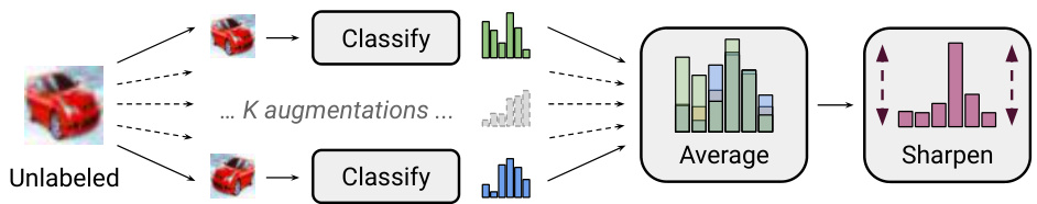
Figure 1: Diagram of the label guessing process used in MixMatch. Stochastic data augmentation is applied to an unlabeled image $K$ times, and each augmented image is fed through the classifier. Then, the average of these $K$ predictions is “sharpened” by adjusting the distribution’s temperature. See algorithm 1 for a full description.
图 1: MixMatch中使用的标签猜测过程示意图。对未标记图像应用随机数据增强 $K$ 次,每次增强后的图像通过分类器处理。然后,通过调整分布温度对这些 $K$ 次预测的平均值进行"锐化"。完整描述参见算法1。
• Experimentally, we show that MixMatch obtains state-of-the-art results on all standard image benchmarks (section 4.2), and reducing the error rate on CIFAR-10 by a factor of 4; • We further show in an ablation study that MixMatch is greater than the sum of its parts; • We demonstrate in section 4.3 that MixMatch is useful for differential ly private learning, enabling students in the PATE framework [36] to obtain new state-of-the-art results that simultaneously strengthen both privacy guarantees and accuracy.
• 实验表明,MixMatch 在所有标准图像基准测试( section 4.2)中都取得了最先进的结果,并将 CIFAR-10 的错误率降低了 4 倍;
• 我们在消融研究中进一步表明,MixMatch 的效果优于其各部分的总和;
• 我们在 section 4.3 中证明,MixMatch 对差分隐私学习非常有用,使 PATE 框架 [36] 中的学生能够同时增强隐私保证和准确性,从而获得新的最先进结果。
In short, MixMatch introduces a unified loss term for unlabeled data that seamlessly reduces entropy while maintaining consistency and remaining compatible with traditional regular iz ation techniques.
简而言之,MixMatch为无标签数据引入了一个统一的损失项,该损失项在保持一致性并与传统正则化技术兼容的同时,还能无缝降低熵值。
2 Related Work
2 相关工作
To set the stage for MixMatch, we first introduce existing methods for SSL. We focus mainly on those which are currently state-of-the-art and that MixMatch builds on; there is a wide literature on SSL techniques that we do not discuss here (e.g., “trans duct ive” models [14, 22, 21], graph-based methods [49, 4, 29], generative modeling [3, 27, 41, 9, 17, 23, 38, 34, 42], etc.). More comprehensive overviews are provided in [49, 6]. In the following, we will refer to a generic model $\mathrm{p}_{\mathrm{model}}(y\mid x;\theta)$ which produces a distribution over class labels $y$ for an input $x$ with parameters $\theta$ .
为介绍MixMatch方法,我们首先回顾现有的半监督学习(SSL)技术。本文主要关注当前最先进且MixMatch所基于的方法,其他SSL技术(如转导模型[14, 22, 21]、基于图的方法[49, 4, 29]、生成式建模[3, 27, 41, 9, 17, 23, 38, 34, 42]等)不在讨论范围内。更全面的综述可参考[49, 6]。下文将使用通用模型$\mathrm{p}_{\mathrm{model}}(y\mid x;\theta)$表示参数为$\theta$的模型对输入$x$输出类别标签$y$的概率分布。
2.1 Consistency Regular iz ation
2.1 一致性正则化 (Consistency Regularization)
A common regular iz ation technique in supervised learning is data augmentation, which applies input transformations assumed to leave class semantics unaffected. For example, in image classification, it is common to elastically deform or add noise to an input image, which can dramatically change the pixel content of an image without altering its label [7, 43, 10]. Roughly speaking, this can artificially expand the size of a training set by generating a near-infinite stream of new, modified data. Consistency regular iz ation applies data augmentation to semi-supervised learning by leveraging the idea that a classifier should output the same class distribution for an unlabeled example even after it has been augmented. More formally, consistency regular iz ation enforces that an unlabeled example $x$ should be classified the same as ${\mathrm{Augment}}(x)$ , an augmentation of itself.
监督学习中一种常见的正则化技术是数据增强(data augmentation),该方法通过应用输入变换来保持类别语义不受影响。例如在图像分类任务中,通常会采用弹性变形或添加噪声等方式处理输入图像,这些操作能在不改变图像标签的前提下显著改变其像素内容[7,43,10]。从本质上说,这种方法能通过生成近乎无限的新增修改数据,人为地扩大训练集规模。一致性正则化(consistency regularization)将数据增强应用于半监督学习,其核心思想是分类器应对未标注样本及其增强版本输出相同的类别分布。更形式化地说,一致性正则化要求未标注样本$x$应与自身增强版本${\mathrm{Augment}}(x)$获得相同的分类结果。
In the simplest case, for unlabeled points $x$ , prior work [25, 40] adds the loss term
对于未标注点$x$的最简单情况,先前工作[25, 40]添加了损失项
$$
|{\mathrm{p}}{\mathrm{model}}(y\mid{\mathrm{Augment}}(x);\theta)-{\mathrm{p}}{\mathrm{model}}(y\mid{\mathrm{Augment}}(x);\theta)|_{2}^{2}.
$$
$$
|{\mathrm{p}}{\mathrm{model}}(y\mid{\mathrm{Augment}}(x);\theta)-{\mathrm{p}}{\mathrm{model}}(y\mid{\mathrm{Augment}}(x);\theta)|_{2}^{2}.
$$
Note that ${\mathrm{Augment}}(x)$ is a stochastic transformation, so the two terms in eq. (1) are not identical. “Mean Teacher” [44] replaces one of the terms in eq. (1) with the output of the model using an exponential moving average of model parameter values. This provides a more stable target and was found empirically to significantly improve results. A drawback to these approaches is that they use domain-specific data augmentation strategies. “Virtual Adversarial Training” [31] (VAT) addresses this by instead computing an additive perturbation to apply to the input which maximally changes the output class distribution. MixMatch utilizes a form of consistency regular iz ation through the use of standard data augmentation for images (random horizontal flips and crops).
请注意 ${\mathrm{Augment}}(x)$ 是一种随机变换,因此等式 (1) 中的两项并不相同。"Mean Teacher" [44] 将等式 (1) 中的一项替换为使用模型参数指数移动平均值的模型输出。这提供了更稳定的目标,并根据经验发现能显著改善结果。这些方法的缺点在于它们使用了特定领域的数据增强策略。"Virtual Adversarial Training" [31] (VAT) 通过计算一个使输出类别分布变化最大的加性扰动来解决这个问题。MixMatch 通过对图像使用标准数据增强 (随机水平翻转和裁剪) 来实现一种形式的正则化一致性。
2.2 Entropy Minimization
2.2 熵最小化
A common underlying assumption in many semi-supervised learning methods is that the classifier’s decision boundary should not pass through high-density regions of the marginal data distribution.
许多半监督学习方法的共同潜在假设是,分类器的决策边界不应穿过边缘数据分布的高密度区域。
One way to enforce this is to require that the classifier output low-entropy predictions on unlabeled data. This is done explicitly in [18] with a loss term which minimizes the entropy of $\operatorname{p}_{\mathrm{model}}(y\mid x;\theta)$ for unlabeled data $x$ . This form of entropy minimization was combined with VAT in [31] to obtain stronger results. “Pseudo-Label” [28] does entropy minimization implicitly by constructing hard (1-hot) labels from high-confidence predictions on unlabeled data and using these as training targets in a standard cross-entropy loss. MixMatch also implicitly achieves entropy minimization through the use of a “sharpening” function on the target distribution for unlabeled data, described in section 3.2.
一种强制执行方法是要求分类器对未标记数据输出低熵预测。[18]中明确采用了一种损失项来实现这一点,该损失项最小化未标记数据$x$的$\operatorname{p}_{\mathrm{model}}(y\mid x;\theta)$熵。这种形式的熵最小化与[31]中的虚拟对抗训练(VAT)结合,获得了更强的结果。"Pseudo-Label"[28]通过从高置信度未标记数据预测中构建硬(one-hot)标签,并在标准交叉熵损失中将其用作训练目标,从而隐式实现了熵最小化。MixMatch也通过3.2节描述的未标记数据目标分布"锐化"函数隐式实现了熵最小化。
2.3 Traditional Regular iz ation
2.3 传统正则化
Regular iz ation refers to the general approach of imposing a constraint on a model to make it harder to memorize the training data and therefore hopefully make it generalize better to unseen data [19]. We use weight decay which penalizes the $L_{2}$ norm of the model parameters [30, 46]. We also use MixUp [47] in MixMatch to encourage convex behavior “between” examples. We utilize MixUp as both as a regularize r (applied to labeled datapoints) and a semi-supervised learning method (applied to unlabeled datapoints). MixUp has been previously applied to semi-supervised learning; in particular, the concurrent work of [45] uses a subset of the methodology used in MixMatch. We clarify the differences in our ablation study (section 4.2.3).
正则化 (regularization) 是指通过对模型施加约束使其更难记住训练数据,从而有望提升对未见数据的泛化能力的通用方法 [19]。我们采用权重衰减 (weight decay) 来惩罚模型参数的 $L_{2}$ 范数 [30, 46]。在 MixMatch 中我们还使用 MixUp [47] 来促进样本"之间"的凸行为。我们将 MixUp 同时作为正则化器 (应用于标注数据点) 和半监督学习方法 (应用于未标注数据点) 使用。MixUp 此前已被应用于半监督学习,特别是同期研究 [45] 采用了 MixMatch 方法中的部分技术。我们将在消融研究 (章节 4.2.3) 中阐明这些差异。
3 MixMatch
3 MixMatch
In this section, we introduce MixMatch, our proposed semi-supervised learning method. MixMatch is a “holistic” approach which incorporates ideas and components from the dominant paradigms for SSL discussed in section 2. Given a batch $\mathcal{X}$ of labeled examples with one-hot targets (representing one of $L$ possible labels) and an equally-sized batch $\mathcal{U}$ of unlabeled examples, MixMatch produces a processed batch of augmented labeled examples $\mathcal{X}^{\prime}$ and a batch of augmented unlabeled examples with “guessed” labels $\mathcal{U}^{\prime},\mathcal{U}^{\prime}$ and $\mathcal{X}^{\prime}$ are then used in computing separate labeled and unlabeled loss terms. More formally, the combined loss $\mathcal{L}$ for semi-supervised learning is defined as
在本节中,我们将介绍提出的半监督学习方法MixMatch。MixMatch是一种"整体性"方法,融合了第2节讨论的主流半监督学习(SSL)范式的思想和组件。给定一个带独热目标(表示L个可能标签之一)的标记样本批次$\mathcal{X}$和同等大小的未标记样本批次$\mathcal{U}$,MixMatch会生成增强后的标记样本批次$\mathcal{X}^{\prime}$和带有"猜测"标签的增强未标记样本批次$\mathcal{U}^{\prime}$。随后$\mathcal{U}^{\prime}$和$\mathcal{X}^{\prime}$将分别用于计算标记和未标记的损失项。更正式地说,半监督学习的组合损失$\mathcal{L}$定义为
$$
\begin{array}{r l}&{\mathcal{X}^{\prime},\mathcal{U}^{\prime}=\displaystyle\mathrm{MixMatch}(\mathcal{X},\mathcal{U},T,K,\alpha)}\ &{\quad\mathcal{L}_{\mathcal{X}}=\displaystyle\frac{1}{|\mathcal{X}^{\prime}|}\sum_{\boldsymbol{x},\boldsymbol{p}\in\mathcal{X}^{\prime}}\mathrm{H}(\boldsymbol{p},\mathrm{p}_{\mathrm{model}}(\boldsymbol{y}\mid\boldsymbol{x};\boldsymbol{\theta}))}\ &{\quad\mathcal{L}_{\mathcal{U}}=\displaystyle\frac{1}{L|\mathcal{U}^{\prime}|}\sum_{\boldsymbol{u},\boldsymbol{q}\in\mathcal{U}^{\prime}}|\boldsymbol{q}-\mathrm{p}_{\mathrm{model}}(\boldsymbol{y}\mid\boldsymbol{u};\boldsymbol{\theta})|_{2}^{2}}\ &{\quad\textit{\textbf{c}},\quad\textit{\textbf{\textit{\textbf{\textit{\textbf{\imath}}}}}},\quad\alpha}\end{array}
$$
$$
\mathcal{L}=\mathcal{L}{\mathcal{X}}+\lambda_{\mathcal{U}}\mathcal{L}_{\mathcal{U}}
$$
$$
\mathcal{L}=\mathcal{L}{\mathcal{X}}+\lambda_{\mathcal{U}}\mathcal{L}_{\mathcal{U}}
$$
where $\mathrm{H}(p,q)$ is the cross-entropy between distributions $p$ and $q$ , and $T,K,\alpha$ , and $\lambda_{\mathcal{U}}$ are hyperparameters described below. The full MixMatch algorithm is provided in algorithm 1, and a diagram of the label guessing process is shown in fig. 1. Next, we describe each part of MixMatch.
其中 $\mathrm{H}(p,q)$ 表示分布 $p$ 和 $q$ 之间的交叉熵,$T,K,\alpha$ 以及 $\lambda_{\mathcal{U}}$ 是下文将描述的超参数。完整的 MixMatch 算法如算法 1 所示,标签猜测过程的示意图见图 1。接下来我们将介绍 MixMatch 的各个部分。
3.1 Data Augmentation
3.1 数据增强
As is typical in many SSL methods, we use data augmentation both on labeled and unlabeled data. For each $x_{b}$ in the batch of labeled data $\mathcal{X}$ , we generate a transformed version $\hat{x}{b}=\mathrm{Augment}(x_{b})$ (algorithm 1, line 3). For each $u_{b}$ in the batch of unlabeled data $\mathcal{U}$ , we generate $K$ augmentations ${{\hat{u}}{b,k}}=\mathrm{Augment}({u_{b}}),k\in(1,\ldots,K)$ (algorithm 1, line 5). We use these individual augmentations to generate a “guessed label” $q_{b}$ for each $u_{b}$ , through a process we describe in the following subsection.
与许多SSL方法类似,我们对标注数据和未标注数据都进行了数据增强。对于标注数据批次$\mathcal{X}$中的每个$x_{b}$,生成变换版本$\hat{x}{b}=\mathrm{Augment}(x_{b})$(算法1第3行)。对于未标注数据批次$\mathcal{U}$中的每个$u_{b}$,生成$K$个增强版本${{\hat{u}}{b,k}}=\mathrm{Augment}({u_{b}}),k\in(1,\ldots,K)$(算法1第5行)。我们通过这些独立增强样本为每个$u_{b}$生成"猜测标签"$q_{b}$,具体过程将在下个小节说明。
3.2 Label Guessing
3.2 标签猜测
For each unlabeled example in $\mathcal{U}$ , MixMatch produces a “guess” for the example’s label using the model’s predictions. This guess is later used in the unsupervised loss term. To do so, we compute the average of the model’s predicted class distributions across all the $K$ augmentations of $u_{b}$ by
对于 $\mathcal{U}$ 中的每个未标注样本,MixMatch 利用模型预测为该样本生成一个"猜测"标签。这一猜测后续将用于无监督损失项。具体实现时,我们通过计算模型对 $u_{b}$ 所有 $K$ 次增强版本的预测类别分布平均值来实现。
$$
\bar{q}{b}=\frac{1}{K}\sum_{k=1}^{K}\operatorname{p}{\operatorname{model}}(y\mid\hat{u}_{b,k};\theta)
$$
$$
\bar{q}{b}=\frac{1}{K}\sum_{k=1}^{K}\operatorname{p}{\operatorname{model}}(y\mid\hat{u}_{b,k};\theta)
$$
in algorithm 1, line 7. Using data augmentation to obtain an artificial target for an unlabeled example is common in consistency regular iz ation methods [25, 40, 44].
在算法1第7行中,使用数据增强为未标注样本生成人工目标是一致性正则化方法中的常见做法 [25, 40, 44]。
Algorithm 1 MixMatch takes a batch of labeled data $\mathcal{X}$ and a batch of unlabeled data $\mathcal{U}$ and produces a collection $\mathcal{X}^{\prime}$ (resp. $\mathcal{U}^{\prime}$ ) of processed labeled examples (resp. unlabeled with guessed labels).
算法 1 MixMatch 接收一批带标签数据 $\mathcal{X}$ 和一批无标签数据 $\mathcal{U}$ ,生成处理后的带标签样本集合 $\mathcal{X}^{\prime}$ (对应地,无标签样本的猜测标签集合 $\mathcal{U}^{\prime}$ )。
Sharpening. In generating a label guess, we perform one additional step inspired by the success of entropy minimization in semi-supervised learning (discussed in section 2.2). Given the average prediction over augmentations $\bar{q}_{b}$ , we apply a sharpening function to reduce the entropy of the label distribution. In practice, for the sharpening function, we use the common approach of adjusting the “temperature” of this categorical distribution [16], which is defined as the operation
锐化。在生成标签猜测时,我们额外增加了一个步骤,其灵感来自于半监督学习中熵最小化的成功(在第2.2节中讨论)。给定数据增强的平均预测 $\bar{q}_{b}$ ,我们应用锐化函数来降低标签分布的熵。实际上,对于锐化函数,我们采用了调整分类分布"温度"的常见方法 [16],其定义为操作
$$
{\mathrm{Sharpen}}(p,T){i}:=p_{i}^{\frac{1}{T}}{\Bigg/}\sum_{j=1}^{L}p_{j}^{\frac{1}{T}}
$$
$$
{\mathrm{Sharpen}}(p,T){i}:=p_{i}^{\frac{1}{T}}{\Bigg/}\sum_{j=1}^{L}p_{j}^{\frac{1}{T}}
$$
where $p$ is some input categorical distribution (specifically in MixMatch, $p$ is the average class prediction over augmentations $\bar{q}{b}$ , as shown in algorithm 1, line 8) and $T$ is a hyper parameter. As $T\rightarrow0$ , the output of ${\mathrm{Sharpen}}(p,T)$ will approach a Dirac (“one-hot”) distribution. Since we will later use $q_{b}=\mathrm{Sharpen}(\bar{q}{b},T)$ as a target for the model’s prediction for an augmentation of $u_{b}$ , lowering the temperature encourages the model to produce lower-entropy predictions.
其中 $p$ 是某个输入分类分布 (在 MixMatch 中特指增强预测的平均类别概率 $\bar{q}{b}$,如算法 1 第 8 行所示),$T$ 是超参数。当 $T\rightarrow0$ 时,${\mathrm{Sharpen}}(p,T)$ 的输出将趋近狄拉克 ("独热") 分布。由于后续我们将使用 $q_{b}=\mathrm{Sharpen}(\bar{q}{b},T)$ 作为模型对 $u_{b}$ 增强样本的预测目标,降低温度参数会促使模型产生更低熵的预测结果。
3.3 MixUp
3.3 MixUp
We use MixUp for semi-supervised learning, and unlike past work for SSL we mix both labeled examples and unlabeled examples with label guesses (generated as described in section 3.2). To be compatible with our separate loss terms, we define a slightly modified version of MixUp. For a pair of two examples with their corresponding labels probabilities $(x_{1},p_{1}),(x_{2},p_{2})$ we compute $(x^{\prime},p^{\prime})$ by
我们在半监督学习中使用MixUp方法,与以往SSL (Semi-Supervised Learning) 工作不同,我们会混合带标签样本和带有标签猜测(生成方式如第3.2节所述)的无标签样本。为了兼容我们独立的损失项,我们定义了一个略微修改版的MixUp。对于一对样本及其对应的标签概率 $(x_{1},p_{1}),(x_{2},p_{2})$,我们通过计算得到 $(x^{\prime},p^{\prime})$
$$
\begin{array}{l}{{\lambda\sim\mathrm{Beta}(\alpha,\alpha)}}\ {{\lambda^{\prime}=\operatorname*{max}(\lambda,1-\lambda)}}\ {{x^{\prime}=\lambda^{\prime}x_{1}+(1-\lambda^{\prime})x_{2}}}\ {{p^{\prime}=\lambda^{\prime}p_{1}+(1-\lambda^{\prime})p_{2}}}\end{array}
$$
$$
\begin{array}{l}{{\lambda\sim\mathrm{Beta}(\alpha,\alpha)}}\ {{\lambda^{\prime}=\operatorname*{max}(\lambda,1-\lambda)}}\ {{x^{\prime}=\lambda^{\prime}x_{1}+(1-\lambda^{\prime})x_{2}}}\ {{p^{\prime}=\lambda^{\prime}p_{1}+(1-\lambda^{\prime})p_{2}}}\end{array}
$$
where $\alpha$ is a hyper parameter. Vanilla MixUp omits eq. (9) (i.e. it sets $\lambda^{\prime}=\lambda$ ). Given that labeled and unlabeled examples are concatenated in the same batch, we need to preserve the order of the batch to compute individual loss components appropriately. This is achieved by eq. (9) which ensures that $x^{\prime}$ is closer to $x_{1}$ than to $x_{2}$ . To apply MixUp, we first collect all augmented labeled examples with their labels and all unlabeled examples with their guessed labels into
其中$\alpha$是一个超参数。原始MixUp忽略了公式(9)(即设$\lambda^{\prime}=\lambda$)。由于标注样本和无标注样本在同一个批次中被拼接,我们需要保持批次顺序以正确计算各损失分量。公式(9)通过确保$x^{\prime}$更接近$x_{1}$而非$x_{2}$来实现这一点。应用MixUp时,我们首先将所有增强的标注样本及其标签、所有无标注样本及其猜测标签收集到
$$
\begin{array}{r l}&{\hat{\mathcal{X}}=\left((\hat{x}{b},p_{b});b\in(1,\ldots,B)\right)}\ &{\hat{\mathcal{U}}=\left((\hat{u}{b,k},q_{b});b\in(1,\ldots,B),k\in(1,\ldots,K)\right)}\end{array}
$$
$$
\begin{array}{r l}&{\hat{\mathcal{X}}=\left((\hat{x}{b},p_{b});b\in(1,\ldots,B)\right)}\ &{\hat{\mathcal{U}}=\left((\hat{u}{b,k},q_{b});b\in(1,\ldots,B),k\in(1,\ldots,K)\right)}\end{array}
$$
(algorithm 1, lines 10–11). Then, we combine these collections and shuffle the result to form $\mathcal{W}$ which will serve as a data source for MixUp (algorithm 1, line 12). For each the $i^{t h}$ example-label pair in $\hat{\mathcal X}$ , we compute $\mathrm{MixUp}(\hat{\mathcal{X}}{i},\mathcal{W}{i})$ and add the result to the collection $\mathcal{X}^{\prime}$ (algorithm 1, line 13). We compute $\mathcal{U}{i}^{\prime}=\mathrm{MixUp}(\hat{\mathcal{U}}{i},\mathcal{W}_{i+|\hat{\mathcal{X}}|})$ for $i\in(1,\dots,|\hat{\mathcal{U}}|)$ , intentionally using the remainder of $\mathcal{W}$ that was not used in the construction of $\mathcal{X}^{\prime}$ (algorithm 1, line 14). To summarize, MixMatch transforms $\mathcal{X}$ into $\mathcal{X}^{\prime}$ , a collection of labeled examples which have had data augmentation and MixUp (potentially mixed with an unlabeled example) applied. Similarly, $\mathcal{U}$ is transformed into $\mathcal{U}^{\prime}$ , a collection of multiple augmentations of each unlabeled example with corresponding label guesses.
(算法1,第10-11行)。接着,我们将这些集合合并并打乱顺序,形成作为MixUp数据源的$\mathcal{W}$(算法1,第12行)。对于$\hat{\mathcal X}$中的每个第$i^{t h}$个样本-标签对,我们计算$\mathrm{MixUp}(\hat{\mathcal{X}}{i},\mathcal{W}{i})$并将结果加入集合$\mathcal{X}^{\prime}$(算法1,第13行)。同时,针对$i\in(1,\dots,|\hat{\mathcal{U}}|)$,我们计算$\mathcal{U}{i}^{\prime}=\mathrm{MixUp}(\hat{\mathcal{U}}{i},\mathcal{W}_{i+|\hat{\mathcal{X}}|})$,这里特意使用$\mathcal{W}$中未被用于构建$\mathcal{X}^{\prime}$的剩余部分(算法1,第14行)。总结来说,MixMatch将$\mathcal{X}$转换为$\mathcal{X}^{\prime}$——一个经过数据增强和MixUp(可能与无标签样本混合)处理的带标签样本集合;类似地,$\mathcal{U}$被转换为$\mathcal{U}^{\prime}$——每个无标签样本经多次增强并带有对应预测标签的集合。
3.4 Loss Function
3.4 损失函数
Given our processed batches $\mathcal{X}^{\prime}$ and $\mathcal{U}^{\prime}$ , we use the standard semi-supervised loss shown in eqs. (3) to (5). Equation (5) combines the typical cross-entropy loss between labels and model predictions from $\mathcal{X}^{\prime}$ with the squared $L_{2}$ loss on predictions and guessed labels from $\mathcal{U}^{\prime}$ . We use this $L_{2}$ loss in eq. (4) (the multiclass Brier score [5]) because, unlike the cross-entropy, it is bounded and less sensitive to incorrect predictions. For this reason, it is often used as the unlabeled data loss in SSL [25, 44] as well as a measure of predictive uncertainty [26]. We do not propagate gradients through computing the guessed labels, as is standard [25, 44, 31, 35]
给定处理后的批次 $\mathcal{X}^{\prime}$ 和 $\mathcal{U}^{\prime}$,我们使用公式 (3) 至 (5) 所示的标准半监督损失函数。公式 (5) 将 $\mathcal{X}^{\prime}$ 中标签与模型预测的常规交叉熵损失,与 $\mathcal{U}^{\prime}$ 中预测值和猜测标签的平方 $L_{2}$ 损失相结合。我们在公式 (4) 中使用这种 $L_{2}$ 损失(多分类 Brier 分数 [5]),因为与交叉熵不同,它是有界的且对错误预测的敏感性较低。因此,它常被用作半监督学习 (SSL) 中的无标签数据损失 [25, 44],以及预测不确定性的度量 [26]。按照惯例 [25, 44, 31, 35],我们不会通过计算猜测标签来传播梯度。
3.5 Hyper parameters
3.5 超参数
Since MixMatch combines multiple mechanisms for leveraging unlabeled data, it introduces various hyper parameters – specifically, the sharpening temperature $T$ , number of unlabeled augmentations $K$ , $\alpha$ parameter for Beta in MixUp, and the unsupervised loss weight $\lambda_{\mathcal{U}}$ . In practice, semi-supervised learning methods with many hyper parameters can be problematic because cross-validation is difficult with small validation sets [35, 39, 35]. However, we find in practice that most of MixMatch’s hyper parameters can be fixed and do not need to be tuned on a per-experiment or per-dataset basis. Specifically, for all experiments we set $T=0.5$ and $K=2$ . Further, we only change $\alpha$ and $\lambda_{\mathcal{U}}$ on a per-dataset basis; we found that $\alpha=0.75$ and $\lambda_{\mathcal{U}}=100$ are good starting points for tuning. In all experiments, we linearly ramp up $\lambda_{\mathcal{U}}$ to its maximum value over the first 16,000 steps of training as is common practice [44].
由于MixMatch结合了多种利用未标记数据的机制,它引入了多个超参数——具体包括锐化温度 $T$ 、未标记数据增强次数 $K$ 、MixUp中Beta分布的 $\alpha$ 参数,以及无监督损失权重 $\lambda_{\mathcal{U}}$ 。实践中,具有大量超参数的半监督学习方法可能存在问题,因为在小规模验证集上难以进行交叉验证[35, 39, 35]。但我们发现MixMatch的大部分超参数可固定使用,无需针对每个实验或数据集单独调整。具体而言,所有实验中我们设定 $T=0.5$ 和 $K=2$ 。此外,仅根据数据集调整 $\alpha$ 和 $\lambda_{\mathcal{U}}$ ——我们发现 $\alpha=0.75$ 和 $\lambda_{\mathcal{U}}=100$ 是良好的调优起点。按照常规做法[44],所有实验均在训练前16,000步线性提升 $\lambda_{\mathcal{U}}$ 至最大值。
4 Experiments
4 实验
We test the effectiveness of MixMatch on standard SSL benchmarks (section 4.2). Our ablation study teases apart the contribution of each of MixMatch’s components (section 4.2.3). As an additional application, we consider privacy-preserving learning in section 4.3.
我们在标准半监督学习基准测试中验证了MixMatch的有效性(见4.2节)。消融实验解析了MixMatch各组件的作用(见4.2.3节)。作为延伸应用,我们在4.3节探讨了隐私保护学习场景。
4.1 Implementation details
4.1 实现细节
Unless otherwise noted, in all experiments we use the “Wide ResNet-28” model from [35]. Our implementation of the model and training procedure closely matches that of [35] (including using 5000 examples to select the hyper parameters), except for the following differences: First, instead of decaying the learning rate, we evaluate models using an exponential moving average of their parameters with a decay rate of 0.999. Second, we apply a weight decay of 0.0004 at each update for the Wide ResNet-28 model. Finally, we checkpoint every $2^{16}$ training samples and report the median error rate of the last 20 checkpoints. This simplifies the analysis at a potential cost to accuracy by, for example, averaging checkpoints [2] or choosing the checkpoint with the lowest validation error.
除非另有说明,所有实验中我们均使用[35]提出的"Wide ResNet-28"模型。我们的模型实现与训练流程基本遵循[35]的方案(包括使用5000个样本选择超参数),仅存在以下差异:首先,我们不再衰减学习率,而是采用衰减率为0.999的参数指数移动平均值来评估模型;其次,Wide ResNet-28模型每次更新时应用0.0004的权重衰减;最后,每训练$2^{16}$个样本保存一次检查点,并报告最后20个检查点的错误率中位数。这种做法简化了分析流程,但可能牺牲部分准确性,例如未采用检查点平均[2]或选择验证误差最低的检查点等优化手段。
4.2 Semi-Supervised Learning
4.2 半监督学习
First, we evaluate the effectiveness of MixMatch on four standard benchmark datasets: CIFAR-10 and CIFAR-100 [24], SVHN [32], and STL-10 [8]. Standard practice for evaluating semi-supervised learning on the first three datasets is to treat most of the dataset as unlabeled and use a small portion as labeled data. STL-10 is a dataset specifically designed for SSL, with 5,000 labeled images and 100,000 unlabeled images which are drawn from a slightly different distribution than the labeled data.
首先,我们在四个标准基准数据集上评估MixMatch的效果:CIFAR-10和CIFAR-100 [24]、SVHN [32]以及STL-10 [8]。前三个数据集评估半监督学习的标准做法是将大部分数据视为未标记,仅使用一小部分作为标记数据。STL-10是专为SSL设计的数据集,包含5,000张标记图像和100,000张未标记图像,这些未标记图像与标记数据的分布略有不同。
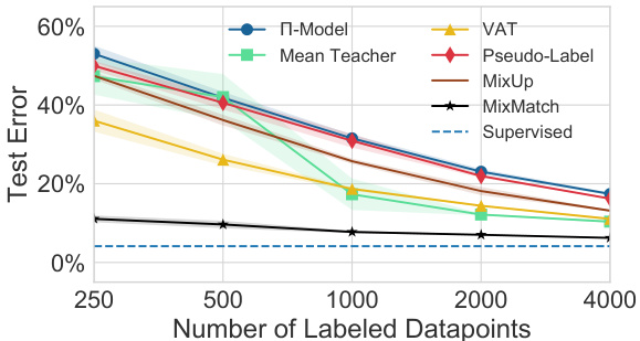
Figure 2: Error rate comparison of MixMatch to baseline methods on CIFAR-10 for a varying number of labels. Exact numbers are provided in table 5 (appendix). “Supervised” refers to training with all 50000 training examples and no unlabeled data. With 250 labels MixMatch reaches an error rate comparable to next-best method’s performance with 4000 labels.
图 2: CIFAR-10数据集上MixMatch与基线方法在不同标签数量下的错误率对比。具体数值见表5(附录)。"Supervised"表示使用全部50000个训练样本且不使用未标注数据进行训练。当仅使用250个标签时,MixMatch达到的错误率与次优方法使用4000个标签时的性能相当。
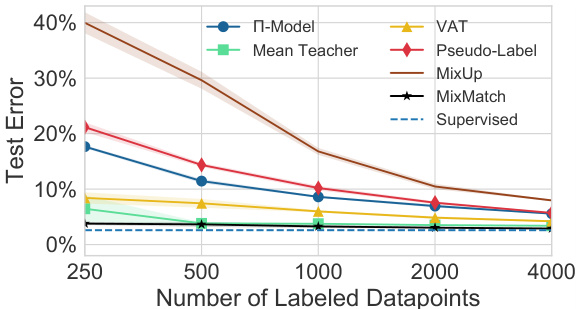
Figure 3: Error rate comparison of MixMatch to baseline methods on SVHN for a varying number of labels. Exact numbers are provided in table 6 (appendix). “Supervised” refers to train-ing with all 73257 training examples and no unlabeled data. With 250 examples MixMatch nearly reaches the accuracy of supervised training for this model.
图 3: MixMatch与基线方法在SVHN数据集上随标签数量变化的错误率对比。具体数值见表6(附录)。"Supervised"表示使用全部73257个训练样本且无未标注数据的训练结果。当使用250个样本时,MixMatch几乎达到了该模型在监督训练下的准确率。
4.2.1 Baseline Methods
4.2.1 基线方法
As baselines, we consider the four methods considered in [35] (Π-Model [25, 40], Mean Teacher [44], Virtual Adversarial Training [31], and Pseudo-Label [28]) which are described in section 2. We also use MixUp [47] on its own as a baseline. MixUp is designed as a regularize r for supervised learning, so we modify it for SSL by applying it both to augmented labeled examples and augmented unlabeled examples with their corresponding predictions. In accordance with standard usage of MixUp, we use a cross-entropy loss between the MixUp-generated guess label and the model’s prediction. As advocated by [35], we re implemented each of these methods in the same codebase and applied them to the same model (described in section 4.1) to ensure a fair comparison. We re-tuned the hyper parameters for each baseline method, which generally resulted in a marginal accuracy improvement compared to those in [35], thereby providing a more competitive experimental setting for testing out MixMatch.
作为基线方法,我们采用[35]中涉及的四种方法(Π-Model [25, 40]、Mean Teacher [44]、Virtual Adversarial Training [31]和Pseudo-Label [28]),这些方法在第2节已有描述。同时,我们将MixUp [47]单独作为基线使用。MixUp原本是监督学习中的正则化方法,我们通过将其同时应用于增强后的标注样本和带有预测结果的未标注样本,使其适用于半监督学习(SSL)。按照MixUp的标准用法,我们在混合生成的猜测标签与模型预测之间采用交叉熵损失。如[35]所建议,我们在同一代码库中重新实现了每种方法,并将其应用于同一模型(见第4.1节描述)以确保公平比较。我们为每个基线方法重新调整了超参数,相比[35]的结果普遍获得了小幅精度提升,从而为测试MixMatch提供了更具竞争力的实验环境。
4.2.2 Results
4.2.2 结果
CIFAR-10 For CIFAR-10, we evaluate the accuracy of each method with a varying number of labeled examples from 250 to 4000 (as is standard practice). The results can be seen in fig. 2. We used $\lambda_{\mathcal{U}}=75$ for CIFAR-10. We created 5 splits for each number of labeled points, each with a different random seed. Each model was trained on each split and the error rates were reported by the mean and variance across splits. We find that MixMatch outperforms all other methods by a significant margin, for example reaching an error rate of $6.24%$ with 4000 labels. For reference, on the same model, fully supervised training on all 50000 samples achieves an error rate of $4.17%$ Furthermore, MixMatch obtains an error rate of $11.08%$ with only 250 labels. For comparison, at 250 labels the next-best-performing method (VAT [31]) achieves an error rate of 36.03, over $4.5\times$ higher than MixMatch considering that $4.17%$ is the error limit obtained on our model with fully supervised learning. In addition, at 4000 labels the next-best-performing method (Mean Teacher [44]) obtains an error rate of $10.36%$ , which suggests that MixMatch can achieve similar performance with only $1/16$ as many labels. We believe that the most interesting comparisons are with very few labeled data points since it reveals the method’s sample efficiency which is central to SSL.
CIFAR-10
针对CIFAR-10数据集,我们评估了各方法在标注样本量从250到4000(标准实践范围)变化时的准确率,结果如图2所示。实验中设定$\lambda_{\mathcal{U}}=75$,并为每个标注量创建5组不同随机种子的数据划分。每个模型在各划分上训练后,报告误差率的均值和方差。
MixMatch显著优于其他方法:例如在4000标注量时达到$6.24%$的误差率(参考值:同模型在全量50000样本监督训练下误差率为$4.17%$)。仅用250标注量时,MixMatch误差率为$11.08%$,而次优方法(VAT [31])的36.03误差率是其4.5倍以上(以全监督学习的$4.17%$误差极限为基准)。
在4000标注量时,次优方法(Mean Teacher [44])误差率为$10.36%$,表明MixMatch仅需$1/16$标注量即可达到相近性能。我们认为极低标注量下的对比最具意义,因其揭示了半监督学习(SSL)核心的样本效率特性。
CIFAR-10 and CIFAR-100 with a larger model Some prior work [44, 2] has also considered the use of a larger, 26 million-parameter model. Our base model, as used in [35], has only 1.5 million parameters which confounds comparison with these results. For a more reasonable comparison to these results, we measure the effect of increasing the width of our base ResNet model and evaluate MixMatch’s performance on a 28-layer Wide Resnet model which has 135 filters per layer, resulting in 26 million parameters. We also evaluate MixMatch on this larger model on CIFAR-100 with 10000 labels, to compare to the corresponding result from [2]. The results are shown in table 1. In general, MixMatch matches or outperforms the best results from [2], though we note that the comparison still remains problematic due to the fact that the model from [44, 2] also uses more
使用更大模型在CIFAR-10和CIFAR-100上的表现
已有研究[44,2]采用了参数规模达2600万的更大模型。而我们在[35]中使用的基础模型仅含150万参数,这导致与这些结果的直接对比存在困难。为进行更合理的比较,我们通过增加基础ResNet模型宽度进行测试,并在每层含135个滤波器(总计2600万参数)的28层Wide Resnet模型上评估MixMatch性能。同时,我们在含10000个标签的CIFAR-100数据集上使用该大模型评估MixMatch,以对比[2]的对应结果。数据如 表1 所示。总体而言,MixMatch达到或超越了[2]的最佳结果,但需注意由于[44,2]采用的模型还使用了更多...
Table 1: CIFAR-10 and CIFAR-100 error rate (with 4,000 and 10,000 labels respectively) with larger models (26 million parameters).
表 1: 更大模型(2600万参数)在CIFAR-10和CIFAR-100上的错误率(分别使用4000和10000个标签)。
| 方法 | CIFAR-10 | CIFAR-100 |
|---|---|---|
| Mean Teacher [44] SWA [2] | 6.28 5.00 | 28.80 |
| MixMatch | 4.95 ± 0.08 | 25.88 ± 0.30 |
Table 2: STL-10 error rate using 1000-label splits or the entire 5000-label training set.
表 2: 使用1000标签分割或完整5000标签训练集的STL-10错误率
| Method | 1000labels | 5000labels |
|---|---|---|
| CutOut [12] | 12.74 | |
| IIC [20] | 11.20 | |
| SWWAE[48] | 25.70 | |
| CC-GAN2 [11] | 22.20 | 1 |
| MixMatch | 10.18±1.46 | 5.59 |
Table 3: Comparison of error rates for SVHN and $\mathrm{SVHN+}$ Extra for MixMatch. The last column (“All”) contains the fully-supervised performance with all labels in the corresponding training set.
表 3: MixMatch 在 SVHN 和 $\mathrm{SVHN+}$ Extra 数据集上的错误率对比。最后一列 ("All") 表示使用对应训练集中所有标签时的全监督性能。
| Labels | 250 | 500 | 1000 | 2000 | 4000 | All |
|---|---|---|---|---|---|---|
| SVHN | 3.78 ± 0.26 | 3.64 ± 0.46 | 3.27 ± 0.31 | 3.04 ± 0.13 | 2.89 ± 0.06 | 2.59 |
| SVHN+Extra | 2.22 ± 0.08 | 2.17 ± 0.07 | 2.18 ± 0.06 | 2.12 ± 0.03 | 2.07 ± 0.05 | 1.71 |
SVHN and SVHN+Extra As with CIFAR-10, we evaluate the performance of each SSL method on SVHN with a varying number of labels from 250 to 4000. As is standard practice, we first consider the setting where the 73257-example training set is split into labeled and unlabeled data. The results are shown in fig. 3. We used $\lambda_{\mathcal{U}}=250$ . Here again the models were evaluated on 5 splits for each number of labeled points, each with a different random seed. We found MixMatch’s performance to be relatively constant (and better than all other methods) across all amounts of labeled data. Surprisingly, after additional tuning we were able to obtain extremely good performance from Mean Teacher [44], though its error rate was consistently slightly higher than MixMatch’s.
SVHN和SVHN+Extra
与CIFAR-10类似,我们评估了每种SSL方法在SVHN上使用250至4000个不同数量标签的性能。按照标准做法,我们首先考虑将73257个样本的训练集划分为有标签和无标签数据的设置。结果如图3所示。我们使用$\lambda_{\mathcal{U}}=250$。同样,每个标签数量的模型在5个不同的随机种子划分下进行评估。我们发现MixMatch在所有标签数据量下的性能相对稳定(且优于其他所有方法)。出乎意料的是,经过额外调优后,我们能够从Mean Teacher [44]中获得极佳的性能,尽管其错误率始终略高于MixMatch。
Note that SVHN has two training sets: train and extra. In fully-supervised learning, both sets are concatenated to form the full training set (604388 samples). In SSL, for historical reasons the extra set was left aside and only train was used (73257 samples). We argue that leveraging both train and extra for the unlabeled data is more interesting since it exhibits a higher ratio of unlabeled samples over labeled ones. We report error rates for both SVHN and SVHN $+$ Extra in table 3. For SVHN $^+$ Extra we used $\alpha=0.25$ , $\lambda_{\mathcal{U}}=250$ and a lower weight decay of 0.000002 due to the larger amount of available data. We found that on both training sets, MixMatch nearly matches the fully-supervised performance on the same training set almost immediately – for example, MixMatch achieves an error rate of $2.22%$ with only 250 labels on SVHN+Extra compared to the fully-supervised performance of $1.71%$ . Interestingly, on SVHN+Extra MixMatch outperformed fully supervised training on SVHN without extra $(2.59%$ error) for every labeled data amount considered. To emphasize the importance of this, consider the following scenario: You have 73257 examples from SVHN with 250 examples labeled and are given a choice: You can either obtain $8\times$ more unlabeled data and use MixMatch or obtain $293\times$ more labeled data and use fully-supervised learning. Our results suggest that obtaining additional unlabeled data and using MixMatch is more effective, which conveniently is likely much cheaper than obtaining $293\times$ more labels.
请注意,SVHN 包含两个训练集:train 和 extra。在全监督学习中,这两个集合会被合并为完整训练集(共 604388 个样本)。而在半监督学习 (SSL) 中,由于历史原因,extra 集通常被单独保留,仅使用 train 集(73257 个样本)。我们认为同时利用 train 和 extra 作为未标注数据更具研究价值,因为这样可以获得更高的未标注样本与标注样本比例。表 3 展示了 SVHN 和 SVHN $+$ Extra 的错误率结果。对于 SVHN $^+$ Extra,我们设定 $\alpha=0.25$、$\lambda_{\mathcal{U}}=250$,并由于数据量更大而采用较低的权重衰减值 0.000002。研究发现,在两个训练集上,MixMatch 几乎能立即达到与全监督方法在该训练集上相当的性能——例如在 SVHN+Extra 上仅用 250 个标注样本时,MixMatch 的错误率为 $2.22%$,而全监督方法的错误率为 $1.71%$。值得注意的是,在 SVHN+Extra 上,MixMatch 在所有标注数据量下的表现均优于未使用 extra 集的全监督训练结果 $(2.59%$ 错误率)。为强调这一发现的重要性,设想以下场景:您拥有 SVHN 的 73257 个样本,其中 250 个已标注,现在有两种选择:要么获取 $8\times$ 倍未标注数据并使用 MixMatch,要么获取 $293\times$ 倍标注数据并采用全监督学习。我们的结果表明,获取额外未标注数据并使用 MixMatch 更具效益,且其成本显然远低于获取 $293\times$ 倍标注样本。
STL-10 STL-10 contains 5000 training examples aimed at being used with 10 predefined folds (we use the first 5 only) with 1000 examples each. However, some prior work trains on all 5000 examples. We thus compare in both experimental settings. With 1000 examples MixMatch surpasses both the state-of-the-art for 1000 examples as well as the state-of-the-art using all 5000 labeled examples. Note that none of the baselines in table 2 use the same experimental setup (i.e. model), so it is difficult to directly compare the results; however, because MixMatch obtains the lowest error by a factor of two, we take this to be a vote in confidence of our method. We used $\lambda_{\mathcal{U}}=50$ .
STL-10
STL-10包含5000个训练样本,设计用于10个预定义折叠(我们仅使用前5个),每个折叠含1000个样本。但先前部分研究使用了全部5000个样本进行训练。因此我们在两种实验设置下进行比较。使用1000个样本时,MixMatch不仅超越了1000样本量下的最优结果,还超越了使用全部5000个标注样本的最优结果。需注意表2中的基线方法均未采用相同实验设置(即模型),因此难以直接比较结果;但由于MixMatch将错误率降低至原先的一半,我们认为这证明了方法的可靠性。实验中设定$\lambda_{\mathcal{U}}=50$。
4.2.3 Ablation Study
4.2.3 消融研究
Since MixMatch combines various semi-supervised learning mechanisms, it has a good deal in common with existing methods in the literature. As a result, we study the effect of removing or adding components in order to provide additional insight into what makes MixMatch performant. Specifically, we measure the effect of
由于MixMatch结合了多种半监督学习机制,它与文献中的现有方法有许多共同点。因此,我们研究了移除或添加组件的影响,以进一步了解MixMatch的性能来源。具体而言,我们测量了以下因素的影响:
Table 4: Ablation study results. All values are error rates on CIFAR-10 with 250 or 4000 labels.
| 消融实验 | 250标签 | 4000标签 |
|---|---|---|
| MixMatch | 11.80 | 6.00 |
| 无分布平均的MixMatch (K=1) | 17.09 | 8.06 |
| K=3的MixMatch | 11.55 | 6.23 |
| K=4的MixMatch | 12.45 | 5.88 |
| 无温度锐化的MixMatch (T=1) | 27.83 | 10.59 |
| 带参数EMA的MixMatch | 11.86 | 6.47 |
| 无MixUp的MixMatch | 39.11 | 10.97 |
| 仅对标注数据使用MixUp的MixMatch | 32.16 | 9.22 |
| 仅对未标注数据使用MixUp的MixMatch | 12.35 | 6.83 |
| 对标注和未标注数据分别使用MixUp的MixMatch | 12.26 | 6.50 |
| 插值一致性训练 [45] | 38.60 | 6.81 |
表 4: 消融研究结果。所有数值均为CIFAR-10数据集在250或4000标签量下的错误率。
We carried out the ablation on CIFAR-10 with 250 and 4000 labels; the results are shown in table 4. We find that each component contributes to MixMatch’s performance, with the most dramatic differences in the 250-label setting. Despite Mean Teacher’s effectiveness on SVHN (fig. 3), we found that using a similar EMA of parameter values hurt MixMatch’s performance slightly.
我们在CIFAR-10数据集上分别使用250和4000个标签进行了消融实验,结果如表4所示。研究发现,MixMatch的每个组件都对性能有所贡献,其中250标签设置下的差异最为显著。尽管Mean Teacher在SVHN数据集上表现优异(图3),但我们发现采用类似的参数值指数移动平均(EMA)会轻微降低MixMatch的性能。
4.3 Privacy-Preserving Learning and Generalization
4.3 隐私保护学习与泛化
Learning with privacy allows us to measure our approach’s ability to generalize. Indeed, protecting the privacy of training data amounts to proving that the model does not overfit: a learning algorithm is said to be differential ly private (the most widely accepted technical definition of privacy) if adding, modifying, or removing any of its training samples is guaranteed not to result in a statistically significant difference in the model parameters learned [13]. For this reason, learning with differential privacy is, in practice, a form of regular iz ation [33]. Each training data access constitutes a potential privacy leakage, encoded as the pair of the input and its label. Hence, approaches for deep learning from private training data, such as DP-SGD [1] and PATE [36], benefit from accessing as few labeled private training points as possible when computing updates to the model parameters. Semi-supervised learning is a natural fit for this setting.
隐私学习使我们能够衡量方法的泛化能力。事实上,保护训练数据的隐私等同于证明模型不会过拟合:如果保证增加、修改或删除任何训练样本都不会导致学习到的模型参数出现统计学显著差异 [13],则该学习算法被称为差分隐私(最广泛接受的隐私技术定义)。因此,差分隐私学习实际上是一种正则化形式 [33]。每次训练数据访问都构成潜在的隐私泄露,编码为输入及其标签的对。因此,在计算模型参数更新时,访问尽可能少的标记私有训练点对基于私有训练数据的深度学习方法(如 DP-SGD [1] 和 PATE [36])有益。半监督学习天然适合这种场景。
We use the PATE framework for learning with privacy. A student is trained in a semi-supervised way from public unlabeled data, part of which is labeled by an ensemble of teachers with access to private labeled training data. The fewer labels a student requires to reach a fixed accuracy, the stronger is the privacy guarantee it provides. Teachers use a noisy voting mechanism to respond to label queries from the student, and they may choose not to provide a label when they cannot reach a sufficiently strong consensus. For this reason, if MixMatch improves the performance of PATE, it would also illustrate MixMatch’s improved generalization from few canonical exemplars of each class.
我们采用PATE框架进行隐私保护学习。通过半监督方式从公开无标签数据中训练学生模型,其中部分数据由能访问私有带标签训练数据的教师模型集合进行标注。学生模型达到固定准确率所需的标签越少,其提供的隐私保障就越强。教师模型采用带噪声的投票机制响应学生模型的标签查询请求,当无法达成足够强的共识时可以选择不提供标签。因此,若MixMatch能提升PATE的性能,也将证明MixMatch通过各类别的少量典型样本实现了更好的泛化能力。
We compare the accuracy-privacy trade-off achieved by MixMatch to a VAT [31] baseline on SVHN. VAT achieved the previous state-of-the-art of $91.6%$ test accuracy for a privacy loss of $\varepsilon=4.96$ [37]. Because MixMatch performs well with few labeled points, it is able to achieve $95.21\pm0.17%$ test accuracy for a much smaller privacy loss of $\varepsilon=0.97$ . Because $e^{\varepsilon}$ is used to measure the degree of privacy, the improvement is approximately $e^{4}\approx55\times$ , a significant improvement. A privacy loss $\varepsilon$ below 1 corresponds to a much stronger privacy guarantee. Note that in the private training setting the student model only uses 10,000 total examples.
我们在SVHN数据集上比较了MixMatch与VAT [31]基线在准确率-隐私权衡方面的表现。VAT此前以隐私损失$\varepsilon=4.96$ [37]实现了$91.6%$的测试准确率最优水平。由于MixMatch在少量标注数据下表现优异,它能以更低的隐私损失$\varepsilon=0.97$实现$95.21\pm0.17%$的测试准确率。由于使用$e^{\varepsilon}$衡量隐私程度,这一改进约为$e^{4}\approx55\times$,提升显著。隐私损失$\varepsilon$低于1意味着更强的隐私保障。需注意在隐私训练设置中,学生模型仅使用10,000个样本。
5 Conclusion
5 结论
We introduced MixMatch, a semi-supervised learning method which combines ideas and components from the current dominant paradigms for SSL. Through extensive experiments on semi-supervised and privacy-preserving learning, we found that MixMatch exhibited significantly improved performance compared to other methods in all settings we studied, often by a factor of two or more reduction in error rate. In future work, we are interested in incorporating additional ideas from the semi-supervised learning literature into hybrid methods and continuing to explore which components result in effective algorithms. Separately, most modern work on semi-supervised learning algorithms is evaluated on image benchmarks; we are interested in exploring the effectiveness of MixMatch in other domains.
我们提出了MixMatch,这是一种半监督学习方法,融合了当前主流半监督学习(SSL)范式的思路与组件。通过在半监督学习和隐私保护学习场景中的大量实验,我们发现MixMatch在所有研究场景中都显著优于其他方法,错误率通常能降低两倍或更多。未来工作中,我们有意将半监督学习领域的更多思路融入混合方法,并持续探索哪些组件能构成有效算法。另外,当前多数半监督学习算法的研究都基于图像基准测试,我们计划探索MixMatch在其他领域的有效性。
Acknowledgement
致谢
We would like to thank Balaji Lakshmi narayan an for his helpful theoretical insights.
我们要感谢 Balaji Lakshmi narayan an 提供的宝贵理论见解。
References
参考文献
A Notation and definitions
符号与定义
| 符号 | 定义 |
|---|---|
| H(p, q) | |
| C | 带标签的样本,作为模型输入 |
| p | (独热)标签 |
| L | 可能的标签类别数量(p的维度) |
| 一批带标签样本及其标签 | |
| 七 | MixMatch生成的已处理带标签样本批次 |
| u | 无标签样本,作为模型输入 |
| q | 无标签样本的猜测标签分布 |
| u | 无标签样本批次 |
| U' | MixMatch |
| 模型参数 | |
| Pmodel(y | c; 0) | 模型预测的类别分布 |
| Augment(c) | 随机数据增强函数,返回c的修改版本。实现时为c添加从高斯分布采样的扰动 |
| 入u | 超参数,加权无标签样本对训练损失的贡献 |
| MixUp中使用的Beta分布超参数 | |
| T | MixMatch中使用的锐化温度参数 |
| K | MixMatch猜测标签时使用的增强次数 |
B Tabular results
B 表格结果
B.1 CIFAR-10
B.1 CIFAR-10
Training the same model with supervised learning on the entire 50000-example training set achieved an error rate of $4.13%$ .
Table 5: Error rate $(%)$ for CIFAR10.
在整个包含5万样本的训练集上使用监督学习训练相同模型,最终错误率达到 $4.13%$ 。
| 方法/标签数 | 250 | 500 | 1000 | 2000 | |
|---|---|---|---|---|---|
| PiModel | 53.02±2.05 | 41.82±1.52 | 31.53±0.98 | 23.07±0.66 | 17.41±0.37 |
| PseudoLabel | 49.98±1.17 | 40.55±1.70 | 30.91±1.73 | 21.96±0.42 | 16.21±0.11 |
| Mixup | 47.43±0.92 | 36.17±1.36 | 25.72±0.66 | 18.14±1.06 | 13.15±0.20 |
| VAT | 36.03±2.82 | 26.11±1.52 | 18.68±0.40 | 14.40±0.15 | 11.05±0.31 |
| MeanTeacher | 47.32±4.71 | 42.01±5.86 | 17.32±4.00 | 12.17±0.22 | 10.36±0.25 |
| MixMatch | 11.08±0.87 | 9.65±0.94 | 7.75±0.32 | 7.03±0.15 | 6.24±0.06 |
表 5: CIFAR10的错误率 $(%)$ 。
B.2 SVHN
B.2 SVHN
Training the same model with supervised learning on the entire 73257-example training set achieved an error rate of $2.59%$ .
Table 6: Error rate $(%)$ for SVHN.
在整个包含73257个样本的训练集上采用监督学习训练同一模型,最终错误率达到 $2.59%$。
| 方法/标签数 | 250 | 500 | 1000 | 2000 | 4000 |
|---|---|---|---|---|---|
| PiModel | 17.65±0.27 | 11.44±0.39 | 8.60±0.18 | 6.94±0.27 | 5.57±0.14 |
| PseudoLabel | 21.16±0.88 | 14.35±0.37 | 10.19±0.41 | 7.54±0.27 | 5.71±0.07 |
| Mixup | 39.97±1.89 | 29.62±1.54 | 16.79±0.63 | 10.47±0.48 | 7.96±0.14 |
| VAT | 8.41±1.01 | 7.44±0.79 | 5.98±0.21 | 4.85±0.23 | 4.20±0.15 |
| MeanTeacher | 6.45±2.43 | 3.82±0.17 | 3.75±0.10 | 3.51±0.09 | 3.39±0.11 |
| MixMatch | 3.78±0.26 | 3.64±0.46 | 3.27±0.31 | 3.04±0.13 | 2.89±0.06 |
表 6: SVHN数据集上的错误率 $(%)$
B.3 SVHN+Extra
B.3 SVHN+Extra
Training the same model with supervised learning on the entire 604388-example training set achieved an error rate of $1.71%$ .
Table 7: Error rate $(%)$ for SVHN+Extra.
在整个包含604388个样本的训练集上使用监督学习训练相同模型时,错误率达到 $1.71%$。
| 方法/标签数 | 250 | 500 | 1000 | 2000 | 4000 |
|---|---|---|---|---|---|
| PiModel | 13.71±0.32 | 10.78±0.59 | 8.81±0.33 | 7.07±0.19 | 5.70±0.13 |
| PseudoLabel | 17.71±0.78 | 12.58±0.59 | 9.28±0.38 | 7.20±0.18 | 5.56±0.27 |
| Mixup | 33.03±1.29 | 24.52±0.59 | 14.05±0.79 | 9.06±0.55 | 7.27±0.12 |
| VAT | 7.44±1.38 | 7.37±0.82 | 6.15±0.53 | 4.99±0.30 | 4.27±0.30 |
| MeanTeacher | 2.77±0.10 | 2.75±0.07 | 2.69±0.08 | 2.60±0.04 | 2.54±0.03 |
| MixMatch | 2.22±0.08 | 2.17±0.07 | 2.18±0.06 | 2.12±0.03 | 2.07±0.05 |
表 7: SVHN+Extra数据集上的错误率 $(%)$。

Figure 4: Error rate comparison of MixMatch to baseline methods on $\mathrm{SVHN+}$ Extra for a varying number of labels. With 250 examples we reach nearly the state of the art compared to supervised training for this model. Table 8: Results on a 13-layer convolutional network architecture.
图 4: MixMatch与基线方法在$\mathrm{SVHN+}$ Extra数据集上随标签数量变化的错误率对比。使用250个样本时,我们达到了接近该模型有监督训练的最先进水平。
表 8: 13层卷积网络架构上的结果。
C 13-layer ConvNet results
C 13层ConvNet结果
Early work on semi-supervised learning used a 13-layer convolutional network architecture [31, 44, 25]. In table 8 we present results on a similar architecture. We caution against comparing these numbers directly to previous work as we use a different implementation and training process [35].
半监督学习的早期工作采用了13层卷积网络架构 [31, 44, 25]。表8展示了我们在类似架构上的实验结果。需要注意的是,由于我们采用了不同的实现方式和训练流程 [35],这些数据不应直接与之前的研究成果进行对比。
| 方法 | CIFAR-10 250 4000 | SVHN 1000 | ||
|---|---|---|---|---|
| Mean Teacher | 46.34 | 88.57 | 250 94.00 | 96.00 |
| MixMatch | 85.69 | 93.16 | 96.41 | 96.61 |