Shrinking Class Space for Enhanced Certainty in Semi-Supervised Learning
通过缩小类别空间提升半监督学习的确定性
Abstract
摘要
Semi-supervised learning is attracting blooming attention, due to its success in combining unlabeled data. To mitigate potentially incorrect pseudo labels, recent frameworks mostly set a fixed confidence threshold to discard uncertain samples. This practice ensures high-quality pseudo labels, but incurs a relatively low utilization of the whole unlabeled set. In this work, our key insight is that these uncertain samples can be turned into certain ones, as long as the confusion classes for the top-1 class are detected and removed. Invoked by this, we propose a novel method dubbed Shrink Match to learn uncertain samples. For each uncertain sample, it adaptively seeks a shrunk class space, which merely contains the original top-1 class, as well as remaining less likely classes. Since the confusion ones are removed in this space, the re-calculated top-1 confidence can satisfy the pre-defined threshold. We then impose a consistency regular iz ation between a pair of strongly and weakly augmented samples in the shrunk space to strive for disc rim i native representations. Furthermore, considering the varied reliability among uncertain samples and the gradually improved model during training, we correspondingly design two re weighting principles for our uncertain loss. Our method exhibits impressive performance on widely adopted benchmarks.
半监督学习因其在结合未标记数据方面的成功而备受关注。为减少潜在错误的伪标签,当前主流框架通常设置固定置信度阈值来剔除不确定样本。这种做法虽能确保伪标签的高质量,却导致整个未标记数据集的利用率较低。本研究的核心观点是:只要检测并移除与top-1类别易混淆的类别,这些不确定样本就能转化为确定样本。基于此,我们提出名为Shrink Match的创新方法:针对每个不确定样本,自适应地构建一个仅包含原始top-1类别及其他低概率类别的收缩类别空间。由于移除了混淆类别,在此空间内重新计算的top-1置信度可满足预设阈值。随后,我们通过在收缩空间内对强弱增强样本对施加一致性正则化,以获取判别性表征。此外,考虑到不确定样本间的可靠性差异及训练过程中模型的持续优化,我们为不确定损失函数设计了双重加权机制。该方法在广泛采用的基准测试中展现出卓越性能。
1. Introduction
1. 引言
In the last decade, our computer vision community has witnessed inspiring progress, thanks to large-scale datasets [21, 10]. Nevertheless, it is laborious and costly to annotate massive images, hindering the progress to benefit a broader range of real-world scenarios. Inspired by this, semisupervised learning (SSL) was proposed to utilize the unlabeled data under the assistance of limited labeled data.
过去十年间,得益于大规模数据集[21,10],计算机视觉领域取得了振奋人心的进展。然而,海量图像的标注工作费时耗力,制约了技术成果向更广泛现实场景的延伸。受此启发,半监督学习(SSL)应运而生,该方法在有限标注数据的辅助下利用未标注数据进行训练。
The frameworks in SSL are typically based on the strategy of pseudo labeling. Briefly, the model acquires knowledge from the labeled data, and then assigns predictions on the unlabeled data. The two sources of data are finally combined to train a better model. During this process, it is obvious that predictions on unlabeled data are not reliable. If the model is iterative ly trained with incorrect pseudo labels, it will suffer the confirmation bias issue [1]. To address this dilemma, recent works [28] simply set a fixed confidence threshold to discard potentially unreliable samples. This simple strategy effectively retains high-quality pseudo labels, however, it also incurs a low utilization of the whole unlabeled set. As evidenced by our pilot study on CIFAR-100 [17], nearly $20%$ unlabeled images are filtered out for not satisfying the threshold of 0.95. Instead of blindly throwing them away, we believe there should exist a more promising approach. This work is just aimed to fully leverage previously uncertain samples in an informative but also safe manner.
SSL框架通常基于伪标签策略。简而言之,模型先从标注数据中学习知识,然后对未标注数据进行预测,最终结合这两类数据训练出更好的模型。显然,在此过程中对未标注数据的预测并不可靠。若模型持续使用错误的伪标签进行迭代训练,就会陷入确认偏误(confirmation bias)问题[1]。针对这一困境,近期研究[28]仅通过固定置信度阈值来剔除潜在不可靠样本。这种简单策略虽能有效保留高质量伪标签,但也导致整个未标注集的利用率低下。我们在CIFAR-100[17]上的初步研究表明,近20%未标注图像因未达到0.95阈值而被过滤。与其盲目丢弃这些样本,我们认为应存在更具潜力的解决方案。本研究正是致力于以信息丰富且安全的方式,充分挖掘这些曾被判定为不确定样本的价值。
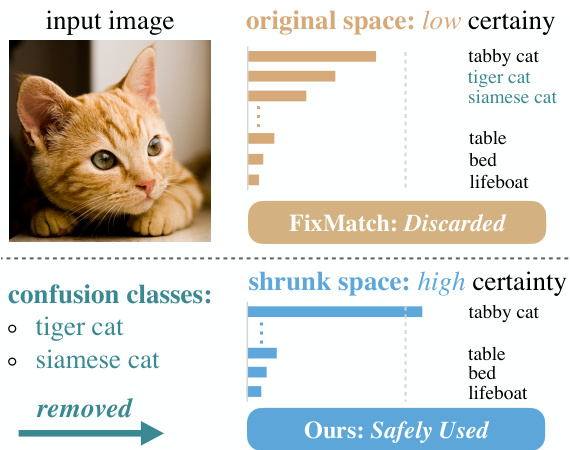
Figure 1: Illustration of our motivation. Due to confusion classes for the top-1 class, the certainty fails to reach the pre-defined threshold (gray dotted line). FixMatch discards such uncertain samples. Our method, however, detects and removes confusion classes to enhance certainty, then enjoying full and safe utilization of all unlabeled images.
图 1: 方法动机示意图。由于存在与top-1类别易混淆的类别,置信度无法达到预设阈值(灰色虚线)。FixMatch会丢弃这类不确定样本。而我们的方法通过检测并移除混淆类别来提升置信度,从而实现对所有未标注图像的安全充分利用。
So first, why are these samples uncertain? According to our observations on CIFAR-100 and ImageNet, although the top-1 accuracy could be low, the top-5 accuracy is much higher. This indicates in most cases, the model struggles to discriminate among a small portion of classes. As illustrated in Fig. 1, given a cat image, the model is not sure whether it belongs to tabby cat, tiger cat, or other cats. On the other hand, however, it is absolutely certain that the object is more like a tabby cat, rather than a table or anything else. In other words, it is reliable for the model to distinguish the top class from the remaining less likely classes.
首先,为什么这些样本存在不确定性?根据我们在CIFAR-100和ImageNet上的观察,尽管top-1准确率可能较低,但top-5准确率却高得多。这表明在大多数情况下,模型难以区分一小部分类别。如图1所示,给定一张猫的图像,模型不确定它属于虎斑猫、虎猫还是其他猫类。然而另一方面,模型可以完全确定该对象更像虎斑猫,而不是桌子或其他任何东西。换句话说,模型能够可靠地将最可能的类别与其余可能性较低的类别区分开来。
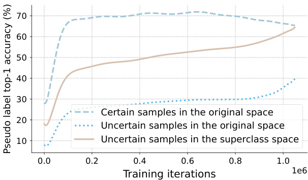
Figure 2: Pseudo label accuracy on CIFAR-100 with 400 labels. We highlight that even for uncertain samples, their top-1 predictions are of high accuracy in the superclass space (20 classes). This accuracy can even be comparable to the delicately selected certain samples in the original class space.
图 2: 在仅有400个标注的CIFAR-100数据集上的伪标签准确率。我们特别指出,即使对于不确定样本,其top-1预测在超类空间(20个类别)中也具有较高准确率,这种准确率甚至可以与原始类别空间中精心筛选的确定样本相媲美。
Invoked by these, we propose a novel method dubbed Shrink Match to learn uncertain samples. The prediction fails to satisfy the pre-defined threshold due to the existence of confusion classes for the top-1 class. Hence, our approach adaptively seeks a shrunk class space where the confusion classes are removed, to enable the re-calculated confidence to reach the original threshold. Moreover, the obtained shrunk class space is also required to be the largest among those that can satisfy the threshold. In a word, we seek a certain and largest shrunk space for uncertain samples. Then, logits of the strongly augmented image are correspondingly gathered in the new space. And a consistency regular iz ation is imposed between the shrunk weak-strong predictions.
受此启发,我们提出了一种名为Shrink Match的新方法用于学习不确定样本。由于存在与top-1类别易混淆的类别,预测结果无法满足预设阈值。因此,我们的方法自适应地寻找一个去除混淆类别的收缩类别空间,使得重新计算的置信度能够达到原始阈值。此外,所获得的收缩类别空间还需在满足阈值的条件下尽可能大。简言之,我们为不确定样本寻找一个确定且最大的收缩空间。随后,强增强图像的对数概率将在新空间中进行相应聚合,并在收缩后的强弱预测之间施加一致性正则化约束。
Note that, the confusion classes are detected and removed in a fully automatic and instance-adaptive fashion. Moreover, even if the predicted top-1 class is not fully in line with the ground truth label, they mostly belong to the same superclass. To prove this, as shown in Fig. 2, uncertain samples exhibit much higher pseudo label accuracy in the superclass space than the original space. This accuracy is even comparable to that of certain samples in the original class space. Therefore, contrasting these ground truth-related classes against remaining unlikely classes is still highly beneficial, yielding more disc rim i native representations of our model. To avoid affecting the main classifier, we further adopt an auxiliary classifier to disentangle the learning in the shrunk space.
需要注意的是,混淆类别的检测和移除是完全自动且实例自适应的。此外,即使预测的top-1类别与真实标签不完全一致,它们大多属于相同的超类。如图2所示,不确定样本在超类空间中展现的伪标签准确率远高于原始空间,甚至可与原始类别空间中确定样本的准确率相媲美。因此,将这些与真实标签相关的类别与剩余不太可能的类别进行对比仍然非常有益,能为模型生成更具判别性的表征。为避免影响主分类器,我们进一步采用辅助分类器来解耦收缩空间中的学习过程。
Despite the effectiveness, there still exist two main drawbacks to the above optimization target. (1) First, it treats all uncertain samples equally. The truth, however, is that in the original class space, the top-1 confidence of different uncertain samples can vary dramatically. And it is clear that samples with larger confidence should be attached more importance. To this end, we propose to balance different uncertain samples by their confidence in the original space. (2) Moreover, the regular iz ation term also overlooks the gradually improved model state during training. At the start of training, there are abundant uncertain samples, but their predictions are extremely noisy, or even random. So even the highest scored class may share no relationship with the true class. Then as the training proceeds, the top classes become reliable. Considering this, we further propose to adaptively reweight the uncertain loss according to the model state. The model state is tracked and approximately estimated via performing exponential moving average on the proportion of certain samples in each mini-batch. With the two reweighting principles, the model turns out more stable, and avoids accumulating much noise from uncertain samples, especially at early training iterations.
尽管有效,上述优化目标仍存在两个主要缺点。(1) 首先,它对所有不确定样本一视同仁。然而事实上,在原始类别空间中,不同不确定样本的top-1置信度可能差异巨大。显然,置信度更高的样本应被赋予更大权重。为此,我们提出根据样本在原始空间中的置信度来平衡不同不确定样本。(2) 此外,正则化项也忽略了训练过程中模型状态的逐步改善。训练初期存在大量不确定样本,但其预测结果噪声极大甚至完全随机,此时最高分类别可能与真实类别毫无关联。随着训练推进,top类别会逐渐变得可靠。基于此,我们进一步提出根据模型状态自适应地重新加权不确定损失。通过对小批次中确定样本比例进行指数移动平均来追踪和近似估计模型状态。通过这两项加权原则,模型表现更稳定,并避免了(尤其是训练早期)从不稳定样本中累积过多噪声。
To summarize, our contributions lie in three aspects:
总结而言,我们的贡献主要体现在三个方面:
• We first point out that low certainty is typically caused by a small portion of confusion classes. To enhance the certainty, we propose to shrink the original class space by adaptively detecting and removing confusion ones for the top-1 class to turn it certain in the new space. • We manage to reweight the uncertain loss from two perspectives: the image-based varied reliability among different uncertain samples, and the model-based gradually improved state as the training proceeds. • Our proposed Shrink Match establishes new state-ofthe-art results on widely acknowledged benchmarks.
• 我们首先指出,低确定性通常由少量混淆类别引起。为提高确定性,我们提出通过自适应检测并移除top-1类别的混淆类别来收缩原始类别空间,使其在新空间中具有确定性。
• 我们从两个角度对不确定损失进行重新加权:基于图像的不同不确定样本间可靠性差异,以及基于模型的训练过程中逐步优化状态。
• 我们提出的Shrink Match方法在广泛认可的基准测试中创造了最新最优结果。
2. Related Work
2. 相关工作
Semi-supervised learning (SSL). The primary concern in SSL [19, 28, 36, 20, 25, 16, 37, 35, 41, 43, 14, 24, 29, 23, 4, 30, 11, 33, 2, 42] is to design effective constraints for unlabeled samples. Dating back to decades ago, pioneering works [19, 38] integrate unlabeled data via assigning pseudo labels to them, with the knowledge acquired from labeled data. In the era of deep learning, subsequent methods mainly follow such a boots trapping fashion, but greatly boost it with some key components. Specifically, to enhance the quality of pseudo labels, Π-model [18] and Mean Teacher [31] ensemble model predictions and model parameters respectively. Later works start to exploit the role of perturbations. During this trend, [27] proposes to apply stochastic perturbations on inputs or features, and enforce consistency across these predictions. Then, UDA [34] emphasizes the necessity of strengthening the perturbation pool. It also follows VAT [22] and MixMatch [3] to supervise the prediction under strong perturbations with that under weak perturbations. Since then, weak-to-strong consistency regular iz ation has become a standard practice in SSL. Eventually, the milestone work FixMatch [28] presents a simplified framework using a fixed confidence threshold to discard uncertain samples. Our Shrink Match is built upon FixMatch. But, we highlight the value of previously neglected uncertain samples, and leverage them in an informative but also safe manner.
半监督学习 (SSL)。SSL [19, 28, 36, 20, 25, 16, 37, 35, 41, 43, 14, 24, 29, 23, 4, 30, 11, 33, 2, 42] 的核心问题在于为未标注样本设计有效约束。早在数十年前,先驱工作 [19, 38] 就通过从标注数据中获取知识,为未标注数据分配伪标签来实现数据整合。在深度学习时代,后续方法主要延续这种自举 (bootstrapping) 范式,但通过关键组件大幅提升了性能。具体而言,为提升伪标签质量,Π-model [18] 和 Mean Teacher [31] 分别对模型预测和模型参数进行集成。后续研究开始探索扰动的作用,其中 [27] 提出对输入或特征施加随机扰动,并强制这些预测之间保持一致性。随后,UDA [34] 强调增强扰动池的必要性,并遵循 VAT [22] 和 MixMatch [3] 的思路,用弱扰动下的预测监督强扰动下的预测。自此,弱-强一致性正则化成为 SSL 的标准实践。最终,里程碑工作 FixMatch [28] 提出使用固定置信度阈值剔除不确定样本的简化框架。我们的 Shrink Match 基于 FixMatch,但强调了先前被忽略的不确定样本的价值,并以信息丰富且安全的方式加以利用。
More recently, DST [7] decouples the generation and utilization of pseudo labels with a main and an auxiliary head respectively. Besides, SimMatch [45] explores instancelevel relationships with labeled embeddings to supplement original class-level relations. Compared with them, our Shrink Match achieves larger improvements.
最近,DST [7] 通过分别使用主头和辅助头来解耦伪标签的生成和利用。此外,SimMatch [45] 利用带标签的嵌入来探索实例级关系,以补充原始的类级关系。相比之下,我们的 Shrink Match 取得了更大的改进。
Defining uncertain samples. Earlier works estimate the uncertainty with Bayesian Neural Networks [15], or its faster approximation, e.g., Monte Carlo Dropout [12]. Some other works measure the prediction disagreement among multiple randomly augmented inputs [32]. The latest trend is to directly use the entropy of predictions [39], cross entropy [36], or softmax confidence [28] as a measurement for uncertainty. Our work is not aimed at the optimal uncertainty estimation strategy, so we adopt the simplest solution from FixMatch, i.e., using the maximum softmax output as the certainty.
定义不确定样本。早期研究通过贝叶斯神经网络[15]或其快速近似方法(如蒙特卡洛Dropout[12])来估计不确定性。另一些工作则通过测量多个随机增强输入之间的预测分歧[32]进行评估。最新趋势是直接使用预测熵[39]、交叉熵[36]或softmax置信度[28]作为不确定性度量指标。本研究不追求最优不确定性估计策略,因此采用FixMatch中最简方案,即以最大softmax输出作为确定性度量。
Utilizing uncertain samples. UPS [26] leverages negative class labels whose confidence is below a pre-defined threshold, from a reversed multi-label classification perspective. In comparison, our model is enforced to tell the most likely class without being cheated by the less likely ones. So our supervision on uncertain samples is more informative and produces more disc rim i native representations. Moreover, we do not introduce any extra hyper-parameters, e.g., the lower threshold in [26], into our framework.
利用不确定样本。UPS [26] 从反向多标签分类的角度,利用了置信度低于预设阈值的负类标签。相比之下,我们的模型被强制要求识别最可能的类别,而不被可能性较低的类别所欺骗。因此,我们对不确定样本的监督信息更丰富,并能产生更具判别性的表征。此外,我们的框架没有引入任何额外的超参数(例如 [26] 中的下限阈值)。
3. Method
3. 方法
We primarily provide some notations and review a common practice in semi-supervised learning (SSL) (Sec. 3.1). Next, we present our Shrink Match in detail (Sec. 3.2 and Sec. 3.3). Finally, we summarize our approach and provide a further discussion (Sec. 3.4 and Sec. 3.5).
我们首先提供一些符号说明并回顾半监督学习(SSL)中的常见做法(第3.1节)。接着详细阐述我们的Shrink Match方法(第3.2节和第3.3节)。最后总结我们的方法并进行深入讨论(第3.4节和第3.5节)。
3.1. Preliminaries
3.1. 预备知识
$$
\mathcal{L}{u}=\frac{1}{B_{u}}\sum_{k=1}^{B_{u}}\mathbb{1}(\boldsymbol{\xi}(\boldsymbol{p}{k}^{w})\geq\boldsymbol{\tau})\cdot\mathrm{H}(\boldsymbol{p}{k}^{w},\boldsymbol{p}_{k}^{s}),
$$
$$
\mathcal{L}{u}=\frac{1}{B_{u}}\sum_{k=1}^{B_{u}}\mathbb{1}(\boldsymbol{\xi}(\boldsymbol{p}{k}^{w})\geq\boldsymbol{\tau})\cdot\mathrm{H}(\boldsymbol{p}{k}^{w},\boldsymbol{p}_{k}^{s}),
$$
pre-defined to abandon uncertain ones. So the unsupervised loss $\mathcal{L}_{u}$ can be formulated as:
预定义以舍弃不确定样本。因此无监督损失 $\mathcal{L}_{u}$ 可表示为:
Semi-supervised learning aims to learn a model with limited labeled images $\mathcal{D}^{l}={(x_{k},y_{k})}$ , aided by a large number of unlabeled images $D^{u}={u_{k}}$ . Recent frameworks commonly follow the FixMatch practice. Concretely, an unlabeled image $u$ is first transformed by a weak augmentation pool $\mathcal{A}^{w}$ and a strong augmentation pool $\mathcal{A}^{s}$ to yield a pair of weakly and strongly augmented images $(\boldsymbol{u}^{w},\boldsymbol{u}^{s})$ . Then, they are fed into the model together to produce corresponding predictions $(p^{w},p^{s})$ . Typically, $p^{w}$ is of much higher accuracy than $p^{s}$ , while $p^{s}$ is beneficial to learning. Therefore, $p^{w}$ serves as the pseudo label for $p^{s}$ . Moreover, a core practice introduced by FixMatch is that, to improve the quality of selected pseudo labels, a fixed confidence threshold is where $B^{u}$ is the batch size of unlabeled images and $\tau$ is the pre-defined threshold. $\xi(p_{k}^{w})$ computes the confidence of logits $p_{k}^{w}$ by $\xi(\cdot)=\operatorname*{max}(\sigma(\cdot))$ , where $\sigma$ is the softmax func- tion. The $\mathrm{H}$ denotes the consistency regular iz ation between the two distributions. It is typically the cross entropy loss.
半监督学习旨在利用有限的标注图像 $\mathcal{D}^{l}={(x_{k},y_{k})}$ 和大量未标注图像 $D^{u}={u_{k}}$ 学习模型。当前主流框架通常遵循FixMatch策略:首先对未标注图像 $u$ 分别进行弱增强 $\mathcal{A}^{w}$ 和强增强 $\mathcal{A}^{s}$ 处理,生成增强图像对 $(\boldsymbol{u}^{w},\boldsymbol{u}^{s})$ ,随后输入模型获得预测结果 $(p^{w},p^{s})$ 。其中 $p^{w}$ 的准确率显著高于 $p^{s}$ ,而 $p^{s}$ 有助于模型学习,因此将 $p^{w}$ 作为 $p^{s}$ 的伪标签。FixMatch的核心创新在于通过固定置信度阈值筛选高质量伪标签,公式中 $B^{u}$ 表示未标注图像的批次大小, $\tau$ 为预设阈值。置信度计算函数 $\xi(p_{k}^{w})=\operatorname*{max}(\sigma(\cdot))$ 通过对数几率 $p_{k}^{w}$ 取softmax最大值实现, $\mathrm{H}$ 表示两个分布间的一致性正则项,通常采用交叉熵损失函数。
In addition, the labeled images are learned with a regular cross entropy loss to obtain the supervised loss $\mathcal{L}_{x}$ . The overall loss in each mini-batch then will be:
此外,标注图像通过常规交叉熵损失学习以获得监督损失 $\mathcal{L}_{x}$。每个小批量的总损失为:
$$
\mathcal{L}=\mathcal{L}{x}+\lambda_{u}\cdot\mathcal{L}_{u},
$$
$$
\mathcal{L}=\mathcal{L}{x}+\lambda_{u}\cdot\mathcal{L}_{u},
$$
where $\lambda_{u}$ acts as a trade-off term between the two losses.
其中 $\lambda_{u}$ 作为两个损失函数之间的权衡项。
3.2. Shrinking the Class Space for Certainty
3.2 缩小类别空间以提高确定性
Our motivation. As reviewed above, FixMatch discards the samples whose confidence is lower than a pre-defined threshold, because their pseudo labels are empirically found relatively noisier. These samples are named uncertain samples in this work. Although this practice retains high-quality pseudo labels, it incurs a low utilization of the whole unlabeled set, especially when the scenario is challenging and the selection criterion is strict. Take the CIFAR-100 dataset as an instance, with a common threshold of 0.95 and 4 labels per class, there will be nearly $20%$ unlabeled samples being ignored due to their low certainty. We argue that, these uncertain samples can still benefit the model optimization, as long as we can design appropriate constraints (loss functions) on them. So we first investigate the cause of low certainty to gain some better intuitions.
我们的动机。如前所述,FixMatch会丢弃置信度低于预定义阈值的样本,因为经验发现它们的伪标签噪声相对较大。这些样本在本研究中被称为不确定样本。虽然这种做法保留了高质量的伪标签,但导致整个未标记集的利用率较低,尤其是在场景具有挑战性且选择标准严格的情况下。以CIFAR-100数据集为例,在常见的0.95阈值和每类4个标签的设置下,由于置信度低,近20%的未标记样本会被忽略。我们认为,只要能为这些不确定样本设计适当的约束(损失函数),它们仍能为模型优化带来益处。因此,我们首先探究低确定性的成因以获得更深入的洞见。
The reason for the low certainty of an unlabeled image is that, the model tends to be confused among some top classes. For example, given a cat image, the score of the class tabby cat and class tiger cat may be both high, so the model is not absolutely certain what the concrete class is. Motivated by this observation, we propose to shrink the original class space via adaptively detecting and removing the confusion classes for the top-1 class. Then the shrunk space is only composed of the original top-1 class, as well as the remaining less likely classes. After this process, re-calculated confidence of the top-1 class will satisfy the pre-defined threshold. Thereby, we can enforce the model to learn the previously uncertain samples in this new certain space, as shown in Fig. 3. Following the previous cat example, if the top-1 class is tabby cat, our method will scan scores of all other classes, and remove confusion ones (e.g., tiger cat and siamese cat) to construct a confident shrunk space, where the model is sure that the image is a tabby cat, rather than a table. Since we do not ask the model to discriminate among several top classes, it will avoid suffering from the noise when it makes a wrong judgment in the original space.
未标注图像确定性低的原因在于,模型容易在某些头部类别间产生混淆。例如给定一张猫的图像,虎斑猫类别与虎猫类别的得分可能都很高,导致模型无法完全确定具体类别。基于这一观察,我们提出通过自适应检测并剔除与top-1类别易混淆的类别,从而收缩原始类别空间。收缩后的空间仅包含原始top-1类别及剩余低概率类别。经过此处理后,重新计算的top-1类别置信度将满足预设阈值。如图3所示,该方法可强制模型在新构建的确定性空间中学习先前不确定的样本。以前述猫的示例为例,若top-1类别为虎斑猫,本方法会扫描所有其他类别的得分,并移除混淆类别(如虎猫和暹罗猫)以构建确信的收缩空间——此时模型能确定图像是虎斑猫而非桌子。由于不再要求模型区分多个头部类别,可避免其在原始空间做出错误判断时产生的噪声干扰。
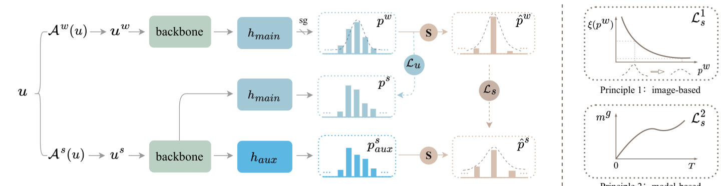
Principle 2:model-based Figure 3: An overview of our proposed Shrink Match. Our motivation is to fully leverage the originally uncertain samples. “S” denotes shrinking the class space. The confusion classes for the top-1 class are detected and removed in a fully automatic and instance-adaptive fashion, to construct a shrunk space where the top-1 class is turned certain. $\mathcal{L}{u}$ is the original certain loss, while $\mathcal{L}{s}$ calculates the uncertain loss in the shrunk class space. We add an auxiliary head $h_{a u x}$ to learn in the new space. On the right, we further reweight $\mathcal{L}_{s}$ based on two principles. Principle 1 (image-based): image predictions with larger reliability are attached more importance. Principle 2 (model-based): We track the model state during training for re weighting.
图 3: 我们提出的Shrink Match方法概览。我们的动机是充分利用原始不确定样本。"S"表示收缩类别空间。通过全自动且实例自适应的方式检测并移除与top-1类别易混淆的类别,构建一个使top-1类别转为确定的收缩空间。$\mathcal{L}{u}$是原始确定损失,而$\mathcal{L}{s}$计算收缩类别空间中的不确定损失。我们添加辅助头$h_{aux}$在新空间中进行学习。右侧我们基于两个原则对$\mathcal{L}_{s}$进行重新加权。原则1(基于图像):可靠性更高的图像预测被赋予更大权重。原则2(基于模型):我们在训练过程中跟踪模型状态进行重新加权。
How to seek the shrunk class space? Now, how can we enable our method to automatically seek the optimal shrunk space of an uncertain unlabeled image? Ideally, we hope this seeking process is free from any prior knowledge from humans, e.g., class relationships, and also does not require any extra hyper-parameters. Considering these, we opt to inherit the pre-defined confidence threshold as a criterion. To be specific, we first sort the predicted logits in a descending order to obtain $p^{w}={s_{n_{i}}^{w}}_{i=1}^{C}$ for classes ${n_{i}}_{i=1}^{C}$ , where snwi ≥ snwi+1. In the shrunk space, we will retain the original top-1 class, because it is still the most likely one to be true. Then, we find a set of less likely classes ${n_{i}}_{i=K}^{C}$ by enforcing two constraints on the $K$ :
如何寻找收缩后的类别空间?现在,我们如何让方法自动为不确定的未标注图像寻找最优的收缩空间?理想情况下,我们希望这一寻找过程无需依赖任何人类先验知识(例如类别关系),也不引入额外超参数。基于此,我们选择沿用预定义的置信度阈值作为判断标准。具体而言,我们首先对预测logits进行降序排序,得到类别${n_{i}}_{i=1}^{C}$对应的$p^{w}={s_{n_{i}}^{w}}_{i=1}^{C}$,其中$s_{n_{i}}^{w} \geq s_{n_{i+1}}^{w}$。在收缩空间中,我们将保留原始top-1类别,因为它仍是最可能正确的类别。接着,通过对$K$施加两个约束条件,找到一组可能性较低的类别${n_{i}}_{i=K}^{C}$:
$$
\begin{array}{r l}&{\xi({s_{n_{1}}^{w}}\cup{s_{n_{i}}^{w}}{i=K}^{C})\geq\tau,}\ &{\xi({s_{n_{1}}^{w}}\cup{s_{n_{i}}^{w}}_{i=K-1}^{C})<\tau,}\end{array}
$$
$$
\begin{array}{r l}&{\xi({s_{n_{1}}^{w}}\cup{s_{n_{i}}^{w}}{i=K}^{C})\geq\tau,}\ &{\xi({s_{n_{1}}^{w}}\cup{s_{n_{i}}^{w}}_{i=K-1}^{C})<\tau,}\end{array}
$$
where $\xi$ is defined the same as that in Eq. (1), calculating the icso nc of id mep nocs e eodf tohf et rhee- arses-e as ms bel med b lleodg itcsl.a sTshees ${n_{1}}\cup{n_{i}}_{i=K}^{C}$ The two constraints on not only ensure the top-1 class is turned certain in the new space (Eq. (3)), but also select the largest space among all candidates (Eq. (4)).
其中 $\xi$ 的定义与式 (1) 相同,计算 icso nc of id mep nocs e eodf tohf et rhee-arses-e as ms bel med b lleodg itcsl.a sTshees ${n_{1}}\cup{n_{i}}_{i=K}^{C}$。这两个约束条件不仅确保 top-1 类别在新空间中变为确定状态 (式 (3)),同时还从所有候选空间中选择最大的空间 (式 (4))。
How to learn in the shrunk class space? For a weakly augmented uncertain image $x^{w}$ , the model is certain about its top-1 class in the shrunk class space. To learn effectively in this space, we follow the popular practice of weak-to-strong consistency regular iz ation. The correspondingly shrunk prediction on the strongly augmented image is enforced to match that on the weakly augmented one. Concretely, for clarity, the re-assembled logits from $p^{w}$ is denoted as $\hat{p}^{w}$ , which means $\hat{p}^{w}={s_{n_{1}}^{w}}\cup{s_{n_{i}}^{w}}{K}^{C}$ . We use the re-assembled classes ${n_{1}}\cup{n_{i}}{K}^{C}$ in the shrunk space to correspondingly gather the logits $p^{s}$ on $x^{s}$ , yielding $\hat{p}^{s}={s_{n_{1}}^{s}}\cup{s_{n_{i}}^{s}}_{K}^{C}$ . Then we can regularize the consistency between the two shrunk distributions $\hat{p}^{s}$ and $\hat{p}^{w}$ , similar to that in Eq. (1):
如何在缩小的类别空间中学习?对于弱增强的不确定图像$x^{w}$,模型对其在缩小类别空间中的top-1类别是确定的。为了在该空间中有效学习,我们遵循弱到强一致性正则化的流行做法。强制要求强增强图像上的相应缩小预测与弱增强图像上的预测相匹配。具体来说,为清晰起见,从$p^{w}$重新组装的logits记为$\hat{p}^{w}$,即$\hat{p}^{w}={s_{n_{1}}^{w}}\cup{s_{n_{i}}^{w}}{K}^{C}$。我们使用缩小空间中的重新组装类别${n_{1}}\cup{n_{i}}{K}^{C}$来相应收集$x^{s}$上的logits$p^{s}$,得到$\hat{p}^{s}={s_{n_{1}}^{s}}\cup{s_{n_{i}}^{s}}_{K}^{C}$。然后可以正则化两个缩小分布$\hat{p}^{s}$和$\hat{p}^{w}$之间的一致性,类似于式(1)中的做法:
$$
\mathcal{L}{s}=\frac{1}{B_{u}}\sum_{k=1}^{B_{u}}\mathbb{1}(\boldsymbol{\xi}(\boldsymbol{p}{k}^{w})<\boldsymbol{\tau})\cdot\hat{\mathrm{H}}(\hat{\boldsymbol{p}}{k}^{w},\hat{\boldsymbol{p}}_{k}^{s}),
$$
$$
\mathcal{L}{s}=\frac{1}{B_{u}}\sum_{k=1}^{B_{u}}\mathbb{1}(\boldsymbol{\xi}(\boldsymbol{p}{k}^{w})<\boldsymbol{\tau})\cdot\hat{\mathrm{H}}(\hat{\boldsymbol{p}}{k}^{w},\hat{\boldsymbol{p}}_{k}^{s}),
$$
where the indicator function is to find uncertain samples.
指示函数用于寻找不确定样本。
Empirically, we observe that if we use the original linear head $h_{m a i n}$ to learn this auxiliary supervision, it will make the confidence of our model increase aggressively. Most noisy unlabeled samples are blindly judged as certain ones. We conjecture that it is because the $\mathcal{L}{s}$ strengthens weights of the classes that are frequently uncertain, then these classes will be incorrectly turned certain. With this in mind, our solution is simple. We adopt an auxiliary MLP head $h_{a u x}$ that shares the backbone with $h_{m a i n}$ , to deal with this auxiliary optimization target, as shown in Fig. 3. So the $\hat{p}^{s}$ is indeed gathered from predictions of $h_{a u x}$ ( $\hat{p}^{w}$ is still from $h_{m a i n.}$ ). This modification enables our feature extractor to acquire more disc rim i native representations, and meantime does not affect predictions of the main head. Note that $h_{a u x}$ is only applied for training, bringing no burden to the test stage.
根据实验观察,若使用原始线性头 $h_{main}$ 学习该辅助监督任务,会导致模型置信度急剧上升,大量含噪声的未标注样本被盲目判定为确定样本。我们推测这是由于 $\mathcal{L}{s}$ 强化了频繁处于不确定状态的类别权重,致使这些类别被错误地转为确定状态。为此,我们提出一种简单解决方案:如图3所示,采用与 $h_{main}$ 共享主干网络的辅助MLP头 $h_{aux}$ 来处理该辅助优化目标。此时 $\hat{p}^{s}$ 实际来自 $h_{aux}$ 的预测(而 $\hat{p}^{w}$ 仍由 $h_{main}$ 生成)。这一改进使特征提取器能获得更具判别性的表征,同时不影响主头的预测性能。需注意 $h_{aux}$ 仅用于训练阶段,不会增加测试时的计算负担。
3.3. Re weighting the Uncertain Loss
3.3. 不确定性损失重加权
Despite the effectiveness of the above uncertain loss, there still exist two main drawbacks. (1) On one hand, it overlooks the varied reliability of the top-1 class among different uncertain images. For example, suppose two uncertain images $u_{1}$ and $u_{2}$ with softmax predictions [0.8, 0.1, 0.1] and [0.5, 0.3, 0.2] in the original space, they should not be treated equally in the shrunk space. The $u_{1}$ with top-1 confidence of 0.8 is more likely to be true than $u_{2}$ , and thereby should be attached more attention to. (2) On the other, it ignores the gradually improved model performance as the training proceeds. To be concrete, at the very start of training, the predictions are extremely noisy or even random. And then at later stages, the predictions become more and more reliable. So the uncertain predictions at different training stages should not be treated equally. Therefore, we further design two re weighting principles for the two concerns.
尽管上述不确定性损失方法有效,但仍存在两个主要缺陷:(1) 一方面,它忽略了不同不确定图像中top-1类别的可靠性差异。例如,假设原始空间中两个不确定图像$u_{1}$和$u_{2}$的softmax预测值分别为[0.8, 0.1, 0.1]和[0.5, 0.3, 0.2],它们在压缩空间中不应被同等对待。top-1置信度为0.8的$u_{1}$比$u_{2}$更可能为真,因此应获得更多关注。(2) 另一方面,它忽略了模型性能随训练进程逐步提升的特性。具体而言,训练初期的预测噪声极大甚至随机,而后期预测会越来越可靠。因此,不同训练阶段的不确定性预测不应被等同视之。基于这两个考量,我们进一步设计了两项重加权原则。
Principle 1: Re weighting with image-based varied reliability. According to the above intuition, we directly reweight the uncertain loss of each uncertain image by its top-1 confidence $\xi(p_{k}^{w})$ in the original class space, which is:
原则1: 基于图像可变可靠性的重加权。根据上述直觉,我们直接通过每张不确定图像在原类别空间中的top-1置信度$\xi(p_{k}^{w})$对其不确定损失进行重加权,即:
$$
\mathcal{L}{s}^{1}=\frac{1}{B_{u}}\sum_{k=1}^{B_{u}}\mathbb{1}(\xi(p_{k}^{w})<\tau)\cdot\hat{\mathrm{H}}(\hat{p}{k}^{w},\hat{p}_{k}^{s})\cdot\xi(p_{k}^{w}).
$$
$$
\mathcal{L}{s}^{1}=\frac{1}{B_{u}}\sum_{k=1}^{B_{u}}\mathbb{1}(\xi(p_{k}^{w})<\tau)\cdot\hat{\mathrm{H}}(\hat{p}{k}^{w},\hat{p}{k}^{s})\cdot\xi(p_{k}^{w}).
$$
We do not use the top-1 confidence $\xi(\hat{p}{k}^{w})$ in the shrunk space as the weight, because after shrinking, this value of different predictions is very close to each other. So generally, $\xi(p_{k}^{w})$ is more disc rim i native than $\xi(\hat{p}_{k}^{w})$ as the weight.
我们不以收缩空间中的最高置信度 $\xi(\hat{p}{k}^{w})$ 作为权重,因为收缩后不同预测的该值彼此非常接近。因此,通常 $\xi(p_{k}^{w})$ 比 $\xi(\hat{p}_{k}^{w})$ 更具区分性,更适合作为权重。
Principle 2: Re weighting with model-based gradually improved state. One naïve solution is to linearly increase the loss weight of $\mathcal{L}_{s}$ from 0 at the beginning to $\mu$ at iteration $T$ , and then keep $\mu$ until the end. However, this practice has two severe disadvantages. First, the two additional hyperparameters $\mu$ and $T$ are not easy to determine, and could be sensitive. More importantly, the linear scheduling criterion simply assumes the model state also improves linearly. Indeed, it can not be true. Thus, we here present a more promising principle to perform re weighting, that is free from any extra hyper-parameters. It can adjust the loss weight according to the model state in a fully adaptive fashion. To be specific, we use the certain ratio of the unlabeled set as an indicator for the model state. The certain ratio is traced at each iteration and accumulated globally in an exponential moving average (EMA) manner. Formally, the certain ratio in a single mini-batch is given by:
原则2:基于模型状态渐进改善的重新加权。一种简单的方法是从初始阶段将$\mathcal{L}_{s}$的损失权重从0线性增加到迭代$T$时的$\mu$,之后保持$\mu$直至训练结束。但这种方法存在两个明显缺陷:首先,额外超参数$\mu$和$T$难以确定且可能敏感;更重要的是,线性调度假设模型状态也呈线性改善,这往往不符合实际。因此,我们提出一种无需额外超参数、能根据模型状态自适应调整损失权重的优化方案。具体而言,我们使用未标注数据集的确定比例作为模型状态指标,该比例通过指数移动平均(EMA)方式在每次迭代时追踪并全局累积。单批次训练中的确定比例计算公式为:
$$
m=\frac{1}{B_{u}}\sum_{k=1}^{B_{u}}\mathbb{1}(\xi(p_{k}^{w})\geq\tau).
$$
$$
m=\frac{1}{B_{u}}\sum_{k=1}^{B_{u}}\mathbb{1}(\xi(p_{k}^{w})\geq\tau).
$$
The global certain ratio $m^{g}$ is initialized as 0, and accumulated at each training iteration by:
全局确定比率 $m^{g}$ 初始化为0,并通过以下方式在每个训练迭代中累积:
$$
m^{g}\gets\gamma\cdot m^{g}+(1-\gamma)\cdot m,
$$
$$
m^{g}\gets\gamma\cdot m^{g}+(1-\gamma)\cdot m,
$$
where $\gamma$ is the momentum coefficient. It is a hyper-parameter already defined in FixMatch (baseline), where it is used to update the teacher parameters for final evaluation.
其中$\gamma$是动量系数。该超参数已在FixMatch (基线方法)中定义,用于更新教师模型的参数以进行最终评估。
Obviously, $m^{g}$ falls between 0 and 1. And it will approximately increase from 0 to a nearly saturated value. Then, the reweighted uncertain loss is given by:
显然,$m^{g}$ 介于0到1之间,并将近似从0递增至接近饱和值。于是,重加权不确定损失由下式给出:
$$
\mathcal{L}{s}^{2}=m^{g}\cdot\frac{1}{B_{u}}\sum_{k=1}^{B_{u}}\mathbb{1}(\xi(p_{k}^{w})<\tau)\cdot\hat{\mathrm{H}}(\hat{p}{k}^{w},\hat{p}_{k}^{s}).
$$
$$
\mathcal{L}{s}^{2}=m^{g}\cdot\frac{1}{B_{u}}\sum_{k=1}^{B_{u}}\mathbb{1}(\xi(p_{k}^{w})<\tau)\cdot\hat{\mathrm{H}}(\hat{p}{k}^{w},\hat{p}_{k}^{s}).
$$
Integrating the above two intuitions and principles, the final reweighted uncertain loss will be:
综合上述两种直觉和原则,最终重新加权的损失函数为:
$$
\mathcal{L}{s}=m^{g}\cdot\frac{1}{B_{u}}\sum_{k=1}^{B_{u}}\mathbb{1}(\xi(p_{k}^{w})<\tau)\cdot\hat{\mathbf{H}}(\hat{p}{k}^{w},\hat{p}{k}^{s})\cdot\xi(p_{k}^{w}).
$$
$$
\mathcal{L}{s}=m^{g}\cdot\frac{1}{B_{u}}\sum_{k=1}^{B_{u}}\mathbb{1}(\xi(p_{k}^{w})<\tau)\cdot\hat{\mathbf{H}}(\hat{p}{k}^{w},\hat{p}{k}^{s})\cdot\xi(p_{k}^{w}).
$$
3.4. Summary
3.4. 总结
To summarize, the final loss in a mini-batch is a combination of the supervised loss $(\mathcal{L}{x})$ , certain loss ( $\mathcal{L}{u}$ , Eq. (1)), and uncertain loss in the shrunk class space ( $\mathcal{L}_{s}$ , Eq. (10)):
综上所述,小批量(mini-batch)的最终损失是监督损失 $(\mathcal{L}{x})$ 、确定性损失 ( $\mathcal{L}{u}$ ,式(1)) 以及收缩类别空间中的不确定性损失 ( $\mathcal{L}_{s}$ ,式(10)) 的组合:
$$
\mathcal{L}=\mathcal{L}{x}+\lambda_{u}\cdot(\mathcal{L}{u}+\mathcal{L}_{s}).
$$
$$
\mathcal{L}=\mathcal{L}{x}+\lambda_{u}\cdot(\mathcal{L}{u}+\mathcal{L}_{s}).
$$
We do not carefully fine-tune the fusion weight between $\mathcal{L}{u}$ and $\mathcal{L}_{s}$ , but use 1:1 by default to avoid hyper-parameters.
我们没有仔细微调 $\mathcal{L}{u}$ 和 $\mathcal{L}_{s}$ 之间的融合权重,而是默认使用 1:1 的比例以避免超参数调整。
3.5. Discussions
3.5. 讨论
Our uncertain loss in the shrunk space owns two properties: informative and also safe. The first property is because we manage to find the largest shrunk space that reaches the confidence threshold. Besides, we also adopt the weak-tostrong consistency regular iz ation to pose a challenging optimization target. Both constraints ensure the learning in the shrunk space is not trivial and still quite informative. Next, we wish to explain the second property “safe”, especially about how we avoid noise in the shrunk space.
我们在收缩空间中的不确定性损失具有两个特性:信息丰富且安全。第一个特性源于我们成功找到了达到置信度阈值的最大收缩空间。此外,我们还采用了弱到强一致性正则化来设定具有挑战性的优化目标。这两项约束确保了收缩空间内的学习并非琐碎,仍具有丰富信息量。接着,我们将解释第二个特性"安全",特别是关于如何避免收缩空间中的噪声。
Noises in pseudo labels distinguish the semi-supervised paradigm from the fully-supervised one. So designing a safe optimization target for unlabeled data is crucial. Typically, the cross entropy loss will maximize the softmax probability $\exp{(s_{t})}/{\sum_{i=1}^{\infty}\exp(s_{i})}\rightarrow1$ for the target class $t$ . It inevitably su ppresses scores of all other classes except $t$ However, the true class could not be $t$ , and may be the $2^{\mathrm{nd}}$ or $3^{\mathrm{rd}}$ largest class, etc., which is wrongly restrained. This is frequently observed when the confidence of class $t$ is not high enough. As a milder alternative, the soft labeling still encounters a similar problem. In contrast, our shrunk target directly excludes these confusion classes. So only the almost unlikely classes are suppressed.
伪标签中的噪声将半监督范式与全监督范式区分开来。因此为未标记数据设计安全的优化目标至关重要。典型的交叉熵损失会使目标类 $t$ 的softmax概率 $\exp{(s_{t})}/{\sum_{i=1}^{\infty}\exp(s_{i})}\rightarrow1$ 最大化,这不可避免地会抑制除 $t$ 之外所有其他类的得分。然而真实类别可能并非 $t$,而可能是第 $2^{\mathrm{nd}}$ 或第 $3^{\mathrm{rd}}$ 大类别等,这些类别被错误地压制了——当类别 $t$ 的置信度不够高时,这种现象经常出现。作为更温和的替代方案,软标签仍会遇到类似问题。相比之下,我们的收缩目标直接排除了这些混淆类别,因此仅压制几乎不可能的类别。
It is worth noting, even if the predicted top-1 class is not in line with the human label, it is probably one of the closest semantics, e.g., belonging to the same superclass as the ground truth label, as shown in Fig. 2. Thus, contrasting these relevant classes against other less likely classes with our noise-robust shrunk loss is still beneficial. The model is encouraged to make disc rim i native predictions closer to top classes compared to tail classes. In addition, our disentangled auxiliary head can effectively leverage such supervision while not affecting the main classification tasks [7].
值得注意的是,即使预测的top-1类别与人工标注不符,它也很可能是语义最接近的类别之一(例如与真实标签同属一个上级类别),如图2所示。因此,使用我们的抗噪收缩损失函数对比这些相关类别与其他低概率类别仍然有益。该机制促使模型在预测时,使头部类别与尾部类别之间产生更具判别性的差异。此外,我们解耦的辅助头能有效利用此类监督信号,同时不影响主分类任务[7]。
4. Experiment
4. 实验
In this section, we first describe the implementation details of our framework. Then, we compare our Shrink Match with previous state-of-the-art methods (SOTAs) under extensive evaluation protocols. Lastly, we conduct comprehensive ablation studies on each component to validate the necessity.
在本节中,我们首先描述框架的实现细节。随后,在广泛的评估协议下将Shrink Match与先前最先进方法(SOTAs)进行对比。最后,对各组件开展全面的消融实验以验证其必要性。
Table 1: Comparison with SOTAs on CIFAR-10. The same seed ensures exactly the same data split. The 400 or 2500 denotes the number of labels.
表 1: CIFAR-10数据集上与其他SOTA方法的对比。相同种子确保完全相同的数据划分。400或2500表示标签数量。
| Seed | 0 | 1 | 2 3 | 4 | Mean |
|---|---|---|---|---|---|
| SimMatch [45] ShrinkMatchI40 | 95.34 95.09 | 95.16 94.66 | 92.63 93.76 95.12 94.78 | 95.10 94.95 | 94.39 94.92 |
| SimMatch [45] | 95.58 | 95.50 | 95.34 94.06 | 95.26 | 95.15 |
| ShrinkMatch | 250 | 95.39 | 95.44 | 95.36 94.76 | 95.35 |
Table 2: Comparison with SOTAs on CIFAR-100.
| Seed | 0 | 1 | 2 | 3 | 4 | Mean |
|---|---|---|---|---|---|---|
| SimMatch [45] ShrinkMatch|400 | 62.06 65.00 | 60.19 63.47 | 59.89 63.77 | 64.88 66.42 | 63.92 64.52 | 62.19 64.64 |
| SimMatch [45] | 74.64 | 75.19 | 74.53 | 75.03 | 75.24 | 74.93 |
| ShrinkMatch|2500 | 75.00 | 75.11 | 74.54 | 74.78 | 74.72 | 74.83 |
表 2: CIFAR-100上的SOTA方法对比。
4.1. Implementation Details
4.1. 实现细节
Baselines. We use FixMatch $^+$ distribution alignment (DA) as our baseline on all datasets except ImageNet and SVHN. On ImageNet, we build our method on SimMatch. On SVHN, we discard DA. To be more convincing, we adopt the same codebase as our compared methods.
基线方法。除ImageNet和SVHN数据集外,我们采用带分布对齐(DA)的FixMatch$^+$作为基线方法。在ImageNet上,我们的方法基于SimMatch构建。在SVHN数据集上,我们弃用了DA模块。为确保可比性,我们采用了与对比方法相同的代码库。
Hyper-parameters. Following prior arts, Wide ResNet-28- 2 [40], WRN-28-8, WRN-37-2, and WRN-28-2 are used for CIFAR-10, CIFAR-100, STL-10, and SVHN respectively. A ResNet-50 [13] is used for ImageNet. The auxiliary head $h_{a u x}$ for uncertain samples is a 3-layer MLP. On the ImageNet, we set $B_{u}=64\times5$ , but for other datasets, $B_{u}=$ $64\times7$ . The labeled batch size is 64 for all datasets. On the ImageNet, the model is trained for 400 epochs, while on the others, it is trained for $2^{20}$ iterations. The initial learning rate is set as 0.03 for all datasets with a cosine scheduler. Specially, on the ImageNet, it is warmed up for 5 epochs. The consistency regular iz ation $\mathrm{H}$ in $\mathcal{L}{u}$ on STL-10 and SVHN is a hard cross entropy (CE) loss, while on the CIFAR-10/100 and ImageNet, following the SimMatch and CoMatch [20], it is modified to a soft CE loss. The $\hat{\bf H}$ in our proposed $\mathscr{L}{s}$ is simply a hard CE loss. The weight $\lambda_{u}$ for the two unsupervised losses is set as 10 on the ImageNet and 1 on others. The confidence threshold $\tau$ is 0.7 on the ImageNet and 0.95 for others. The shared momentum coefficient $\gamma$ between our global certain ratio $m^{g}$ and the teacher parameters is 0.999. Following the common practice, the teacher model is only maintained for final evaluation.
超参数设置。遵循先前研究,分别使用Wide ResNet-28-2 [40]、WRN-28-8、WRN-37-2和WRN-28-2网络处理CIFAR-10、CIFAR-100、STL-10和SVHN数据集,ImageNet则采用ResNet-50 [13]。不确定性样本的辅助头$h_{aux}$为三层MLP结构。ImageNet设置$B_{u}=64\times5$,其他数据集设为$B_{u}=64\times7$。所有数据集的标注批次大小均为64。ImageNet训练400轮次,其他数据集训练$2^{20}$次迭代。初始学习率统一设为0.03并采用余弦调度器,其中ImageNet额外进行5轮次预热训练。STL-10和SVHN的一致性正则化$\mathrm{H}$采用硬交叉熵(CE)损失,而CIFAR-10/100和ImageNet参照SimMatch与CoMatch [20]改用软CE损失。我们提出的$\mathscr{L}{s}$中$\hat{\bf H}$采用简单硬CE损失。无监督损失权重$\lambda_{u}$在ImageNet设为10,其他数据集设为1。置信度阈值$\tau$在ImageNet取0.7,其他取0.95。全局确定比率$m^{g}$与教师参数的共享动量系数$\gamma$为0.999。按照惯例,教师模型仅用于最终评估。
4.2. CIFAR-10 and CIFAR-100
4.2. CIFAR-10 与 CIFAR-100
The CIFAR dataset is composed of 50000/10000 training/validation images of size $32\times32$ . The CIFAR-10 contains 10 balanced classes to recognize, while CIFAR-100 is much more challenging, containing 100 classes. We run our Shrink Match on five different seeds and report each result as well as the average result. On the CIFAR-10 of Tab. 1 where performance is almost saturated, we still obtain a nontrivial improvement of $0.53%$ $(94.39%\rightarrow94.92%)$ with 4 labels per class (400 labels in total). In addition, notably, as shown in Tab. 2, with only 4 labels per class on the challenging CIFAR-100, our Shrink Match remarkably outperforms SimMatch by $2.45%$ $62.19%\rightarrow64.64%)$ on average.
CIFAR数据集由50000/10000张尺寸为$32\times32$的训练/验证图像组成。CIFAR-10包含10个需要识别的平衡类别,而更具挑战性的CIFAR-100则包含100个类别。我们在五个不同随机种子下运行Shrink Match算法,分别报告各项结果及平均结果。在性能已接近饱和的CIFAR-10(见表1)中,我们仍以每类4个标注(总计400个标注)实现了$0.53%$ $(94.39%\rightarrow94.92%)$的显著提升。值得注意的是,如表2所示,在极具挑战性的CIFAR-100数据集上仅使用每类4个标注时,我们的Shrink Match算法平均以$2.45%$ $(62.19%\rightarrow64.64%)$的优势显著超越SimMatch。
Table 3: Comparison with SOTAs on STL-10.
表 3: STL-10数据集上的SOTA方法对比
| Seed | 0 | 1 | 2 | Mean |
|---|---|---|---|---|
| FixMatch[28] | 65.85 | 67.94 | 58.30 | 64.03 |
| FlexMatch[42] | 76.71 | 68.28 | 67.55 | 70.85 |
| ShrinkMatchT40 | 85.75 | 85.64 | 86.55 | 85.98 |
| FixMatch[28] | 90.91 | 88.71 | 90.94 | 90.19 |
| FlexMatch[42] | 91.35 | 92.29 | 91.66 | 91.77 |
| ShrinkMatchT250 | 91.13 | 92.43 | 91.10 | 91.55 |
Table 4: Comparison with SOTAs on SVHN.
表 4: SVHN数据集上的SOTA方法对比
| Seed | 1 | 2 | Mean | |
|---|---|---|---|---|
| FixMatch[28] | 94.53 | 96.90 | 97.14 | 96.19 |
| FlexMatch[42] | 89.19 | 89.93 | 96.32 | 91.81 |
| ShrinkMatchI40 | 97.96 | 97.81 | 96.70 | 97.49 |
| FixMatch[28] | 98.00 | 97.99 | 97.94 | 97.98 |
| FlexMatch[42] | 91.76 | 91.83 | 96.65 | 93.41 |
| ShrinkMatchT250 | 98.08 | 98.06 | 97.98 | 98.04 |
4.3. STL-10 and SVHN
4.3. STL-10 与 SVHN
The STL-10 dataset originally consists of 5K/100K/8K labeled/unlabeled/validation images. We follow FlexMatch to only select a subset of 40/250 labeled images, while the unlabeled set remains unchanged. As shown in Tab. 3, with 4 labels per class, our Shrink Match surpasses FlexMatch tremendously from $70.85%$ to $85.98%$ $(+15.13%)$ .
STL-10数据集原始包含5K/100K/8K标注/未标注/验证图像。我们遵循FlexMatch方案仅选取40/250标注图像子集,未标注集保持不变。如表3所示,在每类4标注样本条件下,我们的Shrink Match以$85.98%$大幅超越FlexMatch的$70.85%$,提升幅度达$(+15.13%)$。
The SVHN dataset is suitable to reveal the ability of different semi-supervised algorithms in the presence of class imbalance issue. As demonstrated in Tab. 4, although the performance of the original FixMatch (our baseline) has almost touched the upper bound, we still further boost it from $96.19%$ to $97.49%$ $(+1.30%)$ with 4 labels per class.
SVHN数据集适合用来揭示不同半监督算法在类别不平衡问题下的表现能力。如表 4 所示,尽管原始FixMatch(我们的基线)的性能几乎触及上限,但我们仍在使用每类4个标签的情况下将其准确率从$96.19%$提升至$97.49%$ $(+1.30%)$。
4.4. ImageNet-1K
4.4. ImageNet-1K
The ImageNet dataset is rather challenging, containing 1.28M/50K training/validation images of 1000 classes. We exactly follow the codebase of SimMatch [45]. As shown in Tab. 5, our Shrink Match further boosts previous best results on both settings of $1%$ and $10%$ labeled images.
ImageNet 数据集具有较高挑战性,包含1000个类别的128万/5万张训练/验证图像。我们完全遵循SimMatch [45] 的代码库。如表 5 所示,在标记图像比例为 $1%$ 和 $10%$ 的设置下,我们的 Shrink Match 进一步提升了此前的最佳结果。
Table 5: Accuracy $(%)$ on the ImageNet-1K with $1%$ and $10%$ labeled images. †: Reproduced in our environment.
表 5: ImageNet-1K 在 1% 和 10% 标注图像下的准确率 $(%)$ 。†: 在我们的环境中复现。
| 预训练方法 | 方法 | 训练轮数 | 参数量 (训练/测试) | Top-1 (1%) | Top-1 (10%) | Top-5 (1%) | Top-5 (10%) |
|---|---|---|---|---|---|---|---|
| SimCLRv2 [8] SwAV [6] | 800 | 34.2M/25.6M | 57.9 | 68.4 | 82.5 | 89.2 | |
| WCL [44] | Fine-tune | 800 | 30.4M/25.6M | 53.9 | 70.2 | 78.5 | 89.9 |
| 800 | 34.2M/25.6M | 65.0 | 72.0 | 86.3 | 91.2 | ||
| Fine-tune | 800 | 30.0M/25.6M | 49.8 | 66.1 | 77.2 | 87.9 | |
| MoCo v2 [9] MoCo-EMAN [5] | CoMatch [20] | 1200 | 30.0M/25.6M | 67.1 | 73.7 | 87.1 | 91.4 |
| FixMatch-EMAN [5] | 1100 | 30.0M/25.6M | 63.0 | 74.0 | 83.4 | 90.9 | |
| CoMatch [20] | 400 | 30.0M/25.6M | 66.0 | 73.6 | 86.4 | 91.6 | |
| SimMatchf [45] | 400 | 30.0M/25.6M | 67.0 | 74.1 | 86.9 | 91.5 | |
| None | ShrinkMatch | 400 | 31.8M/25.6M | 67.5 | 74.5 | 87.4 | 91.9 |

(a) Number of removed confusion classes. (b) Certain loss $\mathcal{L}{u}$ and uncertain loss $\mathcal{L}_{s}$ .
(a) 移除的混淆类别数量。 (b) 确定性损失 $\mathcal{L}{u}$ 和不确定性损失 $\mathcal{L}_{s}$。
(c) Ratio of uncertain samples.
(c) 不确定样本比例。
Figure 4: (a) The number of removed confusion classes for each uncertain image as the training proceeds. (b) Value of different loss functions, i.e., Eq. (1), Eq. (6), and Eq. (10). (c) The ratio of uncertain samples (certainty $<\tau$ ) in each mini-batch.
Table 6: Ablation studies of Shrink Match on CIFAR-100.
图 4: (a) 训练过程中每张不确定图像移除的混淆类别数量。(b) 不同损失函数的值,即式(1)、式(6)和式(10)。(c) 每个小批量中不确定样本(确定性$<\tau$)的占比。
| Seed | — 0 | 1 | 2 | 3 | 4 | Mean |
|---|---|---|---|---|---|---|
| Baseline | 64.40 | 57.51 | 63.07 | 64.77 | 62.53 | 62.46 |
| ShrinkMatch | 65.00 | 63.47 | 63.77 | 66.42 | 64.52 | 64.64 |
表 6: Shrink Match在CIFAR-100上的消融研究。
4.5. Ablation Studies
4.5. 消融实验
Unless otherwise specified, we conduct our ablation studies on CIFAR-100 with 4 labels per class.
除非另有说明,我们在CIFAR-100数据集上进行了消融实验,每类使用4个标签。
Effectiveness of our holistic Shrink Match. We first view our Shrink Match as a holistic component added to our baseline. As displayed in Tab. 6 for CIFAR-100, our Shrink Match boosts the strong baseline significantly by $2.18%$ $(62.46%$ $\rightarrow64.64%$ ). And on the STL-10 of Tab. 7, the baseline is also improved evidently from $84.85%$ to $85.98%$ $(+1.13%)$ .
我们整体性Shrink Match的有效性。首先将Shrink Match视为添加到基线的整体组件。如表6所示,在CIFAR-100上,我们的Shrink Match将强基线显著提升了2.18% (62.46% → 64.64%)。在表7的STL-10上,基线也从84.85%明显提升至85.98% (+1.13%)。
Effectiveness of two re weighting principles. In Sec. 3.3, considering the varied prediction reliability of different uncertain samples and different training stages, we propose two principles to reweight our uncertain loss $\mathcal{L}_{s}$ . So here we carefully examine their necessity in Tab. 8. It can be observed that the two principles are both beneficial, jointly improving the basic shrinking practice from $63.16%$ to $64.24%$ . We also attempt a simple alternative of linearly increasing the uncertain loss weight from 0 (start) to 1 (end). But as evidenced in the Exp 3 & 4 of Tab. 8, it is obviously inferior to our designed re weighting strategy. We visualize our $m^{g}$ as training proceeds on ImageNet in Fig. 5. It looks essentially different from linear scheduling. Moreover, we visualize the uncertain loss value with or without the second re weighting principle in Fig. 4b. After re weighting, the uncertain loss is of a similar magnitude as the certain loss, which can avoid dominating the gradient at early training stages.
两种重新加权原则的有效性。在3.3节中,考虑到不同不确定样本和不同训练阶段的预测可靠性差异,我们提出了两个原则来重新加权不确定损失 $\mathcal{L}_{s}$ 。因此在表8中我们仔细检验了它们的必要性。可以观察到这两个原则都是有益的,共同将基础收缩实践的准确率从 $63.16%$ 提升至 $64.24%$ 。我们还尝试了线性增加不确定损失权重(从0开始到1结束)的简单替代方案。但如表8实验3和4所示,它明显不如我们设计的重新加权策略。在图5中,我们可视化了ImageNet训练过程中 $m^{g}$ 的变化情况,其本质上与线性调度不同。此外,在图4b中我们对比了是否采用第二个重新加权原则时不确定损失值的变化。经过重新加权后,不确定损失与确定损失的数值量级相近,可以避免在训练早期阶段主导梯度更新。
Table 7: Ablation studies of Shrink Match on STL-10.
| Seed | 0 | 1 | 2 | Mean |
|---|---|---|---|---|
| Baseline | 84.86 | 84.21 | 85.47 | 84.85 |
| ShrinkMatch | 85.75 | 85.64 | 86.55 | 85.98 |
表 7: ShrinkMatch在STL-10上的消融研究。
The number of removed confusion classes. As introduced before, our approach detects and removes the confusion classes for the top-1 class in a fully automatic and instanceadaptive fashion. So we visualize the number of removed confusion classes for each uncertain sample in Fig. 4a. At the very start of training, model predictions are almost uniform, so abundant classes are removed for an uncertain sample. But as the training proceeds, much fewer confusion classes need to be removed to form a confident shrunk class space.
移除的混淆类别数量。如前所述,我们的方法以全自动且实例自适应的方式检测并移除top-1类别的混淆类别。因此我们在图4a中可视化了每个不确定样本的移除混淆类别数量。在训练初期,模型预测几乎呈均匀分布,因此会为不确定样本移除大量类别。但随着训练进行,只需移除少量混淆类别即可形成置信的收缩类别空间。
Hard label or soft label in the shrunk class space? By default, we use the hard label in the shrunk space, following FixMatch. But we also ablate the choice of using the soft label as supervision. As shown in Exp 2 & 3 of Tab. 9, the hard label is much better than the soft label. We conjecture that this is because we have shrunk the class space to a safe one. The soft label will incur some unnecessary noise.
在缩减类别空间中使用硬标签还是软标签?默认情况下,我们遵循FixMatch的做法,在缩减空间中使用硬标签。但我们也对使用软标签作为监督的选择进行了消融实验。如表9中实验2和3所示,硬标签明显优于软标签。我们推测这是因为我们将类别空间缩减到了一个安全的范围内,而软标签会引入一些不必要的噪声。
Table 8: Ablation studies on the effectiveness of the two re weighting principles. Due to randomness, the “Mean” results are more convincing. LS is short for linear scheduling, which linearly increases the loss weight.
表 8: 两种重新加权原则有效性的消融研究。由于随机性,"Mean"结果更具说服力。LS是线性调度(linear scheduling)的缩写,表示线性增加损失权重。
| Exp | Principle 1 | Principle 2 LS | Seed O | Seed 1 | Mean |
|---|---|---|---|---|---|
| 1 | 65.62 | 60.70 | 63.16 | ||
| 2 | 65.68 | 62.08 | 63.88 | ||
| 3 | 65.09 | 62.90 | 64.00 | ||
| 4 | 63.01 | 59.45 | 61.23 | ||
| 5 | √ | 65.00 | 63.47 | 64.24 |
Table 9: Ablation studies on different options to learn uncertain sample. (1) whether to shrink the class space (Shrink), (2) whether to use an auxiliary head (Aux Head), and (3) use hard $(\mathbf{H})$ or soft label (S). Exp 1 is our baseline without using uncertain images. Exp 8 & 9 are experiments of directly learning uncertain samples, which are quite noisy.
表 9: 不同不确定性样本学习方案的消融研究。(1) 是否缩减类别空间 (Shrink), (2) 是否使用辅助头 (Aux Head), (3) 使用硬标签 $(\mathbf{H})$ 或软标签 (S)。实验1是不使用不确定性图像的基线。实验8和9是直接学习噪声较大的不确定性样本的实验。
| 实验 | Shrink | AuxHead Label | Seed O | Seed 1 | Mean |
|---|---|---|---|---|---|
| 1 | Our Strong Baseline | 64.40 | 57.51 | 60.96 | |
| 2 | 65.00 | 63.47 | 64.24 | ||
| 3 | 62.92 | 59.76 | 61.34 | ||
| 4 | H | 62.43 | 58.86 | 60.65 | |
| 5 | S | 60.92 | 60.22 | 60.57 | |
| 6 | H | 64.21 | 59.17 | 61.69 | |
| 7 | S | 64.75 | 60.89 | 62.82 | |
| 8 | H | 52.90 | 51.88 | 52.39 | |
| 9 | S | 54.10 | 55.75 | 54.93 |
Effects of the auxiliary head. To prevent the main classifier from being affected, we use an auxiliary head to learn the uncertain samples in the shrunk class space only for discriminative representations. So we first provide the results when still using the main head for the shrunk space. As shown in Exp 2 & 4 of Tab. 9, the auxiliary head is indispensable for our shrinking practice. So we continue to figure out whether the improvement of our Shrink Match merely comes from the auxiliary head. We attempt to use the auxiliary head to directly learn the uncertain samples in the original space without shrinking. It can be concluded from Exp 2 & 6 & 7 of Tab. 9, the original space is indeed much inferior to our shrunk space for uncertain samples, although the auxiliary head still helps the baseline to some extent. Lastly, in Tab. 9, we also include two additional results for readers, i.e., directly learning uncertain samples without shrinking or auxiliary head (Exp 8 & 9), which are quite terrible because of introducing the abundant noise to our main classifier.
辅助头的影响。为防止主分类器受到影响,我们使用辅助头仅在收缩后的类别空间中学习不确定样本以获得判别性表征。因此我们首先展示了仍在收缩空间中使用主头的结果。如表9中实验2和4所示,辅助头对我们的收缩实践不可或缺。接着我们探究Shrink Match的改进是否仅源于辅助头。我们尝试让辅助头直接在原始空间中学习未收缩的不确定样本。从表9中实验2、6和7可以得出结论:尽管辅助头对基线仍有帮助,但原始空间确实远逊于我们收缩后的空间来处理不确定样本。最后在表9中,我们还为读者提供了两项额外结果:既不收缩也不使用辅助头直接学习不确定样本(实验8和9),由于向主分类器引入了大量噪声,这些结果相当糟糕。

Figure 5: Visualization of our global certain ratio $m^{g}$ . Table 10: Ablation studies of the confidence threshold.
图 5: 我们的全局确定比率 $m^{g}$ 的可视化。表 10: 置信度阈值的消融研究。
| Threshold | 0.98 | 0.95 | 0.90 | 0.80 | 0.70 |
|---|---|---|---|---|---|
| ShrinkMatch | 65.80 | 65.00 | 64.55 | 62.74 | 59.58 |
The ratio of uncertain samples. To further justify our motivation, in Fig. 4c, we display the ratio of uncertain samples in each mini-batch. It can be seen that even in the middle of the whole training course, there are still around $40%$ and $30%$ uncertain samples on ImageNet and CIFAR100 respectively. Therefore, an appropriate approach to utilizing these samples is necessary and definitely beneficial.
不确定样本的比例。为了进一步验证我们的动机,在图4c中,我们展示了每个小批次中不确定样本的比例。可以看出,即使在整个训练过程的中期,ImageNet和CIFAR100上仍分别存在约$40%$和$30%$的不确定样本。因此,采用适当的方法利用这些样本是必要且绝对有益的。
Different confidence thresholds $\tau$ . We also try different thresholds for uncertain samples, as shown in Tab. 10. When increasing $\tau$ from widely adopted 0.95 to 0.98 (more uncertain samples), our Shrink Match can be further improved. These results clearly highlight the effective and safe utilization of uncertain samples with our Shrink Match.
不同置信度阈值 $\tau$。我们还尝试了对不确定样本采用不同阈值,如表 10 所示。当将 $\tau$ 从广泛采用的 0.95 提高到 0.98(产生更多不确定样本)时,我们的 Shrink Match 方法能获得进一步提升。这些结果清晰表明 Shrink Match 能有效且安全地利用不确定样本。
5. Conclusion
5. 结论
In this work, we aim to fully leverage the uncertain samples in semi-supervised learning. We point out that the low certainty is typically caused by a small portion of confusion classes. Invoked by this, we propose a novel method dubbed Shrink Match to automatically detect and remove the confusion classes to construct a shrunk class space, where the top-1 class is turned certain. A weak-to-strong consistency regular iz ation is enforced in the confident new space. Furthermore, we design two re weighting principles for the auxiliary uncertain loss, according to the reliability of different uncertain samples and the gradually improved state of the model. Consequently, our method establishes new stateof-the-art results on widely acknowledged benchmarks.
在本研究中,我们旨在充分利用半监督学习中的不确定样本。我们指出,低确定性通常由一小部分混淆类(confusion classes)引起。受此启发,我们提出了一种名为Shrink Match的新方法,能够自动检测并移除混淆类以构建收缩类空间,使得原本的top-1类变得确定。在这个置信的新空间中,我们实施了弱到强的一致性正则化。此外,根据不确定样本的可靠性及模型逐步提升的状态,我们为辅助不确定损失设计了两种重新加权原则。最终,我们的方法在广泛认可的基准测试中取得了新的最先进成果。