Mesh R-CNN
Mesh R-CNN
Abstract
摘要
Rapid advances in 2D perception have led to systems that accurately detect objects in real-world images. However, these systems make predictions in 2D, ignoring the 3D structure of the world. Concurrently, advances in 3D shape prediction have mostly focused on synthetic benchmarks and isolated objects. We unify advances in these two areas. We propose a system that detects objects in real-world images and produces a triangle mesh giving the full 3D shape of each detected object. Our system, called Mesh R-CNN, augments Mask R-CNN with a mesh prediction branch that outputs meshes with varying topological structure by first predicting coarse voxel representations which are converted to meshes and refined with a graph convolution network operating over the mesh’s vertices and edges. We validate our mesh prediction branch on ShapeNet, where we outperform prior work on single-image shape prediction. We then deploy our full Mesh R-CNN system on Pix3D, where we jointly detect objects and predict their 3D shapes. Project page: https://gkioxari.github.io/meshrcnn/.
二维感知技术的快速发展催生了能够精确检测现实图像中物体的系统。然而,这些系统仅基于二维数据进行预测,忽略了世界的三维结构。与此同时,三维形状预测的进展主要集中在合成基准测试和孤立物体上。我们整合了这两个领域的进展,提出了一种系统:既能检测现实图像中的物体,又能为每个检测到的物体生成反映完整三维形状的三角网格。该系统名为Mesh R-CNN,通过新增网格预测分支来扩展Mask R-CNN架构。该分支首先预测粗糙的体素表示(随后转化为网格),再通过作用于网格顶点和边的图卷积网络进行优化,最终输出具有可变拓扑结构的网格。我们在ShapeNet上验证了网格预测分支的性能,其单图像形状预测效果优于先前工作。随后将完整Mesh R-CNN系统部署于Pix3D数据集,实现了物体检测与三维形状预测的联合处理。项目页面:https://gkioxari.github.io/meshrcnn/。
1. Introduction
1. 引言
The last few years have seen rapid advances in 2D object recognition. We can now build systems that accurately recognize objects [19, 30, 55, 61], localize them with 2D bounding boxes [13, 47] or masks [18], and predict 2D keypoint positions [3, 18, 65] in cluttered, real-world images. Despite their impressive performance, these systems ignore one critical fact: that the world and the objects within it are 3D and extend beyond the $X Y$ image plane.
近年来,2D物体识别技术取得了飞速进展。目前我们已经能够构建出精准识别物体[19, 30, 55, 61]、通过2D边界框[13, 47]或掩码[18]进行定位、并在复杂真实场景图像中预测2D关键点位置[3, 18, 65]的系统。尽管这些系统表现卓越,但它们都忽略了一个关键事实:世界及其中的物体都是3D的,其空间延展性远超XY图像平面。
At the same time, there have been significant advances in 3D shape understanding with deep networks. A menagerie of network architectures have been developed for different 3D shape representations, such as voxels [5], pointclouds [8], and meshes [69]; each representation carries its own benefits and drawbacks. However, this diverse and creative set of techniques has primarily been developed on synthetic benchmarks such as ShapeNet [4] consisting of rendered objects in isolation, which are dramatically less complex than natural-image benchmarks used for 2D object recognition like ImageNet [52] and COCO [37].
与此同时,深度网络在3D形状理解领域取得了重大进展。针对不同3D形状表示(如体素 [5]、点云 [8] 和网格 [69])已发展出多种网络架构,每种表示方式各有优劣。然而,这些多样化且富有创造性的技术主要基于ShapeNet [4]等合成基准开发,该数据集仅包含孤立渲染对象,其复杂度远低于ImageNet [52]和COCO [37]等用于2D物体识别的自然图像基准。
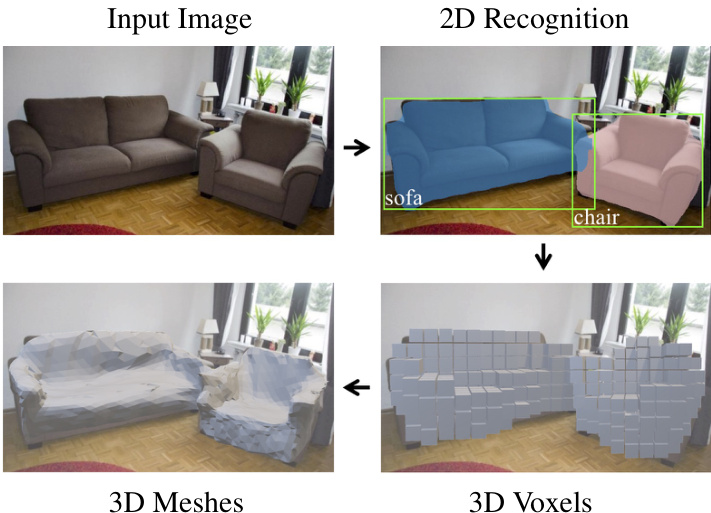
Figure 1. Mesh R-CNN takes an input image, predicts object instances in that image and infers their 3D shape. To capture diversity in geometries and topologies, it first predicts coarse voxels which are refined for accurate mesh predictions.
图 1: Mesh R-CNN 接收输入图像,预测其中的物体实例并推断其三维形状。为捕捉几何和拓扑的多样性,该方法首先生成粗略体素,再通过细化得到精确的网格预测。
We believe that the time is ripe for these hitherto distinct research directions to be combined. We should strive to build systems that (like current methods for 2D perception) can operate on un constrained real-world images with many objects, occlusion, and diverse lighting conditions but that (like current methods for 3D shape prediction) do not ignore the rich 3D structure of the world.
我们认为,将这些迄今为止独立的研究方向相结合的时机已经成熟。我们应当努力构建这样的系统:它们既能像当前二维感知方法那样处理包含多物体、遮挡和多样光照条件的无约束真实图像,又能像现有三维形状预测技术那样不忽视世界丰富的三维结构。
In this paper we take an initial step toward this goal. We draw on state-of-the-art methods for 2D perception and 3D shape prediction to build a system which inputs a real-world RGB image, detects the objects in the image, and outputs a category label, segmentation mask, and a 3D triangle mesh giving the full 3D shape of each detected object.
本文中我们朝着这一目标迈出了第一步。我们借鉴了最先进的2D感知与3D形状预测方法,构建了一个系统:输入真实世界的RGB图像后,该系统能检测图像中的物体,并输出类别标签、分割掩码以及表示每个检测物体完整3D形状的三角网格。
Our method, called Mesh R-CNN, builds on the state-ofthe-art Mask R-CNN [18] system for 2D recognition, augmenting it with a mesh prediction branch that outputs highresolution triangle meshes.
我们的方法名为Mesh R-CNN,它基于最先进的2D识别系统Mask R-CNN [18],并通过一个输出高分辨率三角网格的网格预测分支对其进行了增强。
Our predicted meshes must be able to capture the 3D structure of diverse, real-world objects. Predicted meshes should therefore dynamically vary their complexity, topology, and geometry in response to varying visual stimuli. However, prior work on mesh prediction with deep networks [23, 57, 69] has been constrained to deform from fixed mesh templates, limiting them to fixed mesh topologies. As shown in Figure 1, we overcome this limitation by utilizing multiple 3D shape representations: we first predict coarse voxelized object representations, which are converted to meshes and refined to give highly accurate mesh predictions. As shown in Figure 2, this hybrid approach allows Mesh R-CNN to output meshes of arbitrary topology while also capturing fine object structures.
我们预测的网格必须能够捕捉多样化现实物体的3D结构。因此,预测网格应根据不同视觉刺激动态调整其复杂度、拓扑结构和几何形状。然而,先前基于深度网络的网格预测研究 [23, 57, 69] 仅限于从固定网格模板进行形变,导致其拓扑结构无法改变。如图 1 所示,我们通过融合多种3D形状表示克服了这一限制:首先生成粗糙的体素化物体表示,再转换为网格并通过细化得到高精度预测结果。如图 2 所示,这种混合方法使Mesh R-CNN既能输出任意拓扑结构的网格,又能捕捉精细的物体结构。
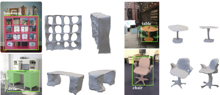
Figure 2. Example predictions from Mesh R-CNN on Pix3D. Using initial voxel predictions allows our outputs to vary in topology; converting these predictions to meshes and refining them allows us to capture fine structures like tabletops and chair legs.
图 2: Mesh R-CNN 在 Pix3D 数据集上的预测示例。通过初始体素(voxel)预测使输出具备可变拓扑结构;将这些预测转换为网格(mesh)并进行优化后,我们能捕捉到桌面和椅腿等精细结构。
We benchmark our approach on two datasets. First, we evaluate our mesh prediction branch on ShapeNet [4], where our hybrid approach of voxel prediction and mesh refinement outperforms prior work by a large margin. Second, we deploy our full Mesh R-CNN system on the recent Pix3D dataset [60] which aligns 395 models of IKEA furniture to real-world images featuring diverse scenes, clutter, and occlusion. To date Pix3D has primarily been used to evalute shape predictions for models trained on ShapeNet, using perfectly cropped, unoccluded image segments [41, 60, 73], or synthetic rendered images of Pix3D models [76]. In contrast, using Mesh R-CNN we are the first to train a system on Pix3D which can jointly detect objects of all categories and estimate their full 3D shape.
我们在两个数据集上对我们的方法进行了基准测试。首先,我们在ShapeNet [4]上评估了网格预测分支,其中我们的体素预测和网格细化混合方法大幅超越了先前的工作。其次,我们在最新的Pix3D数据集 [60]上部署了完整的Mesh R-CNN系统,该数据集将395个IKEA家具模型与包含多样化场景、杂乱和遮挡的真实世界图像对齐。迄今为止,Pix3D主要用于评估在ShapeNet上训练的模型形状预测,使用的是完美裁剪、无遮挡的图像片段 [41, 60, 73]或Pix3D模型的合成渲染图像 [76]。相比之下,使用Mesh R-CNN,我们是第一个在Pix3D上训练系统的团队,该系统可以联合检测所有类别的物体并估计它们的完整3D形状。
2. Related Work
2. 相关工作
Our system inputs a single RGB image and outputs a set of detected object instances, with a triangle mesh for each object. Our work is most directly related to recent advances in 2D object recognition and 3D shape prediction. We also draw more broadly from work on other 3D perception tasks. 2D Object Recognition Methods for 2D object recognition vary both in the type of information predicted per object, and in the overall system architecture. Object detectors output per-object bounding boxes and category labels [12, 13, 36, 38, 46, 47]; Mask R-CNN [18] additionally outputs instance segmentation masks. Our method extends this line of work to output a full 3D mesh per object.
我们的系统输入一张RGB图像,输出一组检测到的物体实例,并为每个物体生成三角网格。我们的工作最直接关联于二维物体识别和三维形状预测领域的最新进展,同时也广泛借鉴了其他三维感知任务的研究成果。
二维物体识别方法在预测每个物体的信息类型和整体系统架构上各有不同。物体检测器输出每个物体的边界框和类别标签 [12, 13, 36, 38, 46, 47];而Mask R-CNN [18] 还会输出实例分割掩码。我们的方法将这一研究方向延伸至为每个物体输出完整的三维网格。
Single-View Shape Prediction Recent approaches use a variety of shape representations for single-image 3D reconstruction. Some methods predict the orientation [10, 20] or
单视角形状预测
近期方法采用多种形状表示进行单图像3D重建。部分方法预测物体朝向[10, 20]或
3D pose [31, 44, 66] of known shapes. Other approaches predict novel 3D shapes as sets of 3D points [8, 34], patches [15, 70], or geometric primitives [9, 64, 67]; others use deep networks to model signed distance functions [42]. These methods can flexibly represent complex shapes, but rely on post-processing to extract watertight mesh outputs.
已知形状的3D位姿 [31, 44, 66]。其他方法将新颖的3D形状预测为3D点集 [8, 34]、面片 [15, 70] 或几何基元 [9, 64, 67];另一些方法使用深度网络建模有符号距离函数 [42]。这些方法能灵活表示复杂形状,但依赖后处理来提取水密网格输出。
Some methods predict regular voxel grids [5, 71, 72]; while intuitive, scaling to high-resolution outputs requires complex octree [50, 62] or nested shape architectures [49].
一些方法预测规则的体素网格 [5, 71, 72];虽然直观,但扩展到高分辨率输出需要复杂的八叉树 [50, 62] 或嵌套形状架构 [49]。
Others directly output triangle meshes, but are constrained to deform from fixed [56, 57, 69] or retrieved mesh templates [51], limiting the topologies they can represent.
其他方法直接输出三角网格,但受限于从固定 [56, 57, 69] 或检索到的网格模板 [51] 进行变形,限制了它们所能表示的拓扑结构。
Our approach uses a hybrid of voxel prediction and mesh deformation, enabling high-resolution output shapes that can flexibly represent arbitrary topologies.
我们的方法结合了体素预测 (voxel prediction) 和网格变形 (mesh deformation) ,能够生成高分辨率的输出形状,灵活表示任意拓扑结构。
Some methods reconstruct 3D shapes without 3D annotations [23, 25, 48, 68, 75]. This is an important direction, but at present we consider only the fully supervised case due to the success of strong supervision for 2D perception.
一些方法无需3D标注即可重建3D形状[23, 25, 48, 68, 75]。这是一个重要方向,但由于强监督在2D感知中的成功,目前我们仅考虑全监督场景。
Multi-View Shape Prediction There is a broad line of work on multi-view reconstruction of objects and scenes, from classical binocular stereo [17, 53] to using shape priors [1, 2, 6, 21] and modern learning techniques [24, 26, 54]. In this work, we focus on single-image shape reconstruction.
多视角形状预测
关于物体和场景的多视角重建已有大量研究,从经典的双目立体视觉 [17, 53] 到利用形状先验 [1, 2, 6, 21] 以及现代学习技术 [24, 26, 54]。本文主要关注单图像形状重建。
3D Inputs Our method inputs 2D images and predicts semantic labels and 3D shapes. Due to the increasing availabilty of depth sensors, there has been growing interest in methods predicting semantic labels from 3D inputs such as RGB-D images [16, 58] and pointclouds [14, 32, 45, 59, 63]. We anticipate that incorporating 3D inputs into our method could improve the fidelity of our shape predictions.
3D输入
我们的方法输入2D图像并预测语义标签和3D形状。由于深度传感器的日益普及,人们对从RGB-D图像[16, 58]和点云[14, 32, 45, 59, 63]等3D输入预测语义标签的方法越来越感兴趣。我们预计将3D输入纳入我们的方法可以提高形状预测的保真度。
Datasets Advances in 2D perception have been driven by large-scale annotated datasets such as ImageNet [52] and COCO [37]. Datasets for 3D shape prediction have lagged their 2D counterparts due to the difficulty of collecting 3D annotations. ShapeNet [4] is a large-scale dataset of CAD models which are rendered to give synthetic images. The IKEA dataset [33] aligns CAD models of IKEA objects to real-world images; Pix3D [60] extends this idea to a larger set of images and models. Pascal3D [74] aligns CAD models to real-world images, but it is unsuitable for shape recon- struction since its train and test sets share the same small set of models. KITTI [11] annotates outdoor street scenes with 3D bounding boxes, but does not provide shape annotations.
数据集
2D感知的进步得益于ImageNet [52]和COCO [37]等大规模标注数据集的推动。由于3D标注数据收集困难,3D形状预测数据集的发展一直落后于2D领域。ShapeNet [4]是一个包含CAD模型的大规模数据集,这些模型经过渲染生成合成图像。IKEA数据集 [33]将宜家物品的CAD模型与现实图像对齐;Pix3D [60]将这一理念扩展到更多图像和模型。Pascal3D [74]虽然也将CAD模型与现实图像对齐,但由于其训练集和测试集共享同一小批模型,不适合用于形状重建。KITTI [11]为户外街景标注了3D边界框,但未提供形状标注数据。
3. Method
3. 方法
Our goal is to design a system that inputs a single image, detects all objects, and outputs a category label, bounding box, segmentation mask and 3D triangle mesh for each detected object. Our system must be able to handle cluttered real-world images, and must be trainable end-to-end. Our output meshes should not be constrained to a fixed topology in order to accommodate a wide variety of complex real-world objects. We accomplish these goals by marrying state-of-the-art 2D perception with 3D shape prediction.
我们的目标是设计一个系统,能够输入单张图像、检测所有物体,并为每个检测到的物体输出类别标签、边界框、分割掩码和3D三角网格。该系统必须能处理杂乱的真实世界图像,且支持端到端训练。为确保适应各种复杂现实物体,输出网格不应受固定拓扑结构限制。我们通过融合最先进的2D感知与3D形状预测技术来实现这些目标。
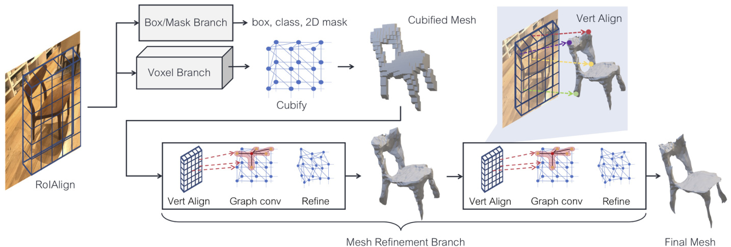
Figure 3. System overview of Mesh R-CNN. We augment Mask R-CNN with 3D shape inference. The voxel branch predicts a coarse shape for each detected object which is further deformed with a sequence of refinement stages in the mesh refinement branch.
图 3: Mesh R-CNN 系统概览。我们在 Mask R-CNN 基础上增加了 3D 形状推断功能。体素分支为每个检测到的物体预测粗略形状,随后通过网格优化分支中的多级细化阶段进行进一步变形。
Specifically, we build on Mask R-CNN [18], a state-ofthe-art 2D perception system. Mask R-CNN is an end-toend region-based object detector. It inputs a single RGB image and outputs a bounding box, category label, and segmentation mask for each detected object. The image is first passed through a backbone network (e.g. ResNet-50- FPN [35]); next a region proposal network (RPN) [47] gives object proposals which are processed with object classification and mask prediction branches.
具体来说,我们基于当前最先进的2D感知系统Mask R-CNN [18]进行构建。Mask R-CNN是一种端到端的基于区域的目标检测器。它输入单个RGB图像,并为每个检测到的目标输出边界框、类别标签和分割掩码。图像首先通过主干网络(例如ResNet-50-FPN [35])处理;接着区域提议网络(RPN) [47]生成目标提议,这些提议通过目标分类和掩码预测分支进行处理。
Part of Mask R-CNN’s success is due to RoIAlign which extracts region features from image features while maintaining alignment between the input image and features used in the final prediction branches. We aim to maintain similar feature alignment when predicting 3D shapes.
Mask R-CNN 的成功部分归功于 RoIAlign (Region of Interest Align),它从图像特征中提取区域特征,同时保持输入图像与最终预测分支所用特征之间的对齐。我们的目标是在预测 3D 形状时保持类似的特征对齐。
We infer 3D shapes with a novel mesh predictor, comprising a voxel branch and a mesh refinement branch. The voxel branch first estimates a coarse 3D vox eliza tion of an object, which is converted to an initial triangle mesh. The mesh refinement branch then adjusts the vertex positions of this initial mesh using a sequence of graph convolution layers operating over the edges of the mesh.
我们采用一种新颖的网格预测器来推断3D形状,该预测器包含一个体素分支和一个网格优化分支。体素分支首先估计物体的粗略3D体素化表示,随后将其转换为初始三角形网格。网格优化分支则通过一系列作用于网格边缘的图卷积层,调整该初始网格的顶点位置。
The voxel branch and mesh refinement branch are homologous to the existing box and mask branches of Mask RCNN. All take as input image-aligned features corresponding to RPN proposals. The voxel and mesh losses, described in detail below, are added to the box and mask losses and the whole system is trained end-to-end. The output is a set of boxes along with their predicted object scores, masks and 3D shapes. We call our system Mesh R-CNN, which is illustrated in Figure 3.
体素分支和网格优化分支与现有Mask RCNN的检测框分支、掩码分支同源。它们都以区域提议网络(RPN)生成的图像对齐特征作为输入。下文将详述的体素损失和网格损失,会与检测框损失、掩码损失共同构成损失函数,整个系统采用端到端训练。最终输出为带预测物体分数的检测框集合,及其对应的掩码和三维形状。我们将该系统命名为Mesh R-CNN,其架构如图3所示。
We now describe our mesh predictor, consisting of the voxel branch and mesh refinement branch, along with its associated losses in detail.
我们现在详细描述由体素分支和网格优化分支组成的网格预测器及其相关损失函数。
3.1. Mesh Predictor
3.1. Mesh Predictor
At the core of our system is a mesh predictor which receives convolutional features aligned to an object’s bounding box and predicts a triangle mesh giving the object’s full 3D shape. Like Mask R-CNN, we maintain correspondence between the input image and features used at all stages of processing via region- and vertex-specific alignment operators (RoIAlign and VertAlign). Our goal is to capture instance-specific 3D shapes of all objects in an image. Thus, each predicted mesh must have instance-specific topology (genus, number of vertices, faces, connected components) and geometry (vertex positions).
我们系统的核心是一个网格预测器,它接收与物体边界框对齐的卷积特征,并预测给出物体完整3D形状的三角网格。与Mask R-CNN类似,我们通过区域和顶点特定的对齐操作(RoIAlign和VertAlign)保持输入图像与处理各阶段所用特征之间的对应关系。我们的目标是捕捉图像中所有物体的实例特定3D形状。因此,每个预测网格必须具有实例特定的拓扑结构(亏格、顶点数量、面数、连通分量)和几何结构(顶点位置)。
We predict varying mesh topologies by deploying a sequence of shape inference operations. First, the voxel branch makes bottom-up voxelized predictions of each object’s shape, similar to Mask R-CNN’s mask branch. These predictions are converted into meshes and adjusted by the mesh refinement head, giving our final predicted meshes.
我们通过部署一系列形状推断操作来预测不同的网格拓扑结构。首先,体素分支自底向上对每个物体的形状进行体素化预测,类似于Mask R-CNN的掩码分支。这些预测被转换为网格,并通过网格优化头进行调整,最终得到我们预测的网格。
The output of the mesh predictor is a triangle mesh $T=$ $(V,F)$ for each object. $V={v_{i}\in\mathbb{R}^{3}}$ is the set of vertex positions and $F\subseteq V\times V\times V$ is a set of triangular faces.
网格预测器的输出是每个对象的三角形网格 $T=$ $(V,F)$。$V={v_{i}\in\mathbb{R}^{3}}$ 是顶点位置集合,$F\subseteq V\times V\times V$ 是一组三角形面。
3.1.1 Voxel Branch
3.1.1 体素分支
The voxel branch predicts a grid of voxel occupancy probabilities giving the course 3D shape of each detected object. It can be seen as a 3D analogue of Mask R-CNN’s mask prediction branch: rather than predicting a $M\times M$ grid giving the object’s shape in the image plane, we instead predict a $G\times G\times G$ grid giving the object’s full 3D shape.
体素分支预测一个体素占据概率的网格,给出每个检测物体的粗略3D形状。可以将其视为Mask R-CNN掩码预测分支的3D对应:不同于预测图像平面中物体形状的$M\times M$网格,我们改为预测给出物体完整3D形状的$G\times G\times G$网格。
Like Mask R-CNN, we maintain correspondence between input features and predicted voxels by applying a small fully-convolutional network [39] to the input feature map resulting from RoIAlign. This network produces a feature map with $G$ channels giving a column of voxel occupancy scores for each position in the input.
与 Mask R-CNN 类似,我们通过在 RoIAlign 生成的输入特征图上应用小型全卷积网络 [39] 来保持输入特征与预测体素之间的对应关系。该网络会生成具有 $G$ 个通道的特征图,为输入中的每个位置提供一列体素占用分数。
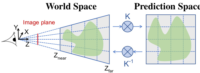
Figure 4. Predicting voxel occ up an cie s aligned to the image plane requires an irregularly-shaped voxel grid. We achieve this effect by making voxel predictions in a space that is transformed by the camera’s (known) intrinsic matrix $K$ . Applying $K^{-1}$ transforms our predictions back to world space. This results in frustumshaped voxels in world space.
图 4: 预测与图像平面对齐的体素占用需要不规则形状的体素网格。我们通过在经过相机(已知)内参矩阵 $K$ 变换的空间中进行体素预测来实现这一效果。应用 $K^{-1}$ 将预测结果转换回世界坐标系,从而在世界空间中形成锥台形状的体素。
Maintaining pixelwise correspondence between the image and our predictions is complex in 3D since objects become smaller as they recede from the camera. As shown in Figure 4, we account for this by using the camera’s (known) intrinsic matrix to predict frustum-shaped voxels.
在3D场景中保持图像与预测结果之间的像素级对应关系十分复杂,因为物体会随着远离相机而逐渐变小。如图4所示,我们通过利用相机(已知)内参矩阵预测截头体形状的体素来解决这一问题。
Cubify: Voxel to Mesh The voxel branch produces a 3D grid of occupancy probabilities giving the coarse shape of an object. In order to predict more fine-grained 3D shapes, we wish to convert these voxel predictions into a triangle mesh which can be passed to the mesh refinement branch.
Cubify: 体素转网格
体素分支生成一个3D占据概率网格,提供物体的粗略形状。为了预测更精细的3D形状,我们希望将这些体素预测转换为三角形网格,以便传递给网格优化分支。
We bridge this gap with an operation called cubify. It inputs voxel occupancy probabilities and a threshold for binarizing voxel occupancy. Each occupied voxel is replaced with a cuboid triangle mesh with 8 vertices, 18 edges, and 12 faces. Shared vertices and edges between adjacent occupied voxels are merged, and shared interior faces are eliminated. This results in a watertight mesh whose topology depends on the voxel predictions.
我们通过一种称为立方化(cubify)的操作来弥合这一差距。该操作输入体素占据概率和用于二值化体素占据的阈值。每个被占据的体素会被替换为一个包含8个顶点、18条边和12个面的长方体三角网格。相邻被占据体素之间的共享顶点和边会被合并,共享的内部面会被消除。这样会产生一个拓扑结构取决于体素预测结果的防水网格。
Cubify must be efficient and batched. This is not trivial and we provide technical implementation details of how we achieve this in Appendix A. Alternatively marching cubes [40] could extract an isosurface from the voxel grid, but is significantly more complex.
Cubify 必须高效且批量化处理。这并非易事,我们在附录 A 中提供了实现这一目标的技术细节。另一种方案是使用移动立方体算法 (marching cubes) [40] 从体素网格中提取等值面,但实现复杂度显著更高。
Voxel Loss The voxel branch is trained to minimize the binary cross-entropy between predicted voxel occupancy probabilities and true voxel occ up an cie s.
体素损失 (Voxel Loss)
体素分支的训练目标是最小化预测体素占用概率与真实体素占用之间的二元交叉熵。
3.1.2 Mesh Refinement Branch
3.1.2 网格细化分支
The cubified mesh from the voxel branch only provides a coarse 3D shape, and it cannot accurately model fine structures like chair legs. The mesh refinement branch processes this initial cubified mesh, refining its vertex positions with a sequence of refinement stages. Similar to [69], each refinement stage consists of three operations: vertex alignment, which extracts image features for vertices; graph convolution, which propagates information along mesh edges; and vertex refinement, which updates vertex positions. Each layer of the network maintains a 3D position $v_{i}$ and a feature vector $f_{i}$ for each mesh vertex.
体素分支生成的立方化网格仅提供粗糙的3D形状,无法准确建模椅子腿等精细结构。网格细化分支通过多级细化阶段处理初始立方化网格:每个阶段包含三项操作——顶点对齐(提取顶点图像特征)、图卷积(沿网格边传播信息)和顶点细化(更新顶点位置)。如[69]所述,网络每层为网格顶点维护三维位置$v_{i}$和特征向量$f_{i}$。
Vertex Alignment yields an image-aligned feature vector for each mesh vertex1. We use the camera’s intrinsic matrix to project each vertex onto the image plane. Given a feature map, we compute a bilinearly interpolated image feature at each projected vertex position [22].
顶点对齐 (Vertex Alignment) 为每个网格顶点生成图像对齐的特征向量。我们使用相机内参矩阵将每个顶点投影到图像平面上。给定特征图时,我们会在每个投影顶点位置计算双线性插值图像特征 [22]。
In the first stage of the mesh refinement branch, VertAlign outputs an initial feature vector for each vertex. In subsequent stages, the VertAlign output is concatenated with the vertex feature from the previous stage.
在网格细化分支的第一阶段,VertAlign为每个顶点输出初始特征向量。在后续阶段,VertAlign的输出会与前一阶段的顶点特征进行拼接。
Graph Convolution [29] propagates information along mesh edges. Given input vertex features ${f_{i}}$ it computes updated features $\begin{array}{r}{f_{i}^{\prime}=\operatorname{ReLU}\left(W_{0}f_{i}+\sum_{j\in\mathcal{N}(i)}W_{1}f_{j}\right)}\end{array}$ where $\mathcal{N}(i)$ gives the $i$ -th vertex’s neighb ors in the mesh, and $W_{0}$ and $W_{1}$ are learned weight matrices. Each stage of the mesh refinement branch uses several graph convolution layers to aggregate information over local mesh regions.
图卷积 [29] 沿网格边传播信息。给定输入顶点特征 ${f_{i}}$,它计算更新后的特征 $\begin{array}{r}{f_{i}^{\prime}=\operatorname{ReLU}\left(W_{0}f_{i}+\sum_{j\in\mathcal{N}(i)}W_{1}f_{j}\right)}\end{array}$,其中 $\mathcal{N}(i)$ 表示网格中第 $i$ 个顶点的邻接顶点,$W_{0}$ 和 $W_{1}$ 为可学习的权重矩阵。网格细化分支的每个阶段都使用多个图卷积层来聚合局部网格区域的信息。
Vertex Refinement computes updated vertex positions $v_{i}^{\prime}=v_{i}+\operatorname{tanh}(W_{v e r t}\left[f_{i};v_{i}\right])$ where $W_{v e r t}$ is a learned weight matrix. This updates the mesh geometry, keeping its topology fixed. Each stage of the mesh refinement branch terminates with vertex refinement, producing an intermediate mesh output which is further refined by the next stage.
顶点优化 (Vertex Refinement) 计算更新后的顶点位置 $v_{i}^{\prime}=v_{i}+\operatorname{tanh}(W_{v e r t}\left[f_{i};v_{i}\right])$ ,其中 $W_{v e r t}$ 是学习得到的权重矩阵。该操作在保持网格拓扑不变的情况下更新几何形状。网格优化分支的每个阶段都以顶点优化作为终止步骤,生成中间网格输出供下一阶段继续优化。
Mesh Losses Defining losses that operate natively on triangle meshes is challenging, so we instead use loss functions defined over a finite set of points. We represent a mesh with a pointcloud by densely sampling its surface. Consequently, a pointcloud loss approximates a loss over shapes.
网格损失
定义直接在三角形网格上操作的损失具有挑战性,因此我们改用基于有限点集定义的损失函数。我们通过密集采样网格表面,用点云表示网格。因此,点云损失可近似视为形状损失。
Similar to [57], we use a differentiable mesh sampling operation to sample points (and their normal vectors) uniformly from the surface of a mesh. To this end, we implement an efficient batched sampler; see Appendix B for details. We use this operation to sample a pointcloud $P^{g t}$ from the ground-truth mesh, and a pointcloud $P^{i}$ from each intermediate mesh prediction from our model.
与[57]类似,我们采用可微分网格采样操作从网格表面均匀采样点(及其法向量)。为此,我们实现了一个高效的批量采样器(详见附录B)。通过该操作,我们从真实值网格中采样点云$P^{gt}$,并从模型的每个中间网格预测中采样点云$P^{i}$。
Given two point clouds $P,Q$ with normal vectors, let $\Lambda_{P,Q}={(p,\mathrm{arg}\operatorname*{min}{q}|p-q|):p\in P}$ be the set of pairs $(p,q)$ such that $q$ is the nearest neighbor of $p$ in $Q$ , and let $u_{p}$ be the unit normal to point $p$ . The chamfer distance between point clouds $P$ and $Q$ is given by
给定两个带法向量的点云 $P,Q$,设 $\Lambda_{P,Q}={(p,\mathrm{arg}\operatorname*{min}{q}|p-q|):p\in P}$ 为所有点对 $(p,q)$ 的集合,其中 $q$ 是 $Q$ 中离 $p$ 最近的点,$u_{p}$ 表示点 $p$ 的单位法向量。点云 $P$ 与 $Q$ 之间的倒角距离 (chamfer distance) 由以下公式给出:
$$
\mathcal{L}{\mathrm{cham}}(P,Q)=|P|^{-1}\sum_{(p,q)\in\Lambda_{P,Q}}|p-q|^{2}+|Q|^{-1}\sum_{(q,p)\in\Lambda_{Q,P}}|q-p|^{2}
$$
$$
\mathcal{L}{\mathrm{cham}}(P,Q)=|P|^{-1}\sum_{(p,q)\in\Lambda_{P,Q}}|p-q|^{2}+|Q|^{-1}\sum_{(q,p)\in\Lambda_{Q,P}}|q-p|^{2}
$$
and the (absolute) normal distance is given by
且(绝对)法向距离由下式给出
$$
\mathcal{L}{\mathrm{norm}}(P,Q)=-|P|^{-1}\sum_{(p,q)\in\Lambda_{P,Q}}|u_{p}\cdot u_{q}|-|Q|^{-1}\sum_{(q,p)\in\Lambda_{Q,P}}|u_{q}\cdot u_{p}|.
$$
$$
\mathcal{L}{\mathrm{norm}}(P,Q)=-|P|^{-1}\sum_{(p,q)\in\Lambda_{P,Q}}|u_{p}\cdot u_{q}|-|Q|^{-1}\sum_{(q,p)\in\Lambda_{Q,P}}|u_{q}\cdot u_{p}|.
$$
The chamfer and normal distances penalize mismatched positions and normals between two point clouds, but minimizing these distances alone results in degenerate meshes (see Figure 5). High-quality mesh predictions require additional shape regularize rs: To this end we use an edge loss $\begin{array}{r}{\mathcal{L}{\mathrm{edge}}(V,\bar{E})=\frac{1}{\vert E\vert}\sum_{(v,v^{\prime})\in E}\Vert v-v^{\prime}\Vert^{2}}\end{array}$ where $E\subseteq V\times V$ are the edges of the predicted mesh. Alternatively, a Laplacian loss [7] also imposes smoothness constraints.
倒角距离和法线距离惩罚了两个点云之间不匹配的位置和法线,但仅最小化这些距离会导致网格退化 (参见图 5)。高质量的网格预测需要额外的形状正则化器:为此我们使用边缘损失 $\begin{array}{r}{\mathcal{L}{\mathrm{edge}}(V,\bar{E})=\frac{1}{\vert E\vert}\sum_{(v,v^{\prime})\in E}\Vert v-v^{\prime}\Vert^{2}}\end{array}$ 其中 $E\subseteq V\times V$ 是预测网格的边。另外,拉普拉斯损失 [7] 也施加了平滑约束。
The mesh loss of the $i$ -th stage is a weighted sum of $\mathcal{L}{\mathrm{cham}}(P^{i},P^{g t})$ , $\mathcal{L}{\mathrm{{norm}}}(P^{i},P^{g t})$ and $\mathcal{L}_{\mathrm{edge}}(V^{i},E^{i})$ . The mesh refinement branch is trained to minimize the mean of these losses across all refinement stages.
第 $i$ 阶段的网格损失是 $\mathcal{L}{\mathrm{cham}}(P^{i},P^{g t})$ 、 $\mathcal{L}{\mathrm{{norm}}}(P^{i},P^{g t})$ 和 $\mathcal{L}_{\mathrm{edge}}(V^{i},E^{i})$ 的加权和。网格优化分支的训练目标是最小化所有优化阶段这些损失的平均值。
4. Experiments
4. 实验
We benchmark our mesh predictor on ShapeNet [4], where we compare with state-of-the-art approaches. We then evaluate our full Mesh R-CNN for the task of 3D shape prediction in the wild on the challenging Pix3D dataset [60].
我们在ShapeNet [4]上对网格预测器进行了基准测试,并与最先进的方法进行了比较。随后,我们在具有挑战性的Pix3D数据集 [60] 上评估了完整Mesh R-CNN在真实场景3D形状预测任务中的表现。
4.1. ShapeNet
4.1. ShapeNet
ShapeNet [4] provides a collection of 3D shapes, represented as textured CAD models organized into semantic categories following WordNet [43], and has been widely used as a benchmark for 3D shape prediction. We use the subset of Shape Net Core.v1 and rendered images from [5]. Each mesh is rendered from up to 24 random viewpoints, giving RGB images of size $137\times137$ . We use the train / test splits provided by [69], which allocate 35,011 models (840,189 images) to train and 8,757 models (210,051 images) to test; models used in train and test are disjoint. We reserve $5%$ of the training models as a validation set.
ShapeNet [4] 提供了一个3D形状集合,这些形状以带纹理的CAD模型形式呈现,并按照WordNet [43]的语义类别进行组织,已被广泛用作3D形状预测的基准。我们使用ShapeNet Core.v1的子集及来自[5]的渲染图像。每个网格从最多24个随机视角渲染,生成尺寸为$137\times137$的RGB图像。我们采用[69]提供的训练/测试划分方案:35,011个模型(840,189张图像)用于训练,8,757个模型(210,051张图像)用于测试,且训练集与测试集的模型互不重叠。我们预留$5%$的训练模型作为验证集。
The task on this dataset is to input a single RGB image of a rendered ShapeNet model on a blank background, and output a 3D mesh for the object in the camera coordinate system. During training the system is supervised with pairs of images and meshes.
该数据集的任务是输入一张在空白背景上渲染的ShapeNet模型的RGB图像,并输出相机坐标系中物体的3D网格。训练期间系统通过图像和网格配对数据进行监督学习。
Evaluation We adopt evaluation metrics used in recent work [56, 57, 69]. We sample 10k points uniformly at random from the surface of predicted and ground-truth meshes, and use them to compute Chamfer distance (Equation 1), Normal consistency, (one minus Equation 2), and $\mathrm{F}1^{\tau}$ at various distance thresholds $\tau$ , which is the harmonic mean of the precision at $\tau$ (fraction of predicted points within $\tau$ of a ground-truth point) and the recall at $\tau$ (fraction of groundtruth points within $\tau$ of a predicted point). Lower is better for Chamfer distance; higher is better for all other metrics.
评估
我们采用近期研究[56, 57, 69]中使用的评估指标。从预测和真实网格表面均匀随机采样10k个点,用于计算倒角距离(Chamfer distance)(公式1)、法向一致性(Normal consistency)(1减去公式2),以及不同距离阈值$\tau$下的$\mathrm{F}1^{\tau}$(即$\tau$处精度(预测点中距离真实点小于$\tau$的比例)与$\tau$处召回率(真实点中距离预测点小于$\tau$的比例)的调和平均数)。倒角距离越小越好,其他指标均为越大越好。
With the exception of normal consistency, these metrics depend on the absolute scale of the meshes. In Table 1 we follow [69] and rescale by a factor of 0.57; for all other results we follow [8] and rescale so the longest edge of the ground-truth mesh’s bounding box has length 10.
除了常规一致性外,这些指标还取决于网格的绝对比例。在表1中,我们遵循[69]的方法,按0.57的系数进行缩放;对于所有其他结果,我们遵循[8]的方法进行缩放,使真实网格包围盒的最长边长度为10。
Implementation Details Our backbone feature extractor is ResNet-50 pretrained on ImageNet. Since images depict a single object, the voxel branch receives the entire $\mathtt{C O n v5}_{-3}$ feature map, bilinearly resized to $24\times24$ , and predicts a $48\times48\times48$ voxel grid. The VertAlign operator concatenates features from conv2 3, conv3 4, conv4 6, and conv5 3 before projecting to a vector of dimension
实现细节
我们的主干特征提取器是在ImageNet上预训练的ResNet-50。由于图像描绘的是单个对象,体素分支接收整个$\mathtt{C O n v5}_{-3}$特征图,并通过双线性调整大小至$24\times24$,然后预测一个$48\times48\times48$的体素网格。VertAlign操作符在投影到维度向量之前,将来自conv2_3、conv3_4、conv4_6和conv5_3的特征进行拼接。
| Chamfer(↓) | F1(↑) F12 (↑) | |
|---|---|---|
| N3MR [25] | 2.629 | 33.80 47.72 |
| 3D-R2N2 [5] | 1.445 | 39.01 54.62 |
| PSG [8] | 0.593 | 48.58 69.78 |
| Pixel2Mesh [69] | 0.591 | 59.72 74.19 |
| MVD [56] | 66.39 | |
| GEOMetrics [57] | 67.37 | |
| Pixel2Mesh [69] | 0.463 | 67.89 79.88 |
| Ours (Best) | 0.306 | 74.84 85.75 |
| Ours (Pretty) | 0.391 69.83 | 81.76 |
Table 1. Single-image shape reconstruction results on ShapeNet, using the evaluation protocol from [69]. For [69], † are results reported in their paper and ‡ is the model released by the authors.
表 1: ShapeNet 单图像形状重建结果,采用 [69] 的评估协议。[69] 中 † 表示论文报告结果,‡ 表示作者发布的模型。
- The mesh refinement branch has three stages, each with six graph convolution layers (of dimension 128) organized into three residual blocks. We train for 25 epochs using Adam [27] with learning rate $10^{-4}$ and 32 images per batch on 8 Tesla V100 GPUs. We set the cubify threshold to 0.2 and weight the losses with $\lambda_{\mathrm{voxel}}=1$ , $\lambda_{\mathrm{cham}}=1$ , $\lambda_{\mathrm{norm}}=0$ , and $\lambda_{\mathrm{edge}}=0.2$ .
- 网格细化分支包含三个阶段,每个阶段由六个维度为128的图卷积层组成,分为三个残差块。训练采用Adam优化器[27],学习率为$10^{-4}$,在8块Tesla V100 GPU上以每批次32张图像进行25轮训练。设置立方化阈值为0.2,损失权重分别为$\lambda_{\mathrm{voxel}}=1$、$\lambda_{\mathrm{cham}}=1$、$\lambda_{\mathrm{norm}}=0$和$\lambda_{\mathrm{edge}}=0.2$。
Baselines We compare with previously published methods for single-image shape prediction. N3MR [25] is a weakly supervised approach that fits a mesh via a differentiable renderer without 3D supervision. 3D-R2N2 [5] and MVD [56] output voxel predictions. PSG [8] predicts point-clouds. Appendix D additionally compares with OccNet [42].
基线方法
我们与已发表的单图像形状预测方法进行比较。N3MR [25] 是一种弱监督方法,通过可微分渲染器拟合网格,无需3D监督。3D-R2N2 [5] 和 MVD [56] 输出体素预测结果。PSG [8] 预测点云。附录 D 还额外对比了 OccNet [42]。
Pixel2Mesh [69] predicts meshes by deforming and subdividing an initial ellipsoid. GEOMetrics [57] extends [69] with adaptive face subdivision. Both are trained to minimize Chamfer distances; however [69] computes it using predicted mesh vertices, while [57] uses points sampled uniformly from predicted meshes. We adopt the latter as it better matches test-time evaluation. Unlike ours, these methods can only predict connected meshes of genus zero.
Pixel2Mesh [69] 通过变形和细分初始椭球体来预测网格。GEOMetrics [57] 在 [69] 的基础上扩展了自适应面细分。两者都训练以最小化 Chamfer 距离;然而 [69] 使用预测的网格顶点计算该距离,而 [57] 使用从预测网格中均匀采样的点。我们采用后者,因其更匹配测试时的评估。与我们的方法不同,这些方法只能预测零亏格的连通网格。
The training recipe and backbone architecture vary among prior work. Therefore for a fair comparison with our method we also compare against several ablated versions of our model (see Appendix C for exact details):
先前工作中的训练方案和骨干架构各不相同。因此为了与我们的方法进行公平比较,我们还对比了本模型的若干消融版本(具体细节参见附录C):
Voxel-Only: A version of our method that terminates with the cubified meshes from the voxel branch. Pixel2Mesh+: We re implement Pixel2Mesh [69]; we outperform their original model due to a deeper backbone, better training recipe, and minimizing Chamfer on sampled rather than vertex positions. Sphere-Init: Similar to $\mathrm{Pixel}2\mathbf{M}\mathrm{esh}^{+}$ , but initializes from a high-resolution sphere mesh, performing three stages of vertex refinement without subdivision. Ours (light): Uses a smaller non residual mesh refinement branch with three graph convolution layers per stage. We will adopt this lightweight design on Pix3D.
体素分支 (Voxel-Only):本方法的终止版本,直接输出体素分支生成的立方化网格。
Pixel2Mesh+:我们复现了 Pixel2Mesh [69],通过更深的骨干网络、改进的训练方案,以及在采样点而非顶点位置优化倒角距离 (Chamfer),性能超越了原模型。
球面初始化 (Sphere-Init):与 $\mathrm{Pixel}2\mathbf{M}\mathrm{esh}^{+}$ 类似,但从高分辨率球面网格初始化,在不细分的情况下执行三阶段顶点优化。
轻量版 (Ours (light)):采用非残差结构的轻量化网格优化分支,每阶段仅含三层图卷积。该轻量设计将应用于 Pix3D 数据集。
Voxel-Only is essentially a version of our method that omits the mesh refinement branch, while Pixel2Mesh+ and Sphere-Init omit the voxel prediction branch.
Voxel-Only本质上是我们方法的变体,省略了网格优化分支,而Pixel2Mesh+和Sphere-Init则省略了体素预测分支。
Table 2. We report results both on the full ShapeNet test set (left), as well as a subset of the test set consisting of meshes with visible holes (right). We compare our full model with several ablated version: Voxel-Only omits the mesh refinement head, while Sphere-Init and $\mathrm{Pixel}2\mathrm{Mesh}^{+}$ omit the voxel head. We show results both for Best models which optimize for metrics, as well as Pretty models that strike a balance between shape metrics and mesh quality (see Figure 5); these two categories of models should not be compared. We also report the number of vertices $|V|$ and faces $|F|$ in predicted meshes (mean $\pm\mathrm{std}$ ). ‡ refers to the released model by the authors. (per-instance average)
表 2. 我们在完整 ShapeNet 测试集 (左) 和包含可见孔洞网格的子测试集 (右) 上报告结果。我们将完整模型与多个消融版本进行比较: Voxel-Only 省略了网格细化头, 而 Sphere-Init 和 $\mathrm{Pixel}2\mathrm{Mesh}^{+}$ 省略了体素头。我们展示了针对指标优化的 Best 模型结果, 以及在形状指标和网格质量之间取得平衡的 Pretty 模型结果 (见图 5); 这两类模型不可直接比较。我们还报告了预测网格中的顶点数 $|V|$ 和面数 $|F|$ (均值 $\pm\mathrm{std}$)。‡ 表示作者发布的模型。(单实例平均值)
| 完整测试集 | 孔洞测试集 | ||||||||||||||
|---|---|---|---|---|---|---|---|---|---|---|---|---|---|---|---|
| Chamfer(↓) | Normal | F10.1 | F10.3 | F10.5 | [V] | [F | Chamfer(↓) | Normal | F10.1 | F10.3 | F10.5 | [V] | |||
| Pixel2Mesh [69] | 0.205 | 0.736 | 33.7 | 80.9 | 91.7 | 2466±0 | 4928±0 | 0.272 | 0.689 | 31.5 | 75.9 | 87.9 | 2466±0 | 4928±0 | |
| Voxel-Only | 0.916 | 0.595 | 7.7 | 33.1 | 54.9 | 1987±936 | 3975±1876 | 0.760 | 0.592 | 8.2 | 35.7 | 59.5 | 2433±925 | 4877±1856 | |
| Sphere-Init | 0.132 | 0.711 | 38.3 | 86.5 | 95.1 | 2562±0 | 5120±0 | 0.138 | 0.705 | 40.0 | 85.4 | 94.3 | 2562±0 | 5120±0 | |
| Pixel2Mesh+ | 0.132 | 0.707 | 38.3 | 86.6 | 95.1 | 2562±0 | 5120±0 | 0.137 | 0.696 | 39.3 | 85.5 | 94.4 | 2562±0 | 5120±0 | |
| B Ours | Ours (light) | 0.133 | 0.725 | 39.2 | 86.8 | 95.1 | 1894±925 | 3791±1855 | 0.130 | 0.723 | 41.6 | 86.7 | 94.8 | 2273±899 | 4560±1805 |
| 0.133 | 0.729 | 38.8 | 86.6 | 95.1 | 1899±928 | 3800±1861 | 0.130 | 0.725 | 41.7 | 86.7 | 94.9 | 2291±903 | 4595±1814 | ||
| Sphere-Init | 0.175 | 0.718 | 34.5 | 82.2 | 92.9 | 2562±0 | 5120±0 | 0.186 | 0.684 | 34.4 | 80.2 | 91.7 | 2562±0 | 5120±0 | |
| Pixel2Mesh+ | 0.175 | 0.727 | 34.9 | 82.3 | 92.9 | 2562±0 | 5120±0 | 0.196 | 0.685 | 34.4 | 79.9 | 91.4 | 2562±0 | 5120±0 | |
| Pret | Ours (light) | 0.176 | 0.699 | 34.8 | 82.4 | 93.1 | 1891±924 | 3785±1853 | 0.178 | 0.688 | 36.3 | 82.0 | 92.4 | 2281±895 | 4576±1798 |
| Ours | 0.171 | 0.713 | 35.1 | 82.6 | 93.2 | 1896±928 | 3795±1861 | 0.171 | 0.700 | 37.1 | 82.4 | 92.7 | 2292±902 | 4598±1812 |
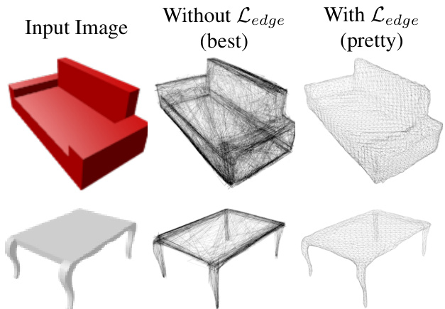
Figure 5. Training without the edge length regularize r $\mathcal{L}{e d g e}$ results in degenerate predicted meshes that have many overlapping faces. Adding $\mathcal{L}_{e d g e}$ eliminates this degeneracy but results in worse agreement with the ground-truth as measured by standard metrics such as Chamfer distance.
图 5: 未使用边长正则项 $\mathcal{L}{edge}$ 进行训练时,预测网格会出现包含大量重叠面的退化情况。加入 $\mathcal{L}_{edge}$ 后虽然消除了这种退化现象,但根据Chamfer距离等标准指标衡量,其与真实值的匹配度会下降。
Best vs Pretty As previously noted in [69] (Section 4.1), standard metrics for shape reconstruction are not wellcorrelated with mesh quality. Figure 5 shows that models trained without shape regularize rs give meshes that are preferred by metrics despite being highly degenerate, with irregularly-sized faces and many self-intersections. These degenerate meshes would be difficult to texture, and may not be useful for downstream applications.
最佳与美观
如[69](第4.1节)所述,形状重建的标准指标与网格质量相关性不高。图5显示,未经形状正则化器训练的模型生成的网格在指标上更受青睐,但这些网格存在高度退化问题,包括不规则尺寸的面和大量自相交。这些退化网格难以进行纹理处理,可能不适用于下游应用。
Due to the strong effect of shape regularize rs on both mesh quality and quantitative metrics, we suggest only quantitatively comparing methods trained with the same shape regularize rs. We thus train two versions of all our ShapeNet models: a Best version with $\lambda_{\mathrm{edge}}=0$ to serve as an upper bound on quantitative performance, and a Pretty version that strikes a balance between quantitative performance and mesh quality by setting $\lambda_{\mathrm{edge}}=0.2$ .
由于形状正则化器对网格质量和量化指标均有显著影响,我们建议仅定量比较采用相同形状正则化器训练的方法。因此,我们为所有ShapeNet模型训练了两个版本:性能上限版(Best)设置$\lambda_{\mathrm{edge}}=0$以实现量化性能最优,均衡版(Pretty)通过设定$\lambda_{\mathrm{edge}}=0.2$在量化性能与网格质量间取得平衡。
Comparison with Prior Work Table 1 compares our Pretty and Best models with prior work on shape prediction from a single image. We use the evaluation protocol from [69], using a 0.57 mesh scaling factor and threshold value $\tau=$ $10^{-4}$ on squared Euclidean distances. For Pixel2Mesh, we provide the performance reported in their paper [69] as well as the performance of their open-source pretrained model. Table 1 shows that we outperform prior work by a wide margin, validating the design of our mesh predictor.
与先前工作的比较
表 1 将我们的 Pretty 和 Best 模型与单图像形状预测的先前工作进行了比较。我们采用 [69] 中的评估协议,使用 0.57 的网格缩放因子和平方欧氏距离的阈值 $\tau=$ $10^{-4}$。对于 Pixel2Mesh,我们提供了其论文 [69] 中报告的性能以及其开源预训练模型的性能。表 1 显示,我们的方法大幅优于先前工作,验证了我们网格预测器的设计。
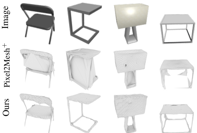
Figure 6. Pixel2Mesh+ predicts meshes by deforming an initial sphere, so it cannot properly model objects with holes. In contrast our method can model objects with arbitrary topologies.
图 6: Pixel2Mesh+ 通过变形初始球体来预测网格,因此无法正确建模带孔洞的物体。相比之下,我们的方法能够建模任意拓扑结构的物体。
Ablation Study Fairly comparing with prior work is challenging due to differences in backbone networks, losses, and shape regularize rs. For a controlled evaluation, we ablate variants using the same backbone and training recipe, shown in Table 2. ShapeNet is dominated by simple objects of genus zero. Therefore we evaluate both on the entire test set and on a subset consisting of objects with one or more holes (Holes Test Set) 2. In this evaluation we remove the ad-hoc scaling factor of 0.57, and we rescale meshes so the longest edge of the ground-truth mesh’s bounding box has length 10, following [8]. We compare the open-source
消融实验
由于主干网络、损失函数和形状正则化器的差异,与先前工作进行公平比较具有挑战性。为进行可控评估,我们采用相同主干网络和训练方案对变体进行消融实验,如表 2 所示。ShapeNet 主要由零亏格的简单物体主导,因此我们同时在完整测试集和包含一个或多个孔洞的物体子集 (Holes Test Set) 上进行评估。本评估遵循 [8] 的方法,移除了 0.57 的临时缩放因子,并将网格重新缩放至真实网格包围盒的最长边长度为 10。我们比较了开源...
Table 3. Performance on Pix3D $S_{1}$ & $S_{2}$ . We report mean $\mathrm{AP^{box}}$ , $\mathbf{AP}^{\mathrm{mask}}$ and $\mathbf{AP}^{\mathrm{mesh}}$ , as well as per category $\mathbf{AP}^{\mathrm{mesh}}$ . All AP performances are in $%$ . The Voxel-Only baseline outputs the cubified voxel predictions. The Sphere-Init and $P i x e l2M e s h^{+}$ baselines deform an initial sphere and thus are limited to making predictions homeomorphic to spheres. Our Mesh R-CNN is flexible and can capture arbitrary topologies. We outperform the baselines consistently while predicting meshes with fewer number of vertices and faces.
表 3: Pix3D $S_{1}$ 和 $S_{2}$ 上的性能表现。我们报告了平均 $\mathrm{AP^{box}}$、$\mathbf{AP}^{\mathrm{mask}}$ 和 $\mathbf{AP}^{\mathrm{mesh}}$,以及每个类别的 $\mathbf{AP}^{\mathrm{mesh}}$。所有 AP 性能均以 $%$ 表示。Voxel-Only 基线输出立方体化的体素预测。Sphere-Init 和 $P i x e l2M e s h^{+}$ 基线通过变形初始球体生成预测,因此仅限于生成与球体同胚的预测结果。我们的 Mesh R-CNN 具有灵活性,能够捕捉任意拓扑结构。在预测顶点和面数更少的网格时,我们的方法始终优于基线模型。
| Pix3D S1 | APbox | Apmask | Apmesh | chair | sofa | table | bed | desk | bkcs | wrdrb | tool | misc | [V] | F] |
|---|---|---|---|---|---|---|---|---|---|---|---|---|---|---|
| Voxel-Only | 94.4 | 88.4 | 5.3 | 0.0 | 3.5 | 2.6 | 0.5 | 0.7 | 34.3 | 5.7 | 0.0 | 0.0 | 2354±706 | 4717±1423 |
| Pixel2Mesh+ | 93.5 | 88.4 | 39.9 | 30.9 | 59.1 | 40.2 | 40.5 | 30.2 | 50.8 | 62.4 | 18.2 | 26.7 | 2562±0 | 5120±0 |
| Sphere-Init | 94.1 | 87.5 | 40.5 | 40.9 | 75.2 | 44.2 | 50.3 | 28.4 | 48.6 | 42.5 | 26.9 | 7.0 | 2562±0 | 5120±0 |
| MeshR-CNN (ours) | 94.0 | 88.4 | 51.1 | 48.2 | 71.7 | 60.9 | 53.7 | 42.9 | 70.2 | 63.4 | 21.6 | 27.8 | 2367±698 | 4743±1406 |
| #test instances | 2530 | 2530 | 2530 | 1165 | 415 | 419 | 213 | 154 | 79 | 54 | 11 | 20 |
| Pix3D S2 | APbox | Apmask | Apmesh | chair | sofa | table | bed | desk | bkcs | wrdrb | tool | misc | [V] | F] |
|---|---|---|---|---|---|---|---|---|---|---|---|---|---|---|
| Voxel-Only | 71.5 | 63.4 | 4.9 | 0.0 | 0.1 | 2.5 | 2.4 | 0.8 | 32.2 | 0.0 | 6.0 | 0.0 | 2346±630 | 4702±1269 |
| Pixel2Mesh+ | 71.1 | 63.4 | 21.1 | 26.7 | 58.5 | 10.9 | 38.5 | 7.8 | 34.1 | 3.4 | 10.0 | 0.0 | 2562±0 | 5120±0 |
| Sphere-Init | 72.6 | 64.5 | 24.6 | 32.9 | 75.3 | 15.8 | 40.1 | 10.1 | 45.0 | 1.5 | 0.8 | 0.0 | 2562±0 | 5120±0 |
| MeshR-CNN (ours) | 72.2 | 63.9 | 28.8 | 42.7 | 70.8 | 27.2 | 40.9 | 18.2 | 51.1 | 2.9 | 5.2 | 0.0 | 2358±633 | 4726±1274 |
| #test instances | 2356 | 2356 | 2356 | 777 | 504 | 392 | 218 | 205 | 84 | 134 | 22 | 20 |
Table 4. Ablations of Mesh R-CNN on Pix3D.
表 4: Pix3D数据集上Mesh R-CNN的消融实验
| CNNinit | #refine steps | APbox | APmask | Apmesh |
|---|---|---|---|---|
| COCO | 3 | 94.0 | 88.4 | 51.1 |
| IN | 3 | 93.1 | 87.0 | 48.4 |
| COCO | 2 | 94.6 | 88.3 | 49.3 |
| COCO | 1 | 94.2 | 88.9 | 48.6 |
Pixel2Mesh model against our ablations in this evaluation setting. Pixel2Mesh+ (our re implementation of [69]) significantly outperforms the original due to an improved training recipe and deeper backbone.
Pixel2Mesh模型在本评估设置中与我们的消融实验对比。Pixel2Mesh+(我们对[69]的重新实现)由于改进了训练方案和更深的骨干网络,显著优于原始版本。
We draw several conclusions from Table 2: (a) On the Full Test Set, our full model and Pixel2Mesh+ perform on par. However, on the Holes Test Set, our model dominates as it is able to predict topologically diverse shapes while Pixel2Mesh+ is restricted to make predictions homeomorphic to spheres, and cannot model holes or disconnected components (see Figure 6). This discrepancy is quantitatively more salient on Pix3D (Section 4.2) as it contains more complex shapes. (b) Sphere-Init and Pixel2Mesh+ perform similarly overall (both Best and Pretty), suggesting that mesh subdivision may be unnecessary for strong quantitative performance. (c) The deeper residual mesh refinement architecture (inspired by [69]) performs on-par with the lighter non-residual architecture, motivating our use of the latter on Pix3D. (d) Voxel-Only performs poorly compared to methods that predict meshes, demonstrating that mesh predictions better capture fine object structure. (e) Each Best model outperforms its corresponding Pretty model; this is expected since Best is an upper bound on quantitative performance.
从表2可以得出以下几点结论:(a) 在完整测试集(Full Test Set)上,我们的完整模型与Pixel2Mesh+表现相当。但在孔洞测试集(Holes Test Set)上,我们的模型占据优势,因为它能预测拓扑结构多样的形状,而Pixel2Mesh+仅限于预测与球面同胚的形状,无法建模孔洞或离散组件(见图6)。这种差异在Pix3D数据集(第4.2节)上更为显著,因其包含更复杂的形状。(b) Sphere-Init和Pixel2Mesh+整体表现相近(包括Best和Pretty版本),表明网格细分对于获得强劲的量化性能可能并非必要。(c) 更深的残差网格优化架构(受[69]启发)与更轻量的非残差架构表现相当,这促使我们在Pix3D上采用后者。(d) 与预测网格的方法相比,Voxel-Only表现较差,证明网格预测能更好地捕捉精细物体结构。(e) 每个Best模型都优于其对应的Pretty模型,这符合预期,因为Best代表量化性能的上限。
4.2. Pix3D
4.2. Pix3D
We now turn to Pix3D [60], which consists of 10069 real-world images and 395 unique 3D models. Here the task is to jointly detect and predict 3D shapes for known object categories. Pix3D does not provide standard train/test splits, so we prepare two splits of our own.
现在我们转向Pix3D [60],它包含10069张真实世界图像和395个独特的3D模型。这里的任务是联合检测并预测已知物体类别的3D形状。Pix3D未提供标准训练/测试划分,因此我们自行准备了两组划分。
Our first split, $S_{1}$ , randomly allocates 7539 images for training and 2530 for testing. Despite the small number of unique object models compared to ShapeNet, $S_{1}$ is challenging since the same model can appear with varying appearance (e.g. color, texture), in different orientations, under different lighting conditions, in different contexts, and with varying occlusion. This is a stark contrast with ShapeNet, where objects appear against blank backgrounds.
我们的第一个划分 $S_{1}$ 随机分配了7539张图像用于训练,2530张用于测试。尽管与ShapeNet相比,独特的物体模型数量较少,但 $S_{1}$ 具有挑战性,因为同一模型可能以不同的外观(例如颜色、纹理)、不同的方向、不同的光照条件、不同的背景以及不同程度的遮挡出现。这与ShapeNet形成鲜明对比,后者的物体出现在空白背景上。
Our second split, $S_{2}$ , is even more challenging: we ensure that the 3D models appearing in the train and test sets are disjoint. Success on this split requires generalization not only to the variations present in $S_{1}$ , but also to novel 3D shapes of known categories: for example a model may see kitchen chairs during training but must recognize armchairs during testing. This split is possible due to Pix3D’s unique annotation structure, and poses interesting challenges for both 2D recognition and 3D shape prediction.
我们的第二个划分 $S_{2}$ 更具挑战性:确保训练集和测试集中出现的3D模型互不重叠。在此划分上取得成功不仅需要泛化 $S_{1}$ 中的变化,还需适应已知类别的新颖3D形状:例如模型可能在训练时见过餐椅,但测试时必须识别扶手椅。这一划分得益于Pix3D独特的标注结构,为2D识别和3D形状预测都带来了有趣的挑战。
Evaluation We adopt metrics inspired by those used for 2D recognition: $\mathrm{AP^{box}}$ , $\mathrm{AP^{mask}}$ and $\mathrm{AP^{mesh}}$ . The first two are standard metrics used for evaluating COCO object detection and instance segmentation at intersection-over-union (IoU) 0.5. $\mathrm{AP^{mesh}}$ evalutes 3D shape prediction: it is the mean area under the per-category precision-recall curves for $\mathrm{F}1^{0.3}$ at $0.5^{3}$ . Pix3D is not exhaustively annotated, so for evaluation we only consider predictions with box $\mathrm{IoU}>0.3$ with a ground-truth region. This avoids penalizing the model for correct predictions corresponding to un annotated objects.
评估
我们采用了受2D识别启发的指标:$\mathrm{AP^{box}}$、$\mathrm{AP^{mask}}$和$\mathrm{AP^{mesh}}$。前两个是用于在交并比(IoU)0.5下评估COCO目标检测和实例分割的标准指标。$\mathrm{AP^{mesh}}$评估3D形状预测:它是$\mathrm{F}1^{0.3}$在$0.5^{3}$下每类别精确率-召回率曲线下面积的平均值。由于Pix3D未完全标注,因此评估时我们仅考虑与真实区域框$\mathrm{IoU}>0.3$的预测。这避免了因未标注对象对应的正确预测而惩罚模型。
We compare predicted and ground-truth meshes in the camera coordinate system. Our model assumes known camera intrinsics for VertAlign. In addition to predicting the box of each object on the image plane, Mesh R-CNN predicts the depth extent by appending a 2-layer MLP head, similar to the box regressor head. As a result, Mesh RCNN predicts a 3D bounding box for each object. See Appendix E for more details.
我们在相机坐标系下比较预测网格与真实网格。我们的模型假设已知相机内参用于VertAlign。除了预测图像平面上每个物体的边界框外,Mesh R-CNN还通过附加一个2层MLP头(类似于边界框回归头)来预测深度范围。因此,Mesh R-CNN会为每个物体预测一个3D边界框。更多细节参见附录E。

Figure 7. Examples of Mesh R-CNN predictions on Pix3D. Mesh R-CNN detects multiple objects per image, reconstructs fine details such as chair legs, and predicts varying and complex mesh topologies for objects with holes such as bookcases and tables.
图 7: Mesh R-CNN在Pix3D数据集上的预测示例。Mesh R-CNN能检测每张图像中的多个物体,重建精细细节(如椅子腿),并为带孔物体(如书架和桌子)预测多样且复杂的网格拓扑结构。
Implementation details We use ResNet-50-FPN [35] as the backbone CNN; the box and mask branches are identical to Mask R-CNN. The voxel branch resembles the mask branch, but the pooling resolution is decreased to 12 (vs. 14 for masks) due to memory constraints giving $24\times24\times24$ voxel predictions. We adopt the lightweight design for the mesh refinement branch from Section 4.1. We train for 12 epochs with a batch size of 64 per image on 8 Tesla V100 GPUs (two images per GPU). We use SGD with momentum, linearly increasing the learning rate from 0.002 to 0.02 over the first 1K iterations, then decaying by a factor of 10 at 8K and 10K iterations. We initialize from a model pretrained for instance segmentation on COCO. We set the cubify threshold to 0.2 and the loss weights to $\lambda_{\mathrm{voxel}}=3$ , $\lambda_{\mathrm{cham}}=1$ , $\lambda_{\mathrm{norm}}=0.1$ and $\lambda_{\mathrm{edge}}=1$ and use weight decay $10^{-4}$ ; detection loss weights are identical to Mask R-CNN.
实现细节
我们采用ResNet-50-FPN [35]作为主干CNN;边界框和掩码分支与Mask R-CNN相同。体素分支类似掩码分支,但由于内存限制将池化分辨率降至12(掩码为14),生成$24\times24\times24$的体素预测。网格优化分支采用第4.1节的轻量化设计。在8块Tesla V100 GPU上训练12个周期(每GPU处理2张图像),批次大小为64。使用带动量的SGD优化器,前1K次迭代中学习率从0.002线性增至0.02,随后在8K和10K次迭代时衰减10倍。模型初始化权重来自COCO实例分割预训练模型。设置立方化阈值为0.2,损失权重为$\lambda_{\mathrm{voxel}}=3$、$\lambda_{\mathrm{cham}}=1$、$\lambda_{\mathrm{norm}}=0.1$和$\lambda_{\mathrm{edge}}=1$,权重衰减为$10^{-4}$;检测损失权重与Mask R-CNN一致。
Comparison to Baselines As discussed in Section 1, we are the first to tackle joint detection and shape inference in the wild on Pix3D. To validate our approach we compare with ablated versions of Mesh R-CNN, replacing our full mesh predictor with Voxel-Only, $P i x e l2M e s h^{+}$ , and SphereInit branches (see Section 4.1). All baselines otherwise use the same architecture and training recipe.
与基线对比
如第1节所述,我们是首个在Pix3D数据集上实现野外联合检测与形状推断的方法。为验证本方法,我们与Mesh R-CNN的消融版本进行对比:将完整网格预测器替换为仅体素分支 (Voxel-Only) 、$Pixel2Mesh^{+}$分支及球面初始化分支 (SphereInit) (见4.1节)。所有基线模型均采用相同架构与训练方案。
Table 3 (top) shows the performance on $S_{1}$ . We observe that: (a) Mesh R-CNN outperforms all baselines, improving over the next-best by $10.6%$ APmesh overall and across most categories; Tool and $M i s c^{4}$ have very few test-set instances (11 and 20 respectively), so their AP is noisy. (b) Mesh R-CNN shows large gains vs. Sphere-Init for objects with complex shapes such as bookcase $(+21.6%)$ , table $(+16.7%)$ and chair $(+7.3%)$ . (c) Voxel-Only performs very poorly – this is expected due to its coarse predictions.
表 3 (上)展示了在 $S_{1}$ 上的性能表现。我们观察到:(a) Mesh R-CNN在所有基线方法中表现最优,整体APmesh比次优方法提高了 $10.6%$ ,且在大多数类别中都有提升;Tool和 $M i s c^{4}$ 的测试集实例非常少(分别为11和20个),因此它们的AP值存在较大噪声。(b) 对于书柜 $(+21.6%)$ 、桌子 $(+16.7%)$ 和椅子 $(+7.3%)$ 等形状复杂的物体,Mesh R-CNN相比Sphere-Init展现出显著优势。(c) Voxel-Only方法表现非常差,这与其粗糙的预测结果相符。
Table 3 (bottom) shows the performance on the more challenging $S_{2}$ split. Here we observe: (a) The overall performance on 2D recognition $(\mathrm{AP}^{\mathrm{box}}$ , $\mathrm{AP^{mask}}$ ) drops significantly compared to $S_{1}$ , signifying the difficulty of recognizing novel shapes in the wild. (b) Mesh R-CNN outperforms all baselines for shape prediction for all categories except sofa, wardrobe and tool. (c) Absolute performance on wardrobe, tool and misc is small for all methods due to significant shape disparity between models in train and test and lack of training data.
表 3 (底部)展示了更具挑战性的 $S_{2}$ 分割上的性能表现。我们观察到: (a) 与 $S_{1}$ 相比, 2D识别性能 $(\mathrm{AP}^{\mathrm{box}}$, $\mathrm{AP^{mask}}$) 显著下降, 这表明在自然场景中识别新形状的难度较大。 (b) 除沙发、衣柜和工具类别外, Mesh R-CNN在所有类别的形状预测上都优于所有基线方法。 (c) 由于训练集和测试集中模型形状差异较大且缺乏训练数据, 所有方法在衣柜、工具和杂项类别上的绝对性能都较低。

Figure 8. More examples of Mesh R-CNN predictions on Pix3D.
图 8: Pix3D数据集上Mesh R-CNN预测的更多示例
Table 4 compares pre training on COCO vs ImageNet, and compares different architectures for the mesh predictor. COCO vs. ImageNet initialization improves 2D recognition $(\mathrm{AP^{mask}88.4\nu s.87.0})$ and 3D shape prediction (APmesh 51.1 vs. 48.4). Shape prediction is degraded when using only one mesh refinement stage (APmesh 51.1 vs. 48.6).
表 4 比较了在 COCO 和 ImageNet 上的预训练效果,以及不同网格预测架构的差异。使用 COCO 初始化相比 ImageNet 提升了 2D 识别性能 $(\mathrm{AP^{mask}88.4\nu s.87.0})$ 和 3D 形状预测 (APmesh 51.1 vs. 48.4)。当仅使用单阶段网格优化时,形状预测性能会下降 (APmesh 51.1 vs. 48.6)。
Figures 2, 7 and 8 show example predictions from Mesh R-CNN. Our method can detect multiple objects per image, reconstruct fine details such as chair legs, and predict varying and complex mesh topologies for objects with holes such as bookcases and desks.
图 2、图 7 和图 8 展示了 Mesh R-CNN 的预测示例。我们的方法能在单张图像中检测多个物体,重建精细细节(如椅腿),并为书桌、书架等带孔物体预测多样化且复杂的网格拓扑结构。
Discussion
讨论
We propose Mesh R-CNN, a novel system for joint 2D perception and 3D shape inference. We validate our approach on ShapeNet and show its merits on Pix3D. Mesh R-CNN is a first attempt at 3D shape prediction in the wild. Despite the lack of large supervised data, e.g. compared to COCO, Mesh R-CNN shows promising results. Mesh RCNN is an object centric approach. Future work includes reasoning about the 3D layout, i.e. the relative pose of objects in the 3D scene.
我们提出了Mesh R-CNN,一个用于联合2D感知与3D形状推断的新颖系统。我们在ShapeNet上验证了该方法,并在Pix3D上展示了其优势。Mesh R-CNN是首个针对真实场景下3D形状预测的尝试。尽管缺乏大规模监督数据(例如与COCO相比),Mesh R-CNN仍显示出有前景的结果。Mesh R-CNN是一种以物体为中心的方法。未来工作包括对3D布局(即3D场景中物体的相对位姿)进行推理。
Acknowledgements We would like to thank Kaiming He, Piotr Dollar, Leonidas Guibas, Manolis Savva and Shubham Tulsiani for valuable discussions. We would also like to thank Lars Mescheder and Thibault Groueix for their help.
致谢
我们要感谢 Kaiming He、Piotr Dollar、Leonidas Guibas、Manolis Savva 和 Shubham Tulsiani 提供的宝贵讨论。同时感谢 Lars Mescheder 和 Thibault Groueix 的帮助。
Appendix
附录
B. Mesh Sampling
B. 网格采样
A. Implementation of Cubify
A. Cubify 的实现
Algorithm 1 outlines the cubify operation. Cubify takes as input voxel occupancy probabilities $V$ of shape $N\times D\times H\times W$ as predicted from the voxel branch and a threshold value $\tau$ . Each occupied voxel is replaced with a cuboid triangle mesh (unit cube) with 8 vertices, 18 edges, and 12 faces. Shared vertices and edges between adjacent occupied voxels are merged, and shared interior faces are eliminated. This results in a watertight mesh $T=(V,F)$ for each example in the batch whose topology depends on the voxel predictions.
算法1概述了立方化操作。立方化以体素分支预测的形状为 $N\times D\times H\times W$ 的体素占用概率 $V$ 和阈值 $\tau$ 作为输入。每个被占用的体素替换为一个具有8个顶点、18条边和12个面的立方体三角网格(单位立方体)。相邻被占用体素之间的共享顶点和边会被合并,共享内部面会被消除。这会为批次中的每个样本生成一个水密网格 $T=(V,F)$,其拓扑结构取决于体素预测结果。
Algorithm 1 is an inefficient implementation of cubify as it involves nested for loops which in practice increase the time complexity, especially for large batches and large voxel sizes. In particular, this implementation takes $>300\mathrm{ms}$ for $N=32$ voxels of size $32\times32\times32$ on aTesla V100 GPU. We replace the nested for loops with 3D convolutions and vectorize our computations, resulting in a time complexity of $\approx30\mathrm{ms}$ for the same voxel inputs.
算法1是cubify的一种低效实现,因为它涉及嵌套for循环,这在实际应用中会增加时间复杂度,特别是对于大批量和大体素尺寸的情况。具体来说,在Tesla V100 GPU上,对于尺寸为$32\times32\times32$的$N=32$个体素,此实现耗时$>300\mathrm{ms}$。我们用3D卷积替换了嵌套for循环并向量化计算,使得相同体素输入的耗时降至$\approx30\mathrm{ms}$。
As described in the main paper, the mesh refinement head is trained to minimize chamfer and normal losses that are defined on sets of points sampled from the predicted and ground-truth meshes.
如主论文所述,网格优化头的训练目标是最小化倒角距离和法向损失,这些损失函数基于从预测网格和真实网格采样得到的点集定义。
Computing these losses requires some method of converting meshes into sets of sampled points. Pixel2Mesh [69] is trained using similar losses. In their case groundtruth meshes are represented with points sampled uniformly at random from the surface of the mesh, but this sampling is performed offline before the start of training; they represent predicted meshes using their vertex positions. Computing these losses using vertex positions of predicted meshes is very efficient since it avoids the need to sample meshes online during training; however it can lead to degenerate predictions since the loss would not encourage the interior of predicted faces to align with the ground-truth mesh.
计算这些损失需要某种将网格转换为采样点集的方法。Pixel2Mesh [69] 使用类似的损失进行训练。在他们的方法中,真实网格通过从网格表面均匀随机采样的点来表示,但这种采样是在训练开始前离线完成的;他们使用顶点位置来表示预测网格。通过预测网格的顶点位置计算这些损失非常高效,因为它避免了在训练期间在线采样网格的需要;然而,这可能导致预测退化,因为损失不会促使预测面的内部与真实网格对齐。
To avoid these potential de genera cie s, we follow [57] and compute the chamfer and normal losses by randomly sampling points from both the predicted and ground-truth meshes. This means that we need to sample the predicted meshes online during training, so the sampling must be efficient and we must be able to back propagate through the sampling procedure to propagate gradients backward from the sampled points to the predicted vertex positions.
为避免这些潜在的退化问题,我们遵循[57]的方法,通过从预测网格和真实网格中随机采样点来计算倒角距离(chamfer)和法向损失(normal)。这意味着我们需要在训练过程中在线采样预测网格,因此采样必须高效,并且必须能够通过采样过程反向传播梯度,将梯度从采样点传播回预测的顶点位置。
Given a mesh with vertices $V\subset\mathbb{R}^{3}$ and faces $F\subseteq$ $V\times V\times V$ , we can sample a point uniformly from the surface of the mesh as follows. We first define a probability distribution over faces where each face’s probability is proportional to its area:
给定一个顶点集 $V\subset\mathbb{R}^{3}$ 和面集 $F\subseteq V\times V\times V$ 的网格,我们可以按以下步骤从其表面均匀采样一个点。首先定义一个基于面面积的概率分布:
$$
P(f)={\frac{a r e a(f)}{\sum_{f^{\prime}\in F}a r e a(f^{\prime})}}
$$
$$
P(f)={\frac{a r e a(f)}{\sum_{f^{\prime}\in F}a r e a(f^{\prime})}}
$$
We then sample a face $f=(v_{1},v_{2},v_{3})$ from this distribution. Next we sample a point $p$ uniformly from the interior of $f$ by setting $p=\textstyle\sum_{i}w_{i}v_{i}$ where $w_{1}=1-\sqrt{\xi_{1}}$ , $w_{2}=(1-\xi_{2})\sqrt{\xi}_{1}$ , $w_{3}=\xi_{2}\sqrt{\xi}_{1}$ , and $\xi_{1},\xi_{2}\sim U(0,1)$ are sampled from a uniform distribution.
然后从这个分布中采样一个面 $f=(v_{1},v_{2},v_{3})$。接着通过设置 $p=\textstyle\sum_{i}w_{i}v_{i}$ 从 $f$ 的内部均匀采样一个点 $p$,其中 $w_{1}=1-\sqrt{\xi_{1}}$,$w_{2}=(1-\xi_{2})\sqrt{\xi}_{1}$,$w_{3}=\xi_{2}\sqrt{\xi}_{1}$,且 $\xi_{1},\xi_{2}\sim U(0,1)$ 是从均匀分布中采样的。
This formulation allows propagating gradients from $p$ backward to the face vertices $v_{i}$ and can be seen as an instance of the re parameter iz ation trick [28].
该公式允许将梯度从 $p$ 反向传播到面部顶点 $v_{i}$,可视为重参数化技巧 [28] 的一个实例。
C. Mesh R-CNN Architecture
C. Mesh R-CNN 架构
At a high level we use the same overall architecture for predicting meshes on ShapeNet and Pix3D, but we slightly specialize to each dataset due to memory constraints from the backbone and task-specific heads. On Pix3D Mask RCNN adds time and memory complexity in order to perform object detection and instance segmentation.
从高层次来看,我们在ShapeNet和Pix3D上使用相同的整体架构来预测网格,但由于主干网络和任务特定头部的内存限制,我们对每个数据集进行了轻微调整。在Pix3D上,Mask RCNN为了执行目标检测和实例分割增加了时间和内存复杂度。
ShapeNet. The overall architecture of our ShapeNet model is shown in Table 6; the architecture of the voxel branch is shown in Table 8.
ShapeNet。我们的ShapeNet模型整体架构如表6所示;体素分支的架构如表8所示。
Table 5. Architecture for a single residual mesh refinement stage on ShapeNet. For ShapeNet we follow [69] and use residual blocks of graph convolutions: Res Graph Con v $'D_{1}\rightarrow D_{2}$ ) consists of two graph convolution layers (each preceeded by ReLU) and an additive skip connection, with a linear projection if the input and output dimensions are different. The output of the refinement stage are the vertex features (15) and the updated vertex positions (18). The first refinement stage does not take input vertex features (5), so for this stage (13) only concatenates (6) and (12).
表 5. ShapeNet上单阶段残差网格细化的架构。对于ShapeNet,我们遵循[69]并使用图卷积的残差块:Res Graph Conv ( $'D_{1}\rightarrow D_{2}$ ) 包含两个图卷积层(每个层前都有ReLU)和一个加法跳跃连接,如果输入和输出维度不同则使用线性投影。细化阶段的输出是顶点特征(15)和更新后的顶点位置(18)。第一个细化阶段不接收输入顶点特征(5),因此在此阶段(13)仅拼接(6)和(12)。
| 索引 | 输入 | 操作 | 输出形状 |
|---|---|---|---|
| (1) | 输入 | conv2_3特征 | 35×35×256 |
| (2) | 输入 | conv3_4特征 | 18×18×512 |
| (3) | 输入 | conv4_6特征 | 9×9×1024 |
| (4) | 输入 | conv5_3特征 | 5×5×2048 |
| (5) | 输入 | 输入顶点特征 | [V |
| (6) | 输入 | 输入顶点位置 | [V |
| (7) | (1), (6) | VertAlign | [V |
| (8) | (2), (6) | VertAlign | [V |
| (9) | (3), (6) | VertAlign | [V |
| (10) | (4), (6) | VertAlign | [V |
| (11) | (7),(8),(9),(10) | 拼接 | [V |
| (12) (13) | (11) | Linear(3840→128) | [V |
| (14) | (5),(6),(12) | 拼接 | [V |
| (13) | ResGraphConv(259→128) | [V | |
| (15) | (14) | 2×ResGraphConv(128→128) | [V |
| (16) | (15) | GraphConv(128→3) | [V |
| (17) | (16) | Tanh | [V |
| (18) | (6), (17) | 加法 | [V |
Table 6. Overall architecture for our ShapeNet model. Since we do not predict bounding boxes or masks, we feed the $\mathtt{C O n v5}_{-3}$ features from the whole image into the voxel branch. The architecture for the refinement stage is shown in Table 5, and the architecture for the voxel branch is shown in Table 8.
表 6. 我们的ShapeNet模型整体架构。由于不预测边界框或掩码,我们将整张图像的$\mathtt{C O n v5}_{-3}$特征输入到体素分支。细化阶段的架构如 表 5 所示,体素分支的架构如 表 8 所示。
| 序号 | 输入 | 操作 | 输出形状 |
|---|---|---|---|
| (1) | Input | Image | 137×137×3 |
| (2) | ResNet-50conv2_3 | 35×35×256 | |
| (3) | ResNet-50conv3_4 | 18×18×512 | |
| (4) | ResNet-50conv4_6 | 9×9×1024 | |
| (5) | ResNet-50conv5-3 | Bilinear interpolation VoxelBranch cubify | 5×5×2048 24×24×2048 48×48×48 |
| (6) | V |
We consider two different architectures for the mesh refinement network on ShapeNet. Our full model as well as our Pixel2Mesh+ and Sphere-Init baselines use mesh refinement stages with three residual blocks of two graph convolutions each, similar to [69]; the architecture of these stages is shown in Table 5. We also consider a shallower lightweight design which uses only three graph convolution layers per stage, omitting residual connections and instead concatenating the input vertex positions before each graph convolution layer. The architecture of this lightweight design is shown in Table 7.
我们在ShapeNet上考虑了两种不同的网格细化网络架构。我们的完整模型以及Pixel2Mesh+和Sphere-Init基线采用类似[69]的三阶段残差块设计,每个阶段包含两个图卷积层,具体架构如表5所示。同时,我们还测试了一种更轻量的浅层设计,每个阶段仅使用三个图卷积层,省略残差连接,改为在每个图卷积层前拼接输入顶点坐标,该轻量架构如表7所示。
As shown in Table 2, we found that these two architectures perform similarly on ShapeNet even though the lightweight design uses half as many graph convolution layers per stage. We therefore use the non residual design for our Pix3D models.
如表 2 所示,我们发现这两种架构在 ShapeNet 上的表现相似,尽管轻量级设计每个阶段使用的图卷积层数量减半。因此,我们为 Pix3D 模型采用了非残差设计。
Table 7. Architecture for the non residual mesh refinement stage use in the lightweight version of our ShapeNet models. Each GraphConv operation is followed by ReLU. The output of the stage are the vertex features (18) and updated vertex positions (21). The first refinement stage does not take input vertex features (5), so for this stage (13) only concatenates (6) and (12).
表 7. 轻量级ShapeNet模型中使用的非残差网格细化阶段架构。每个GraphConv操作后接ReLU激活。该阶段输出顶点特征(18)和更新后的顶点位置(21)。首个细化阶段不接收输入顶点特征(5),因此该阶段的(13)仅拼接(6)和(12)。
| 序号 | 输入 | 操作 | 输出形状 |
|---|---|---|---|
| (1) | Input | conv2_3features | 35×35×256 |
| (2) | Input | conv3_4features | 18×18×512 |
| (3) | Input | conv4_6features | 9×9×1024 |
| (4) | Input | conv5_3features | 5×5×2048 |
| (5) | Input | Inputvertexfeatures | [V |
| (6) | Input | Input vertex positions | |
| (7) | (1), (6) | VertAlign | [V |
| (8) | (2), (6) | VertAlign | |
| (9) | (3), (6) | VertAlign | |
| (10) | (4), (6) | VertAlign | |
| (11) | (7),(8),(9),(10) | Concatenate | |
| (12) | (11) | Linear(3840→128) | [V |
| (13) | (5), (6), (12) | Concatenate | |
| (14) | (13) | GraphConv(259→128) | [V |
| (15) | (6), (14) | Concatenate | [V |
| (16) | (15) | GraphConv(131→128) | [V |
| (17) | (6), (16) | Concatenate | [V |
| (18) | (17) | GraphConv(131→128) | [V |
| (19) | (18) | Linear(128→3) | [V |
| (20) | (19) | Tanh | |
| (21) | (6), (20) | Addition |
Table 8. Architecture of our voxel prediction branch. For ShapeNet we use $V=48$ and for Pix3D we use $V=24$ . TConv is a transpose convolution with stride 2.
表 8: 我们的体素预测分支架构。对于 ShapeNet 我们使用 $V=48$,对于 Pix3D 我们使用 $V=24$。TConv 是步长为 2 的转置卷积。
| 索引 | 输入 | 操作 | 输出形状 |
|---|---|---|---|
| (1) (2) (3) | 输入 (1) | 图像特征 Conv(D→256,3×3),ReLU Conv(256→256,3×3),ReLU | V/2×V/2×D V/2xV/2×256 V/2xV/2×256 |
Pix3D. The overall architecture of our full Mesh R-CNN system on Pix3D is shown in Table 9. The backbone, RPN, box branch, and mask branch are identical to Mask RCNN [18]. The voxel branch is the same as in the ShapeNet models (see Table 8), except that we predict voxels at a lower resolution $(48\times48\times48$ for ShapeNet vs. $24\times24\times24$ for Pix3D) due to memory constraints. Table 10 shows the exact architecture of the mesh refinement stages for our Pix3D models.
Pix3D。我们在Pix3D上的完整Mesh R-CNN系统整体架构如表9所示。主干网络(backbone)、区域提议网络(RPN)、边界框分支(box branch)和掩码分支(mask branch)与Mask RCNN [18]相同。体素分支(voxel branch)与ShapeNet模型中的结构一致(见表8),但由于内存限制,我们预测的体素分辨率较低(ShapeNet为$(48\times48\times48$,Pix3D为$24\times24\times24$)。表10展示了Pix3D模型的网格细化阶段具体架构。
Baselines. The Voxel-Only baseline is identical to the full model, except that it omits all mesh refinement branches and terminates with the mesh resulting from cubify. On ShapeNet, the Voxel-Only baseline is trained with a batch size of 64 (vs. a batch size of 32 for our full model); on Pix3D it uses the same training recipe as our full model.
基线。Voxel-Only基线模型与完整模型结构相同,仅移除了所有网格优化分支,最终输出由立方体化(cubify)生成的初始网格。在ShapeNet数据集上,Voxel-Only基线采用64的批处理规模(完整模型为32);在Pix3D数据集上则采用与完整模型相同的训练方案。
The Pixel2Mesh+ is our re implementation of [69]. This baseline omits the voxel branch; instead all images use an identical inital mesh. The initial mesh is a level-2 icosphere
Pixel2Mesh+是我们对[69]的重新实现。该基线方法省略了体素分支,所有图像均使用相同的初始网格。初始网格为二级二十面体。
| 序号 | 输入操作 | 输出形状 | |
|---|---|---|---|
| (1) | 输入 | 输入图像 | H×W×3 |
| (2) | (1) | 主干网络: ResNet-50-FPN | h×w×256 |
| (3) | (2) | RPN | h×w×A×4 |
| (4) | (2), (3) | RoIAlign | 14×14×256 |
| (5) | (4) | 边界框分支: 2×降采样, 展平, 线性层(77256→1024), 线性层(1024→5C) | C×5 |
| (6) | (4) | 掩码分支: 4×卷积(256→256,3×3), 转置卷积(256→256,2×2,2), 卷积(256→C,1×1) | 28×28×C |
| (7) | (2), (3) | RoIAlign | 12×12×256 |
| (8) | (7) | 体素分支 | 24×24×24 |
| (9) | (8) | 立方化 | V×3, |F|×3 |
| (10) | (7), (9) | 优化阶段1 | V×3, |F|×3 |
| (11) | (7), (10) | 优化阶段2 | V×3, |F|×3 |
| (12) | (7), (11) | 优化阶段3 | V×3, F×3 |
Table 9. Overall architecture of Mesh R-CNN on Pix3D. The backbone, RPN, box, and mask branches are identical to Mask R-CNN. The RPN produces a bounding box prediction for each of the $A$ anchors at each spatial location in the input feature map; a subset of these candidate boxes are processed by the other branches, but here we show only the shapes resulting from processing a single box for the subsequent task-specific heads. Here $C$ is the number of categories ( $10=9+$ background for Pix3D); the box branch produces per-category bounding boxes and classification scores, while the mask branch produces per-category segmentation masks. TConv is a transpose convolution with stride 2. We use a ReLU non linearity between all Linear, Conv, and TConv operations. The architecture fo the voxel branch is shown in Table 8, and the architecture of the refinement stages is shown in Table 10.
表 9: Pix3D 上 Mesh R-CNN 的整体架构。主干网络 (backbone)、RPN、边界框 (box) 和掩码 (mask) 分支与 Mask R-CNN 相同。RPN 为输入特征图中每个空间位置的 $A$ 个锚点 (anchor) 生成边界框预测;这些候选框的子集会由其他分支处理,但此处我们仅展示处理单个框后针对后续任务特定头 (task-specific head) 的形状结果。其中 $C$ 表示类别数量 (Pix3D 中 $10=9+$ 背景);边界框分支生成每个类别的边界框和分类分数,而掩码分支生成每个类别的分割掩码。TConv 是步长为 2 的转置卷积 (transpose convolution)。我们在所有线性 (Linear)、卷积 (Conv) 和转置卷积 (TConv) 操作之间使用 ReLU 非线性激活。体素 (voxel) 分支的架构如表 8 所示,细化阶段 (refinement stage) 的架构如表 10 所示。
Table 10. Architecture for a single mesh refinement stage on Pix3D.
| 序号 | 输入 | 操作 | 输出形状 |
|---|---|---|---|
| (1) (2) (3) (4) (5) (6) (7) (8) (9) (10) | 输入 输入 输入 (1), (3) (2),(3), (4) (5) (3), (6) (7) (3), (8) (9) (3), (10) | 主干特征 输入顶点特征 输入顶点位置 VertAlign 拼接 GraphConv(387→128) 拼接 GraphConv(131→128) 拼接 | h×w×256 [V]×128 [V]×3 |
表 10: Pix3D数据集上单次网格细化阶段的架构。
with 162 vertices, 320 faces, and 480 edges which results from applying two face subdivision operations to a regular icosahedron and projecting all resulting vertices onto a sphere. For the Pixel2Mesh+ baseline, the mesh refinement stages are the same as our full model, except that we apply a face subdivision operation prior to VertAlign in refinement stages 2 and 3.
包含162个顶点、320个面和480条边,这是对正二十面体进行两次面细分操作并将所有生成顶点投影到球面上的结果。对于Pixel2Mesh+基线,其网格细化阶段与我们完整模型相同,区别在于我们在第2和第3细化阶段的VertAlign操作前会先执行一次面细分操作。
Like Pixel2Mesh+, the Sphere-Init baseline omits the voxel branch and uses an identical initial sphere mesh for all images. However unlike Pixel2Mesh+ the initial mesh is a level-4 icosphere with 2562 vertices, 5120 faces, and 7680 edges which results from applying four face sub div iv is on operations to a regular icosahedron. Due to this large initial mesh, the mesh refinement stages are identical to our full model, and do not use mesh subdivision.
与Pixel2Mesh+类似,Sphere-Init基线省略了体素分支,并为所有图像使用相同的初始球面网格。但与Pixel2Mesh+不同的是,初始网格是一个具有2562个顶点、5120个面和7680条边的4级二十面体网格,这是通过对正二十面体进行四次面细分操作得到的。由于初始网格较大,网格细化阶段与我们的完整模型相同,且不使用网格细分。
Pixel2Mesh+ and Sphere-Init both predict meshes with the same number of vertices and faces, and with identical topologies; the only difference between them is whether all subdivision operations are performed before the mesh refinement branch (Sphere-Init) or whether mesh refinement is interleaved with mesh subdivision $\mathbf{(Pixel2Mesh^{+}}$ ). On ShapeNet, the Pixel2Mesh+ and Sphere-Init baselines are trained with a batch size of 96; on Pix3D they use the same training recipe as our full model.
Pixel2Mesh+ 和 Sphere-Init 都预测具有相同顶点数和面数、且拓扑结构完全一致的网格;它们之间的唯一区别在于所有细分操作是在网格优化分支之前全部完成 (Sphere-Init) ,还是将网格优化与网格细分交替进行 $\mathbf{(Pixel2Mesh^{+}}$ ) 。在 ShapeNet 上,Pixel2Mesh+ 和 Sphere-Init 基线模型的训练批次大小为 96;在 Pix3D 数据集上,它们采用与我们完整模型相同的训练方案。
Table 11. Comparison between our method and Occpancy Networks (OccNet) [42] on ShapeNet. We use the same evaluation metrics and setup as Table 2.
表 11. 我们的方法与Occpancy Networks (OccNet) [42]在ShapeNet上的对比。我们采用与表2相同的评估指标和设置。
| Chamfer(↓) | Normal | F10.1 | F10.3 | F10.5 | [V] | [F] | ||
|---|---|---|---|---|---|---|---|---|
| OccNet[42] | 0.264 | 0.789 | 33.4 | 80.5 | 91.3 | 2499±60 | 4995±120 | |
| est B | Ours (light) | 0.135 | 0.725 | 38.9 | 86.7 | 95.0 | 1978±951 | 3958±1906 |
| Ours | 0.139 | 0.728 | 38.3 | 86.3 | 94.9 | 1985±960 | 3971±1924 | |
| Ours (light) | 0.185 | 0.696 | 34.3 | 82.0 | 92.8 | 1976±956 | 3954±1916 | |
| Pretty | Ours | 0.180 | 0.709 | 34.6 | 82.2 | 93.0 | 1982±961 | 3967±1926 |
D. Comparison with Occupancy Networks
D. 与 Occupancy Networks 的对比
Occupancy Networks [42] (OccNet) also predict 2D meshes with neural networks. Rather than outputing a mesh directly from the neural network as in our approach, they train a neural network to compute a signed distance between a query point in 3D space and the object boundary. At testtime a 3D mesh can be extracted from a set of query points. Like our approach, OccNets can also predict meshes with varying topolgy per input instance.
占用网络 [42] (OccNet) 同样使用神经网络预测二维网格。与我们的方法直接从神经网络输出网格不同,他们训练神经网络来计算三维空间中查询点与物体边界的带符号距离。在测试阶段,可以从一组查询点中提取出三维网格。与我们的方法类似,OccNet 也能针对每个输入实例预测具有不同拓扑结构的网格。
Table 11 compares our approach with OccNet on the ShapeNet test set. We obtained test-set predictions for OccNet from the authors. Our method and OccNet are trained on slightly different splits of the ShapeNet dataset, so we compare our methods on the intersection of our respective test splits. From Table 11 we see that OccNets achieve higher normal consistency than our approach; however both the Best and Pretty versions of our model outperform OccNets on all other metrics.
表 11 将我们的方法与 OccNet 在 ShapeNet 测试集上进行了比较。我们从 OccNet 作者处获得了测试集预测结果。我们的方法与 OccNet 在 ShapeNet 数据集上使用了略有不同的划分方式,因此我们在双方测试集划分的交集上进行比较。从表 11 可以看出,OccNet 在法线一致性指标上优于我们的方法;但无论是 Best 还是 Pretty 版本的模型,在其他所有指标上均超越了 OccNet。
E. Depth Extent Prediction
E. 深度范围预测
Predicting an object’s depth extent from a single image is an ill-posed problem. In an earlier version of our work, we assumed the range of an object in the $Z$ -axis was given at train & test time. Since then, we have attempted to predict the depth extent by training a 2-layer MLP head of similar architecture to the bounding box regressor head. Formally, this head is trained to predict the scale-normalized depth extent (in log space) of the object, as follows
从单张图像预测物体的深度范围是一个不适定问题。在我们工作的早期版本中,我们假设物体在 $Z$ 轴上的范围在训练和测试时是已知的。此后,我们尝试通过训练一个与边界框回归头结构相似的2层MLP头来预测深度范围。具体而言,该头被训练用于预测物体经过尺度归一化(对数空间)的深度范围,如下所示
$$
\bar{d z}=\frac{d z}{z_{c}}\cdot\frac{f}{h}
$$
$$
\bar{d z}=\frac{d z}{z_{c}}\cdot\frac{f}{h}
$$
Note that the depth extent of an object is related to the size of the object (here approximated by the object’s bounding box height $h$ ), its location $z_{c}$ in the $Z$ -axis (far away objects need to be bigger in order to explain the image) and the focal length $f$ . At inference time the depth extent $d z$ of the object is recovered from the predicted d¯z and the predicted height of the object bounding box $h$ , given the focal length $f$ and the center of the object $z_{c}$ in the $Z$ -axis. Note that we assume the center of the object $z_{c}$ since Pix3D annotations are not metric and due to the inherent scale-depth ambiguity.
请注意,物体的深度范围与其大小(此处近似为物体边界框高度 $h$)、在 $Z$ 轴上的位置 $z_{c}$(远处的物体需要更大才能解释图像)以及焦距 $f$ 相关。在推理时,物体的深度范围 $dz$ 是根据预测的 $\bar{d}z$ 和物体边界框的预测高度 $h$ 恢复的,给定焦距 $f$ 和物体在 $Z$ 轴上的中心 $z{c}$。需要注意的是,由于 Pix3D 的标注不是度量值,且存在固有的尺度-深度模糊性,我们假设物体的中心为 $z_{c}$。
F. Pix3D: Visualization s and Comparisons
F. Pix3D: 可视化与对比
Figure 9 shows qualitative comparisons between $\mathrm{Pixel}2\mathbf{M}\mathrm{esh}^{+}$ and Mesh R-CNN. Pixel2Mesh+ is limited to making predictions homeomorphic to spheres and thus cannot capture varying topologies, e.g. holes. In addition, Pixel2Mesh+ has a hard time capturing high curvatures, such as sharp table tops and legs. This is due to the large deformations required when starting from a sphere, which are not encouraged by the shape regularize rs. On the other hand, Mesh R-CNN initializes its shapes with cubified voxel predictions resulting in better initial shape representations which require less drastic deformations.
图 9: 展示了 $\mathrm{Pixel}2\mathbf{M}\mathrm{esh}^{+}$ 与 Mesh R-CNN 的定性对比。Pixel2Mesh+ 的预测仅限于球面同胚结构,因此无法捕捉变化的拓扑特征(如孔洞)。此外,该模型难以还原高曲率几何(如尖锐的桌面和桌腿),这是因为从球体初始形态出发需要大幅形变,而形状正则化器会抑制这类形变。相比之下,Mesh R-CNN 通过立方体化的体素预测初始化形状,获得了更优的初始几何表征,从而减少了对剧烈形变的依赖。
G. ShapeNet Holes test set
G. ShapeNet Holes 测试集
We construct the ShapeNet Holes Test set by selecting models from the ShapeNet test set that have visible holes from any viewpoint. Figure 10 shows several input images for randomly selected models from this subset. This test set is very challenging – many objects have small holes resulting from thin structures; and some objects have holes which are not visible from all viewpoints.
我们通过从ShapeNet测试集中挑选出在任何视角下都有可见孔洞的模型,构建了ShapeNet孔洞测试集。图10展示了该子集中随机选取模型的若干输入图像。该测试集极具挑战性——许多物体因薄壁结构形成细小孔洞;部分物体的孔洞并非在所有视角下都可见。
References
参考文献
[1] Sid Yingze Bao, Manmohan Chandraker, Yuanqing Lin, and Silvio Savarese. Dense object reconstruction with semantic
[1] Sid Yingze Bao, Manmohan Chandraker, Yuanqing Lin 和 Silvio Savarese. 基于语义的稠密物体重建

Figure 9. Qualitative comparisons between Pixel2Mesh+ and Mesh R-CNN on Pix3D. Each row shows the same example for Pixel2Mesh+ (first three columns) and Mesh R-CNN (last three columns), respectively. For each method, we show the input image along with the predicted 2D mask (chair, bookcase, table, bed) and box (in green) superimposed. We show the 3D mesh rendered on the input image and an additional view of the 3D mesh.
图 9: Pix3D数据集上Pixel2Mesh+与Mesh R-CNN的定性对比。每行分别展示Pixel2Mesh+(前三列)和Mesh R-CNN(后三列)对同一实例的处理结果。针对每种方法,我们呈现了输入图像及叠加的预测2D掩模(椅子/书柜/桌子/床)与绿色边界框,同时展示了在输入图像上渲染的3D网格模型及该模型的另一视角视图。

Figure 10. Example input images for randomly selected models from the the Holes Test Set on ShapeNet. For each model we show three different input images showing the model from different viewpoints. This set is extremely challenging – some models may have very small holes (such as the holes in the back of the chair in the left model of the first row, or the holes on the underside of the table on the right model of row 2), and some models may have holes which are not visible in all input images (such as the green chair in the middle of the fourth row, or the gray desk on the right of the ninth row).
图 10: ShapeNet 孔洞测试集中随机选取模型的输入图像示例。每个模型展示三张不同视角的输入图像。该数据集极具挑战性——部分模型可能含有极小的孔洞 (如首行左侧椅子靠背的孔洞,或第二行右侧桌子底部的孔洞),部分模型的孔洞可能不会在所有输入图像中显现 (如第四行中间的绿色椅子,或第九行右侧的灰色办公桌)。
ICCV, 2013. 2 [11] Andreas Geiger, Philip Lenz, Christoph Stiller, and Raquel Urtasun. Vision meets robotics: The kitti dataset. In IJRR, 2013. 2 [12] Ross Girshick. Fast R-CNN. In ICCV, 2015. 2
ICCV, 2013. 2 [11] Andreas Geiger, Philip Lenz, Christoph Stiller, and Raquel Urtasun. 当视觉遇上机器人: KITTI数据集. In IJRR, 2013. 2 [12] Ross Girshick. Fast R-CNN. In ICCV, 2015. 2