Pix2Pose: Pixel-Wise Coordinate Regression of Objects for 6D Pose Estimation
Pix2Pose: 基于像素级坐标回归的物体6D姿态估计
Abstract
摘要
Estimating the 6D pose of objects using only RGB images remains challenging because of problems such as occlusion and symmetries. It is also difficult to construct 3D models with precise texture without expert knowledge or specialized scanning devices. To address these problems, we propose a novel pose estimation method, Pix2Pose, that predicts the 3D coordinates of each object pixel without textured models. An auto-encoder architecture is designed to estimate the 3D coordinates and expected errors per pixel. These pixel-wise predictions are then used in multiple stages to form 2D-3D correspondences to directly compute poses with the PnP algorithm with RANSAC iterations. Our method is robust to occlusion by leveraging recent achievements in generative adversarial training to precisely recover occluded parts. Furthermore, a novel loss function, the transformer loss, is proposed to handle symmetric objects by guiding predictions to the closest symmetric pose. Evaluations on three different benchmark datasets containing symmetric and occluded objects show our method outperforms the state of the art using only RGB images.
仅使用RGB图像估计物体的6D姿态仍面临遮挡和对称性等问题的挑战。在缺乏专业知识或专业扫描设备的情况下,构建具有精确纹理的3D模型也十分困难。为解决这些问题,我们提出了一种新颖的姿态估计方法Pix2Pose,该方法无需纹理模型即可预测每个物体像素的3D坐标。我们设计了自动编码器架构来估计每像素的3D坐标和预期误差,这些逐像素预测在多阶段流程中形成2D-3D对应关系,通过RANSAC迭代的PnP算法直接计算姿态。通过利用生成对抗训练的最新成果精确恢复被遮挡部分,我们的方法对遮挡具有鲁棒性。此外,针对对称物体提出了新型损失函数transformer loss,通过将预测引导至最接近的对称姿态来处理对称性问题。在包含对称和遮挡物体的三个不同基准数据集上的评估表明,我们的方法仅使用RGB图像就超越了现有技术水平。
1. Introduction
1. 引言
Pose estimation of objects is an important task to understand the given scene and operate objects properly in robotic or augmented reality applications. The inclusion of depth images has induced significant improvements by providing precise 3D pixel coordinates [11, 31]. However, depth images are not always easily available, e.g., mobile phones and tablets, typical for augmented reality applications, offer no depth data. As such, substantial research is dedicated to estimating poses of known objects using RGB images only.
物体姿态估计是理解给定场景并在机器人或增强现实应用中正确操作物体的重要任务。通过提供精确的3D像素坐标,深度图像的引入带来了显著改进 [11, 31]。然而,深度图像并不总是容易获取,例如在增强现实应用中典型的手机和平板设备就无法提供深度数据。因此,大量研究致力于仅使用RGB图像来估计已知物体的姿态。
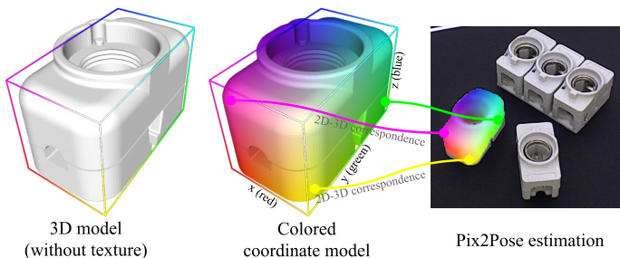
Figure 1. An example of converting a 3D model to a colored coordinate model. Normalized coordinates of each vertex are directly mapped to red, green and blue values in the color space. Pix2Pose predicts these colored images to build a 2D-3D correspondence per pixel directly without any feature matching operation.
图 1: 将3D模型转换为彩色坐标模型的示例。每个顶点的归一化坐标直接映射到色彩空间中的红、绿、蓝值。Pix2Pose通过预测这些彩色图像直接建立逐像素的2D-3D对应关系,无需任何特征匹配操作。
A large body of work relies on the textured 3D model of an object, which is made by a 3D scanning device, e.g., BigBIRD Object Scanning Rig [36], and provided by a dataset to render synthetic images for training [15, 29] or refinement [19, 22]. Thus, the quality of texture in the 3D model should be sufficient to render visually correct images. Unfortunately, this is not applicable to domains that do not have textured 3D models such as industry that commonly use texture-less CAD models. Since the texture quality of a reconstructed 3D model varies with method, camera, and camera trajectory during the reconstruction process, it is difficult to guarantee sufficient quality for training. Therefore, it is beneficial to predict poses without textures on 3D models to achieve more robust estimation regardless of the texture quality.
大量研究工作依赖于物体的带纹理3D模型,这些模型通常由3D扫描设备(如BigBIRD物体扫描装置[36])制作,并通过数据集提供以渲染合成图像用于训练[15,29]或优化[19,22]。因此,3D模型中的纹理质量必须足以渲染出视觉正确的图像。遗憾的是,这种方法不适用于缺乏带纹理3D模型的领域,例如普遍使用无纹理CAD模型的工业领域。由于重建3D模型的纹理质量会随重建过程中采用的方法、相机及相机轨迹而变化,很难保证训练所需的纹理质量。因此,在3D模型上实现无纹理的姿态预测,将有助于获得不受纹理质量影响的更鲁棒估计结果。
Even though recent studies have shown great potential to estimate pose without textured 3D models using Convolutional Neural Networks (CNN) [2, 4, 25, 30], a significant challenge is to estimate correct poses when objects are occluded or symmetric. Training CNNs is often distracted by symmetric poses that have similar appearance inducing very large errors in a naive loss function. In previous work, a strategy to deal with symmetric objects is to limit the range of poses while rendering images for training [15, 23] or simply to apply a transformation from the pose outside of the limited range to a symmetric pose within the range [25] for real images with pose annotations. This approach is sufficient for objects that have infinite and continuous symmetric poses on a single axis, such as cylinders, by simply ignoring the rotation about the axis. However, as pointed in [25], when an object has a finite number of symmetric poses, it is difficult to determine poses around the boundaries of view limits. For example, if a box has an angle of symmetry, $\pi$ , with respect to an axis and a view limit between 0 and $\pi$ , the pose at $\pi+\alpha(\alpha\approx0,\alpha>0)$ has to be transformed to a symmetric pose at $\alpha$ even if the detailed appearance is closer to a pose at $\pi$ . Thus, a loss function has to be investigated to guide pose estimations to the closest symmetric pose instead of explicitly defined view ranges.
尽管近期研究表明,利用卷积神经网络 (CNN) [2, 4, 25, 30] 无需纹理3D模型即可估计姿态具有巨大潜力,但在物体被遮挡或对称时正确估计姿态仍面临重大挑战。训练CNN时,对称姿态的相似外观容易干扰模型,导致朴素损失函数产生极大误差。先前工作中,处理对称物体的策略包括:在渲染训练图像时限制姿态范围 [15, 23],或对带有姿态标注的真实图像,直接将超出限定范围的姿态转换至范围内的对称姿态 [25]。这种方法对于单轴无限连续对称的物体(如圆柱体)已足够——只需忽略绕该轴的旋转。但如[25]所述,当物体具有有限数量对称姿态时,视图边界附近的姿态难以确定。例如,若盒子相对于某轴的对称角度为$\pi$,且视图限制在0到$\pi$之间,则位于$\pi+\alpha(\alpha\approx0,\alpha>0)$的姿态必须转换至$\alpha$处的对称姿态,即使其细节外观更接近$\pi$处的姿态。因此,需要研究能引导姿态估计指向最近对称姿态的损失函数,而非依赖显式定义的视图范围。
This paper proposes a novel method, Pix2Pose, that can supplement any 2D detection pipeline for additional pose estimation. Pix2Pose predicts pixel-wise 3D coordinates of an object using RGB images without textured 3D models for training. The 3D coordinates of occluded pixels are implicitly estimated by the network in order to be robust to occlusion. A specialized loss function, the transformer loss, is proposed to robustly train the network with symmetric objects. As a result of the prediction, each pixel forms a 2D-3D correspondence that is used to compute poses by the Perspective-n-Point algorithm $(\mathrm{PnP})$ [18].
本文提出了一种名为Pix2Pose的新方法,能够为任何2D检测流程补充姿态估计功能。Pix2Pose通过RGB图像预测物体的逐像素3D坐标,且无需纹理化3D模型进行训练。该网络通过隐式估算被遮挡像素的3D坐标,从而实现对遮挡的鲁棒性。针对对称物体,我们提出了一种专用损失函数——transformer loss (变换器损失) 来鲁棒地训练网络。预测结果中每个像素都会形成2D-3D对应关系,通过Perspective-n-Point算法 (PnP) [18] 计算姿态。
To summarize, the contributions of the paper are: (1) A novel framework for 6D pose estimation, Pix2Pose, that robustly regresses pixel-wise 3D coordinates of objects from RGB images using 3D models without textures during training. (2) A novel loss function, the transformer loss, for handling symmetric objects that have a finite number of ambiguous views. (3) Experimental results on three different datasets, LineMOD [9], LineMOD Occlusion [1], and TLess [10], showing that Pix2Pose outperforms the state-ofthe-art methods even if objects are occluded or symmetric.
综上所述,本文的贡献在于:(1) 提出了一种新颖的6D姿态估计框架Pix2Pose,该框架在训练阶段仅使用无纹理的3D模型,即可从RGB图像中稳健地回归出物体逐像素的3D坐标。(2) 针对具有有限数量模糊视角的对称物体,提出了一种新型损失函数——transformer loss。(3) 在LineMOD [9]、LineMOD Occlusion [1]和TLess [10]三个不同数据集上的实验结果表明,即使物体存在遮挡或对称性,Pix2Pose仍能超越现有最优方法。
The remainder of this paper is organized as follows. A brief summary of related work is provided in Sec. 2. Details of Pix2Pose and the pose prediction process are explained in Sec. 3 and Sec. 4. Experimental results are reported in Sec. 5 to compare our approach with the state-of-the-art methods. The paper concludes in Sec. 6.
本文的其余部分组织如下。第2节简要概述了相关工作。第3节和第4节详细解释了Pix2Pose及位姿预测过程。第5节报告了实验结果,将我们的方法与最先进方法进行了比较。第6节对全文进行了总结。
2. Related work
2. 相关工作
This section gives a brief summary of previous work related to pose estimation using RGB images. Three different approaches for pose estimation using CNNs are discussed and the recent advances of generative models are reviewed.
本节简要概述了与基于RGB图像的姿态估计相关的前期工作,讨论了使用CNN进行姿态估计的三种不同方法,并回顾了生成式模型的最新进展。
CNN based pose estimation The first, and simplest, method to estimate the pose of an object using a CNN is to predict a representation of a pose directly such as the locations of projected points of 3D bounding boxes [25, 30], classified view points [15], unit qua tern ions and translations [33], or the Lie algebra representation, $s o(3)$ , with the translation of $z$ -axis [4]. Except for methods that predict projected points of the 3D bounding box, which requires further computations for the $\mathrm{PnP}$ algorithm, the direct regression is computationally efficient since it does not require additional computation for the pose. The drawback of these methods, however, is the lack of correspondences that can be useful to generate multiple pose hypotheses for the robust estimation of occluded objects. Furthermore, symmetric objects are usually handled by limiting the range of viewpoints, which sometimes requires additional treatments, e.g., training a CNN for classifying view ranges [25]. Xiang et al. [33] propose a loss function that computes the average distance to the nearest points of transformed models in an estimated pose and an annotated pose. However, searching for the nearest 3D points is time consuming and makes the training process inefficient.
基于CNN的姿态估计
第一种也是最简单的方法是使用CNN直接预测姿态的表示,例如3D边界框投影点的位置[25, 30]、分类视点[15]、单位四元数与平移量[33],或李代数表示 $s o(3)$ 与 $z$ 轴平移量[4]。除了预测3D边界框投影点的方法需要为PnP算法进行额外计算外,直接回归在计算上效率较高,因为它不需要为姿态进行额外计算。然而,这些方法的缺点在于缺乏可用于生成多个姿态假设的对应关系,这对于被遮挡物体的鲁棒估计很有用。此外,对称物体通常通过限制视点范围来处理,这有时需要额外处理,例如训练CNN对视点范围进行分类[25]。Xiang等人[33]提出了一种损失函数,计算在估计姿态和标注姿态下变换模型最近点的平均距离。然而,搜索最近的3D点非常耗时,导致训练过程效率低下。
The second method is to match features to find the nearest pose template and use the pose information of the template as an initial guess [9]. Recently, S under meyer et al. [29] propose an auto-encoder network to train implicit representations of poses without supervision using RGB images only. Manual handling of symmetric objects is not necessary for this work since the implicit representation can be close to any symmetric view. However, it is difficult to specify 3D translations using rendered templates that only give a good estimation of rotations. The size of the 2D bounding box is used to compute the $z$ -component of 3D translation, which is too sensitive to small errors of 2D bounding boxes that are given from a 2D detection method.
第二种方法是通过特征匹配找到最近的姿态模板,并使用该模板的姿态信息作为初始猜测 [9]。最近,Sundermeyer等人 [29] 提出了一种自编码器网络,仅使用RGB图像无监督地训练姿态的隐式表示。由于隐式表示可以接近任何对称视角,因此这项工作无需手动处理对称物体。然而,仅通过渲染模板(这些模板能较好估计旋转)难以精确指定3D平移。2D边界框的尺寸被用于计算3D平移的$z$分量,但该方法对2D检测方法给出的边界框小误差过于敏感。
The last method is to predict 3D locations of pixels or local shapes in the object space [2, 16, 23]. Brachmann et al. [2] regress 3D coordinates and predict a class for each pixel using the auto-context random forest. Oberwerger et al. [23] predict multiple heat-maps to localize the 2D projections of 3D points of objects using local patches. These methods are robust to occlusion because they focus on local information only. However, additional computation is required to derive the best result among pose hypotheses, which makes these methods slow.
最后一种方法是预测物体空间中像素或局部形状的3D位置 [2, 16, 23]。Brachmann等人 [2] 使用自动上下文随机森林回归3D坐标并为每个像素预测类别。Oberwerger等人 [23] 通过局部块预测多个热力图来定位物体3D点的2D投影。这些方法对遮挡具有鲁棒性,因为它们仅关注局部信息。然而,需要在位姿假设中通过额外计算得出最佳结果,这使得这些方法速度较慢。
The method proposed in this paper belongs to the last category that predicts 3D locations of pixels in the object frame as in [1, 2]. Instead of detecting an object using local patches from sliding windows, an independent 2D detection network is employed to provide areas of interest for target objects as performed in [29].
本文提出的方法属于最后一类,即如[1, 2]所述预测像素在物体坐标系中的3D位置。与通过滑动窗口的局部块检测物体不同,如[29]所述,该方法采用独立的2D检测网络来提供目标物体的感兴趣区域。
Generative models Generative models using autoencoders have been used to de-noise [32] or recover the missing parts of images [34]. Recently, using Generative Adversarial Network (GAN) [6] improves the quality of generated images that are less blurry and more realistic, which are used for the image-to-image translation [14], image in-painting and de-noising [12, 24] tasks. Zakharov et al. [35] propose a GAN based framework to convert a real depth image to a synthetic depth image without noise and background for classification and pose estimation.
生成模型
使用自动编码器 (autoencoders) 的生成模型已被用于去噪 [32] 或恢复图像的缺失部分 [34]。近年来,生成对抗网络 (GAN) [6] 的运用提升了生成图像的质量,使其更清晰、更逼真,这些技术被应用于图像到图像转换 [14]、图像修复和去噪 [12, 24] 等任务。Zakharov 等人 [35] 提出了一种基于 GAN 的框架,将真实深度图像转换为无噪声和背景的合成深度图像,用于分类和姿态估计。
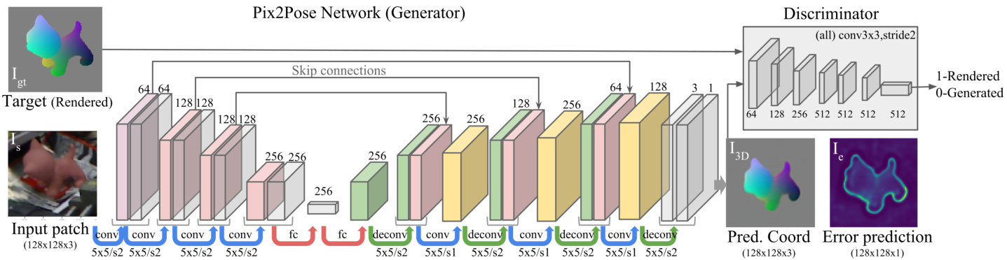
Figure 2. An overview of the architecture of Pix2Pose and the training pipeline.
图 2: Pix2Pose架构及训练流程概览。
Inspired by previous work, we train an auto-encoder architecture with GAN to convert color images to coordinate values accurately as in the image-to-image translation task while recovering values of occluded parts as in the image in-painting task.
受前人工作启发,我们采用带GAN的自动编码器架构进行训练,在实现图像到图像翻译任务精准转换彩色图像为坐标值的同时,还能像图像修复任务那样还原被遮挡部分的数据值。
3. Pix2Pose
3. Pix2Pose
This section provides a detailed description of the network architecture of Pix2Pose and loss functions for training. As shown in Fig. 2, Pix2Pose predicts 3D coordinates of individual pixels using a cropped region containing an object. The robust estimation is established by recovering 3D coordinates of occluded parts and using all pixels of an object for pose prediction. A single network is trained and used for each object class. The texture of a 3D model is not necessary for training and inference.
本节详细介绍了Pix2Pose的网络架构和训练所用的损失函数。如图2所示,Pix2Pose通过包含物体的裁剪区域来预测单个像素的3D坐标。该方法通过恢复被遮挡部分的3D坐标,并利用物体的所有像素进行位姿预测,从而建立鲁棒估计。每个物体类别都单独训练并使用一个网络。训练和推理过程中无需使用3D模型的纹理信息。
3.1. Network Architecture
3.1. 网络架构
The architecture of the Pix2Pose network is described in Fig. 2. The input of the network is a cropped image $I_{\mathrm{s}}$ using a bounding box of a detected object class. The outputs of the network are normalized 3D coordinates of each pixel ${I_{\mathrm{3D}}}$ in the object coordinate and estimated errors $I_{\mathrm{e}}$ of each prediction, $I_{3\mathrm{D}},I_{\mathrm{e}}=G(I_{\mathrm{s}})$ , where $G$ denotes the Pix2Pose network. The target output includes coordinate predictions of occluded parts, which makes the prediction more robust to partial occlusion. Since a coordinate consists of three values similar to RGB values in an image, the output ${I_{\mathrm{3D}}}$ can be regarded as a color image. Therefore, the ground truth output is easily derived by rendering the colored coordinate model in the ground truth pose. An example of 3D coordinate values in a color image is visualized in Fig. 1. The error prediction $I_{e}$ is regarded as a confidence score of each pixel, which is directly used to determine outlier and inlier pixels before the pose computation.
Pix2Pose网络架构如图2所示。网络输入是通过检测到的物体类别边界框裁剪后的图像$I_{\mathrm{s}}$。网络输出为物体坐标系中每个像素的归一化3D坐标${I_{\mathrm{3D}}}$以及每个预测的估计误差$I_{\mathrm{e}}$,即$I_{3\mathrm{D}},I_{\mathrm{e}}=G(I_{\mathrm{s}})$,其中$G$表示Pix2Pose网络。目标输出包含被遮挡部分的坐标预测,这使得预测对部分遮挡更具鲁棒性。由于坐标由三个值组成(类似于图像中的RGB值),输出${I_{\mathrm{3D}}}$可视为彩色图像。因此,通过在地面真实姿态下渲染彩色坐标模型,可以轻松获得真实输出。图1展示了彩色图像中3D坐标值的可视化示例。误差预测$I_{e}$被视为每个像素的置信度分数,在姿态计算前直接用于判定离群点和内点像素。
The cropped image patch is resized to $128\times128p x$ with three channels for RGB values. The sizes of filters and channels in the first four convolutional layers, the encoder, are the same as in [29]. To maintain details of low-level feature maps, skip connections [28] are added by copying the half channels of outputs from the first three layers to the corresponding symmetric layers in the decoder, which results in more precise estimation of pixels around geometrical boundaries. The filter size of every convolution and de convolution layer is fixed to $5\times5$ with stride 1 or 2 denoted as $s l$ or $s2$ in Fig. 2. Two fully connected layers are applied for the bottle neck with 256 dimensions between the encoder and the decoder. The batch normalization [13] and the LeakyReLU activation are applied to every output of the intermediate layers except the last layer. In the last layer, an output with three channels and the tanh activation produces a 3D coordinate image ${I_{\mathrm{3D}}}$ , and another output with one channel and the sigmoid activation estimates the expected errors $I_{\mathrm{e}}$ .
裁剪后的图像块被调整为$128\times128p x$,包含RGB三通道。前四个卷积层(编码器)的滤波器尺寸和通道数与[29]相同。为保留低级特征图的细节,通过将前三层输出的半数通道复制到解码器中对应的对称层,添加了跳跃连接[28],从而更精确地估计几何边界周围的像素。每个卷积层和反卷积层的滤波器尺寸固定为$5\times5$,步长为1或2(在图2中分别标记为$s l$或$s2$)。编码器与解码器之间采用两个全连接层作为256维瓶颈结构。除最后一层外,所有中间层输出均应用批量归一化[13]和LeakyReLU激活函数。最后一层中,采用tanh激活的三通道输出生成3D坐标图像${I_{\mathrm{3D}}}$,另一单通道输出通过sigmoid激活函数估计预期误差$I_{\mathrm{e}}$。
3.2. Network Training
3.2. 网络训练
The main objective of training is to predict an output that minimizes errors between a target coordinate image and a predicted image while estimating expected errors of each pixel.
训练的主要目标是在预测输出时,最小化目标坐标图像与预测图像之间的误差,同时估计每个像素的预期误差。
Transformer loss for 3D coordinate regression To reconstruct the desired target image, the average L1 distance of each pixel is used. Since pixels belonging to an object are more important than the background, the errors under the object mask are multiplied by a factor of $\beta$ $(\geq1)$ to weight errors in the object mask. The basic reconstruction loss $\mathscr{L}_{\mathrm{r}}$ is defined as,
3D坐标回归的Transformer损失
为了重建目标图像,使用每个像素的平均L1距离。由于属于物体的像素比背景更重要,物体掩膜下的误差会乘以系数$\beta$ $(\geq1)$来加权。基础重建损失$\mathscr{L}_{\mathrm{r}}$定义为:
$$
\mathcal{L}{\mathrm{r}}=\frac{1}{n}\Big[\beta\sum_{i\in M}||I_{3\mathrm{D}}^{i}-I_{\mathrm{gt}}^{i}||{1}+\sum_{i\notin M}||I_{3\mathrm{D}}^{i}-I_{\mathrm{gt}}^{i}||_{1}\Big],
$$
$$
\mathcal{L}{\mathrm{r}}=\frac{1}{n}\Big[\beta\sum_{i\in M}||I_{3\mathrm{D}}^{i}-I_{\mathrm{gt}}^{i}||{1}+\sum_{i\notin M}||I_{3\mathrm{D}}^{i}-I_{\mathrm{gt}}^{i}||_{1}\Big],
$$
where $n$ is the number of pixels, $I_{\mathrm{gt}}^{i}$ is the $i^{\mathrm{th}}$ pixel of the target image, and $M$ denotes an object mask of the target image, which includes pixels belonging to the object when it is fully visible. Therefore, this mask also contains the occluded parts to predict the values of invisible parts for robust estimation of occluded objects.
其中 $n$ 是像素数量,$I_{\mathrm{gt}}^{i}$ 是目标图像的第 $i$ 个像素,$M$ 表示目标图像的对象掩码 (object mask)。该掩码包含物体完全可见时所属的像素,因此也涵盖被遮挡部分,以便预测不可见区域的值从而实现遮挡物体的鲁棒性估计。
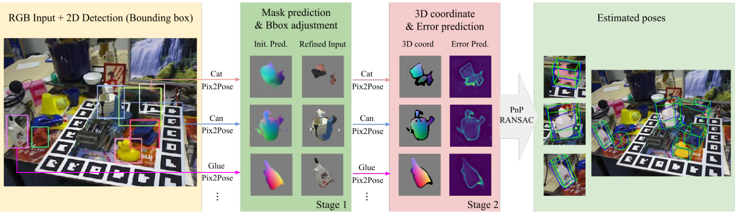
Figure 3. An example of the pose estimation process. An image and 2D detection results are the input. In the first stage, the predicted results are used to specify important pixels and adjust bounding boxes while removing backgrounds and uncertain pixels. In the second stage, pixels with valid coordinate values and small error predictions are used to estimate poses using the PnP algorithm with RANSAC. Green and blue lines in the result represent 3D bounding boxes of objects in ground truth poses and estimated poses.
图 3: 姿态估计流程示例。输入为图像和 2D 检测结果。第一阶段使用预测结果标记重要像素并调整边界框,同时移除背景和不确定像素。第二阶段利用具有有效坐标值和小误差预测的像素,通过 RANSAC 的 PnP 算法进行姿态估计。结果中的绿色和蓝色线条分别表示真实姿态和估计姿态下物体的 3D 边界框。
The loss above cannot handle symmetric objects since it penalizes pixels that have larger distances in the 3D space without any knowledge of the symmetry. Having the advantage of predicting pixel-wise coordinates, the 3D coordinate of each pixel is easily transformed to a symmetric pose by multiplying a 3D transformation matrix to the target image directly. Hence, the loss can be calculated for a pose that has the smallest error among symmetric pose candidates as formulated by,
上述损失函数无法处理对称物体,因为它会在不了解对称性的情况下惩罚3D空间中距离较远的像素。得益于逐像素坐标预测的优势,通过直接将3D变换矩阵作用于目标图像,即可轻松将每个像素的3D坐标转换为对称姿态。因此,可按以下公式计算对称候选姿态中误差最小的姿态对应的损失值:
$$
\mathcal{L}{3\mathrm{D}}=\operatorname*{min}{p\in\mathrm{sym}}\mathcal{L}{\mathrm{r}}(I_{3\mathrm{D}},R_{p}I_{g t}),
$$
$$
\mathcal{L}{3\mathrm{D}}=\operatorname*{min}{p\in\mathrm{sym}}\mathcal{L}{\mathrm{r}}(I_{3\mathrm{D}},R_{p}I_{g t}),
$$
where $R_{p}\in\mathbb{R}^{3\mathrm{x3}}$ is a transformation from a pose to a symmetric pose in a pool of symmetric poses, sym, including an identity matrix for the given pose. The pool sym is assumed to be defined before the training of an object. This novel loss, the transformer loss, is applicable to any symmetric object that has a finite number of symmetric poses. This loss adds only a tiny effort for computation since a small number of matrix multiplications is required. The transformer loss in Eq. 2 is applied instead of the basic reconstruction loss in Eq. 1. The benefit of the transformer loss is analyzed in Sec. 5.7.
其中 $R_{p}\in\mathbb{R}^{3\mathrm{x3}}$ 是从姿态到对称姿态池 sym 中某个对称姿态的变换矩阵,该池包含给定姿态的单位矩阵。假设对称池 sym 在物体训练前就已定义好。这种新颖的损失函数——变换器损失 (transformer loss) 适用于任何具有有限对称姿态的对称物体。由于只需少量矩阵乘法运算,该损失仅增加极小的计算开销。式2中的变换器损失将替代式1中的基础重构损失。第5.7节将分析变换器损失的优势。
Loss for error prediction The error prediction $I_{e}$ estimates the difference between the predicted image ${I_{\mathrm{3D}}}$ and the target image $I_{\mathrm{gt}}$ . This is identical to the reconstruction loss $\mathcal{L}{\mathrm{r}}$ with $\beta=1$ such that pixels under the object mask are not penalized. Thus, the error prediction loss $\mathcal{L}_{\mathrm{e}}$ is written as,
误差预测损失 误差预测 $I_{e}$ 用于估计预测图像 ${I_{\mathrm{3D}}}$ 与目标图像 $I_{\mathrm{gt}}$ 之间的差异。这与重建损失 $\mathcal{L}{\mathrm{r}}$ 相同(当 $\beta=1$ 时),使得物体掩膜下的像素不受惩罚。因此,误差预测损失 $\mathcal{L}_{\mathrm{e}}$ 可表示为:
$$
\mathcal{L}{\mathrm{e}}=\frac{1}{n}\sum_{i}||I_{\mathrm{e}}^{i}-\operatorname*{min}[\mathcal{L}{\mathrm{r}}^{i},1]||_{2}^{2},\beta=1.
$$
$$
\mathcal{L}{\mathrm{e}}=\frac{1}{n}\sum_{i}||I_{\mathrm{e}}^{i}-\operatorname*{min}[\mathcal{L}{\mathrm{r}}^{i},1]||_{2}^{2},\beta=1.
$$
The error is bounded to the maximum value of the sigmoid function.
误差受限于sigmoid函数的最大值。
Traininig with GAN As discussed in Sec. 2, the network training with GAN generates more precise and realistic images in a target domain using images of another domain [14]. The task for Pix2Pose is similar to this task since it converts a color image to a 3D coordinate image of an object. Therefore, the disc rim in at or and the loss function of GAN [6], $\mathcal{L}_{\mathrm{GAN}}$ , is employed to train the network. As shown in Fig. 2, the disc rim in at or network attempts to distinguish whether the 3D coordinate image is rendered by a 3D model or is estimated. The loss is defined as,
使用GAN进行训练
如第2节所述,使用GAN进行网络训练能通过另一域的图像生成目标域中更精确逼真的图像[14]。Pix2Pose的任务与此类似,因为它将彩色图像转换为物体的3D坐标图像。因此,我们采用GAN的判别器(discriminator)和损失函数[6] $\mathcal{L}_{\mathrm{GAN}}$ 来训练网络。如图2所示,判别器网络试图区分3D坐标图像是由3D模型渲染的还是估算得到的。该损失定义为:
$$
\begin{array}{r}{\mathcal{L}{\mathrm{GAN}}=\log D(I_{g t})+\log(1-D(G(I_{\mathrm{src}}))),}\end{array}
$$
$$
\begin{array}{r}{\mathcal{L}{\mathrm{GAN}}=\log D(I_{g t})+\log(1-D(G(I_{\mathrm{src}}))),}\end{array}
$$
where $\mathrm{D}$ denotes the disc rim in at or network. Finally, the objective of the training with GAN is formulated as,
其中 $\mathrm{D}$ 表示判别器 (discriminator) 网络。最终,生成对抗网络 (GAN) 的训练目标可表述为:
$$
\begin{array}{r}{G^{}=\arg\underset{G}{\operatorname*{min}}\underset{D}{\operatorname*{max}}\mathcal{L}{\mathrm{GAN}}(G,D)+\lambda_{1}\mathcal{L}{3\mathrm{D}}(G)+\lambda_{2}\mathcal{L}_{\mathrm{e}}(G),}\end{array}
$$
$$
\begin{array}{r}{G^{}=\arg\underset{G}{\operatorname*{min}}\underset{D}{\operatorname*{max}}\mathcal{L}{\mathrm{GAN}}(G,D)+\lambda_{1}\mathcal{L}{3\mathrm{D}}(G)+\lambda_{2}\mathcal{L}_{\mathrm{e}}(G),}\end{array}
$$
where $\lambda_{1}$ and $\lambda_{2}$ denote weights to balance different tasks.
其中 $\lambda_{1}$ 和 $\lambda_{2}$ 表示用于平衡不同任务的权重。
4. Pose prediction
4. 姿态预测
This section gives a description of the process that computes a pose using the output of the Pix2Pose network. The overview of the process is shown in Fig. 3. Before the estimation, the center, width, and height of each bounding box are used to crop the region of interest and resize it to the input size, $128\times128p x$ . The width and height of the region are set to the same size to keep the aspect ratio by taking the larger value. Then, they are multiplied by a factor of 1.5 so that the cropped region potentially includes occluded parts. The pose prediction is performed in two stages and the identical network is used in both stages. The first stage aligns the input bounding box to the center of the object which could be shifted due to different 2D detection methods. It also removes unnecessary pixels (background and uncertain) that are not preferred by the network. The second stage predicts a final estimation using the refined input from the first stage and computes the final pose.
本节描述了利用Pix2Pose网络输出计算位姿的过程,整体流程如图3所示。在估计前,首先利用每个边界框的中心点、宽度和高度裁剪感兴趣区域,并将其缩放至$128\times128p x$的输入尺寸。为确保长宽比不变,区域的宽高取较大值设为相同尺寸,随后乘以1.5倍系数以使裁剪区域可能包含被遮挡部分。位姿预测分两个阶段执行,两阶段使用相同网络:第一阶段将可能因不同2D检测方法产生偏移的输入边界框对齐至物体中心,同时去除网络中不希望的冗余像素(背景及不确定区域);第二阶段利用第一阶段优化后的输入预测最终估计值并计算位姿。
Stage 1: Mask prediction and Bbox Adjustment In this stage, the predicted coordinate image ${I_{\mathrm{3D}}}$ is used for specifying pixels that belong to the object including the occluded parts by taking pixels with non-zero values. The error prediction is used to remove the uncertain pixels if an error for a pixel is larger than the outlier threshold $\theta_{o}$ . The valid object mask is computed by taking the union of pixels that have non-zero values and pixels that have lower errors than $\theta_{o}$ . The new center of the bounding box is determined with the centroid of the valid mask. As a result, the output of the first stage is a refined input that only contains pixels in the valid mask cropped from a new bounding box. Examples of outputs of the first stage are shown in Fig. 3. The refined input possibly contains the occluded parts when the error prediction is below the outlier threshold $\theta_{o}$ , which means the coordinates of these pixels are easy to predict despite occlusions.
阶段1:掩码预测与边界框调整
在此阶段,利用预测的坐标图像 ${I_{\mathrm{3D}}}$ 通过选取非零值像素来指定属于目标物体(包括被遮挡部分)的像素。若某像素的误差超过离群阈值 $\theta_{o}$,则通过误差预测移除不确定像素。有效物体掩码通过取非零值像素与误差低于 $\theta_{o}$ 的像素的并集计算得出。边界框的新中心由有效掩码的质心确定。最终,第一阶段输出的是从新边界框裁剪出的、仅包含有效掩码内像素的优化输入。图3展示了该阶段的输出示例。当误差预测低于离群阈值 $\theta_{o}$ 时,优化输入可能包含被遮挡部分,这意味着尽管存在遮挡,这些像素的坐标仍易于预测。
Stage 2: Pixel-wise 3D coordinate regression with errors The second estimation with the network is performed to predict a coordinate image and expected error values using the refined input as depicted in Fig. 3. Black pixels in the 3D coordinate samples denote points that are removed when the error prediction is larger than the inlier threshold $\theta_{i}$ even though points have non-zero coordinate values. In other words, pixels that have non-zero coordinate values with smaller error predictions than $\theta_{i}$ are used to build 2D3D correspondences. Since each pixel already has a value for a 3D point in the object coordinate, the 2D image coordinates and predicted 3D coordinates directly form correspondences. Then, applying the $\mathrm{PnP}$ algorithm [18] with RANdom SAmple Consensus (RANSAC) [5] iteration computes the final pose by maximizing the number of inliers that have lower re-projection errors than a threshold $\theta_{r e}$ . It is worth mentioning that there is no rendering involved during the pose estimation since Pix2Pose does not assume textured 3D models. This also makes the estimation process fast.
阶段2:带误差的逐像素3D坐标回归
通过网络的第二次估计,使用优化后的输入预测坐标图像和预期误差值,如图3所示。3D坐标样本中的黑色像素表示即使该点具有非零坐标值,当误差预测大于内点阈值$\theta_{i}$时也会被移除的点。换句话说,仅保留误差预测小于$\theta_{i}$且具有非零坐标值的像素来建立2D-3D对应关系。由于每个像素已包含物体坐标系中的3D点值,2D图像坐标与预测的3D坐标直接形成对应关系。随后,应用$\mathrm{PnP}$算法[18]结合随机抽样一致(RANSAC)[5]迭代,通过最大化重投影误差低于阈值$\theta_{re}$的内点数量来计算最终位姿。值得注意的是,由于Pix2Pose不依赖带纹理的3D模型,位姿估计过程中无需渲染操作,这也使得估计过程更为快速。
5. Evaluation
5. 评估
In this section, experiments on three different datasets are performed to compare the performance of Pix2Pose to state-of-the-art methods. The evaluation using LineMOD [9] shows the performance for objects without occlusion in the single object scenario. For the multiple object scenario with occlusions, LineMOD Occlusion [1] and T-Less [10] are used. The evaluation on T-Less shows the most significant benefit of Pix2Pose since T-Less provides texture-less CAD models and most of the objects are symmetric, which is more challenging and common in industrial domains.
在本节中,我们在三个不同数据集上进行了实验,以比较Pix2Pose与最先进方法的性能。使用LineMOD [9]的评估展示了单物体场景下无遮挡物体的性能。对于存在遮挡的多物体场景,我们采用了LineMOD Occlusion [1]和T-Less [10]。在T-Less上的评估最能体现Pix2Pose的优势,因为T-Less提供了无纹理的CAD模型且大部分物体具有对称性,这在工业领域中更具挑战性和普遍性。
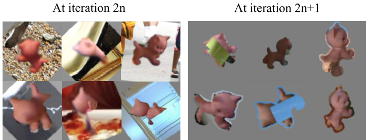
Figure 4. Examples of mini-batches for training. A mini-batch is altered for every training iteration. Left: images for the first stage, Right: images for the second stage.
图 4: 训练用的小批量(mini-batch)示例。每个训练迭代都会改变小批量的组成。左图: 第一阶段的图像,右图: 第二阶段的图像。
5.1. Augmentation of training data
5.1. 训练数据增强
A small number of real images are used for training with various augmentations. Image pixels of objects are extracted from real images and pasted to background images that are randomly picked from the Coco dataset [21]. After applying the color augmentations on the image, the borderlines between the object and the background are blurred to make smooth boundaries. A part of the object area is replaced by the background image to simulate occlusion. Lastly, a random rotation is applied to both the augmented color image and the target coordinate image. The same augmentation is applied to all evaluations except sizes of occluded areas that need to be larger for datasets with occlusions, LineMOD Occlusion and T-Less. Sample augmentated images are shown in Fig. 4. As explained in Sec. 4, the network recognizes two types of inputs, with background in the first stage and without background pixels in the second stage. Thus, a mini-batch is altered for every iteration as shown in Fig. 4. Target coordinate images are rendered before training by placing the object in the ground truth poses using the colored coordinate model as in Fig. 1.
训练时使用少量真实图像并进行多种增强处理。从真实图像中提取物体的像素,并将其粘贴到从Coco数据集[21]随机选取的背景图像上。对图像进行色彩增强后,模糊物体与背景之间的边界线以实现平滑过渡。用背景图像替换部分物体区域以模拟遮挡效果。最后,对增强后的彩色图像和目标坐标图像同时施加随机旋转。除遮挡区域大小需针对含遮挡的数据集(LineMOD Occlusion和T-Less)增大外,所有评估均采用相同增强方式。增强样本示例如图4所示。如第4节所述,网络分两阶段识别输入:第一阶段包含背景像素,第二阶段不含背景像素。因此,每次迭代都会按图4所示调整小批量数据。目标坐标图像通过将物体置于真实位姿(使用图1的彩色坐标模型)在训练前渲染生成。
5.2. Implementation details
5.2. 实现细节
For training, the batch size of each iteration is set to 50, the Adam optimizer [17] is used with initial learning rate of 0.0001 for 25K iterations. The learning rate is multiplied by a factor of 0.1 for every 12K iterations. Weights of loss functions in Eq. 1 and Eq. 5 are: $\beta{=}3$ , $\lambda_{1}{=}100$ and $\lambda_{\mathrm{2}}\mathbf{=}50$ . For evaluation, a 2D detection network and Pix2Pose networks of all object candidates in test sequences are loaded to the GPU memory, which requires approximately 2.2GB for the LineMOD Occlusion experiment with eight objects. The standard parameters for the inference are: $\theta_{i}{=}0.1$ , $\theta_{o}{=}[0.1,0.2,0.3]$ , and $\theta_{r e}{=}3$ . Since the values of error predictions are biased by the level of occlusion in the online augmentation and the shape and size of each object, the outlier threshold $\theta_{o}$ in the first stage is determined among three values to include more numbers of visible pixels while excluding noisy pixels using samples of training images with artificial occlusions. More details about parameters are given in the supplementary material. The training and evaluations are performed with an Nvidia GTX 1080 GPU and i7-6700K CPU.
训练时,每次迭代的批量大小(batch size)设为50,使用Adam优化器[17],初始学习率为0.0001进行25K次迭代。每12K次迭代后学习率乘以0.1的衰减系数。公式1和公式5中损失函数的权重分别为:$\beta{=}3$、$\lambda_{1}{=}100$和$\lambda_{\mathrm{2}}\mathbf{=}50$。评估时,测试序列中所有候选物体的2D检测网络和Pix2Pose网络会被加载到GPU显存中,在包含8个物体的LineMOD遮挡实验中约需2.2GB显存。标准推理参数为:$\theta_{i}{=}0.1$、$\theta_{o}{=}[0.1,0.2,0.3]$以及$\theta_{r e}{=}3$。由于在线数据增强中误差预测值受遮挡程度及各物体形状尺寸的影响,第一阶段离群值阈值$\theta_{o}$从三个候选值中选定,旨在通过人工遮挡的训练图像样本,在排除噪声像素的同时纳入更多可见像素。更多参数细节见补充材料。训练与评估使用Nvidia GTX 1080 GPU和i7-6700K CPU完成。
| ape | bvise | cam | can | cat | driller | duck | e.box* | glue* | holep | iron | lamp | phone | avg | |
|---|---|---|---|---|---|---|---|---|---|---|---|---|---|---|
| Pix2Pose | 58.1 | 91.0 | 60.9 | 84.4 | 65.0 | 76.3 | 43.8 | 96.8 | 79.4 | 74.8 | 83.4 | 82.0 | 45.0 | 72.4 |
| Tekin [30] | 21.6 | 81.8 | 36.6 | 68.8 | 41.8 | 63.5 | 27.2 | 69.6 | 80.0 | 42.6 | 75.0 | 71.1 | 47.7 | 56.0 |
| Brachmann [2] | 33.2 | 64.8 | 38.4 | 62.9 | 42.7 | 61.9 | 30.2 | 49.9 | 31.2 | 52.8 | 80.0 | 67.0 | 38.1 | 50.2 |
| BB8 [25] | 27.9 | 62.0 | 40.1 | 48.1 | 45.2 | 58.6 | 32.8 | 40.0 | 27.0 | 42.4 | 67.0 | 39.9 | 35.2 | 43.6 |
| Lienet30% [4] | 38.8 | 71.2 | 52.5 | 86.1 | 66.2 | 82.3 | 32.5 | 79.4 | 63.7 | 56.4 | 65.1 | 89.4 | 65.0 | 65.2 |
| BB8ref [25] | 40.4 | 91.8 | 55.7 | 64.1 | 62.6 | 74.4 | 44.3 | 57.8 | 41.2 | 67.2 | 84.7 | 76.5 | 54.0 | 62.7 |
| Implicitsyn [29] | 4.0 | 20.9 | 30.5 | 35.9 | 17.9 | 24.0 | 4.9 | 81.0 | 45.5 | 17.6 | 32.0 | 60.5 | 33.8 | 31.4 |
| SSD-6Dsyn/ref [15] | 65 | 80 | 78 | 86 | 70 | 73 | 66 | 100 | 100 | 49 | 78 | 73 | 79 | 76.7 |
| Radsyn/ref [26] | - | - | - | - | - | - | - | 78.7 |
2D detection network An improved Faster R-CNN [7, 27] with Resnet-101 [8] and Retinanet [20] with Resnet50 are employed to provide classes of detected objects with 2D bounding boxes for all target objects of each evaluation. The networks are initialized with pre-trained weights using the Coco dataset [21]. The same set of real training images is used to generate training images. Cropped patches of objects in real images are pasted to random background images to generate training images that contain multiple classes in each image.
2D检测网络 采用改进的Faster R-CNN [7, 27](基于Resnet-101 [8])和Retinanet [20](基于Resnet50)为每次评估的所有目标对象提供带2D边界框的检测类别。网络使用Coco数据集 [21] 的预训练权重进行初始化。同一组真实训练图像被用于生成训练图像,通过将真实图像中物体的裁剪块粘贴到随机背景图像上,生成每张图像包含多个类别的训练数据。
5.3. Metrics
5.3. 指标
A standard metric for LineMOD, $\mathrm{AD}{\mathrm{D}|\mathrm{I}}$ , is mainly used for the evaluation [9]. This measures the average distance of vertices between a ground truth pose and an estimated pose. For symmetric objects, the average distance to the nearest vertices is used instead. The pose is considered correct when the error is less than $10%$ of the maximum 3D diameter of an object.
LineMOD的标准度量指标 $\mathrm{AD}{\mathrm{D}|\mathrm{I}}$ 主要用于评估[9]。该指标计算真实姿态与估计姿态之间顶点平均距离。对于对称物体,则改用最近顶点平均距离。当误差小于物体最大3D直径的 $10%$ 时,认为姿态估计正确。
For T-Less, the Visible Surface Discrepancy (VSD) is used as a metric since the metric is employed to benchmark various 6D pose estimation methods in [11]. This metric measures distance errors of visible parts only, which makes the metric invariant to ambiguities caused by symmetries and occlusion. As in previous work, the pose is regarded as correct when the error is less than 0.3 with $\tau{=}20m m$ and $\delta{=}15m m$ .
对于T-Less数据集,采用可见表面差异(VSD)作为评估指标,因为该指标在[11]中被用于基准测试多种6D姿态估计方法。该指标仅测量可见部分的距离误差,使其对对称性和遮挡引起的模糊性具有不变性。如先前工作所述,当误差小于0.3($\tau{=}20mm$ 和 $\delta{=}15mm$)时,姿态被视为正确。
5.4. LineMOD
5.4. LineMOD
For training, test sequences are separated into a training and test set. The divided set of each sequence is identical to the work of [2, 30], which uses $15%$ of test scenes, approximate ly less than 200 images per object, for training. A detection result, using Faster R-CNN, of an object with the highest score in each scene is used for pose estimation since the detection network produces multiple results for all 13 objects. For the symmetric objects, marked with $({}^{*})$ in Table 1, the pool of symmetric poses sym is defined as, $s y m=[I,R_{z}^{\pi}]$ , where $R_{z}^{\pi}$ represents a transformation matrix of rotation with $\pi$ about the $z$ -axis.
训练时,测试序列被分为训练集和测试集。每个序列的划分方式与[2, 30]的研究相同,即使用$15%$的测试场景(每个物体约少于200张图像)进行训练。由于检测网络会对所有13个物体生成多个检测结果,因此选用Faster R-CNN在每场景中对得分最高的物体检测结果进行位姿估计。对于表1中标有$({}^{*})$的对称物体,其对称位姿池sym定义为$sym=[I,R_{z}^{\pi}]$,其中$R_{z}^{\pi}$表示绕$z$轴旋转$\pi$的变换矩阵。
Table 2. LineMOD Occlusion: object recall $(\mathrm{AD{D|I}}{-}10%)$ . $(^{\dagger})$ indicates the method uses synthetically rendered images and real images for training, which has better coverage of viewpoints.
表 2. LineMOD遮挡场景下的物体召回率 $(\mathrm{AD{D|I}}{-}10%)$。$(^{\dagger})$表示该方法使用合成渲染图像和真实图像进行训练,具有更好的视角覆盖范围。
| Method | Pix2Pose | Oberwegert [23] | PoseCNNt [33] | Tekin [30] |
|---|---|---|---|---|
| ape can cat | 22.0 44.7 22.7 | 17.6 53.9 3.31 | 9.6 45.2 0.93 | 2.48 17.48 0.67 |
| driller duck | 44.7 15.0 | 62.4 19.2 | 41.4 19.6 | 7.66 1.14 |
| eggbox* | 25.2 | 25.9 | 22.0 | |
| glue* holep | 32.4 49.5 | 39.6 21.3 | 38.5 22.1 | 10.08 5.45 |
The upper part of Table 1 shows Pix2Pose significantly outperforms state-of-the-art methods that use the same amount of real training images without textured 3D models. Even though methods on the bottom of Table 1 use a larger portion of training images, use textured 3D models for training or pose refinement, our method shows competitive results against these methods. The results on symmetric objects show the best performance among methods that do not perform pose refinement. This verifies the benefit of the transformer loss, which improves the robustness of initial pose predictions for symmetric objects.
表 1 上半部分显示,Pix2Pose 在使用相同数量真实训练图像且无纹理 3D 模型的情况下,显著优于现有最优方法。尽管表 1 底部列出的方法使用了更多训练图像、采用带纹理 3D 模型进行训练或位姿优化,我们的方法仍展现出与这些方法竞争性的结果。在对称物体上的实验结果显示了该方法在不进行位姿优化的方法中性能最佳,这验证了 transformer 损失函数的优势——它能提升对称物体初始位姿预测的鲁棒性。
5.5. LineMOD Occlusion
5.5. LineMOD遮挡数据集
LineMOD Occlusion is created by annotating eight objects in a test sequence of LineMOD. Thus, the test sequences of eight objects in LineMOD are used for training without overlapping with test images. Faster R-CNN is used as a 2D detection pipeline.
LineMOD遮挡数据集是通过在LineMOD的一个测试序列中标注八个物体创建的。因此,LineMOD中这八个物体的测试序列被用于训练,且不与测试图像重叠。Faster R-CNN被用作2D检测流程。
Table 3. T-Less: object recall $\cdot e_{\mathrm{VSD}}<0.3$ , $\tau=20\mathrm{mm}$ ) on all test scenes using PrimeSense. Results of [16] and [2] are cited from [11]. Object-wise results are included in the supplement material.
表 3. T-Less: 物体召回率 ( $\cdot e_{\mathrm{VSD}}<0.3$ , $\tau=20\mathrm{mm}$ ) 在所有测试场景中使用 PrimeSense 的结果。[16] 和 [2] 的结果引自 [11]。物体级别的结果包含在补充材料中。
| 输入 | 仅 RGB | RGB-D |
|---|---|---|
| 方法 | Pix2Pose | Implicit [29] |
| 平均值 | 29.5 | 18.4 |
As shown in Table 2, Pix2Pose significantly outperforms the method of [30] using only real images for training. Furthermore, Pix2Pose outperforms the state of the art on three out of eight objects. On average it performs best even though methods of [23] and [33] use more images that are synthetically rendered by using textured 3D models of objects. Although these methods cover more various poses than the given small number of images, Pix2Pose robustly estimates poses with less coverage of training poses.
如表 2 所示,Pix2Pose 仅使用真实图像进行训练就显著优于 [30] 的方法。此外,Pix2Pose 在八个物体中的三个上超越了现有技术水平。尽管 [23] 和 [33] 的方法使用了更多通过物体带纹理 3D 模型合成的渲染图像,但 Pix2Pose 平均表现最佳。虽然这些方法比给定少量图像覆盖了更多不同姿态,但 Pix2Pose 在训练姿态覆盖较少的情况下仍能稳健地估计姿态。
5.6. T-Less
5.6. T-Less
In this dataset, a CAD model without textures and a reconstructed 3D model with textures are given for each object. Even though previous work uses reconstructed models for training, to show the advantage of our method, CAD models are used for training (as shown in Fig. 1) with real training images provided by the dataset. To minimize the gap of object masks between a real image and a rendered scene using a CAD model, the object mask of the real image is used to remove pixels outside of the mask in the rendered coordinate images. The pool of symmetric poses sym of objects is defined manually similar to the eggbox in the LineMOD evaluation for box-like objects such as obj-05. For cylindrical objects such as obj-01, the rotation component of the $z$ -axis is simply ignored and regarded as a non-symmetric object. The experiment is performed based on the protocol of [11]. Instead of a subset of the test sequences in [11], full test images are used to compare with the state of the art [29]. Retinanet is used as a 2D detection method and objects visible more than $10%$ are considered as estimation targets [11, 29].
在该数据集中,每个物体都提供了不带纹理的CAD模型和带纹理的重建3D模型。尽管先前工作使用重建模型进行训练,但为展示本方法的优势,我们采用CAD模型进行训练(如图1所示),并配合数据集提供的真实训练图像。为减小真实图像与CAD模型渲染场景间的物体掩膜差异,我们使用真实图像的物体掩膜来剔除渲染坐标图像中掩膜外的像素。对于类箱体物体(如obj-05),其对称姿态池sym参照LineMOD评估中蛋盒物体的方式手动定义;对于圆柱体物体(如obj-01),则直接忽略z轴旋转分量并视作非对称物体。实验基于[11]的协议进行,但未采用[11]的测试序列子集,而是使用完整测试图像与当前最优方法[29]进行对比。采用Retinanet作为2D检测方法,将可见度超过10%的物体设为估计目标[11, 29]。
The result in Table 3 shows Pix2Pose outperforms thestate-of-the-art method that uses RGB images only by a significant margin. The performance is also better than the best learning-based methods [2, 16] in the benchmark [11]. Although these methods use color and depth images to refine poses or to derive the best pose among multiple hypotheses, our method, that predicts a single pose per detected object, performs better than these methods without refinement using depth images.
表 3 的结果显示,Pix2Pose 显著优于仅使用 RGB 图像的最先进方法。其性能也优于基准测试 [11] 中最好的基于学习的方法 [2, 16]。尽管这些方法使用彩色和深度图像来优化位姿或在多个假设中选择最佳位姿,但我们的方法(每个检测对象仅预测一个位姿)在不使用深度图像进行优化的情况下仍优于这些方法。

Figure 5. Variation of the reconstruction loss for a symmetric object with respect to $z$ -axis rotation using obj-05 in T-Less [10].
图 5: 使用T-Less [10]中obj-05的对称物体在$z$轴旋转下的重建损失变化。
Table 4. Recall $(e_{\mathrm{vsd}}<0.3)$ of obj-05 in T-Less using different reconstruction losses for training.
表 4: 使用不同重建损失训练时 T-Less 数据集中 obj-05 的召回率 $(e_{\mathrm{vsd}}<0.3)$
| Transformer损失 | L1视角限制 | L1损失 |
|---|---|---|
| 55.2 | 47.2 | 33.4 |
5.7. Ablation studies
5.7. 消融研究
In this section, we present ablation studies by answering four important questions that clarify the contribution of each component in the proposed method.
在本节中,我们通过回答四个重要问题来展示消融研究,以阐明所提方法中每个组件的贡献。
How does the transformer loss perform? The obj-05 in T-Less is used to analyze the variation of loss values with respect to symmetric poses and to show the contribution of the transformer loss. To see the variation of loss values, 3D coordinate images are rendered while rotating the object around the $z$ -axis. Loss values are computed using the coordinate image of a reference pose as a target output $I_{\mathrm{gt}}$ and images of other poses as predicted outputs ${I_{\mathrm{3D}}}$ in Eq. 1 and Eq. 2. As shown in Fig. 5, the L1 loss in Eq. 1 produces large errors for symmetric poses around $\pi$ , which is the reason why the handling of symmetric objects is required. On the other hand, the value of the transformer loss produces minimum values on 0 and $\pi$ , which is expected for obj-05 with an angle of symmetry of $\pi$ . The result denoted by view limits shows the value of the L1 loss while limiting the $z$ - component of rotations between 0 and $\pi$ . The pose that exceeds this limit is rotated to a symmetric pose. As discussed in Sec. 1, values are significantly changed at the angles of view limits and over-penalize poses under areas with red in Fig. 5, which causes noisy predictions of poses around these angles. The results in Table 4 show the transformer loss significantly improves the performance compared to the L1 loss with the view limiting strategy and the L1 loss without handling symmetries.
Transformer损失函数表现如何?我们使用T-Less数据集中的obj-05来分析损失值随对称位姿的变化情况,并展示transformer损失函数的贡献。为观察损失值变化,在物体绕$z$轴旋转时渲染3D坐标图像。以参考位姿的坐标图像作为目标输出$I_{\mathrm{gt}}$,其他位姿图像作为预测输出${I_{\mathrm{3D}}}$,通过公式1和公式2计算损失值。如图5所示,公式1中的L1损失在$\pi$附近对称位姿处产生较大误差,这正是需要处理对称物体的原因。而transformer损失函数在0和$\pi$处取得最小值,这与具有$\pi$对称角的obj-05特性相符。视角限制策略下的L1损失结果显示:当将旋转的$z$分量限制在0到$\pi$之间时,超出该范围的位姿会被旋转至对称位姿。如第1节所述,在视角限制角度处数值会发生显著变化,并对图5中红色区域下的位姿施加过度惩罚,导致这些角度附近的位姿预测出现噪声。表4结果表明,与采用视角限制策略的L1损失和未处理对称性的L1损失相比,transformer损失函数显著提升了性能。
What if the 3D model is not precise? The evaluation on T-Less already shows the robustness to 3D CAD models that have small geometric differences with real objects. However, it is often difficult to build a 3D model or a CAD model with refined meshes and precise geometries of a target object. Thus, a simpler 3D model, a convex hull covering out-bounds of the object, is used in this experiment as shown in Fig. 6. The training and evaluation are performed in the same way for the LineMOD evaluation with synchronization of object masks using annotated masks of real images. As shown in the top-left of Fig. 6, the performance slightly drops when using the convex hull. However, the performance is still competitive with methods that use 3D bounding boxes of objects, which means that Pix2Pose uses the details of 3D coordinates for robust estimation even though 3D models are roughly reconstructed.
如果3D模型不精确怎么办?在T-Less数据集上的评估已经表明,该方法对与真实物体存在微小几何差异的3D CAD模型具有鲁棒性。然而,为目标物体构建具有精细网格和精确几何形状的3D模型或CAD模型通常很困难。因此,本实验采用了一种更简单的3D模型——覆盖物体外接边界的凸包 (convex hull) ,如图6所示。训练和评估方式与LineMOD数据集相同,通过真实图像的标注掩码实现物体掩码同步。如图6左上角所示,使用凸包时性能略有下降,但仍优于依赖物体3D包围盒的方法。这表明即使3D模型是粗略重建的,Pix2Pose仍能利用3D坐标细节实现稳健估计。

Figure 6. Top: the fraction of frames within $\mathrm{AD}{\mathrm{D}|\mathrm{I}}$ thresholds for the cat in LineMOD. The larger area under a curve means better performance. Bottom: qualitative results with/without GAN.
图 6: 上: LineMOD数据集中猫的 $\mathrm{AD}{\mathrm{D}|\mathrm{I}}$ 阈值内帧占比。曲线下面积越大表示性能越好。下: 使用/不使用GAN的定性对比结果。
Does GAN improve results? The network of Pix2Pose can be trained without GAN by removing the GAN loss in the final loss function in Eq. 5. Thus, the network only attempts to reconstruct the target image without trying to trick the disc rim in at or. To compare the performance, the same training procedure is performed without GAN until the loss value excluding the GAN loss reaches the same level. Results in the top-left in Fig. 6 shows the fraction of correctly estimated poses with varied thresholds for the ADD metric. Solid lines show the performance on the original LineMOD test images, which contains fully visible objects, and dashed lines represent the performance on the same test images with artificial occlusions that are made by replacing $50%$ of areas in each bounding box with zero. There is no significant change in the performance when objects are fully visible. However, the performance drops significantly without GAN when objects are occluded. Examples in the bottom of Fig. 6 also show training with GAN produces robust predictions on occluded parts.
GAN能否提升效果?Pix2Pose网络可通过移除公式5最终损失函数中的GAN损失项来实现无GAN训练。此时网络仅尝试重建目标图像,而无需欺骗判别器。为比较性能,我们采用相同训练流程但去除GAN,直至非GAN损失值达到同等水平。图6左上角结果显示不同ADD指标阈值下的正确姿态估计比例:实线表示原始LineMOD测试集(物体完全可见)的性能,虚线表示对相同测试集施加人工遮挡(将每个边界框内50%区域置零)后的性能。当物体完全可见时,性能无显著变化;但在遮挡情况下,无GAN训练会导致性能显著下降。图6底部的示例也表明,GAN训练能对遮挡部分生成更鲁棒的预测。
Is Pix2Pose robust to different 2D detection networks? Table 5 reports the results using different 2D detection networks on LineMOD. Retinanet and Faster R-CNN are trained using the same training images used in the
Pix2Pose对不同2D检测网络是否具有鲁棒性?表5展示了在LineMOD数据集上使用不同2D检测网络的结果。Retinanet和Faster R-CNN均采用与训练图像相同的
Table 5. Average percentages of correct 2D bounding boxes $(\mathrm{IoU}>0.5)$ ) and correct 6D poses (ADD $10%$ ) on LineMOD using different 2D detection methods. The last row reports the percentage of correctly estimated poses on scenes that have correct bounding boxes $(\mathrm{IoU}>0.5\$ ).
表 5: 使用不同2D检测方法在LineMOD数据集上正确2D边界框 (IoU>0.5) 和正确6D位姿 (ADD 10%) 的平均百分比。最后一行报告了在具有正确边界框 (IoU>0.5) 的场景中正确估计位姿的百分比。
| SSD-6D [15] | Retina [20] | R-CNN [27] | GT bbox | |
|---|---|---|---|---|
| 2D边界框 | 89.1 | 97.7 | 98.6 | 100 |
| 6D位姿/6D位姿/2D边界框 | 64.0 70.9 | 71.1 72.4 | 72.4 73.2 | 74.7 74.7 |
LineMOD evaluation. In addition, the public code and trained weights of SSD-6D [15] are used to derive 2D detection results while ignoring pose predictions of the network. It is obvious that pose estimation results are proportional to 2D detection performances. On the other hand, the portion of correct poses on good bounding boxes (those that overlap more than $50%$ with ground truth) does not change significantly. This shows that Pix2Pose is robust to different 2D detection results when a bounding box overlaps the target object sufficiently. This robustness is accomplished by the refinement in the first stage that extracts useful pixels with a re-centered bounding box from a test image. Without the two stage approach, the performance significantly drops to $41%$ on LineMOD when the output of the network in the first stage is used directly for the $\mathrm{PnP}$ computation.
LineMOD评估。此外,使用SSD-6D[15]的公开代码和训练权重来获取2D检测结果,同时忽略该网络的姿态预测。显然,姿态估计结果与2D检测性能成正比。另一方面,在良好边界框(与真实标注重叠超过$50%$)中正确姿态的比例并未显著变化。这表明当边界框与目标物体充分重叠时,Pix2Pose对不同2D检测结果具有鲁棒性。这种鲁棒性通过第一阶段细化实现,该阶段从测试图像中提取有用像素并重新居中边界框。若不采用两阶段方法,当直接使用第一阶段网络输出进行$\mathrm{PnP}$计算时,LineMOD上的性能会显著下降至$41%$。
5.8. Inference time
5.8. 推理时间
The inference time varies according to the 2D detection networks. Faster R-CNN takes $127\mathrm{ms}$ and Retinanet takes 76ms to detect objects from an image with $640\times480p x$ . The pose estimation for each bounding box takes approximately 25-45ms per region. Thus, our method is able to estimate poses at 8-10 fps with Retinanet and 6-7 fps with Faster R-CNN in the single object scenario.
推理时间因2D检测网络而异。Faster R-CNN需要$127\mathrm{ms}$,而Retinanet需要76ms来检测$640\times480p x$图像中的物体。每个边界框的姿态估计大约需要25-45ms。因此,在单物体场景下,我们的方法使用Retinanet可以达到8-10 fps,使用Faster R-CNN可以达到6-7 fps。
6. Conclusion
6. 结论
This paper presented a novel architecture, Pix2Pose, for 6D object pose estimation from RGB images. Pix2Pose addresses several practical problems that arise during pose estimation: the difficulty of generating real-world 3D models with high-quality texture as well as robust pose estimation of occluded and symmetric objects. Evaluations with three challenging benchmark datasets show that Pix2Pose significantly outperforms state-of-the-art methods while solving these aforementioned problems.
本文提出了一种新颖的架构Pix2Pose,用于从RGB图像进行6D物体姿态估计。Pix2Pose解决了姿态估计过程中出现的若干实际问题:难以生成具有高质量纹理的真实世界3D模型,以及对遮挡和对称物体的鲁棒姿态估计。通过在三个具有挑战性的基准数据集上进行评估,结果表明Pix2Pose在解决上述问题的同时,显著优于现有最先进方法。
Our results reveal that many failure cases are related to unseen poses that are not sufficiently covered by training images or the augmentation process. Therefore, future work will investigate strategies to improve data augmentation to more broadly cover pose variations using real images in order to improve estimation performance. Another avenue for future work is to generalize the approach to use a single network to estimate poses of various objects in a class that have similar geometry but different local shape or scale.
我们的结果表明,许多失败案例与训练图像或数据增强过程未充分覆盖的未知姿态有关。因此,未来的工作将研究改进数据增强的策略,通过使用真实图像更广泛地覆盖姿态变化,从而提高估计性能。另一个未来研究方向是将该方法推广到使用单一网络来估计具有相似几何形状但局部形状或比例不同的同一类别中各种物体的姿态。
Acknowledgment The research leading to these results has received funding from the Austrian Science Foundation (FWF) under grant agreement No. I3967-N30 (BURG) and No. I3969-N30 (InDex), and Aelous Robotics, Inc.
致谢
本研究由奥地利科学基金会 (FWF) 根据资助协议编号 I3967-N30 (BURG) 和 I3969-N30 (InDex) 以及 Aelous Robotics 公司提供资金支持。
References
参考文献
A. Detail parameters A.1. Data augmentation for training
A. 详细参数
A.1. 训练数据增强
Table 6. Color augmentation
表 6: 色彩增强
| 添加(各通道) | 对比度归一化 | 乘法 | 高斯模糊 |
|---|---|---|---|
| U(-15, 15) | U(0.8, 1.3) | U(0.8, 1.2)(每通道概率=0.3) | U(0.0, 0.5) |
Table 7. Occlusion and rotation augmentation
表 7: 遮挡与旋转增强
| 类型 | 随机旋转 | 遮挡区域比例 |
|---|---|---|
| 数据集 | 全部 | LineMOD |
| 范围 | U(-45°,-45°) | u(0, 0.1) |
A.2. The pools of symmetric poses for the transformer loss
A.2. 用于Transformer损失的对称姿态池
$I$ : Identity matrix, $R_{a}^{\Theta}$ : Rotation matrix about the $a$ -axis with an angle $\Theta$ .
$I$: 单位矩阵, $R_{a}^{\Theta}$: 绕$a$轴旋转角度$\Theta$的旋转矩阵。
A.3. Pose prediction
A.3. 姿态预测
List of outlier thresholds
离群值阈值列表
Table 8. Outlier thresholds $\theta_{o}$ for objects in LineMOD
表 8. LineMOD 中物体的离群值阈值 $\theta_{o}$
| ape | bvise | cam | can | cat | driller | duck | eggbox | glue | holep | iron | lamp | phone | |
|---|---|---|---|---|---|---|---|---|---|---|---|---|---|
| 0o | 0.1 | 0.2 | 0.2 | 0.2 | 0.2 | 0.2 | 0.1 | 0.2 | 0.2 | 0.2 | 0.2 | 0.2 | 0.2 |
Table 9. Outlier thresholds $\theta_{o}$ for objects in LineMOD Occlusion
表 9. LineMOD Occlusion 数据集中物体的离群值阈值 $\theta_{o}$
| ape | can | cat | driller | duck | eggbox | glue | holep | |
|---|---|---|---|---|---|---|---|---|
| 0o | 0.2 | 0.3 | 0.3 | 0.3 | 0.2 | 0.2 | 0.3 | 0.3 |
| 01 | 02 | 03 | 04 | 05 | 06 | 07 | 08 | 09 | 10 | 11 | 12 | 13 | 14 | 15 | 16 | 17 | 18 | 19 | 20 | 21 | 22 | 23 | 24 | 25 | 26 | 27 | 28 | 29 | 30 | |
|---|---|---|---|---|---|---|---|---|---|---|---|---|---|---|---|---|---|---|---|---|---|---|---|---|---|---|---|---|---|---|
| H | 0.1 | 0.1 | 0.1 | 0.3 | 0.2 | 0.3 | 0.3 | 0.3 | 0.3 | 0.2 | 0.3 | 0.3 | 0.2 | 0.2 | 0.2 | 0.3 | 0.3 | 0.2 | 0.3 | 0.3 | 0.2 | 0.2 | 0.3 | 0.1 | 0.3 | 0.3 | 0.3 | 0.3 | 0.3 | 0.3 |
Table 10. Outlier thresholds $\theta_{o}$ for objects in T-Less
表 10. T-Less 数据集中物体的离群阈值 $\theta_{o}$

cat in LineMOD Occlusion
图 1: LineMOD Occlusion 数据集中的猫
Figure 7. Examples of refined inputs in the first stage with varied values for the outlier threshold. Values are determined to maximize the number of visible pixels while excluding noisy predictions in refined inputs. Training images are used with artificial occlusions. The brighter pixel in images of the third column represents the larger error.
图 7: 第一阶段优化输入在不同离群值阈值下的示例。阈值取值旨在最大化可见像素数量,同时排除优化输入中的噪声预测。训练图像采用人工遮挡处理,第三列图像中较亮的像素表示较大误差。
B. Details of evaluations
B. 评估细节
B.1. T-Less: Object-wise results
B.1. T-Less: 分物体结果
| Obj.No | 01 | 02 | 03 | 04 | 05 | 06 | 07 | 08 | 09 | 10 |
|---|---|---|---|---|---|---|---|---|---|---|
| VSD Recall | 38.4 | 35.3 | 40.9 | 26.3 | 55.2 | 31.5 | 1.1 | 13.1 | 33.9 | 45.8 |
| Obj.No | 11 | 12 | 13 | 14 | 15 | 16 | 17 | 18 | 19 | 20 |
|---|---|---|---|---|---|---|---|---|---|---|
| VSD Recall | 30.7 | 30.4 | 31.0 | 19.5 | 56.1 | 66.5 | 37.9 | 45.3 | 21.7 | 1.9 |
| Obj.No | 21 | 22 | 23 | 24 | 25 | 26 | 27 | 28 | 29 | 30 |
|---|---|---|---|---|---|---|---|---|---|---|
| VSD Recall | 19.4 | 9.5 | 30.7 | 18.3 | 9.5 | 13.9 | 24.4 | 43.0 | 25.8 | 28.8 |
Table 11. Object reall $(e_{\mathrm{vsd}}<0.3,\tau=20m m,\delta=15m m)$ on all test scenes of Primesense in T-Less. Objects visible more than $10%$ are considered. The bounding box of an object with the highest score is used for estimation in order to follow the test protocol of 6D pose benchmark [11].
表 11: 物体重定位 $(e_{\mathrm{vsd}}<0.3,\tau=20mm,\delta=15mm)$ 在T-Less数据集中所有Primesense测试场景下的结果。仅考虑可见度超过 $10%$ 的物体。为遵循6D姿态基准[11]的测试协议,使用得分最高的物体边界框进行估计。
B.2. Qualitative examples of the transformer loss
B.2. Transformer损失函数的定性示例
Figure 8 and Figure 9 present example outputs of the Pix2Pose network after training of the network with/without using the transformer loss. The obj-05 in T-less is used.
图 8 和图 9 展示了 Pix2Pose 网络在使用/不使用 transformer 损失训练后的输出示例。实验采用 T-less 数据集中的 obj-05 对象。

Figure 8. Prediction results of varied rotations with the $z$ -axis. As discussed in the paper, limiting a view range causes noisy predictions at boundaries, 0 and $\pi$ , as denoted with red boxes. The transformer loss implicitly guides the network to predict a single side consistently. For the network trained by the L1 loss, the prediction is accurate when the object is fully visible. This is because the upper part of the object provides a hint for a pose.
图 8: 绕 $z$ 轴不同旋转角度的预测结果。如论文所述,限制视角范围会导致边界处(0 和 $\pi$)出现噪声预测(如红框标注)。Transformer损失隐式引导网络保持单侧一致性预测。对于L1损失训练的网络,当物体完全可见时预测更准确,因为物体上部能为姿态提供线索。

Figure 9. Prediction results with/without occlusion. For the network trained by the L1 loss, it is difficult to predict the exact pose when the upper part, which is a clue to determine the pose, is not visible. The prediction of the network using the transformer loss is robust to this occlusion since the network consistently predicts a single side.
图 9: 遮挡与非遮挡情况下的预测结果。对于通过 L1 损失 (L1 loss) 训练的网络,当决定姿态的关键上半部分不可见时,难以准确预测姿态。而使用 Transformer 损失 (transformer loss) 的网络预测对此类遮挡具有鲁棒性,因为该网络始终预测单一侧面。

Figure 10. Example results on LineMOD. The result marked with sym represents that the prediction is the symmetric pose of the ground truth pose, which shows the effect of the proposed transformer loss. Green: 3D bounding boxes of ground truth poses, blue: 3D bounding boxes of predicted poses.
图 10: LineMOD数据集上的示例结果。标记为sym的结果表示预测是真实姿态的对称姿态,这展示了所提出的transformer损失的效果。绿色:真实姿态的3D边界框,蓝色:预测姿态的3D边界框。
B.4. Example results on LineMOD Occlusion
B.4. LineMOD遮挡数据集上的示例结果
RGB Input $^+$ 2D Detection (bbox)
RGB输入 $^+$ 2D检测 (bbox)
Examples of intermediate outputs
中间输出示例

Estimation results Figure 11. Example results on LineMOD Occlusion. The precise prediction of occluded parts enhances robustness.
图 11: LineMOD遮挡数据集上的示例结果。对被遮挡部分的精确预测增强了鲁棒性。
B.5. Example results on T-Less
B.5. T-Less 上的示例结果

Figure 12. Example results on T-Less. For visualization, ground-truth bounding boxes are used to show pose estimation results regardless of the 2D detection performance. Results with rot denote estimations of objects with cylindrical shapes.
图 12: T-Less数据集上的示例结果。为便于可视化,采用真实边界框展示位姿估计结果(不受2D检测性能影响)。带rot标记的结果表示圆柱形物体的位姿估计。
C. Failure cases
C. 失败案例
Primary reasons of failure cases: (1) Poses that are not covered by real training images and the augmentation. (2) Ambiguous poses due to severe occlusion. (3) Not sufficiently overlapped bounding boxes, which cannot be recovered by the bounding box adjustment in the first stage. The second row of Fig. 13 shows that the random augmentation of in-plane rotation during the training is not sufficient to cover various poses. Thus, the uniform augmentation of in-plane rotation has to performed for further improvement.
失败案例的主要原因:(1) 真实训练图像及数据增强未覆盖的姿势。(2) 严重遮挡导致的模糊姿势。(3) 边界框重叠不足,无法通过第一阶段的边界框调整恢复。图13第二行显示,训练期间平面内旋转的随机增强不足以覆盖各种姿势。因此,必须执行平面内旋转的均匀增强以进一步改进。

Figure 13. Examples of failure cases due to unseen poses. The closest poses are obtained from training images using geodesic distances between two transformations (rotation only).
图 13: 因未见姿态导致的失败案例示例。通过计算两种变换(仅旋转)之间的测地距离,从训练图像中获取最接近的姿态。