CAILA: Concept-Aware Intra-Layer Adapters for Compositional Zero-Shot Learning
CAILA: 面向组合零样本学习的概念感知层内适配器
Abstract
摘要
In this paper, we study the problem of Compositional Zero-Shot Learning (CZSL), which is to recognize novel attribute-object combinations with pre-existing concepts. Recent researchers focus on applying large-scale VisionLanguage Pre-trained (VLP) models like CLIP with strong generalization ability. However, these methods treat the pre-trained model as a black box and focus on pre- and post-CLIP operations, which do not inherently mine the semantic concept between the layers inside CLIP. We propose to dive deep into the architecture and insert adapters, a parameter-efficient technique proven to be effective among large language models, into each CLIP encoder layer. We further equip adapters with concept awareness so that concept-specific features of “object”, “attribute”, and “composition” can be extracted. We assess our method on four popular CZSL datasets, MIT-States, C-GQA, UTZappos, and VAW-CZSL, which shows state-of-the-art performance compared to existing methods on all of them.
本文研究了组合零样本学习 (Compositional Zero-Shot Learning, CZSL) 问题,即利用已有概念识别新的属性-对象组合。近期研究侧重于应用具有强泛化能力的大规模视觉语言预训练 (Vision-Language Pre-trained, VLP) 模型(如 CLIP)。然而,这些方法将预训练模型视为黑箱,主要关注 CLIP 模型的前后处理操作,并未深入挖掘 CLIP 内部各层间的语义概念关联。我们提出深入模型架构,在 CLIP 的每个编码器层中插入适配器 (adapter)——一种在大语言模型中被验证有效的参数高效技术。我们进一步为适配器赋予概念感知能力,从而提取"对象"、"属性"和"组合"等特定概念的特征。该方法在四个主流 CZSL 数据集(MIT-States、C-GQA、UTZappos 和 VAW-CZSL)上进行了评估,结果显示其性能在所有数据集上均优于现有方法。
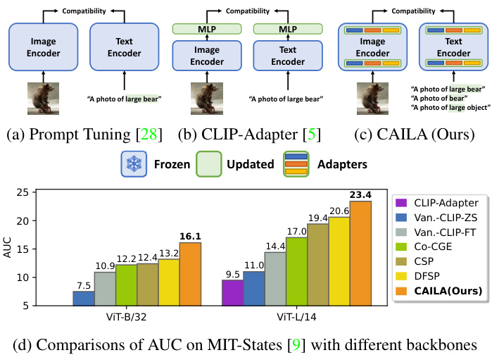
Figure 1. Illustrations of CAILA and previous CLIP-based baselines. CAILA has adapters integrated into both CLIP encoders and thus better transfers the knowledge from CLIP to CZSL, resulting in significant performance boosts compared with other CLIP-based baseline methods. “Van.-CLIP” refers to models with vanilla CLIP architecture. Prompts highlighted in green are set to be learnable parameters.
图 1: CAILA与现有基于CLIP的基线方法对比示意图。CAILA在CLIP双编码器中集成了适配器模块,能更高效地将CLIP知识迁移至CZSL任务,相比其他基于CLIP的基线方法实现了显著性能提升。"Van.-CLIP"指采用原始CLIP架构的模型。绿色高亮的提示词设为可学习参数。
1. Introduction
1. 引言
When facing a novel concept such as a large castle, humans can deconstruct individual components (large and castle) from familiar concepts (large bear, old castle) to comprehend the new composition. Such task of recognizing new attribute-object compositions based on a set of observed pairs is Compositional Zero-Shot Learning (CZSL) [24], a sine qua non for an intelligent entity. However, the inherent challenge in CZSL lies in the capacity to identify unobserved novel compositions without compromising the recognition of previously observed combinations. Conventional approaches [1, 19, 20, 23–27, 31, 35, 39, 40, 43] often suffer from training biases. Even though recent methods employ large-scale Vision-Language Pre-training (VLP)
面对诸如"大型城堡"这样的新概念时,人类能够从熟悉的概念(大型熊、古老城堡)中解构出单个要素(大型、城堡)来理解新的组合。这种基于一组已观察到的属性-对象对来识别新组合的任务被称为组合零样本学习 (CZSL) [24],是智能实体的必备能力。然而,CZSL的内在挑战在于识别未观测到的新组合时,不能损害对已观测组合的识别能力。传统方法 [1, 19, 20, 23–27, 31, 35, 39, 40, 43] 往往受困于训练偏差。尽管近期方法采用了大规规模视觉语言预训练 (VLP)
models with strong generalization ability, e.g., CLIP [32], to accommodate this issue, they simply treat VLP models as frozen black box encoders and fail to exploit the potential of VLP models. Thus, here, we explore how to more effectively extract and utilize the knowledge embedded in pre-trained vision-language models for the recognition of novel attribute-object compositions.
具有强大泛化能力的模型(如CLIP [32])来解决这一问题,他们仅将视觉语言预训练(VLP)模型视为冻结的黑盒编码器,未能充分挖掘其潜力。因此,我们在此探索如何更有效地提取和利用预训练视觉语言模型中嵌入的知识,以识别新颖的属性-对象组合。
More specifically, to adapt VLP models for CZSL, some researchers apply prompt-tuning [28,47,48] or fine-tune the model with extra adaptation layers [5] on the top of CLIP. However, prompt-tuning methods, depicted in Figure 1(a), only learn trainable prompts, while CLIP-Adapter, shown in Figure 1(b), only adds external modules outside CLIP. Both strategies abstain from altering the fundamental CLIP encoder, consequently retaining CLIP as a static black box. Nayak et al. [28] have shown that exhaustively fine-tuning CLIP falls short of attaining practicable performance. Thus, we argue that properly optimizing features across layers through a task-specific design is critical to effectively harnessing the knowledge embedded in CLIP. A feasible CLIPbased CZSL should: i) have task-specific designs for CZSL; ii) be capable of extracting concept-specific features related to compositions and individual primitives.
具体来说,为了让视觉语言预训练 (VLP) 模型适应组合零样本学习 (CZSL),一些研究者在 CLIP 基础上采用提示调优 [28,47,48] 或通过额外适配层微调模型 [5]。然而,如图 1(a) 所示的提示调优方法仅学习可训练提示词,而图 1(b) 所示的 CLIP-Adapter 仅在 CLIP 外部添加模块。这两种策略都避免改动 CLIP 编码器核心结构,导致 CLIP 始终作为静态黑箱运行。Nayak 等人 [28] 已证明,对 CLIP 进行全参数微调难以达到实用性能。因此我们认为,通过任务定制化设计对各层特征进行合理优化,对有效利用 CLIP 内嵌知识至关重要。一个可行的基于 CLIP 的 CZSL 方案应满足:i) 具有针对 CZSL 的任务定制设计;ii) 能提取与组合体及其组成元素相关的概念特异性特征。
Hence, we propose CAILA , Concept-Aware IntraLayer Adapters, that satisfy the given prerequisites and substantiate its superiority, as shown in Fig. 1(d), compared with other CLIP-based methods. Fig. 1(c) highlights the difference between CAILA and other VLP-based methods. Instead of prompt tuning or fully fine-tuning, we adopt adapters [7] to transfer knowledge from VLP models while avoiding strong training biases.
因此,我们提出CAILA(概念感知层内适配器),它满足给定的前提条件,并证实了其优越性,如图1(d)所示,与其他基于CLIP的方法相比。图1(c)突出了CAILA与其他基于视觉语言预训练(VLP)方法的区别。我们采用适配器[7]来迁移VLP模型的知识,而非提示调优或完全微调,从而避免强烈的训练偏差。
Moreover, given that adapters are low-overhead components, it is feasible to employ a variety of adapters to extract concept-wise representations. More specifically, CAILA integrates a group of adapters into each layer of both encoders; each group possesses concept-specific components to extract knowledge corresponding to particular concepts, including attributes, objects, and compositions. To merge features extracted by various concept-aware adapters, we propose the Mixture-of-Adapters (MoA) mechanism for both vision and yrcy encoder. In addition, the property that CAILA can extract concept-specific features allows us to further propose Primitive Concept Shift, which generates additional vision embeddings by combining the attribute feature from one image and the object feature from another for a more comprehensive understanding.
此外,考虑到适配器是低开销组件,采用多种适配器提取概念级表征是可行的。具体而言,CAILA在双编码器的每一层都集成了一组适配器,每组包含针对特定概念(如属性、对象及组合)的专用组件以提取相应知识。为融合不同概念感知适配器提取的特征,我们为视觉和yrcy编码器提出了混合适配器(Mixture-of-Adapters,MoA)机制。此外,CAILA能提取概念特异性特征的性质,使我们进一步提出原始概念迁移(Primitive Concept Shift),该方法通过组合一张图像的属性特征与另一张图像的对象特征来生成额外的视觉嵌入,以实现更全面的理解。
We evaluate our approach on three popular CZSL datasets: MIT-States [9], C-GQA [25] and UT-Zappos [44, 45], under both closed world and open world settings. We also report the performance of CAILA in closed world on VAW-CZSL [35], a newly released benchmark. Our experiments show that, in both scenarios, our model beats the state-of-the-arts over all benchmarks following the generalized evaluation protocol [31], by significant margins.
我们在三个流行的组合零样本学习(CZSL)数据集上评估了我们的方法:MIT-States [9]、C-GQA [25] 和 UT-Zappos [44,45],涵盖封闭世界和开放世界两种设定。同时,我们在新发布的VAW-CZSL [35]基准测试中报告了CAILA在封闭世界下的性能。实验表明,在广义评估协议[31]框架下,我们的模型在所有基准测试中都显著超越了当前最优方法。
To summarize, our contributions are as follows: (i) We propose CAILA, which is the first model exploring CZSLoriented designs with CLIP models to balance model capacity and training bias robustness; (ii) we design the Mixtureof-Adapter (MoA) mechanism to fuse the knowledge from concept-aware adapters and improve the general iz ability; (iii) we further enrich the training data and exploit the power of CAILA through Primitive Concept Shifts; (iv) we conduct extensive experiments in exploring the optimal setup for CAILA on CZSL. Quantitative experiments show that our model outperforms the SOTA by significant margins in both closed world and open world, on all benchmarks.
总结来说,我们的贡献如下:(i) 我们提出了CAILA,这是首个探索面向CZSL(组合零样本学习)设计并与CLIP模型结合以平衡模型容量和训练偏差鲁棒性的模型;(ii) 我们设计了混合适配器(Mixture-of-Adapter,MoA)机制,用于融合概念感知适配器的知识并提升泛化能力;(iii) 我们通过原始概念迁移(Primitive Concept Shifts)进一步丰富了训练数据并充分发挥了CAILA的潜力;(iv) 我们在CZSL上进行了大量实验以探索CAILA的最佳配置。定量实验表明,我们的模型在闭集和开集场景下的所有基准测试中均显著优于当前最优方法(SOTA)。
2. Related Works
2. 相关工作
Zero-Shot Learning (ZSL). Unlike conventional fullysupervised learning, ZSL requires models to learn from side information without observing any visual training samples [16]. The side information comes from multiple non-visual resources such as attributes [16], word embeddings [36, 38] , and text descriptions [33]. Notably, Zhang et al. [46] propose to learn a deep embedding model bridging the seen and the unseen, while [2,42,49] investigate generative models that produce features for novel categories. Moreover, [11, 38] integrate Graph Convolution Networks (GCN) [15] to better generalize over unseen categories.
零样本学习 (ZSL) 。与传统全监督学习不同,零样本学习要求模型在不观察任何视觉训练样本的情况下从辅助信息中学习 [16] 。这些辅助信息来自多种非视觉资源,例如属性 [16] 、词嵌入 [36, 38] 和文本描述 [33] 。值得注意的是,Zhang 等人 [46] 提出学习一个深度嵌入模型来连接已知和未知类别,而 [2,42,49] 则研究了为新颖类别生成特征的生成式模型。此外,[11, 38] 整合了图卷积网络 (GCN) [15] 以更好地泛化到未见类别。
Compost ional Zero-Shot Learning (CZSL). Previous CZSL approaches are built with pre-trained image encoders, e.g. ResNet and separate word embeddings, e.g. GloVe [30]. More specifically, Li et al. [20] investigate the symmetrical property between objects and attributes, while Atzmon et al. [1] study the casual influence between the two. Moreover, Li et al. [19] construct a Siamese network with contrastive learning to learn better object/attribute prototypes. On the other hand, joint representations of compositions can be leveraged in multiple ways. [31] utilizes joint embeddings to control gating functions for the modular network, while [26, 27, 40, 43] treat them as categorical centers in the joint latent space. Furthermore, some approaches [23–25,34,39] directly take compositional embeddings as classifier weights, while OADis [35] disentangles attributes and objects in the visual space.
组合式零样本学习 (CZSL)。现有的CZSL方法通常采用预训练图像编码器(如ResNet)和独立词嵌入(如GloVe [30])构建。具体而言,Li等人[20]研究了物体与属性间的对称性关系,Atzmon等人[1]则探讨了两者间的因果影响。此外,Li等人[19]通过构建对比学习的连体网络来优化物体/属性原型学习。另一方面,组合表征可通过多种方式加以利用:[31]采用联合嵌入控制模块化网络的门控函数,而[26,27,40,43]将其视为联合潜在空间中的分类中心。另有方法[23-25,34,39]直接将组合嵌入作为分类器权重,OADis[35]则实现了视觉空间中属性与物体的解耦。
Parameter-Efficient Tuning. Recent research on large scale pre-training models [6, 8, 10, 18, 32] has achieved superior performance on various downstream tasks, compared with regular approaches. Various works [7,12,37] show that tuning adapters [7] on the language side yields comparable results with fully fine-tuned variants, while Chen et al. [3] investigate the adaptation of image encoders on dense prediction tasks. For CZSL, a few models [28, 48] leverage the knowledge of CLIP through prompt tuning [17] , while Gao et al. [5] attach a post-processor to CLIP for knowledge transfer. Though these methods show strong performance on CZSL against regular models, they treat the CLIP model as a black box and keep it completely frozen. In CAILA , we open up the CLIP black box by integrating intra-layer adapters to both image and text encoders.
参数高效调优。近期关于大规模预训练模型[6,8,10,18,32]的研究表明,相比常规方法,这些模型在各种下游任务中表现更优。多项工作[7,12,37]指出,仅对语言侧适配器(adapter)[7]进行调优即可获得与全参数微调相当的效果,而Chen等人[3]则研究了图像编码器在密集预测任务中的适配方法。在CZSL领域,部分模型[28,48]通过提示调优(prompt tuning)[17]利用CLIP的知识,Gao等人[5]则为CLIP添加后处理器实现知识迁移。尽管这些方法在CZSL任务中展现出优于常规模型的性能,但它们都将CLIP视为黑箱并保持完全冻结状态。在CAILA中,我们通过向图像和文本编码器集成层内适配器,打开了CLIP的黑箱结构。
3. Approach
3. 方法
The problem of CZSL can be formulated as follows. We denote the training set by $\mathcal T={(x,y)|x\in\mathcal X,y\in\mathcal V_{s}}$ , where $\mathcal{X}$ contains images represented in the RGB color space and $\mathcal{D}{s}$ is a set of seen composition labels which are available during the training phase. Each label $y=(a,o)$ is a pair of attribute $a\in A$ and object category $o\in\mathcal{O}$ . When testing, CZSL expects models to predict a set of unseen compositions ${\mathcal{V}}{u}$ that is mutually exclusive with training labels $\mathcal{D}{s}$ : $\mathcal{V}{s}\cup\mathcal{V}{u}=\emptyset$ . Note that $\mathcal{D}{s}$ and ${\mathcal{V}}{u}$ share the same set of $A,{\mathcal{O}}$ , while CZSL assumes that each $a\in{\mathcal{A}}$ or $o\in\mathcal{O}$ exists in the training set and only the composition $(a,o)\in\mathcal{Y}{u}$ is novel. Following [25, 31, 41], we focus on generalized CZSL, where the test set contains both seen and unseen labels, formally denoted by $\mathcal{V}{t e s t}=\mathcal{V}{s}\cup\mathcal{V}_{u}$ .
CZSL问题可以表述如下。我们将训练集表示为$\mathcal T={(x,y)|x\in\mathcal X,y\in\mathcal V_{s}}$,其中$\mathcal{X}$包含RGB色彩空间表示的图像,$\mathcal{D}{s}$是训练阶段可见的组合标签集合。每个标签$y=(a,o)$由属性$a\in A$和物体类别$o\in\mathcal{O}$组成。测试时,CZSL要求模型预测与训练标签$\mathcal{D}{s}$互斥的未见组合集合${\mathcal{V}}{u}$:$\mathcal{V}{s}\cup\mathcal{V}{u}=\emptyset$。需注意$\mathcal{D}{s}$和${\mathcal{V}}{u}$共享相同的$A,{\mathcal{O}}$集合,且CZSL假设每个$a\in{\mathcal{A}}$或$o\in\mathcal{O}$在训练集中存在,仅组合$(a,o)\in\mathcal{Y}{u}$是新颖的。根据[25,31,41],我们关注广义CZSL场景,其测试集同时包含可见与未见标签,形式化表示为$\mathcal{V}{t e s t}=\mathcal{V}{s}\cup\mathcal{V}_{u}$。
Most recent works [1,25,31] study the generalized CZSL problem under the closed world setting, where $\mathcal{D}{t e s t}$ is a subset of the complete composition set $y:{\mathcal{A}}\times{\mathcal{O}}$ . The closed world setting assumes that ${\mathcal{V}}{u}$ are known during testing and thus greatly reduce the size of the search space. On the contrary, Mancini et al. [22] argue that such constraint should not be applied to the search space and introduce the open world setting, where models are required to search over the complete set of compositions, formally $\mathcal{Y}{s}\cup\mathcal{Y}_{u}=\mathcal{Y}$ . In this paper, we investigate the problem in both closed world and open world.
大多数最新研究[1,25,31]都在封闭世界设定下研究广义CZSL问题,其中$\mathcal{D}{t e s t}$是完整组合集$y:{\mathcal{A}}\times{\mathcal{O}}$的子集。封闭世界设定假设测试期间已知${\mathcal{V}}{u}$,从而大幅缩小了搜索空间。相反,Mancini等人[22]认为这种限制不应施加于搜索空间,并提出了开放世界设定,要求模型在整个组合集上进行搜索,即$\mathcal{Y}{s}\cup\mathcal{Y}_{u}=\mathcal{Y}$。本文将在封闭世界和开放世界两种设定下研究该问题。
3.1. Compatibility Estimation Pipeline
3.1. 兼容性评估流程
As different attributes can lead to significant appearance shifts even inside the same object category, performing attribute and object predictions separately may be ineffective. Hence, we model attribute-object compositions jointly and learn a combined estimation function to measure the compatibility of input image $x$ and query composition $(a,o)$ . In addition, we let the model estimate attribute and object comp a tibi li ties as auxiliary sub-tasks during training.
由于同一物体类别内不同属性可能导致显著的外观变化,单独预测属性和物体可能效果不佳。因此,我们联合建模属性-物体组合,并学习一个联合估计函数来衡量输入图像$x$与查询组合$(a,o)$的兼容性。此外,我们让模型在训练过程中将属性和物体兼容性估计作为辅助子任务。
The estimation of composition compatibility is represented as $\mathcal{C}(\boldsymbol{x},\boldsymbol{a},\boldsymbol{o}):\boldsymbol{\mathcal{X}}\times\boldsymbol{\mathcal{A}}\times\boldsymbol{\mathcal{O}}\rightarrow\mathbb{R}$ . It contains two components: The image feature extractor $\mathcal{F}{C}:\mathbb{R}^{H\times W\times3}\rightarrow\mathbb{R}^{d}$ and the text embedding generator $\mathcal{G}:\mathcal{A}\times\mathcal{O}\rightarrow\mathbb{R}^{d}$ . Note that $d$ denotes the number of channels that each representation has. Given an image $x$ and a composition $(a,o)$ , the compatibility score is defined as the dot product of $\mathcal{F}_{C}(\boldsymbol{x})$ and $\mathcal{G}(a,o)$ , formally
组合兼容性估计表示为 $\mathcal{C}(\boldsymbol{x},\boldsymbol{a},\boldsymbol{o}):\boldsymbol{\mathcal{X}}\times\boldsymbol{\mathcal{A}}\times\boldsymbol{\mathcal{O}}\rightarrow\mathbb{R}$。它包含两个组件:图像特征提取器 $\mathcal{F}{C}:\mathbb{R}^{H\times W\times3}\rightarrow\mathbb{R}^{d}$ 和文本嵌入生成器 $\mathcal{G}:\mathcal{A}\times\mathcal{O}\rightarrow\mathbb{R}^{d}$。注意 $d$ 表示每个表征的通道数。给定图像 $x$ 和组合 $(a,o)$,兼容性得分定义为 $\mathcal{F}_{C}(\boldsymbol{x})$ 与 $\mathcal{G}(a,o)$ 的点积,形式化表示为
$$
\begin{array}{r}{\mathcal{C}(\boldsymbol{x},\boldsymbol{a},\boldsymbol{o})=\mathcal{F}_{C}(\boldsymbol{x})\cdot\mathcal{G}(\boldsymbol{a},\boldsymbol{o}).}\end{array}
$$
$$
\begin{array}{r}{\mathcal{C}(\boldsymbol{x},\boldsymbol{a},\boldsymbol{o})=\mathcal{F}_{C}(\boldsymbol{x})\cdot\mathcal{G}(\boldsymbol{a},\boldsymbol{o}).}\end{array}
$$
Furthermore, as CZSL requires models to recognize novel pairs composed of known attributes and objects, it is important for a model to possess the capability of primitive feature extraction that is disentangled with training compositions. Thus, we make our model extract features corresponding to primitives and estimate the compatibility between vision features and text representations during training. Similar to Eqn. 1, we have
此外,由于CZSL要求模型识别由已知属性和对象组成的新颖组合,模型必须具备与训练组合解耦的基元特征提取能力。因此,我们让模型在训练过程中提取与基元对应的特征,并评估视觉特征与文本表征之间的兼容性。类似于公式1,我们有
$$
{\mathcal{C}}(x,a)={\mathcal{F}}{A}(x)\cdot{\mathcal{G}}{A}(a),{\mathcal{C}}(x,o)={\mathcal{F}}{O}(x)\cdot{\mathcal{G}}_{O}(o).
$$
$$
{\mathcal{C}}(x,a)={\mathcal{F}}{A}(x)\cdot{\mathcal{G}}{A}(a),{\mathcal{C}}(x,o)={\mathcal{F}}{O}(x)\cdot{\mathcal{G}}_{O}(o).
$$
All three compatibility scores contribute independently to the loss function, while $\mathcal{C}(\boldsymbol{x},\boldsymbol{a},o)$ is leveraged during inference. More specifically, our framework learns separate representations through CAILA discussed in Sec. 3.2 and conducts knowledge fusion through Mixture-of-Adapters (MoA), which will be covered in Sec. 3.3.
三个兼容性分数独立贡献于损失函数,而推理过程中会利用 $\mathcal{C}(\boldsymbol{x},\boldsymbol{a},o)$。具体而言,我们的框架通过第3.2节讨论的CAILA学习独立表征,并通过第3.3节将介绍的混合适配器 (Mixture-of-Adapters, MoA) 进行知识融合。
Following [32], we create a prompt template similar to $"a$ photo of [CLASS]" for each compatibility estimation sub-task. For composition compatibility, we feed the text encoder with "a photo of [ATTRIBUTE] [OBJECT]"; We use "a photo of [ATTRIBUTE] object" and $"a$ photo of [OBJECT]" for attribute and object comp a tibi li ties, respectively. Similar to [28], we only make [CLASS] prompts trainable. For both encoders $\mathcal{F}$ and $\mathcal{G}$ , we take the output hidden state of the [CLS] token as the representation.
遵循[32]的方法,我们为每个兼容性评估子任务创建了类似 $"a$ photo of [CLASS]" 的提示模板。对于组合兼容性,我们将"a photo of [ATTRIBUTE] [OBJECT]"输入文本编码器;分别使用"a photo of [ATTRIBUTE] object"和 $"a$ photo of [OBJECT]"来评估属性和对象兼容性。与[28]类似,我们仅使[CLASS]提示可训练。对于编码器 $\mathcal{F}$ 和 $\mathcal{G}$,我们取[CLS] token的输出隐藏状态作为表征。
3.2. Concept-Aware Intra-Layer Adapters
3.2. 概念感知层内适配器
Though CLIP-based CZSL approaches [5, 28, 48] have achieved significant improvements compared with earlier methods [22, 24, 25, 28, 31], the CLIP encoder is considered as a black box and no modifications are made to improve its general iz ability. Thus, we propose to improve CLIP-based CZSL models in both modalities with CAILA , ConceptAware Intra-Layer Adapters.
尽管基于CLIP的CZSL方法[5, 28, 48]相比早期方法[22, 24, 25, 28, 31]取得了显著改进,但CLIP编码器被视为黑箱且未进行改进以提升其泛化能力。为此,我们提出通过CAILA (ConceptAware Intra-Layer Adapters) 在双模态中改进基于CLIP的CZSL模型。
As shown in Fig. 2 (a)(b), we take the CLIP image encoder as $\mathcal{F}$ and the text encoder as $\mathcal{G}$ , while adding concept awareness to both encoders when estimating comp a tibi li ties of different concepts. Fig. 2 (c) demonstrates how adapters are integrated into a regular transformer encoding block. For each encoding block, we add adapters behind the frozen self-attention layer and the feed-forward network. More specifically, given the input hidden state h of an adapter, we compute the latent feature $\mathbf{z}$ by the down sampling operator $f_{D o w n}$ , followed by the activation function $\sigma$ . The output $\mathbf{h}^{\prime}$ of an adapter is obtained by upscaling $\mathbf{z}$ and summing it with $\mathbf{h}$ through the skip connection. Formally, we have
如图 2(a)(b)所示, 我们将 CLIP 图像编码器作为 $\mathcal{F}$, 文本编码器作为 $\mathcal{G}$, 同时在估计不同概念的兼容性时为两个编码器添加概念感知能力。图 2(c)展示了适配器如何集成到常规的 Transformer 编码块中。对于每个编码块, 我们在冻结的自注意力层和前馈网络之后添加适配器。具体来说, 给定适配器的输入隐藏状态 h, 我们通过下采样算子 $f_{Down}$ 计算潜在特征 $\mathbf{z}$, 然后经过激活函数 $\sigma$。适配器的输出 $\mathbf{h}^{\prime}$ 是通过对 $\mathbf{z}$ 进行上采样并通过跳跃连接与 $\mathbf{h}$ 相加得到的。形式上, 我们有
$$
\mathbf{z}=\sigma(f_{D o w n}(\mathbf{h})),\quad\mathbf{h}^{\prime}=f_{U p}(\mathbf{z})+\mathbf{h},
$$
$$
\mathbf{z}=\sigma(f_{D o w n}(\mathbf{h})),\quad\mathbf{h}^{\prime}=f_{U p}(\mathbf{z})+\mathbf{h},
$$
where both $f_{D o w n}$ and $f_{U p}$ are fully-connected layers.
其中 $f_{D o w n}$ 和 $f_{U p}$ 均为全连接层。
To extract concept-specific features, at each depth level, we create three encoding blocks corresponding to attribute, object, and composition, respectively. As in Fig. 2(c), encoding blocks of at the same level share the same weights except for the adapter layers. Inputs from both modalities are processed by encoders equipped with different types of encoding blocks and features related to each of the three concepts are produced. During training, vision-language compatibility scores for “attribute”, “object” and “compositions” are estimated. More specifically, encoders referred in Fig. 2(a) and (b) are the same ones; There are not extra side encoders for auxiliary sub-tasks.
为了提取特定概念的特征,我们在每个深度级别分别创建了对应于属性(attribute)、对象(object)和组合(composition)的三个编码块。如图 2(c)所示,同一层级的编码块除了适配器层外共享相同权重。来自两种模态的输入会经过配备不同类型编码块的编码器处理,生成与三个概念各自相关的特征。在训练过程中,我们会估算"属性"、"对象"和"组合"的视觉-语言兼容性分数。更具体地说,图 2(a)和(b)中提到的编码器是相同的;没有为辅助子任务设置额外的旁路编码器。
3.3. MoA: Mixture of Adapters
3.3. MoA: 混合适配器 (Mixture of Adapters)
To aggregate the knowledge extracted by adapters corresponding to attributes, objects, and compositions, we propose Mixture-of-Adapters mechanisms for both the vision side and language side of the encoder.
为了整合由适配器提取的与属性、物体和组合相对应的知识,我们在编码器的视觉端和语言端均提出了混合适配器(Mixture-of-Adapters)机制。
On the vision side, we perform a two-stage feature extraction. As shown in Fig. 2 (a), for the first $N_{V}-M$ layers, we extract features related to the attribute $(\mathbf{h}{A})$ and the object $(\mathbf{h}{O})$ through corresponding encoding blocks, which are further concatenated and processed by the trailing $M$ ternary MoA layers. An example of the vision MoA layer is shown in Fig. 3. Given the hidden state $h$ , we extract latent features $\mathbf{z}{\mathbf{A}},\mathbf{z}{\mathbf{O}}$ and $\mathbf{z}{\mathbf{C}}$ from the adapters. We then combine all three features and create $\mathbf{z_{C}^{\prime}}$ , followed by $f_{U p}$ :
在视觉方面,我们采用两阶段特征提取方法。如图2(a)所示,前$N_{V}-M$层通过对应的编码块提取与属性$(\mathbf{h}{A})$和对象$(\mathbf{h}{O})$相关的特征,这些特征经过拼接后由后续$M$个三元MoA层处理。图3展示了视觉MoA层的示例。给定隐藏状态$h$,我们从适配器中提取潜在特征$\mathbf{z}{\mathbf{A}}$、$\mathbf{z}{\mathbf{O}}$和$\mathbf{z}{\mathbf{C}}$。随后将三个特征组合生成$\mathbf{z_{C}^{\prime}}$,再经过$f_{U p}$处理:
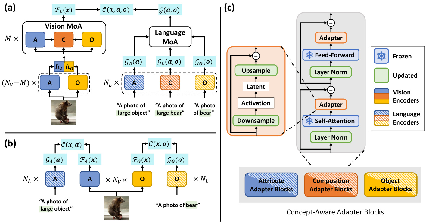
Figure 2. An overview of CAILA $:$ (a) The main composition compatibility estimation pipeline; (b) Auxiliary sub-tasks on primitive compatibility during training; (c) The structure of CAILA layers. Our model extracts concept-specific features by learning different adapters and fuses them through the Mixture-of-Adapters (MoA) mechanism. Note that for each layer of encoders in (a) and (b), the weights of encoding blocks of the same concept are shared. $N_{V},N_{L}$ and $M$ indicate numbers of layers.
图 2: CAILA 概述:(a) 主要成分兼容性评估流程;(b) 训练期间关于原始兼容性的辅助子任务;(c) CAILA 层的结构。我们的模型通过学习不同的适配器提取特定概念的特征,并通过混合适配器 (Mixture-of-Adapters, MoA) 机制进行融合。注意在 (a) 和 (b) 中,同一概念的编码块权重在各编码器层间共享。$N_{V}$、$N_{L}$ 和 $M$ 表示层数。
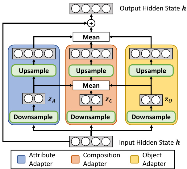
Figure 3. Details of our vision Mixture-of-Adapter. Latent features of each adapter, $\mathbf{z}{\mathbf{A}},\mathbf{z}{\mathbf{O}},\mathbf{z}{\mathbf{C}}$ , are mixed, and further processed by the upsampling function to generate $\mathbf{h_{C}^{\prime}}$ . $\mathbf{h_{C}^{\prime}}$ is joined with $\mathbf{h}{\mathbf{A}}^{\prime},\mathbf{h}{\mathbf{O}}^{\prime}$ and input feature $\mathbf{h}$ for output.
图 3: 视觉混合适配器 (Mixture-of-Adapter) 的详细结构。每个适配器的潜在特征 $\mathbf{z}{\mathbf{A}},\mathbf{z}{\mathbf{O}},\mathbf{z}{\mathbf{C}}$ 经过混合后,通过上采样函数进一步处理生成 $\mathbf{h_{C}^{\prime}}$ 。 $\mathbf{h_{C}^{\prime}}$ 与 $\mathbf{h}{\mathbf{A}}^{\prime},\mathbf{h}_{\mathbf{O}}^{\prime}$ 及输入特征 $\mathbf{h}$ 拼接后输出。
$$
\begin{array}{r}{\mathbf{z}{\mathbf{C}}^{\prime}=\mathrm{Avg}\left[\mathbf{z}{\mathbf{A}},\mathbf{z}{\mathbf{O}},\mathbf{z}{\mathbf{C}}\right],\quad\mathbf{h}{\mathbf{C}}^{\prime}=f_{U p}(\mathbf{z}_{\mathbf{C}}^{\prime}).}\end{array}
$$
$$
\begin{array}{r}{\mathbf{z}{\mathbf{C}}^{\prime}=\mathrm{Avg}\left[\mathbf{z}{\mathbf{A}},\mathbf{z}{\mathbf{O}},\mathbf{z}{\mathbf{C}}\right],\quad\mathbf{h}{\mathbf{C}}^{\prime}=f_{U p}(\mathbf{z}_{\mathbf{C}}^{\prime}).}\end{array}
$$
We further combine $\mathbf{h_{C}^{\prime}}$ with outputs of attribute and object adapters, $\mathbf{h_{A}^{\prime}}$ and $\mathbf{h}_{\mathbf{O}}^{\prime}$ , to create the output:
我们进一步将 $\mathbf{h_{C}^{\prime}}$ 与属性和对象适配器的输出 $\mathbf{h_{A}^{\prime}}$ 和 $\mathbf{h}_{\mathbf{O}}^{\prime}$ 结合,生成最终输出:
$$
\mathbf{h}^{\prime}=\operatorname{Avg}\left[\mathbf{h}{\mathbf{A}}^{\prime},\mathbf{h}{\mathbf{O}}^{\prime},\mathbf{h}_{\mathbf{C}}^{\prime}\right]+\mathbf{h}.
$$
$$
\mathbf{h}^{\prime}=\operatorname{Avg}\left[\mathbf{h}{\mathbf{A}}^{\prime},\mathbf{h}{\mathbf{O}}^{\prime},\mathbf{h}_{\mathbf{C}}^{\prime}\right]+\mathbf{h}.
$$
The output of the last mixture layer is L2-normalized and adopted as $\mathcal{F}_{C}(\boldsymbol{x})$ for compatibility estimation. Ablation study on this module is discussed in Sec. 4.3.
最后一层混合层的输出经过L2归一化后作为$\mathcal{F}_{C}(\boldsymbol{x})$用于兼容性估计。该模块的消融研究将在第4.3节讨论。
Unlike the vision side, where attributes and objects are deeply entangled within the same input image. On the language side, we can create disentangled language inputs through different prompt templates for attributes and objects separately. Thus, we adopt a simple mixture strategy for language adapters. We compute the compositional embedding through $N_{L}$ encoding blocks for the composition and combine it with primitive language embeddings:
与视觉端不同,视觉端的属性和对象在同一输入图像中深度纠缠。而在语言端,我们可以通过不同的提示模板分别为属性和对象创建解耦的语言输入。因此,我们对语言适配器采用简单的混合策略。通过 $N_{L}$ 个编码块计算组合嵌入,并将其与原始语言嵌入相结合:
$$
\mathcal{G}(a,o)=\mathrm{Avg}\big[\mathcal{G}{A}(a),\mathcal{G}{O}(o),\mathcal{G}_{C}(a,o)\big].
$$
$$
\mathcal{G}(a,o)=\mathrm{Avg}\big[\mathcal{G}{A}(a),\mathcal{G}{O}(o),\mathcal{G}_{C}(a,o)\big].
$$
3.4. Primitive Concept Shift on Image Embeddings
3.4. 图像嵌入的原始概念偏移
Due to the limited diversity of training data, current CZSL models often suffer from training biases. As discussed in Sec. 3.3, in addition to the composition-related feature, CAILA extracts attribute- and object-oriented features during the first stage of $\mathcal{F}_{C}$ . That motivates us to leverage these primitive-specific features to create additional embeddings for certain compositions. As it leads to changes in labels of original images, e.g. from melted butter to melted candy, we call it primitive concept shift.
由于训练数据多样性有限,当前的CZSL模型常受训练偏差影响。如第3.3节所述,CAILA在$\mathcal{F}_{C}$第一阶段除了提取组合相关特征外,还会提取面向属性和对象的特征。这促使我们利用这些原始特征为特定组合创建额外嵌入。由于该操作会导致原始图像标签变化(例如从"融化的黄油"变为"融化的糖果"),我们将其称为原始概念迁移。
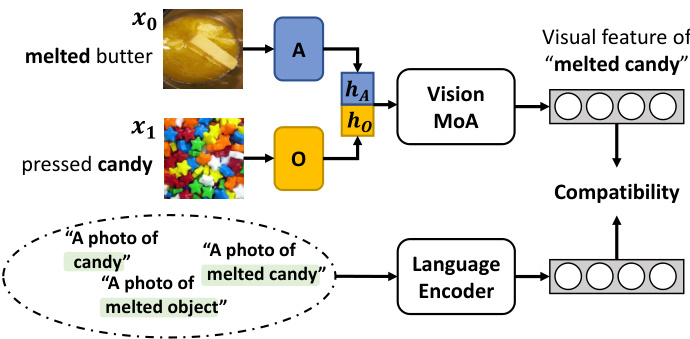
Figure 4. Illustrations of concept shift. We perform concept shift by combining the attribute (melted) feature from one image with the object (candy) feature to create an additional composition (melted candy) feature. Newly generated features are shuffled with regular samples during training.
图 4: 概念漂移示意图。我们通过将一幅图像的属性特征(融化态)与另一幅图像的对象特征(糖果)结合,创建出新的组合特征(融化糖果)。训练过程中,这些新生成的特征会与常规样本进行随机混合。
Fig. 4 demonstrates the process of concept shift: Given one sample $x_{0}$ of melted butter and one sample $x_{1}$ of pressed candy, we create a new sample of melted candy in the feature space, by combining the attributeoriented feature $\mathbf{h}{A}$ of $x_{0}$ and the object-oriented feature $\mathbf{h}{O}$ of $x_{1}$ . The newly combined feature is further processed by vision MoA layers described in Sec. 3.3, leading to an embedding representing melted candy. Such change can be viewed as an “object shift” from melted butter or an “attribute shift” from pressed candy. Thus, we name this process “primitive concept shift”. In practice, we randomly pick a proportion of samples for shifting and ensure that the new label after shifting still lies in the training set. We discuss the effectiveness of the shifting in Sec .4.3.
图 4 展示了概念迁移的过程:给定一个融化黄油样本 $x_{0}$ 和一个压榨糖果样本 $x_{1}$ ,我们通过在特征空间中结合 $x_{0}$ 的属性导向特征 $\mathbf{h}{A}$ 和 $x_{1}$ 的对象导向特征 $\mathbf{h}_{O}$ ,创建出一个融化糖果的新样本。新组合的特征会经过第3.3节描述的视觉MoA层进一步处理,最终生成代表融化糖果的嵌入表示。这种变化既可以视为从融化黄油发生的"对象迁移",也可以看作从压榨糖果发生的"属性迁移"。因此,我们将此过程命名为"原始概念迁移"。实际操作中,我们会随机选取部分样本进行迁移,并确保迁移后的新标签仍属于训练集范围。迁移效果的具体分析将在第4.3节展开讨论。
Although there are previous explorations [19,40] in generating novel features in the latent space, our method is essentially novel from two aspects: i) Wei et al. [40] generate features directly from word embeddings, while our method leverages disentangled vision features that have richer and more diverse knowledge; ii) Li et al. [19] uses generated features to augment primitive vision encoders, while ours augments the entire model through CAILA for both compositions and individual primitives.
尽管先前已有研究[19,40]探索在潜在空间中生成新特征,但我们的方法在两方面具有本质创新:i) Wei等人[40]直接从词嵌入生成特征,而我们的方法利用了具有更丰富多样知识的解耦视觉特征;ii) Li等人[19]使用生成特征增强原始视觉编码器,而我们的方法通过CAILA同时增强组合结构和独立基元的整个模型。
3.5. Training and Testing
3.5. 训练与测试
Objective. We optimize our model with a main loss on attribute-object compositions and auxiliary losses on attributes and objects. As our model only has access to seen compositions $Y_{s}$ , we create our training objective upon $Y_{s}$ and ignore other compositions during training. More specifically, given an image $x$ , we compute the compatibility score $\mathcal{C}(\boldsymbol{x},\boldsymbol{a},\boldsymbol{o}),\mathcal{C}(\boldsymbol{x},\boldsymbol{a})$ and $\ensuremath{\mathcal{C}}(x,o)$ for all $(a,o)\in Y_{s}$ . We then jointly optimize $\mathcal{F}$ and $\mathcal{G}$ by the cross-entropy loss with
目标。我们通过主损失函数优化属性-对象组合,并通过辅助损失函数优化属性和对象。由于模型仅能接触已见组合 $Y_{s}$,因此训练目标基于 $Y_{s}$ 构建,训练期间忽略其他组合。具体而言,给定图像 $x$,我们为所有 $(a,o)\in Y_{s}$ 计算兼容性得分 $\mathcal{C}(\boldsymbol{x},\boldsymbol{a},\boldsymbol{o})$、$\mathcal{C}(\boldsymbol{x},\boldsymbol{a})$ 和 $\ensuremath{\mathcal{C}}(x,o)$。随后通过交叉熵损失联合优化 $\mathcal{F}$ 和 $\mathcal{G}$。
temperature:
温度:
$$
\begin{array}{l}{\displaystyle\mathcal{L}=\frac{-1}{|\mathcal{T}|}\sum_{i}\bigg{\log\frac{e^{[\mathcal{C}(x_{i},a_{i},o_{i})/\tau_{C}]}}{\displaystyle\sum_{j}e^{[\mathcal{C}(x_{i},a_{j},o_{j})/\tau_{C}]}}+}\ {\log\frac{e^{[\mathcal{C}(x_{i},a_{i})/\tau_{A}]}}{\displaystyle\sum_{j}e^{[\mathcal{C}(x_{i},a_{j})/\tau_{A}]}}+\log\frac{e^{[\mathcal{C}(x_{i},o_{i})/\tau_{O}]}}{\displaystyle\sum_{j}e^{[\mathcal{C}(x_{i},o_{j})/\tau_{O}]}}\bigg}.}\end{array}
$$
$$
\begin{array}{l}{\displaystyle\mathcal{L}=\frac{-1}{|\mathcal{T}|}\sum_{i}\bigg{\log\frac{e^{[\mathcal{C}(x_{i},a_{i},o_{i})/\tau_{C}]}}{\displaystyle\sum_{j}e^{[\mathcal{C}(x_{i},a_{j},o_{j})/\tau_{C}]}}+}\ {\log\frac{e^{[\mathcal{C}(x_{i},a_{i})/\tau_{A}]}}{\displaystyle\sum_{j}e^{[\mathcal{C}(x_{i},a_{j})/\tau_{A}]}}+\log\frac{e^{[\mathcal{C}(x_{i},o_{i})/\tau_{O}]}}{\displaystyle\sum_{j}e^{[\mathcal{C}(x_{i},o_{j})/\tau_{O}]}}\bigg}.}\end{array}
$$
Intuitively, the cross-entropy loss will force the model to produce a higher compatibility score when $(x,a,o)$ matches and lower the score when a non-label composition occurs.
直观上,交叉熵损失会迫使模型在 $(x,a,o)$ 匹配时生成更高的兼容性分数,而在出现非标签组合时降低该分数。
Inference. The generalized CZSL task requires models to perform recognition over a joint set of seen and unseen compositions. Thus, for each test sample $x$ , we estimate the compatibility score between $x$ and every candidate $(a,o)$ inside the search space $\mathfrak{P}{s}\cup\mathfrak{V}_{u}$ . We predict the image $x$ as the composition that has the highest compatibility score:
推理。广义的 CZSL 任务要求模型在已见和未见组合的联合集合上进行识别。因此,对于每个测试样本 $x$,我们计算 $x$ 与搜索空间 $\mathfrak{P}{s}\cup\mathfrak{V}_{u}$ 中每个候选组合 $(a,o)$ 之间的兼容性得分。我们将图像 $x$ 预测为具有最高兼容性得分的组合:
$$
\hat{y}=\underset{(a,o)\in\mathcal{V}{s}\cup\mathcal{V}_{u}}{\arg\operatorname*{max}}~\mathcal{C}(x,a,o)
$$
$$
\hat{y}=\underset{(a,o)\in\mathcal{V}{s}\cup\mathcal{V}_{u}}{\arg\operatorname*{max}}~\mathcal{C}(x,a,o)
$$
We apply the prediction protocol to all benchmarks.
我们对所有基准测试应用了预测协议。
4. Experiments
4. 实验
4.1. Experiment Settings
4.1. 实验设置
Datasets. We evaluate CAILA on four popular datasets: MIT-States [9], C-GQA [25], UT-Zappos [44, 45] and VAW-CZSL [35]. For splits, we follow [25] for C-GQA, [35] for VAW-CZSL, and [31] for MIT-States/UT-Zappos. Statistically, the numbers of images in train/val/test are $29\mathrm{k/10k/10k}$ for MIT-States, $23\mathrm{k}/3\mathrm{k}/3\mathrm{k}$ for UT-Zappos, 26k/7k/5k for C-GQA, and $72\mathrm{k}/10\mathrm{k}/10\mathrm{k}$ for VAW-CZSL.
数据集。我们在四个常用数据集上评估CAILA:MIT-States [9]、C-GQA [25]、UT-Zappos [44, 45]和VAW-CZSL [35]。数据划分方面,C-GQA采用[25]的方案,VAW-CZSL采用[35]的方案,MIT-States/UT-Zappos采用[31]的方案。统计显示,训练集/验证集/测试集的图像数量分别为:MIT-States $29\mathrm{k/10k/10k}$,UT-Zappos $23\mathrm{k}/3\mathrm{k}/3\mathrm{k}$,C-GQA 26k/7k/5k,VAW-CZSL $72\mathrm{k}/10\mathrm{k}/10\mathrm{k}$。
Scenarios. We perform evaluation of CZSL models on both closed and open world scenarios and denote them as $\bullet$ and , respectively. Regarding the closed world setting, we follow [1, 25, 31] and conduct CZSL with a limited search space. We further run models in the open world scenario, proposed by Mancini et al. [22], to assess the s cal ability of CZSL models. It is worth noting that C-GQA becomes much more challenging under the open world setting, as the size of the search space drastically increases from 2k to nearly $400\mathrm{k\Omega}$ . We also notice similar space expansions on MIT-States, while the number of possible compositions does not increase much on UT-Zappos.
场景。我们在封闭世界和开放世界两种场景下对 CZSL 模型进行评估,分别用 $\bullet$ 和 表示。针对封闭世界设定,我们遵循 [1, 25, 31] 的方法,在有限搜索空间内进行 CZSL 实验。此外,我们采用 Mancini 等人 [22] 提出的开放世界场景来评估 CZSL 模型的扩展能力。值得注意的是,在开放世界设定下 C-GQA 的难度显著提升,其搜索空间规模从 2k 急剧扩大到近 $400\mathrm{k\Omega}$ 。我们在 MIT-States 数据集上也观察到类似的搜索空间扩张现象,而 UT-Zappos 数据集上可能的组合数量增长幅度较小。
Evaluation Metrics. Our evaluation follows the generalized CZSL protocol adopted by [1, 22, 25, 31]. [31, 41] argue that it is unreasonable to evaluate only $Y_{u}$ as significant biases enter during training and model selection. They suggest computing both seen and unseen accuracy with various bias values added to unseen categories and taking the Area Under the Curve (AUC) as the core metric. We select our models with the best AUC on val sets and report performance on test sets.
评估指标。我们的评估遵循[1, 22, 25, 31]采用的广义CZSL协议。[31, 41]指出仅评估$Y_{u}$是不合理的,因为在训练和模型选择过程中会引入显著偏差。他们建议通过向未见类别添加不同偏差值来计算已见和未见准确率,并以曲线下面积 (AUC) 作为核心指标。我们选择在验证集上具有最佳AUC的模型,并报告测试集上的性能。
Table 1. Quantitative results on generalized CZSL in closed world, all numbers are reported in percentage. S and U refer to best seen and unseen accuracy on the accuracy curve. CLIP-ZS refers to the vanilla CLIP model without fine-tuning. All CLIP-based models are run with ViT-L/14 and we conduct extensive experiments in Tab. 4. $^\dagger$ We run Co-CGE with similar CLIP features and report our best number of the model. Models published before CGE are omitted as their performances are inferior to current baselines.
表 1. 封闭世界下的广义 CZSL 定量结果,所有数值均以百分比形式呈现。S 和 U 分别表示准确率曲线上的最佳可见类和未见类准确率。CLIP-ZS 指未经微调的原始 CLIP 模型。所有基于 CLIP 的模型均采用 ViT-L/14 运行,我们在表 4 中进行了大量实验。$^\dagger$ 我们使用类似的 CLIP 特征运行 Co-CGE 并报告模型的最佳数值。CGE 之前发布的模型因性能低于当前基线而被省略。
| 封闭世界模型 | ●MIT-States | ·C-GQA | ●UT-Zappos | ||||||||||
|---|---|---|---|---|---|---|---|---|---|---|---|---|---|
| AUC (↑) | HM (↑) | S (↑) | U (↑) | AUC (↑) | HM (↑) | S (↑) | U (↑) | AUC (↑) | HM (↑) | S (↑) | U (↑) | ||
| 无 CLIP | CompCos [22] | 4.5 | 16.4 | 25.3 | 24.6 | 2.6 | 12.4 | 28.1 | 11.2 | 28.7 | 43.1 | 59.8 | 62.5 |
| ProtoProp [34] | - | - | - | - | 3.7 | 15.1 | 26.4 | 18.1 | 34.7 | 50.2 | 62.1 | 65.7 | |
| OADis [35] | 5.9 | 18.9 | 31.1 | 25.6 | - | - | - | - | 30.0 | 44.4 | 59.5 | 65.5 | |
| SCEN [19] | 5.3 | 18.4 | 29.9 | 25.2 | 2.9 | 12.4 | 28.9 | 12.1 | 32.0 | 47.8 | 63.5 | 63.1 | |
| CGE [25] | 6.5 | 21.4 | 32.8 | 28.0 | 4.2 | 15.5 | 33.5 | 16.0 | 33.5 | 60.5 | 64.5 | 71.5 | |
| Co-CGE [23] | 6.6 | 20.0 | 32.1 | 28.3 | 4.1 | 14.4 | 33.3 | 14.9 | 33.9 | 48.1 | 62.3 | 66.3 | |
| 有 CLIP | CAPE [14] | 6.7 | 20.4 | 32.1 | 28.0 | 4.6 | 16.3 | 33.0 | 16.4 | 35.2 | 49.5 | 62.3 | 68.5 |
| CLIP-ZS [32] | 11.0 | 26.1 | 30.2 | 46.0 | 1.4 | 8.6 | 7.5 | 25.0 | 5.0 | 15.6 | 15.8 | 49.1 | |
| CoOp [48] | 13.5 | 29.8 | 34.4 | 47.6 | 4.4 | 17.1 | 26.8 | 20.5 | 18.8 | 34.6 | 52.1 | 49.3 | |
| Co-CGEt [23] | 17.0 | 33.1 | 46.7 | 45.9 | 5.7 | 18.9 | 34.1 | 21.2 | 36.3 | 49.7 | 63.4 | 71.3 | |
| CSP [28] | 19.4 | 36.3 | 46.6 | 49.9 | 6.2 | 20.5 | 28.8 | 26.8 | 33.0 | 46.6 | 64.2 | 66.2 | |
| DFSP [21] | 20.6 | 37.3 | 46.9 | 52.0 | 10.5 | 27.1 | 38.2 | 32.9 | 36.0 | 47.2 | 66.7 | 71.7 | |
| CAILA (Ours) | 23.4 | 39.9 | 51.0 | 53.9 | 14.8 | 32.7 | 43.9 | 38.5 | 44.1 | 57.0 | 67.8 | 74.0 |
Table 2. Quantitative results on generalized CZSL of VAW-CZSL in closed world, all numbers are reported in percentage.
表 2. VAW-CZSL 在封闭世界下的广义 CZSL 量化结果,所有数值均以百分比形式呈现。
| 封闭世界模型 | VAW-CZSL | |
|---|---|---|
| AUC (↑) | ||
| 无 CLIP | CompCos [22] | 5.6 |
| OADis [35] CGE [25] | 6.1 5.1 | |
| 使用 CLIP | CLIP-ZS[32] | 2.6 |
| CSP [28] | 8.5 | |
| DFSP [21] | 14.1 | |
| CAILA (Ours) | 17.2 |
Furthermore, best-seen accuracy and best-unseen accuracy are calculated when other candidates are filtered out by specific bias terms. We also report best Harmonic Mean (HM), defined as $(2s e e nu n s e e n)/(s e e n+u n s e e n)$ .
此外,当其他候选对象被特定偏差项过滤掉时,会计算最佳可见准确率(best-seen accuracy)和最佳未见准确率(best-unseen accuracy)。我们还报告了最佳调和平均数(HM),其定义为 $(2s e e nu n s e e n)/(s e e n+u n s e e n)$。
Implementation Details: We build our model on the PyTorch [29] framework. As for optimization, we use Adam optimizer with a weight decay of $\mathrm{5e-5}$ . The learning rate is set to $\mathrm{2e-5}$ . The batch size is set to 32 for all three datasets. The temperature $\tau_{C},\tau_{A},\tau_{O}$ is set to 0.01, 0.0005 and 0.0005, respectively. Most of the experiments are run on two NVIDIA A100 GPUs. We the number of vision MoA layers $M$ to 6 by default. For the down sampling function $f_{D o w n}$ , we set the reduction factor to 4. Ablation stud- ies on these settings can be found in Sec 4.3.
实现细节:我们在PyTorch [29]框架上构建模型。优化方面,采用权重衰减为$\mathrm{5e-5}$的Adam优化器,学习率设为$\mathrm{2e-5}$。三个数据集的批量大小均设置为32。温度参数$\tau_{C}$、$\tau_{A}$、$\tau_{O}$分别设为0.01、0.0005和0.0005。大部分实验在两块NVIDIA A100 GPU上运行。默认设置视觉MoA层数$M$为6。降采样函数$f_{Down}$的缩减因子设为4。这些设置的消融实验详见第4.3节。
4.2. Quantitative Results
4.2. 定量结果
In this section, we present quantitative results in detail under both closed world and open world settings. Such results verify the effectiveness of our method, which surpasses the current SOTA on most metrics, in both scenarios.
在本节中,我们将详细展示封闭世界和开放世界设定下的量化结果。这些结果验证了我们的方法在两种场景下的有效性,其在多数指标上超越了当前的最先进技术 (SOTA) 。
Closed World Results. Performance of the closed world scenario are reported in Tab. 1 and 2. On MIT-States, results show that CAILA overcomes the label noise and achieves SOTA. More specifically, on AUC, we observe a $2.8%$ improvement, from $20.6%$ to $23.4%$ . Furthermore, regarding HM, CAILA achieves $39.9%$ , outperforming all baselines. When it comes to best seen and unseen accuracy, our model improves by ${\sim}4%$ and ${\sim}2%$ , respectively.
封闭世界结果。封闭世界场景的性能见表1和表2。在MIT-States数据集上,结果显示CAILA克服了标签噪声并实现了SOTA (state-of-the-art)。具体而言,在AUC指标上,我们观察到$2.8%$的提升,从$20.6%$提高到$23.4%$。此外,在HM指标上,CAILA达到$39.9%$,优于所有基线方法。在最佳可见准确率和未见准确率方面,我们的模型分别提升了${\sim}4%$和${\sim}2%$。
Our results on C-GQA further verify the advantage of CAILA, especially when the number of unseen compositions is larger. On AUC, our model achieves a $4.3%$ improvement, $40%$ of the previous SOTA, from $10.5%$ to $14.8%$ . HM is also improved by $5.6%$ . Moreover, improvements of best seen and unseen accuracy are $5.7%$ and $5.6%$ .
我们在C-GQA上的结果进一步验证了CAILA的优势,尤其是在未见组合数量较多的情况下。在AUC指标上,我们的模型实现了$4.3%$的提升(达到之前SOTA的$40%$),从$10.5%$提高到$14.8%$。HM指标也提升了$5.6%$。此外,最佳可见准确率和未见准确率分别提升了$5.7%$和$5.6%$。
UT-Zappos has much fewer attributes and object categories, compared with its counterparts, and is thus much easier, as the gap between various methods is smaller. But it is noticeable that our model, CAILA , outperforms all other baselines, with a $7.2%$ improvement on the AUC metric.
UT-Zappos 相比同类数据集具有更少的属性和对象类别,因此任务更简单,各方法间的差距也较小。但值得注意的是,我们的模型 CAILA 在所有基线方法中表现最优,在 AUC 指标上实现了 7.2% 的提升。
Moreover, on the recently released benchmark, VAWCZSL, CAILA is able to achieve noticeable improvements against baseline models, particularly the newly published method, DFSP [21]. CAILA improves the AUC by $3.1%$ while boosting the harmonic mean by $3.5%$ .
此外,在最新发布的基准测试VAWCZSL上,CAILA相较于基线模型(尤其是新发表的方法DFSP [21])取得了显著提升。CAILA将AUC提高了$3.1%$,同时将调和平均数提升了$3.5%$。
Open World Results. We further conduct experiments under the open world setting to evaluate the robustness of CAILA . Results are shown in Tab. 3. Noticeably, open world is much harder than closed world, as performance on all benchmarks drops drastically, while CAILA achieves SOTA on most metrics in this scenario without any filtering techniques adopted in the previous papers [22, 23, 28].
开放世界结果。我们进一步在开放世界设置下进行实验,以评估CAILA的鲁棒性。结果显示在表3中。值得注意的是,开放世界比封闭世界更具挑战性,因为所有基准测试的性能都大幅下降,而CAILA在未采用先前论文[22, 23, 28]中任何过滤技术的情况下,仍在该场景下的大多数指标上达到了SOTA水平。
On MIT-States, our approach greatly beats SOTA on all metrics, particularly the AUC. Our model improves AUC from $6.8%$ to $8.2%$ and achieves a $21.6%$ harmonic mean. Moreover, CAILA achieves improves seen accuracy by $3.5%$ and unseen accuracy by $0.2%$ .
在MIT-States数据集上,我们的方法在所有指标上都大幅超越当前最优水平 (SOTA),尤其是AUC值。该模型将AUC从$6.8%$提升至$8.2%$,并实现了$21.6%$的调和平均数。此外,CAILA将已知类别准确率提高了$3.5%$,未知类别准确率提升了$0.2%$。
Table 3. Quantitative results on generalized CZSL in open world, all numbers are reported in percentage. S and U refer to best seen and unseen accuracy on the curve. CLIP-ZS refers to the vanilla CLIP model without fine-tuning. All CLIP-based models are run with ViT-L/14. Note that our models tested have identical weights as in Tab. 1. $\dagger$ We run Co-CGE with similar CLIP features and report our best number of the model. Models published before CGE are omitted as their performances are inferior to current baselines.
表 3. 开放世界广义 CZSL 定量结果,所有数值以百分比表示。S 和 U 分别表示曲线上最佳可见和不可见准确率。CLIP-ZS 指未经微调的原始 CLIP 模型。所有基于 CLIP 的模型均采用 ViT-L/14 运行。注意我们测试的模型权重与表 1 完全相同。$\dagger$ 我们使用类似的 CLIP 特征运行 Co-CGE 并报告模型的最佳数值。CGE 之前发布的模型因性能低于当前基线而被省略。
| Open World Model | OMIT-States | oC-GQA | o UT-Zappos | ||||||||||
|---|---|---|---|---|---|---|---|---|---|---|---|---|---|
| AUC (↑) | HM (↑) | S (↑) | U (↑) | AUC (↑) | HM (↑) | S (↑) | U (↑) | AUC (↑) | HM (↑) | S (↑) | U (↑) | ||
| Without CLIP | CompCos [22] | 0.8 | 5.8 | 21.4 | 7.0 | 0.43 | 3.3 | 26.7 | 2.2 | 18.5 | 34.5 | 53.3 | 44.6 |
| CGE [25] | 1.0 | 6.0 | 32.4 | 5.1 | 0.47 | 2.9 | 32.7 | 1.8 | 23.1 | 39.0 | 61.7 | 47.7 | |
| KG-SP [13] | 1.3 | 7.4 | 28.4 | 7.5 | 0.78 | 4.7 | 31.5 | 2.9 | 26.5 | 42.3 | 61.8 | 52.1 | |
| Co-CGECw [23] | 1.1 | 6.4 | 31.1 | 5.8 | 0.53 | 3.4 | 32.1 | 2.0 | 23.1 | 40.3 | 62.0 | 44.3 | |
| Co-CGEopen [23] | 2.3 | 10.7 | 30.3 | 11.2 | 0.78 | 4.8 | 32.1 | 3.0 | 23.3 | 40.8 | 61.2 | 45.8 | |
| With CLIP | CLIP-ZS [32] | 3.0 | 12.8 | 30.1 | 14.3 | 0.27 | 4.0 | 7.5 | 4.6 | 2.2 | 11.2 | 15.7 | 20.6 |
| CoOp (a) [48] | 4.7 | 16.1 | 36.8 | 16.5 | 0.73 | 5.7 | 20.9 | 4.5 | 19.5 | 35.6 | 61.8 | 39.3 | |
| CoOp (b) [48] | 2.8 | 12.3 | 34.6 | 9.3 | 0.70 | 5.5 | 21.0 | 4.6 | 13.2 | 28.9 | 52.1 | 31.5 | |
| Co-CGEt [23] | 5.6 | 17.7 | 38.1 | 20.0 | 0.91 | 5.3 | 33.2 | 3.9 | 28.4 | 45.3 | 59.9 | 56.2 | |
| CSP [28] | 5.7 | 17.4 | 46.3 | 15.7 | 1.20 | 6.9 | 28.7 | 5.2 | 22.7 | 38.9 | 64.1 | 44.1 | |
| DFSP [21] | 6.8 | 19.3 | 47.5 | 18.5 | 2.40 | 10.4 | 38.3 | 7.2 | 30.3 | 44.0 | 66.8 | 60.0 | |
| CAILA(Ours) | 8.2 | 21.6 | 51.0 | 20.2 | 3.08 | 11.5 | 43.9 | 8.0 | 32.8 | 49.4 | 67.8 | 59.7 |
Table 4. Comparison of the AUC performance on all three benchmarks among CLIP-based models. ZS and FT stand for zero-shot and fine-tuned. Best results are shown in bold and runner-ups are underlined. $\Delta$ is calculated between CAILA and the second-best. Numbers with * are acquired from the CSP paper [28]. $\dagger\mathbf{W}\mathbf{e}$ obtain these numbers by running $\mathrm{Co}$ -CGE on similar CLIP features.
表 4: 基于CLIP的模型在三个基准测试上的AUC性能对比。ZS和FT分别代表零样本和微调。最佳结果以粗体显示,次优结果以下划线标注。$\Delta$表示CAILA与第二名之间的差距。带*的数字来自CSP论文[28]。$\dagger\mathbf{W}\mathbf{e}$通过运行$\mathrm{Co}$-CGE在相似的CLIP特征上获得这些数值。
| 图像编码器 | 封闭世界模型 | OMIT-States | ·C-GQA | ●UT-Zappos |
|---|---|---|---|---|
| ViT B/32 | CLIP-ZS*[32] CLIP-FT [32] Co-CGEt[23] CSP*[28] DFSP [21] CAILA(Ours) | 7.5 10.9 12.2 12.4 13.2 16.1 | 1.2 7.6 5.0 5.7 10.4 | 2.4 21.1 31.2 24.2 23.3 |
| △ | +2.9 (21.9%) 11.0 | +2.8 (36.8%) | 39.0 +7.8 (25.0%) | |
| ViT L/14 | CLIP-ZS*[32] CLIP-FT* [32] CoOp*[48] CLIP-Adapter* [5] Co-CGEt[23] CSP*[28] DFSP [21] | 14.4 13.5 9.5 17.0 19.4 20.6 | 1.4 10.5 4.4 3.2 5.7 6.2 10.5 | 5.0 4.8 18.8 31.5 36.3 33.0 36.0 |
| CAILA(Ours) △ | 23.4 +2.8 (13.6%) | 14.8 +4.3 (41.0%) | 44.1 +7.8 (21.5%) |
The performance of CAILA on C-GQA in the open world scenario is consistent with the one in closed world. More specifically, our model achieves $3.08%$ AUC, $123%$ of DFSP [21]. We also observe a ${\sim}10%$ relative improvement on harmonic mean, from $10.4%$ to $11.5%$ . CAILA achieves $5.6%$ and $0.8%$ boosts on seen and unseen.
CAILA在开放世界场景下C-GQA数据集上的表现与封闭世界场景一致。具体而言,我们的模型实现了3.08%的AUC值,达到DFSP[21]的123%。我们还观察到调和平均数有约10%的相对提升,从10.4%增至11.5%。CAILA在已知类别和未知类别上分别取得5.6%和0.8%的性能提升。
Regarding UT-Zappos, our model also brings in performance gains. It achieves a $49.4%$ harmonic mean, $4.1%$ higher than Co-CGE. CAILA also gets the best AUC of $32.8%$ , at least $2%$ higher against other baselines.
关于UT-Zappos数据集,我们的模型同样带来了性能提升。其谐波平均值达到49.4%,较Co-CGE高出4.1%。CAILA还取得了32.8%的最佳AUC值,至少比其他基线方法高出2%。
Comparisons between CLIP-based Methods. We further make head-to-head comparisons between CAILA and other approaches built with CLIP in Tab. 4, with variations on the vision encoder: ViT-B/32 [4] and ViT-L/14. Results verify CAILA ’s effectiveness and consistency with different visual backbones. In particular, CAILA achieves $>35%$ relative improvements on C-GQA against other baselines.
基于CLIP方法的比较。我们进一步在表4中对CAILA与其他基于CLIP的方法进行了直接比较,视觉编码器采用不同变体:ViT-B/32 [4]和ViT-L/14。结果验证了CAILA在不同视觉骨干网络下的有效性和一致性。特别地,CAILA在C-GQA数据集上相比其他基线实现了超过35%的相对性能提升。
Discussion. Given that CLIP is trained on a webscale dataset, ensuring fair comparisons between CLIPbased [21,23,28] and CLIP-free methods [13,22,25] can be difficult, particularly as CLIP-based methods significantly outperform CLIP-free ones. We follow the setting in existing CLIP-based methods [21, 23, 28, 32, 48] with a focus on enhancing CLIP-based CZSL. Comparisons between CAILA and fine-tuned CLIP models show that a partially tuned model can beat its fully fine-tuned counterpart by a large margin, justifying that CAILA better suppresses training biases while remaining sharp on knowledge transfer for CZSL, thus is a better way to exploit CLIP knowledge.
讨论。由于CLIP是在网络规模数据集上训练的,确保基于CLIP的方法[21,23,28]与非CLIP方法[13,22,25]之间的公平比较可能较为困难,尤其是基于CLIP的方法显著优于非CLIP方法时。我们遵循现有基于CLIP方法[21,23,28,32,48]的设置,重点关注增强基于CLIP的CZSL(组合零样本学习)。CAILA与微调CLIP模型的对比表明,部分调优模型能以较大优势击败完全微调的对应模型,这证明CAILA能更好地抑制训练偏差,同时在CZSL的知识迁移方面保持敏锐性,因此是更优的CLIP知识利用方式。
4.3. Ablation Studies
4.3. 消融实验
We conduct the ablation study with CLIP ViT-B/32 and MIT-States in closed world.
我们在封闭世界环境下使用CLIP ViT-B/32和MIT-States进行了消融实验。
Adapter and MoA. We evaluate different adapter/MoA settings on MIT-States and report results in Tab. 5. We observe that compared with CSP [28], adding adapters to either side of encoders can effectively improve the performance while attaching adapters to both sides shows further improvements. Experiments in the last three rows verify that our Mixture-of-Adapters mechanism further improves the performance when it is applied on both sides.
适配器与MoA。我们在MIT-States数据集上评估不同适配器/MoA配置,结果如表5所示。实验表明:相较于CSP [28],在编码器任一侧添加适配器都能有效提升性能,而双侧部署适配器可带来进一步改进。最后三行实验验证了我们的混合适配器机制(Mixture-of-Adapters)在双侧应用时能持续提升模型表现。
Vision Mixture Strategies. We compare different ways of mixing $\mathbf{z}$ and $\mathbf{h}^{\prime}$ inside the vision MoA layer as described in Eqn. 4,5. Tab. 6 shows the results of mixing only one of the feature vectors or none at all. The last row corresponds to averaging $\mathcal{F}{A}(x),\mathcal{F}{O}(x),\mathcal{F}_{C}(x)$ without intralayer mixture, which is similar to the language side MoA. Experiment results demonstrate that mixing both $\mathbf{z}$ and $\mathbf{h}^{\prime}$ as proposed in Sec. 3.3 yields optimal performance while applying a similar strategy as the language side hurts.
视觉混合策略。我们比较了在视觉MoA层中混合$\mathbf{z}$和$\mathbf{h}^{\prime}$的不同方法,如公式4、5所述。表6展示了仅混合其中一个特征向量或完全不混合的结果。最后一行对应的是在不进行层内混合的情况下对$\mathcal{F}{A}(x),\mathcal{F}{O}(x),\mathcal{F}_{C}(x)$取平均,这与语言侧MoA类似。实验结果表明,如第3.3节所提出的同时混合$\mathbf{z}$和$\mathbf{h}^{\prime}$能获得最佳性能,而采用与语言侧类似的策略则会损害性能。

Figure 5. Ablation studies: (a) The number of vision MoA layer $M$ ; (b) The ratio of concept shift; (c) The reduction factor of $f_{D o w n}$ .
图 5: 消融研究: (a) 视觉MoA层数 $M$; (b) 概念迁移比例; (c) $f_{Down}$ 的缩减因子。
Table 5. Ablation on adapters and MoA modules. V and L refer to Vision and Language, respectively.
表 5: 适配器和MoA模块的消融实验。V和L分别代表视觉和语言。
| 适配器 V | L | MoA V L | AUC (↑) | MIT-States HM (↑) | S (↑) (↓) n |
|---|---|---|---|---|---|
| CSP [28] | 12.4 | 28.6 36.4 | 42.5 | ||
| √ √ | 14.0 | 30.1 | 42.0 | ||
| √ √ | 13.9 | 30.5 | 41.4 40.3 42.8 | ||
| √ √ | 14.4 | 30.7 | 42.2 43.2 | ||
| √ √ | 15.4 | 31.4 | 43.4 44.5 | ||
| 15.2 | 31.7 | 41.6 | |||
| <一< | 16.1 | 32.9 | 43.3 |
Table 6. Ablation on vision MoA strategies.
表 6: 视觉MoA策略消融实验
| ClosedWorld Model | Mixture Z h' | MIT-States | |||
|---|---|---|---|---|---|
| AUC(↑) | HM (↑) | S (↑) U (↑) | |||
| CAILA (Ours) | ← | 32.9 | 43.3 | 45.6 | |
| 32.2 | 43.3 | 45.2 | |||
| 31.7 | 43.0 | 45.1 | |||
| 32.0 | 42.7 | 44.8 |
Vision Mixture Functions. We evaluate various mixture functions of vision MoA besides the default mean function, including summation (Sum.), element-wise multiplication (Mul.), and concatenation (Concat.). We add one linear layer after “Concat” to align the feature dimension with upcoming operations. Results in Tab. 7 show that the “Mean” operation performs the best. We also notice that the variation with ”Sum.” performs worse, possibly because summa- tion greatly changes the magnitude of the feature vector.
视觉混合函数。我们评估了视觉MoA中除默认均值函数外的多种混合函数,包括求和(Sum.)、逐元素相乘(Mul.)和拼接(Concat.)。在"Concat"后添加一个线性层以使特征维度与后续操作对齐。表7结果显示"Mean"操作表现最佳。我们还注意到"Sum."变体表现较差,可能是因为求和会大幅改变特征向量的幅值。
Learnable Prompts. We perform experiments to study the effect of learnable prompts in our framework. Results reported in Tab. 8 show that our model remains competitive with prompt embeddings fixed. Such behavior justifies that performance gains of CAILA come from designs that have been discussed in the Approach section.
可学习提示词。我们通过实验研究可学习提示词在框架中的效果。表8结果显示,即使固定提示词嵌入 (prompt embeddings),模型仍保持竞争力。这一现象证明CAILA的性能提升源于方法章节所讨论的设计。
CAILA Setups. We explore different aspects of our setup and show the results in Fig. 5. Fig. 5(a) demonstrates that CAILA performs better with MoA layers and achieves the best performance with 6 MoA layers on the vision side, which is also better than the single-stage MoA when $M{=}0$ ; Fig. 5(b) indicates that replacing $10%$ of a batch with postshift features can increase the AUC while adding more shift reduces it; In Fig. 5(c), we find that the optimal reduction factor for the latent feature $\mathbf{z}$ is 4, while using higher reduction factors does not affect the performance significantly and can be considered for efficiency reasons.
CAILA 实验设置。我们探索了实验设置的不同方面,结果如图 5 所示。图 5(a) 表明 CAILA 在使用 MoA (Mixture of Experts) 层时表现更好,视觉端使用 6 个 MoA 层时达到最佳性能,这也在 $M{=}0$ 时优于单阶段 MoA;图 5(b) 显示用后移特征替换批次的 $10%$ 可以提高 AUC,而增加更多移位会降低性能;在图 5(c) 中,我们发现潜在特征 $\mathbf{z}$ 的最佳缩减因子为 4,而使用更高的缩减因子对性能影响不大,出于效率考虑可以采用。
Table 7. Ablation on vision MoA mixture functions.
表 7: 视觉MoA混合函数的消融实验
| ClosedWorld Model | Mix. Fn. | MIT-States HM (↑) | |||
|---|---|---|---|---|---|
| CAILA (Ours) | Mean | AUC(↑) 16.1 | S (↑) | U (↑) 45.6 | |
| 32.9 | 43.3 | ||||
| Sum. Mul. | 14.6 15.8 | 30.7 32.2 | 42.8 43.3 | 42.1 45.0 | |
| Concat. | 15.2 | 31.9 | 41.8 | 44.8 |
Table 8. Ablation study on learnable prompts.
表 8: 可学习提示的消融研究
| ClosedWorld | MIT-States |
|---|---|
| 模型 | AUC (↑) |
| CAILA (Ours) | 16.1 |
| w/oLearnablePrompts DFSP [21] | 15.8 13.2 |
| CSP [28] | 12.4 |
5. Conclusion
5. 结论
In this paper, we explore the problem of how to leverage large-scale Vision-Language Pre-trained (VLP) models, particularly CLIP, more effectively for compositional zero-shot learning. Unlike previous methods which treat CLIP as a black box, we propose to slightly modify the architecture and attach Concept-Aware Intra-Layer Adapters (CAILA) to each layer of the CLIP encoder to enhance the knowledge transfer from CLIP to CZSL. Moreover, we design the mixture-of-adapters mechanism to further improve the general iz ability of the model. Quantitative evaluations demonstrate that CAILA achieves significant improvements on all three common benchmarks. Due the lack of unfeasible pair filter, CAILA’s performance drops from closed world to open world, when the number of possible pairs greatly increases, though. We also provide comprehensive discussions on deciding the optimal setup.
本文探讨了如何更有效地利用大规模视觉语言预训练 (Vision-Language Pre-trained, VLP) 模型(特别是 CLIP)进行组合式零样本学习。与以往将 CLIP 视为黑盒的方法不同,我们提出通过微调架构并在 CLIP 编码器的每一层附加概念感知层内适配器 (Concept-Aware Intra-Layer Adapters, CAILA) 来增强从 CLIP 到组合式零样本学习的知识迁移。此外,我们设计了混合适配器机制以进一步提升模型的泛化能力。定量评估表明,CAILA 在所有三个常用基准测试上都取得了显著提升。然而由于缺乏不可行对过滤器,当可能组合对数大幅增加时,CAILA 在开放世界场景中的性能较封闭世界有所下降。我们还对如何确定最佳配置进行了全面讨论。