Hybrid Recommend er System based on Auto encoders

基于自编码器的混合推荐系统

Abstract

摘要

Proficient Recommend er Systems heavily rely on Matrix Factorization (MF) techniques. MF aims at reconstructing a matrix of ratings from an incomplete and noisy initial matrix; this prediction is then used to build the actual recommendation. Simultan e ou sly, Neural Networks (NN) met tremendous successes in the last decades but few attempts have been made to perform recommendation with auto encoders. In this paper, we gather the best practice from the literature to achieve this goal. We first highlight the link between these autoencoder based approaches and MF. Then, we refine the training approach of auto encoders to handle incomplete data. Second, we design an end-to-end system which handles external information. Finally, we empirically evaluate these approaches on the MovieLens and Douban dataset.

精通推荐系统高度依赖矩阵分解 (Matrix Factorization, MF) 技术。MF 旨在从不完整且含噪的初始矩阵中重建评分矩阵，进而利用该预测结果构建实际推荐。与此同时，神经网络 (Neural Networks, NN) 在过去十年取得巨大成功，但鲜有研究尝试用自编码器 (autoencoder) 进行推荐。本文汇集了文献中的最佳实践以实现这一目标：首先揭示基于自编码器的方法与 MF 之间的关联；其次改进自编码器的训练方法以处理不完整数据；随后设计端到端系统以整合外部信息；最终在 MovieLens 和豆瓣数据集上对这些方法进行实证评估。

1 Introduction

1 引言

Recommendation systems advise users on which items (movies, music, books etc.) they are more likely to be interested in. A good recommendation system may dramatically increase the number of sales of a firm or retain customers. For instance, $80%$ of movies watched on Netflix come from the recommend er system of the company [Gomez-Uribe and Hunt, 2015]. Collaborative Filtering (CF) aims at recommending an item to a user by predicting how a user would rate this item. To do so, the feedback of one user on some items is combined with the feedback of all other users on all items to predict a new rating. For instance, if someone rated a few books, CF objective is to estimate the ratings he would have given to thousands of other books by using the ratings of all the other readers. The most successful approach in CF is to factorize an incomplete matrix of ratings [Koren et al., 2009; Zhou et al., 2008]. This approach simultaneously learns a representation of users and items that encapsulate the taste, genre, writing styles, etc. A well-known limit of this approach is the cold start setting: how to recommend an item to a user when few rating exists for either the user or the item?

推荐系统根据用户可能感兴趣的内容（如电影、音乐、书籍等）提供建议。优秀的推荐系统能显著提升企业销量或增强用户黏性。例如，Netflix上80%的观影选择来自该公司的推荐系统[Gomez-Uribe and Hunt, 2015]。协同过滤（Collaborative Filtering, CF）通过预测用户对物品的评分来实现推荐，其核心是将目标用户对部分物品的反馈与其他用户对所有物品的反馈相结合。例如，若某用户对少量书籍评分，CF可通过其他读者的评分数据预测该用户对海量未评分书籍的可能评分。当前最成功的CF方法是分解不完整评分矩阵[Koren et al., 2009; Zhou et al., 2008]，该方法能同步学习表征用户偏好和物品特征（如品味、体裁、写作风格等）。该方法的显著局限是冷启动问题：当用户或物品的评分数据极少时，如何进行有效推荐？

While Deep Learning methods start to be used for several scenarios in recommendation system that goes from dialogue systems [Wen et al., 2016] to temporal user-item interactions [Dai et al., 2016] through heterogeneous classification applied to the recommendation setting [Cheng et al., 2016], few attempts have been done to use Neural Networks (NN) in CF. Deep Learning key successes have mainly been on fully observable data [LeCun et al., 2015] while CF relies on input with missing values. This constraint has received less attention and remains a challenging problem for NN. Handling missing values for CF has first been tackled by Salakhutdinov et al. [Salak hut dino v et al., 2007] for the Netflix challenge by using Restricted Boltzmann Machines. More recent works train auto encoders to perform CF tasks on explicit data [Sedhain et al., 2015; Strub et al., 2016] and implicit data [Zheng et al., 2016]. Other approaches rely on recurrent networks [Wang et al., 2016]. Although those methods report excellent results, they ignore the cold start scenario and provide little insights.

虽然深度学习(Deep Learning)方法已开始应用于推荐系统的多种场景，包括从对话系统[Wen et al., 2016]到时序用户-物品交互[Dai et al., 2016]，以及应用于推荐设置的异构分类[Cheng et al., 2016]，但在协同过滤(CF)领域使用神经网络(NN)的尝试仍然较少。深度学习的关键成功主要集中于完全可观测数据[LeCun et al., 2015]，而协同过滤依赖于存在缺失值的输入数据。这一限制条件受到的关注较少，对神经网络而言仍是具有挑战性的问题。

Salakhutdinov等人[Salakhutdinov et al., 2007]首次通过受限玻尔兹曼机(Restricted Boltzmann Machines)处理Netflix竞赛中的协同过滤缺失值问题。近期研究则训练自编码器(autoencoder)在显式数据[Sedhain et al., 2015; Strub et al., 2016]和隐式数据[Zheng et al., 2016]上执行协同过滤任务。其他方法依赖于循环网络[Wang et al., 2016]。尽管这些方法取得了优异效果，但它们都忽略了冷启动场景且缺乏深入洞见。

The key contribution of this paper is to collect the best practices of auto encoder approaches in order to standardize the use of auto encoders for CF tasks. We first highlight auto encoders perform a factorization of the matrix of ratings. Then we contribute to an end-to-end auto encoder based approach in two points: (i) we introduce a proper training loss/process of auto encoders on incomplete data, (ii) we integrate the side information to auto encoders to alleviate the cold start problem. Compared to previous attempts in that direction [Salak hut dino v et al., 2007; Sedhain et al., 2015; Wu et al., 2016], our framework integrates both ratings and side information into a unique network. This joint model leads to a scalable and robust approach which beats stateof-the-art results in CF. Reusable source code is provided in Lua/Torch to reproduce the results.

本文的核心贡献在于汇集了自动编码器 (auto encoder) 方法的最佳实践，以规范其在协同过滤 (CF) 任务中的应用。我们首先指出自动编码器实现了评分矩阵的因子分解，随后在端到端自动编码器方法上做出两点贡献：(i) 提出针对不完整数据的自动编码器训练损失/流程优化方案，(ii) 将辅助信息整合到自动编码器中以缓解冷启动问题。相较于该领域的早期尝试 [Salakhutdinov et al., 2007; Sedhain et al., 2015; Wu et al., 2016]，我们的框架将评分和辅助信息统一整合到单一网络中。这种联合模型形成了可扩展且鲁棒的方法，在协同过滤任务中超越了现有最优结果。我们提供了基于 Lua/Torch 的可复用源代码以确保结果可复现。

The paper is organized as follows. First, Sec. 2 fixes the setting and highlights the link between auto encoders and matrix factorization in the context of CF. Then, Sec. 3 describes our model. Finally, Sec. 4 details several experimental results from our approach.

本文结构如下。首先，第2节确定设置并强调在协同过滤(CF)背景下自动编码器(auto encoders)与矩阵分解(matrix factorization)之间的联系。接着，第3节描述我们的模型。最后，第4节详细展示了我们方法的若干实验结果。

2 State of the art

2 研究现状

2.1 Matrix Factorization based Collaborative Filtering

2.1 基于矩阵分解的协同过滤

One of the most successful approach of CF consists of completing the matrix of ratings through Matrix Factorization (MF) [Koren et al., 2009]. Given $N$ users and $M$ items, we denote $r_{i j}$ the rating given by the $i^{t h}$ user for the $j^{t h}$ item. It entails an incomplete matrix of ratings $\mathbf{R}\in\mathbb{R}^{N\times M}$ . MF aims at finding a rank $k$ matrix $\widehat{\mathbf{R}}\in\bar{\mathbb{R}}^{\bar{N}\times M}$ which matches known values of $\mathbf{R}$ and predict sb unknown ones. Typically, $\widehat{\mathbf{R}}=\mathbf{U}\mathbf{V}^{T}$ with ${\bf U}\in\mathbb{R}^{N\times k}$ , ${\bf V}\in\mathbb{R}^{M\times k}$ and $(\mathbf{U}\mathbf{\Sigma},\mathbf{V})$ the sbolution of

协同过滤 (Collaborative Filtering, CF) 最成功的实现方法之一是通过矩阵分解 (Matrix Factorization, MF) [Koren et al., 2009] 完成评分矩阵补全。给定 $N$ 个用户和 $M$ 个项目，用 $r_{i j}$ 表示第 $i^{t h}$ 个用户对第 $j^{t h}$ 个项目的评分，由此构成不完整的评分矩阵 $\mathbf{R}\in\mathbb{R}^{N\times M}$。矩阵分解的目标是找到一个秩为 $k$ 的矩阵 $\widehat{\mathbf{R}}\in\bar{\mathbb{R}}^{\bar{N}\times M}$，该矩阵需拟合 $\mathbf{R}$ 的已知值并预测未知值。通常表示为 $\widehat{\mathbf{R}}=\mathbf{U}\mathbf{V}^{T}$，其中 ${\bf U}\in\mathbb{R}^{N\times k}$ 和 ${\bf V}\in\mathbb{R}^{M\times k}$，而 $(\mathbf{U}\mathbf{\Sigma},\mathbf{V})$ 是该问题的解。

$$
\underset{\mathbf{U},\mathbf{V}}{\arg\operatorname*{min}}\sum_{(i,j)\in\mathcal{K}(\mathbf{R})}(r_{i j}-\mathbf{u}{i}^{T}\mathbf{v}{j})^{2}+\lambda(|\mathbf{u}{i}|{F}^{2}+|\mathbf{v}{j}|_{F}^{2}),
$$

$$
\underset{\mathbf{U},\mathbf{V}}{\arg\operatorname*{min}}\sum_{(i,j)\in\mathcal{K}(\mathbf{R})}(r_{i j}-\mathbf{u}{i}^{T}\mathbf{v}{j})^{2}+\lambda(|\mathbf{u}{i}|{F}^{2}+|\mathbf{v}{j}|_{F}^{2}),
$$

where $\kappa(\mathbf{R})$ is the set of indices of known ratings of $\mathbf{R}$ , $(\mathbf{u}{i}$ , $\mathbf{v}{j},$ ) are column-vectors of the low rank rows of $(\mathbf{U},\mathbf{V})$ and $\left\Vert.\right\Vert_{F}$ is the Frobenius norm. In the following, $\mathbf{r_{i,}}$ . and r. $\mathbf{j}$ will respectively be the $i$ -th row and $j$ -th column of $\mathbf{R}$ .

其中 $\kappa(\mathbf{R})$ 是 $\mathbf{R}$ 已知评分的索引集合，$(\mathbf{u}{i}$, $\mathbf{v}{j},$ ) 是 $(\mathbf{U},\mathbf{V})$ 低秩行的列向量，$\left\Vert.\right\Vert_{F}$ 是 Frobenius 范数。在下文中，$\mathbf{r_{i,}}$ 和 r. $\mathbf{j}$ 将分别表示 $\mathbf{R}$ 的第 $i$ 行和第 $j$ 列。

2.2 Auto encoder based Collaborative Filtering

2.2 基于自编码器 (Autoencoder) 的协同过滤

Recently, auto encoders have been used to handle CF problems [Sedhain et al., 2015; Strub et al., 2016]. Auto encoders are NN popularized by Kramer [Kramer, 1991].They are unsupervised networks where the output of the network aims at reconstructing the input. The network is trained by backpropagating the squared error loss on the output. More specifically, when the network limits itself to one hidden layer, its output is

最近，自编码器 (auto encoders) 已被用于处理协同过滤 (CF) 问题 [Sedhain et al., 2015; Strub et al., 2016]。自编码器是由 Kramer [Kramer, 1991] 推广的一种神经网络 (NN)，属于无监督网络，其输出目标是重构输入数据。该网络通过反向传播输出端的平方误差损失进行训练。具体而言，当网络仅限单隐藏层时，其输出为

$$
n n(\mathbf{x}){\stackrel{\mathrm{def}}{=}}\sigma(\mathbf{W_{2}}\sigma(\mathbf{W_{1}x}+\mathbf{b_{1}})+\mathbf{b_{2}}),
$$

$$
n n(\mathbf{x}){\stackrel{\mathrm{def}}{=}}\sigma(\mathbf{W_{2}}\sigma(\mathbf{W_{1}x}+\mathbf{b_{1}})+\mathbf{b_{2}}),
$$

with $\mathbf{x}\in\mathbb{R}^{N}$ the input, $\mathbf{W_{1}}\in\mathbb{R}^{k\times N}$ and ${\bf W_{2}}\in\mathbb{R}^{N\times k}$ the weight matrices, $\mathbf{b_{1}}\in\mathbb{R}^{k}$ and $\mathbf{b_{2}}\in\mathbb{R}^{N}$ the bias vectors, and $\sigma(.)$ a non-linear transfer function.

输入为 $\mathbf{x}\in\mathbb{R}^{N}$，权重矩阵为 $\mathbf{W_{1}}\in\mathbb{R}^{k\times N}$ 和 ${\bf W_{2}}\in\mathbb{R}^{N\times k}$，偏置向量为 $\mathbf{b_{1}}\in\mathbb{R}^{k}$ 和 $\mathbf{b_{2}}\in\mathbb{R}^{N}$，非线性传递函数为 $\sigma(.)$。

In the context of CF, the auto encoder is fed with incomplete rows $\mathbf{r_{i,}}$ . (resp. columns $\mathbf{r}{\cdot,\mathbf{j}}$ ) of $\mathbf{R}$ [Sedhain et al., 2015; Strub et al., 2016]. It then outputs a vector $\hat{\bf r}{\mathrm{i},}$ . (resp. r.,j) which predict the missing entries. Note that these approaches perform a non-linear low-rank approximation of $\mathbf{R}$ . Using MF notations and assuming that the network works on rows $\mathbf{r_{i,}}$ . of $\mathbf{R}$ , we recover a predicted vector $\hat{\bf r}{\mathrm{i},}$ . of the form $\hat{\mathbf{r}}{\mathbf{i},\mathbf{\cdot}}=\sigma\left(\mathbf{V}\mathbf{u}_{\mathbf{i}}\right)$ :

在协同过滤(CF)的背景下，自动编码器接收不完整的矩阵行$\mathbf{r_{i,}}$（或列$\mathbf{r}{\cdot,\mathbf{j}}$）作为输入[Sedhain et al., 2015; Strub et al., 2016]。随后输出预测缺失项的向量$\hat{\bf r}{\mathrm{i},}$（或$\hat{\bf r}{\cdot,\mathrm{j}}$）。需要注意的是，这些方法实现了$\mathbf{R}$的非线性低秩近似。使用矩阵分解(MF)表示法，并假设网络处理矩阵$\mathbf{R}$的行$\mathbf{r_{i,}}$时，我们得到的预测向量$\hat{\bf r}{\mathrm{i},}$具有$\hat{\mathbf{r}}{\mathbf{i},\mathbf{\cdot}}=\sigma\left(\mathbf{V}\mathbf{u}_{\mathbf{i}}\right)$的形式：

$$
\hat{\mathbf{r}}{\mathbf{i},\mathbf{\xi}}=n n(\mathbf{r}{\mathbf{i},\mathbf{\xi}})=\sigma\left(\underbrace{\mathbf{\Gamma}[\mathbf{W}{2}\mathbf{I}{N}]}{\mathbf{V}}\underbrace{\left[\begin{array}{c}{\sigma(\mathbf{W}{1}\mathbf{r}{\mathbf{i},\mathbf{\xi}}+\mathbf{b}{1})}\ {\mathbf{b}{2}}\end{array}\right]}{\mathbf{u}_{i}}\right).
$$

$$
\hat{\mathbf{r}}{\mathbf{i},\mathbf{\xi}}=n n(\mathbf{r}{\mathbf{i},\mathbf{\xi}})=\sigma\left(\underbrace{\mathbf{\Gamma}[\mathbf{W}{2}\mathbf{I}{N}]}{\mathbf{V}}\underbrace{\left[\begin{array}{c}{\sigma(\mathbf{W}{1}\mathbf{r}{\mathbf{i},\mathbf{\xi}}+\mathbf{b}{1})}\ {\mathbf{b}{2}}\end{array}\right]}{\mathbf{u}_{i}}\right).
$$

The activation of the hidden units of the auto encoder $\mathbf{u_{i}}$ iteratively builds the low rank matrix U. Besides, the final matrix of weights corresponds to the low rank matrix $\mathbf{V}$ . In the end, the output of the auto encoder performs a non linear matrix factorization $\hat{\mathbf{R}}=\sigma\left(\mathbf{U}\mathbf{V}^{T}\right)$ . Identically, it is possible to iterate over the columns $\mathbf{r}{\cdot,\mathbf{j}}$ of $\mathbf{R}$ to compute $\hat{\mathbf{r}}_{\cdot,\mathrm{j}}$ and get the final matrix $\hat{\mathbf{R}}$ .

自编码器隐藏单元 $\mathbf{u_{i}}$ 的激活会迭代构建低秩矩阵 U。此外，最终的权重矩阵对应于低秩矩阵 $\mathbf{V}$。最终，自编码器的输出执行非线性矩阵分解 $\hat{\mathbf{R}}=\sigma\left(\mathbf{U}\mathbf{V}^{T}\right)$。同理，可以遍历 $\mathbf{R}$ 的列向量 $\mathbf{r}{\cdot,\mathbf{j}}$ 来计算 $\hat{\mathbf{r}}_{\cdot,\mathrm{j}}$ 并得到最终矩阵 $\hat{\mathbf{R}}$。

2.3 Challenges

2.3 挑战

While the link between MF and auto encoders is straight forward, there is no guarantee that auto encoders can successfully perform matrix completion from incomplete data. Indeed, most of the prominent results with auto encoders such as word2vec [Mikolov et al., 2013] only deal with complete vectors. The task with missing data is all the more difficult as the missing data have an impact on both input and target vectors. Miranda et al. [Miranda et al., 2012] study the impact of missing values on auto encoders with industrial data. Yet, they only have $5%$ of missing values in her dataset, whereas CF tasks usually have more than $95%$ of missing values.

虽然矩阵分解 (MF) 与自编码器的联系很直接，但并不能保证自编码器能从缺失数据中成功完成矩阵补全。事实上，自编码器大多数突出成果（如 word2vec [Mikolov et al., 2013]）仅处理完整向量。当数据缺失时任务会变得更加困难，因为缺失数据同时影响输入向量和目标向量。Miranda 等人 [Miranda et al., 2012] 研究了工业数据中缺失值对自编码器的影响，但其数据集中仅有 $5%$ 的缺失值，而协同过滤 (CF) 任务通常存在超过 $95%$ 的缺失值。

Autorec [Sedhain et al., 2015] handles the missing values by associating one auto encoder per sample, whose input size matches the number of known values. The corresponding weight matrices are shared among the auto encoders. Even if this approach is intellectually appealing, it faces technical limitations. First, sharing weights among networks prevent efficient computations (especially on GPU). Secondly, it prevents gradient optimization methods such as momentum, weight decay, etc. from being applied to missing data. In the rest of the paper, we introduce a new method based on a single auto encoder to fully regain the benefits of NN techniques. Although this architecture is mathematically equivalent to a mixture of auto encoders [Sedhain et al., 2015], it turns out to be a more flexible framework.

Autorec [Sedhain et al., 2015] 通过为每个样本关联一个自动编码器来处理缺失值，其输入尺寸与已知值的数量相匹配。对应的权重矩阵在自动编码器之间共享。尽管这种方法在理论上颇具吸引力，但它面临技术限制。首先，网络间共享权重阻碍了高效计算（尤其在GPU上）。其次，它使得动量、权重衰减等梯度优化方法无法应用于缺失数据。在本文后续部分，我们将介绍一种基于单一自动编码器的新方法，以完全恢复神经网络技术的优势。尽管该架构在数学上等效于自动编码器的混合体 [Sedhain et al., 2015]，但事实证明它是一个更灵活的框架。

CF systems also face the cold start problem. The main solution is to supplant the lack of ratings by integrating side information. Some approaches [Burke, 2002] mix CF with a second system based only on side information. Recent work tends to incorporate the side information into the matrix completion by modifying the training error [Adams et al., 2010; Chen et al., 2012; Rendle, 2010; Porteous et al., 2010]. In this line of research, some papers incorporate NN embedding on side information. For instance, [Wang et al., 2014] respectively auto-encode bag-of-words from movie plots, [Li et al., 2015] auto-encode heterogeneous side information from users and items. Finally, [Wang and Wang, 2014] uses convolutional networks on music samples. From the best of our knowledge, training a NN from end to end on both ratings and heterogeneous side information has never been done. In Sec. 3.2, we build such NN by integrating side information into our CF system.

协同过滤 (CF) 系统也面临冷启动问题。主要解决方案是通过整合辅助信息来弥补评分数据的不足。部分方法 [Burke, 2002] 将协同过滤与仅基于辅助信息的第二系统结合。近期研究倾向于通过修改训练误差 [Adams et al., 2010; Chen et al., 2012; Rendle, 2010; Porteous et al., 2010] 将辅助信息融入矩阵补全过程。在该研究方向中，部分论文采用神经网络嵌入辅助信息：例如 [Wang et al., 2014] 对电影情节的词袋模型进行自编码，[Li et al., 2015] 对用户和项目的异构辅助信息进行自编码，[Wang and Wang, 2014] 则在音乐样本上使用卷积网络。据我们所知，尚未有研究实现同时对评分数据和异构辅助信息进行端到端的神经网络训练。在第3.2节中，我们通过将辅助信息整合到CF系统构建了此类神经网络。

3 End-to-End Collaborative Filtering with Auto encoders

3 基于自编码器的端到端协同过滤

Our approach builds upon an auto encoder to predict full vectors $\hat{\mathbf{r}}{\mathbf{i},\cdot}/\hat{\mathbf{r}}{\cdot,\mathbf{j}}$ from incomplete vectors $\mathbf{r_{i,\eta}/r_{\cdot,j}}$ . As in [Salakhutdinov and Mnih, 2008; Sedhain et al., 2015; Strub et al., 2016], we define two types of auto encoders: U-CFN is defined as $\hat{\mathbf{r}}{\mathbf{i},.}=n n(\mathbf{r}{\mathbf{i},.})$ and predicts the missing ratings given by the users; I-CFN is defined as $\hat{\mathbf{r}}{\mathbf{\alpha},\mathbf{j}}=n n\bar{(}\mathbf{r}_{\mathbf{\alpha}\cdot,\mathbf{j}})$ and predicts the missing ratings given to the items. First, we design a training process to predict missing ratings from incomplete vectors. Secondly, we extend CF techniques using side information to auto encoders to improve predictions for users/items with few ratings.

我们的方法基于自编码器 (auto encoder) 从非完整向量 $\mathbf{r_{i,\eta}/r_{\cdot,j}}$ 预测完整向量 $\hat{\mathbf{r}}{\mathbf{i},\cdot}/\hat{\mathbf{r}}{\cdot,\mathbf{j}}$ 。如 [Salakhutdinov and Mnih, 2008; Sedhain et al., 2015; Strub et al., 2016] 所述，我们定义了两类自编码器：U-CFN 定义为 $\hat{\mathbf{r}}{\mathbf{i},.}=n n(\mathbf{r}{\mathbf{i},.})$ ，用于预测用户给出的缺失评分；I-CFN 定义为 $\hat{\mathbf{r}}{\mathbf{\alpha},\mathbf{j}}=n n\bar{(}\mathbf{r}_{\mathbf{\alpha}\cdot,\mathbf{j}})$ ，用于预测项目接收的缺失评分。首先，我们设计了从非完整向量预测缺失评分的训练流程；其次，我们通过将辅助信息引入自编码器来扩展协同过滤 (CF) 技术，从而提升对少评分用户/项目的预测能力。

3.1 Handling Incomplete Data

3.1 处理不完整数据

MC tasks introduce two major difficulties for auto encoders. The training process must handle incomplete input/target vectors. The other challenge is to predict missing ratings as opposed to the initial goal of auto encoders to rebuild the initial input. We handle those obstacles by two means.

MC任务为自动编码器引入了两大难点。训练过程必须处理不完整的输入/目标向量。另一项挑战是预测缺失评分，这与自动编码器重建初始输入的最初目标不同。我们通过两种方式应对这些障碍。

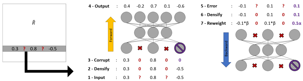
Figure 1: Training steps for auto encoders with incomplete data. The input is drawn from the matrix of ratings, unknown values are turned to zero, some ratings are masked (corruption) and a dense estimate is obtained. Before back propagation, unknown ratings are turned to zero error, prediction errors are reweighted by $\alpha$ and reconstruction errors are reweighted by $\beta$ .

图 1: 不完整数据下自动编码器的训练步骤。输入来自评分矩阵，未知值被置零，部分评分被掩码(破坏)后获得稠密估计。在反向传播前，未知评分的误差被置零，预测误差按 $\alpha$ 重新加权，重构误差按 $\beta$ 重新加权。

First, we inhibit input and output nodes corresponding to missing data. For input nodes, the inhibition is obtained by setting their value to zero. To inhibit the back-propagated unknown errors, we use an empirical loss that disregards the loss of unknown values. No error is back-propagated for missing values, while the error is back-propagated for actual zero values.

首先，我们抑制与缺失数据对应的输入和输出节点。对于输入节点，通过将其值设为零来实现抑制。为了抑制反向传播的未知误差，我们采用了一种经验损失函数，该函数忽略未知值的损失。缺失值不会进行误差反向传播，而实际为零的值则会进行误差反向传播。

where $\widetilde{\mathbf{x}}$ is the corrupted input, $\mathcal{C}$ contains the indices of corrupted elements in $\tilde{\bf x}$ , $\kappa(\mathbf{x})$ contains the indices of known values of $\mathbf{x}$ , W is the flatten vector of weights of the network and $\lambda$ is the regular iz ation parameter. Note that the regular iz ation is applied to the full matrix of weights as opposed to [Sedhain et al., 2015]. The overall training process is described in Fig. 1.

其中 $\widetilde{\mathbf{x}}$ 是受损输入，$\mathcal{C}$ 包含 $\tilde{\bf x}$ 中受损元素的索引，$\kappa(\mathbf{x})$ 包含 $\mathbf{x}$ 已知值的索引，W 是网络权重的展平向量，$\lambda$ 是正则化参数。请注意，与 [Sedhain et al., 2015] 不同，此处正则化应用于完整的权重矩阵。整体训练过程如图 1 所示。

3.2 Integrating Side Information

3.2 整合侧信息

CF only relies on the feedback of the users regarding a set of items. However, adding more information may help to increase the prediction accuracy and robustness. Furthermore, CF suffers from the cold start problem: when little information is available on an item, it will greatly lower the prediction accuracy. We now integrate side information to CFN to alleviate the cold start scenario.

协同过滤 (CF) 仅依赖用户对一组物品的反馈。然而，添加更多信息可能有助于提高预测准确性和鲁棒性。此外，协同过滤存在冷启动问题：当物品信息不足时，会大幅降低预测准确性。我们现在将辅助信息整合到 CFN 中以缓解冷启动场景。

The simplest approach to integrate side information to MF techniques is to append a user/item bias to the rating prediction [Koren et al., 2009]: $\hat{r}{i j}=\mathbf{u}{i}^{T}\mathbf{v}{j}+b_{u,i}+\bar{b_{v,j}}+b^{\prime}$ , where $b_{u,i},b_{v,j},$ $b^{\prime}$ are respectively the user, item, and global bias. These biases are computed with hand-crafted engineering or CF technique [Chen et al., 2012; Porteous et al., 2010; Rendle, 2010]. For instance, side information can directly be concatenated to the feature vector $\mathbf{u}{i}/\mathbf{v}_{j}$ of rank $k$ . Therefore, the estimated rating is computed by:

将辅助信息整合到矩阵分解(MF)技术中最简单的方法是在评分预测中添加用户/物品偏置项 [Koren et al., 2009]：$\hat{r}{i j}=\mathbf{u}{i}^{T}\mathbf{v}{j}+b_{u,i}+\bar{b_{v,j}}+b^{\prime}$，其中 $b_{u,i},b_{v,j},$ $b^{\prime}$ 分别为用户偏置、物品偏置和全局偏置。这些偏置项可通过手工设计或协同过滤(CF)技术计算得出 [Chen et al., 2012; Porteous et al., 2010; Rendle, 2010]。例如，辅助信息可以直接连接到秩为 $k$ 的特征向量 $\mathbf{u}{i}/\mathbf{v}_{j}$ 上。因此，预估评分通过以下公式计算：

$$
\begin{array}{r l}&{\hat{r}{i j}={\mathbf{u}{i},\mathbf{x}{i}}\otimes{\mathbf{v}{j},\mathbf{y}{j}}}\ &{\underline{{\underline{{\mathrm{def}}}}}{[1:k],i}\mathbf{v}{[1:k],j}+\underbrace{\mathbf{x}{i}^{T}\mathbf{v}{[k+1:k+P],j}}{b_{u,i}}+\underbrace{\mathbf{u}{[k+1:k+Q],i}^{T}\mathbf{y}{j}}{b_{v,j}},}\end{array}
$$

$$
\begin{array}{r l}&{\hat{r}{i j}={\mathbf{u}{i},\mathbf{x}{i}}\otimes{\mathbf{v}{j},\mathbf{y}{j}}}\ &{\underline{{\underline{{\mathrm{def}}}}}{[1:k],i}\mathbf{v}{[1:k],j}+\underbrace{\mathbf{x}{i}^{T}\mathbf{v}{[k+1:k+P],j}}{b_{u,i}}+\underbrace{\mathbf{u}{[k+1:k+Q],i}^{T}\mathbf{y}{j}}{b_{v,j}},}\end{array}
$$

where $\mathbf{x}{i}\in\mathbb{R}^{P}$ and $\mathbf{y}_{j}\in\mathbb{R}^{Q}$ encodes user/item side information.

其中 $\mathbf{x}{i}\in\mathbb{R}^{P}$ 和 $\mathbf{y}_{j}\in\mathbb{R}^{Q}$ 编码了用户/物品的辅助信息。

where V′ ∈ R(N×k+P ) is a weight matrix, V[′1:k] ∈ are respectively the submatrices of $\mathbf{V}^{\prime}$ that contain the columns from 1 to $k$ and $k+1$ to $k+P$ . Injecting side information to the last hidden layer as in Eq. 4 enables to partially retrieve the error function of classic hybrid systems described in Eq. 2. Secondly, injecting side information to the other intermediate hidden layers enhance the internal representation. Finally, appending side information to the input vectors supplants the absence of input data when no rating is available. The auto encoder fits CF standards while being trained end-to-end by back propagation.

其中 V′ ∈ R(N×k+P) 是一个权重矩阵，V[′1:k] ∈ 分别是 $\mathbf{V}^{\prime}$ 的子矩阵，包含从 1 到 $k$ 列以及 $k+1$ 到 $k+P$ 列。如公式 4 所示，将辅助信息注入最后一个隐藏层能够部分恢复公式 2 中描述的经典混合系统的误差函数。其次，将辅助信息注入其他中间隐藏层可以增强内部表示。最后，当没有评分数据时，将辅助信息附加到输入向量可以弥补输入数据的缺失。该自编码器符合协同过滤 (CF) 标准，同时通过反向传播进行端到端训练。

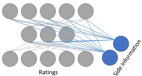
Figure 2: Side information is wired to all the neuron.

图 2: 侧信息连接到所有神经元。

4 Experiments

4 实验

In this section, we empirically evaluate CFN on two major CF datasets: MovieLens and Douban. We first describe the experimental settings before introducing the benchmark models. Finally, we provide an extensive analysis of the results.

在本节中，我们通过两个主流协同过滤(CF)数据集MovieLens和豆瓣对CFN进行实证评估。首先说明实验设置，随后介绍基准模型，最后对结果展开全面分析。

4.1 Experimental Setting

4.1 实验设置

Experiments are conducted on MovieLens and Douban datasets as they are among the biggest CF dataset freely available at the time of writing. Besides, MovieLens contains side information on the items and it is a widespread benchmark while Douban provides side information on the users. The MovieLens-1M, MovieLens-10M and MovieLens-20M respectively provide 1/10/20 million discrete ratings from 6/72/138 thousands users on $4/10/27$ thousands movies. Side information for MovieLens-1M is the age, sex and gender of the user and the movie category (action, thriller etc.). Side information for MovieLens $10/20\mathbf{M}$ is a matrix of tags $\mathbf{T}$ where $T_{i j}$ is the occurrence of the $j^{t h}$ tag for the $i^{t h}$ movie and the movie category. No side information is provided for users. The Douban dataset [Ma et al., 2011] provides 17 million discrete ratings from 129 thousand users on 58 thousands movies. Side information is the bi-directional user/friend relations for the user. The user/friend relations are treated like the matrix of tags from MovieLens. No side information is provided for items. Finally, we perform $90%$ - $10%$ train-test sets as reported in [Lee et al., 2013; Li et al., 2016; Zheng et al., 2016].

实验在MovieLens和豆瓣数据集上进行，因为它们是撰写本文时免费可用的最大协同过滤(CF)数据集之一。此外，MovieLens包含物品的辅助信息且被广泛用作基准，而豆瓣则提供用户的辅助信息。MovieLens-1M、MovieLens-10M和MovieLens-20M分别包含6/72/13.8万用户对$4/10/27$千部电影的100万/1000万/2000万离散评分。MovieLens-1M的辅助信息包括用户年龄、性别和电影类别(动作、惊悚等)。MovieLens $10/20\mathbf{M}$的辅助信息是标签矩阵$\mathbf{T}$，其中$T_{i j}$表示第$i$部电影第$j$个标签的出现次数及电影类别。未提供用户辅助信息。豆瓣数据集[Ma et al., 2011]包含12.9万用户对5.8万部电影的1700万离散评分。辅助信息是用户间的双向好友关系，其处理方式与MovieLens的标签矩阵相同。未提供物品辅助信息。最终，我们按照[Lee et al., 2013; Li et al., 2016; Zheng et al., 2016]报告的方法，采用$90%$-$10%$的训练集-测试集划分。

Preprocessing For each dataset, we first centered the ratings to zero-mean by row (resp. by col) for U-CFN (resp I-CFN): denoting $b_{i}$ the mean of the $\dot{i}^{t h}$ user and $b_{j}$ the mean of the $j^{t h}$ item, U-CFN and I-CFN respectively learn from $r_{i j.}^{u n b i a s e d}=r_{i j}-b_{i}$ and $r_{i j}^{u n b i a s e d}=\bar{r_{i j}}-b_{j}$ . Then all the ratings are linearly rescaled from $^{-1}$ to 1 to fit the output range of the auto encoder transfer functions. Theses operations are finally reversed while evaluating the final matrix.

预处理
对于每个数据集，我们首先通过行（对应U-CFN）或列（对应I-CFN）将评分中心化为零均值：设$b_{i}$为用户$\dot{i}^{t h}$的均值，$b_{j}$为物品$j^{t h}$的均值，U-CFN和I-CFN分别从$r_{i j.}^{u n b i a s e d}=r_{i j}-b_{i}$和$r_{i j}^{u n b i a s e d}=\bar{r_{i j}}-b_{j}$中学习。随后，所有评分被线性缩放至$^{-1}$到1之间，以适应自动编码器传递函数的输出范围。最终在评估矩阵时，这些操作会被逆向还原。

Side Information As the dimensionality of the side information is huge, we first perform a dimension reduction of the matrix of tags/friendships. To do so, we use a low rank matrix factorization in our experiments. For a different nature of data as texts or pictures (which are not available in our dataset), CFN can directly learn this embedding as [Wang and Wang, 2014; Wang et al., 2014; Li et al., 2015]. Formally, we use the left part of a matrix factorization of the tag matrix $\mathbf{T}$ . From $\mathbf{T}=\mathbf{\dot{P}D Q}^{T}$ with $\mathbf{D}$ tthhee d miao g vio en taal gms aatrrie xr eofp ree is gee n nt ve adl ubeys ${\bf Y}={\bf P}{J\times K^{\prime}}{\bf D}_{K^{\prime}\times K^{\prime}}^{0.5}$ o rwdietrh, the number of kept ei gen vectors. Binary representation such as the movie category is concatenated to $\mathbf{Y}$ .

辅助信息
由于辅助信息的维度极高，我们首先对标签/好友关系矩阵进行降维处理。实验采用低秩矩阵分解方法实现降维。对于文本或图片等不同性质的数据（本数据集未包含），CFN可直接学习嵌入表示[Wang and Wang, 2014; Wang et al., 2014; Li et al., 2015]。具体实现上，我们使用标签矩阵$\mathbf{T}$的矩阵分解左半部分：由$\mathbf{T}=\mathbf{\dot{P}DQ}^{T}$（其中$\mathbf{D}$为对角特征值矩阵）得到降维表示${\bf Y}={\bf P}{J\times K^{\prime}}{\bf D}_{K^{\prime}\times K^{\prime}}^{0.5}$，此处$K^{\prime}$为保留的特征向量数量。电影类别等二元表征信息将与$\mathbf{Y}$进行拼接。

Error Function The algorithms are compared based on their respective Root Mean Square Error (RMSE) on test data. Denoting $\mathbf{R}^{\mathbf{test}}$ the matrix of test ratings and $\widehat{\mathbf{R}}$ the full matrix returned by the learning algorithm, the RM bSE is:

误差函数
算法基于它们在测试数据上的均方根误差 (Root Mean Square Error, RMSE) 进行比较。设 $\mathbf{R}^{\mathbf{test}}$ 为测试评分矩阵，$\widehat{\mathbf{R}}$ 为学习算法返回的完整矩阵，则 RMSE 为：

$$
L(\widehat{\bf R},{\bf R}^{\sf t e s t})=\sqrt{\frac{1}{|K(R^{t e s t})|}\sum_{(i,j)\in{\cal K}(R^{t e s t})}(r_{i j}^{t e s t}-\hat{r}_{i j})^{2}},
$$

$$
L(\widehat{\bf R},{\bf R}^{\sf t e s t})=\sqrt{\frac{1}{|K(R^{t e s t})|}\sum_{(i,j)\in{\cal K}(R^{t e s t})}(r_{i j}^{t e s t}-\hat{r}_{i j})^{2}},
$$

where $|K(R^{t e s t})|$ is the number of ratings in the testing dataset. Note that in the case of auto encoders $\widehat{\mathbf{R}}$ is computed by feeding the network with training data. As sbuch, $\hat{r}{i j}$ stands for $n n(\hat{\mathbf{r}}{\mathbf{i},.}^{t r a i n}){j}$ for U-CFN, and $n n(\hat{\mathbf{r}}{\mathbf{\alpha}\mathbf{\cdot}\mathbf{j}}^{t r a i n})_{i}$ for I-CFN.

其中 $|K(R^{test})|$ 是测试数据集中的评分数量。需要注意的是，对于自编码器 (auto encoders) ，$\widehat{\mathbf{R}}$ 是通过向网络输入训练数据计算得出的。因此，$\hat{r}{ij}$ 在 U-CFN 中表示 $nn(\hat{\mathbf{r}}{\mathbf{i},.}^{train}){j}$，在 I-CFN 中表示 $nn(\hat{\mathbf{r}}{\mathbf{\alpha}\mathbf{\cdot}\mathbf{j}}^{train})_{i}$。

Training Settings We train a one-hidden layer autoencoders with hyperbolic tangent transfer functions. The layers have 600 hidden neurons. Weights are randomly initialized with a uniform law $\mathbf{W_{ij}}\sim\mathcal{U}\bar{[-1/\sqrt{n},1/\sqrt{n}]}$ . The latent dimension of the low rank matrix of tags/friendships is set to 50. Hyper param enters were are fine-tuned by a genetic algorithm and the final learning rate, learning decay and weight decay are respectively set to 0.7, 0.3 and 0.5. α, $\beta$ and masking ratio are set to 1, 0.5 and 0.25.

训练设置
我们训练了一个带有双曲正切传递函数的单隐藏层自编码器。该网络层包含600个隐藏神经元。权重采用均匀分布随机初始化：$\mathbf{W_{ij}}\sim\mathcal{U}\bar{[-1/\sqrt{n},1/\sqrt{n}]}$。标签/好友关系的低秩矩阵潜在维度设置为50。超参数通过遗传算法进行微调，最终学习率、学习衰减率和权重衰减率分别设为0.7、0.3和0.5。α、$\beta$和掩码比例分别设置为1、0.5和0.25。

Source code In order to ensure easy reproducibility and reuse the experimental results, we provide the code in an outof-the-box tutorial in Torch. 1.

源代码
为确保实验结果的易复现性和可重用性，我们以开箱即用教程形式提供基于 Torch 的代码实现。

4.2 Benchmark Models

4.2 基准模型

We benchmark CFN with five matrix completion algorithms:

我们使用五种矩阵补全算法对CFN进行基准测试：

• ALS-WR (Alternating Least Squares with Weighted $\cdot\lambda$ - Regular iz ation) [Zhou et al., 2008] solves the low-rank MF problem by alternatively fixing U and V and solving the resulting linear regression problem. Experiments are run with the Apache Mahout Software 2 with a rank of 200; SVDFeature [Chen et al., 2012] learns a feature-based MF : side information is used to predict the bias term and to reweight the matrix factorization. We use a rank of 64 and tune other hyper parameters by random search; BPMF (Bayesian Probabilistic Matrix Factorization) infers the matrix decomposition after a statistical model.

• ALS-WR (带加权$\cdot\lambda$正则化的交替最小二乘法) [Zhou et al., 2008] 通过交替固定U和V并求解所得线性回归问题来解决低秩矩阵分解问题。实验使用Apache Mahout Software 2运行，秩为200；
• SVDFeature [Chen et al., 2012] 学习基于特征的矩阵分解：利用辅助信息预测偏置项并重新加权矩阵分解。我们使用秩为64的分解，并通过随机搜索调整其他超参数；
• BPMF (贝叶斯概率矩阵分解) 在统计模型后推断矩阵分解。

Table 1: RMSE on MovieLens-10M $(90%/10%)$ ). The $^{++}$ suffix denotes when side information is added to CFN.

算法	MovieLens-1M	MovieLens-10M	MovieLens-20M	Douban
BPMF	0.8705±4.3e-3	0.8213±6.5e-4	0.8123±3.5e-4	0.7133±3.0e-4
ALS-WR	0.8433±1.8e-3	0.7830±1.9e-4	0.7746±2.7e-4	0.7010±3.2e-4
SVDFeature	0.8631±2.5e-3	0.7907±8.4e-4	0.7852±5.4e-4	*
LLORMA	0.8371±2.4e-3	0.7949±2.3e-4	0.7843±3.2e-4	0.6968±2.7e-4
I-Autorec	0.8305±2.8e-3	0.7831±2.4e-4	0.7742±4.4e-4	0.6945±3.1e-4
U-CFN	0.8574±2.4e-3	0.7954±7.4e-4	0.7856±1.4e-4	0.7049±2.2e-4
U-CFN++	0.8572±1.6e-3	N/A	N/A	0.7050±1.2e-4
I-CFN	0.8321±2.5e-3	0.7767±5.4e-4	0.7663±2.9e-4	0.6911±3.2e-4
I-CFN++	0.8316±1.9e-3	0.7754±6.3e-4	0.7652±2.3e-4	N/A

表 1: MovieLens-10M上的RMSE (90%/10%)。$^{++}$后缀表示向CFN添加了辅助信息。

As a bayesian algorithm, the performances can be improved by the fine tuning of priors over the parameters Here, we use the recommendations of [Salak hut dino v and Mnih, 2008] for priors and rank (set to 10).

作为一种贝叶斯算法，通过微调参数先验可以提升性能。这里我们采用 [Salakhutdinov 和 Mnih, 2008] 推荐的先验设置和秩值 (设为 10)。

LLORMA estimates the rating matrix as a weighted sum of low-rank matrices. Experiments are run with the Prea API3. We use a rank of 20, 30 anchor points which entail a global pseudo-rank of 600. Other hyper para meters are picked as recommended in [Lee et al., 2013]; I-Autorec [Sedhain et al., 2015] trains one auto encoder per item, sharing the weights between the different autoencoders. We use 600 hidden neurons with the training hyper parameters recommended by the author.

LLORMA将评分矩阵估计为多个低秩矩阵的加权和。实验通过Prea API3运行，采用秩为20、30个锚点的设置，对应全局伪秩为600。其余超参数按照[Lee et al., 2013]的建议选取；I-Autorec [Sedhain et al., 2015]为每个物品训练一个自编码器，并在不同自编码器间共享权重。我们使用600个隐藏神经元，训练超参数遵循原作者推荐值。

In every scenario, we select the highest possible rank which does not lead to over fitting despite a strong regular iz ation. For instance, increasing the rank of BPMF does not significantly increase the final RMSE, idem for SVDFeature. Similar benchmarks exist in the literature [Lee et al., 2013; Li et al., 2016; Zheng et al., 2016].

在每种情况下，我们都选择不会导致过拟合的最高可能秩 (rank) ，尽管进行了强正则化。例如，增加 BPMF 的秩不会显著提高最终 RMSE，SVDFeature 也是如此。文献中存在类似的基准测试 [Lee et al., 2013; Li et al., 2016; Zheng et al., 2016]。

4.3 General Results

4.3 通用结果

Comparison to state-of-the-art Tab. 1 summarizes the RMSE on MovieLens and Douban datasets. Confidence intervals correspond to a $95%$ range. I-CFNs have excellent performance for every dataset we run. It is competitive compared to the state-of-the-art CF algorithms and outperforms them for MovieLens-10M. To the best of our knowledge, the best result published for MovieLens-10M (without side information) has a final RMSE of 0.7682 [Li et al., 2016]. Note that I-CFN outperforms U-CFN as shown in Fig. 5. It suggests that the structure of the items is stronger than the one on the users i.e. it is easier to guess tastes based on movies you liked than to find users similar to you. Yet, this behavior could be different on another dataset. Finally, I-CFN outperforms Autorec on big dataset while both methods rely on auto encoder. In addition to the DAE loss, CFN benefits from regularizing missing ratings during the training as described in Eq. 1. Thus, uncommon ratings are more regularized and they turn out to be less overfitted.

与现有最优技术的对比
表 1 总结了 MovieLens 和 Douban 数据集上的均方根误差 (RMSE)。置信区间对应 95% 范围。I-CFN 在我们运行的每个数据集中都表现出色。相较于现有最优的协同过滤 (CF) 算法，它具有竞争力，并在 MovieLens-10M 数据集上表现更优。据我们所知，MovieLens-10M (无辅助信息) 已发布的最佳结果为 0.7682 [Li et al., 2016]。值得注意的是，如图 5 所示，I-CFN 优于 U-CFN。这表明物品的结构性比用户更强，即基于喜欢的电影猜测品味比寻找相似用户更容易。然而，这种行为在其他数据集上可能不同。最后，在大型数据集上，I-CFN 优于 Autorec，尽管两种方法都依赖于自动编码器。除了 DAE 损失外，CFN 还受益于训练期间对缺失评分的正则化 (如公式 1 所述)。因此，罕见评分的正则化更强，过拟合程度更低。

Impact of side information At first sight at Tab. 1, the use of side information has a limited impact on the RMSE. This statement has to be mitigated: as the re partition of known entries in the dataset is not uniform, the estimates are biased towards users and items with a lot of ratings. For theses users and movies, the dataset already contains a lot of information, thus having some extra information will have a marginal effect. Users and items with few ratings should benefit more from some side information but the estimation bias hides them. In order to exhibit the utility of side information, we report in Tab. 2 the RMSE conditionally to the number of missing values for items. As expected, the fewer number of ratings for an item, the more important is the side information. This is very desirable for a real system: the effective use of side information to the new items is crucial to deal with the flow of new products. A more careful analysis of the RMSE improvement in this setting shows that the improvement is uniformly distributed over the users whatever their number of ratings. This corresponds to the fact that the available side information is only about items. Finally, we train I-CFN on MovieLens-10M $(90%/10%)$ with either the movie genre or the matrix of tags. Individually picked, side information increases the global RMSE by $0.10%$ while concatenating them increases the final score by $0.14%$ . Therefore, I-CFN handles the heterogeneity of side information.

侧信息的影响
初看表1时，侧信息的使用对RMSE（均方根误差）的影响有限。这一结论需要修正：由于数据集中已知条目的分布不均匀，估计结果会偏向于拥有大量评分的用户和项目。对这些用户和电影而言，数据集中已包含大量信息，因此额外的侧信息只会产生边际效应。评分较少的用户和项目本应从侧信息中获益更多，但估计偏差掩盖了这一点。

为了展示侧信息的效用，我们在表2中按项目缺失值的数量条件性地报告了RMSE。正如预期，项目的评分数量越少，侧信息的作用就越重要。这对实际系统非常有利：有效利用新项目的侧信息对于处理新产品流至关重要。

更细致的RMSE改进分析表明，在此设置下，改进均匀分布在用户之间，无论他们的评分数量如何。这与可用侧信息仅涉及项目的事实相符。

最后，我们在MovieLens-10M数据集 $(90%/10%)$ 上训练I-CFN，分别使用电影类型或标签矩阵作为侧信息。单独选取时，侧信息使全局RMSE提升 $0.10%$，而将它们拼接后，最终得分提升 $0.14%$。因此，I-CFN能够处理侧信息的异构性。

Figure 3: Impact of the denoising loss in the training process. $\alpha=1$ is kept constant while varying the reconstruction hyper parameter $\beta$ and the masking ratio .

图 3: 去噪损失在训练过程中的影响。保持 $\alpha=1$ 不变，同时调整重建超参数 $\beta$ 和掩码比例。

Impact of the loss The DAE loss positively impacts the final RMSE on big dataset as highlighted in Fig. 3 when carefully balanced. Surprisingly, the auto encoder has already good generalization properties while only focusing on the reconstruction criterion (no masking). More importantly, the reconstruction criterion cannot be discarded ( $\beta=0,$ ) to learn an efficient representation.

损失函数的影响
如图3所示，当DAE（去噪自编码器）损失函数经过仔细平衡后，能显著提升大型数据集上的最终RMSE（均方根误差）。令人惊讶的是，即使仅聚焦于重构标准（无掩码处理），自编码器已展现出良好的泛化特性。更重要的是，若完全舍弃重构标准（$\beta=0$），将无法学习到有效的表征。

Figure 4: RMSE vs training set ratio for MovieLens-10M. Training hyperparameters are kept constant across dataset. CFN and I-Autorec are very robust to a change in the density while SVDFeature must be refined each time.

图 4: MovieLens-10M数据集上RMSE随训练集比例的变化。所有训练超参数在数据集间保持恒定。CFN和I-Autorec对数据密度变化表现出很强鲁棒性，而SVDFeature每次都需要重新调参。

Table 2: RMSE computed by clusters of items sorted by the number of ratings on MovieLens-10M $(90%/10%)$ . For instance, the first cluster contains the $20%$ of items with the lowest number of ratings.

(b) MovieLens-10M $90%/10%$ )

表 2: 按 MovieLens-10M 中评分数量排序的物品集群计算的 RMSE $(90%/10%)$ 。例如，第一个集群包含评分数量最低的 $20%$ 物品。

Interval	I-CFN	I-CFN++ %Improv.
0.0-0.2	1.0030	0.9938 0.96
0.2-0.4	0.9188	0.9084 1.15
0.4-0.6	0.8748	0.8669 0.91
0.6-0.8	0.8473	0.8420 0.63
0.8-1.0	0.7976	0.7964 0.15
Full	0.8075	0.8055 0.25

(a) MovieLens-10M (50%/50%)

Interval	I-CFN	I-CFN++ %Improv.
0.0-0.2	0.9539	0.9444 1.01
0.2-0.4	0.8815	0.8730 0.96
0.4-0.6	0.8487	0.8408 0.95
0.6-0.8	0.8139	0.8110 0.35

(b) MovieLens-10M $(90%/10%)$

Impact of the non-linearity We removed the non-linearity from I-CFN to study its relative impact. For fairness, we kept $\alpha,\beta$ , the masking ratio and the number of hidden neurons constant. We fine-tune the learning rates and weight decay. For MovieLens-10M, we obtain a final RMSE of $0.8151\pm$ 1.4e-3 which is far worse than classic non-linear I-CFN.

非线性影响研究
我们移除了I-CFN中的非线性结构以评估其相对影响。为保证公平性，保持参数$\alpha,\beta$、掩码比例及隐藏神经元数量不变，仅微调学习率和权重衰减率。在MovieLens-10M数据集上，最终RMSE为$0.8151\pm$1.4e-3，显著劣于经典非线性I-CFN模型。

Impact of the training ratio CFN remains very robust to a variation of data density as shown in Fig. 4. It is all the more impressive that hyper parameters are first optimized for movieLens-10M $(90%/10%)$ ). Cold-start and warm-start scenario are also far more well-handled by NNs than more classic CF algorithms.

训练比例的影响
如图 4 所示，CFN (Collaborative Filtering Network) 对数据密度的变化表现出极强的鲁棒性。更令人印象深刻的是，超参数最初是为 MovieLens-10M $(90%/10%)$ 优化的。与传统的协同过滤算法相比，神经网络在冷启动和热启动场景中的表现也更为出色。

4.4 CFN Tract ability

4.4 CFN可处理性

One major problem faced by CF algorithms is s cal ability as CF datasets contain hundred of thousands of users and items.

协同过滤 (CF) 算法面临的一个主要问题是可扩展性，因为 CF 数据集包含数十万用户和物品。

Figure 5: RMSE by epoch for CFN for MovieLens-10M $(90%/10%)$ ).

图 5: MovieLens-10M数据集上CFN模型各epoch的RMSE值 (90%/10%)

Table 3: Training time and memory footprint for a 2-layers CFN on GTX 980 for 20 epochs.

表 3: GTX 980 上训练 2 层 CFN 20 个周期的耗时与内存占用

模型	数据集	参数量	耗时	内存占用
U-CFN	MLens-1M	5M	7m17s	262MiB
	MLens-10M	15M	34m51s	543MiB
	MLens-20M	38M	59m35s	1,044MiB
I-CFN	MLens-1M	8M	2m03s	250MiB
	MLens-10M	100M	18m34s	1,532MiB
	MLens-20M	194M	34m45s	2,905MiB

Recent advances in GPU computation managed to reduce the training time of NNs by several orders of magnitude. CFN (and ALS-WR) fully benefits from those advances and is trained within a few minutes as shown in Tab. 3. On the other side, CF gradient based methods such as SVDFeature [Chen et al., 2012] cannot be easily parallel i zed or used on GPU as they are mainly iterative. Similarly, Autorec [Sedhain et al., 2015] suffers from synchronization and memory fetching latencies because of the shared weights among auto encoders. Furthermore, CFN has the key advantage to provide excellent performance while being able to refine its prediction on the fly for new ratings. Thus, U-CFN/I-CFN does not need to be retrained for new items/users.

GPU计算的最新进展成功将神经网络(NN)的训练时间缩短了几个数量级。如表3所示，CFN(以及ALS-WR)充分受益于这些进展，仅需几分钟即可完成训练。另一方面，基于CF梯度的方法(如SVDFeature [Chen et al., 2012])由于主要是迭代式的，难以并行化或应用于GPU。同样地，Autorec [Sedhain et al., 2015]因自编码器间共享权重而面临同步和内存获取延迟问题。此外，CFN具有关键优势：既能提供卓越性能，又能实时根据新评分动态优化预测。因此，U-CFN/I-CFN无需针对新用户/物品进行重新训练。

5 Conclusion

5 结论

In this paper, we highlight the connections between autoencoders and matrix factorization for matrix completion. We pack some modern training techniques - as well than some code - able to defeat state of the art methods while remaining scalable. Moreover, we propose a systematic way to integrate side information without the need to combine two separate systems. To some extent, this work extends the construction of embeddings by neural networks to the collaborative filtering setting. A natural follow-up is to work with deeper archi tec ture s using batch normalization [Sergey and Szegedy, 2015], adaptive gradient methods (such as ADAM [Kingma and Ba, 2014]) or residual networks [He et al., 2015]. Other extensions could use recurrent networks to grasp the sequential aspect of the collection of ratings.

本文重点探讨了自编码器与矩阵分解在矩阵补全任务中的关联性。我们整合了若干现代训练技术及代码实现，在保持可扩展性的同时超越了现有最优方法。此外，我们提出了一种系统性整合辅助信息的方案，无需依赖两个独立系统的组合。这项工作在某种程度上将神经网络构建嵌入向量的方法扩展到了协同过滤场景。后续研究可自然延伸至采用批归一化 [Sergey and Szegedy, 2015]、自适应梯度方法（如ADAM [Kingma and Ba, 2014]）或残差网络 [He et al., 2015] 的深层架构。其他扩展方向包括利用循环网络捕捉评分序列的时序特性。