CLRerNet: Improving Confidence of Lane Detection with LaneIoU
CLRerNet: 基于 LaneIoU 提升车道线检测置信度
Abstract
摘要
Lane marker detection is a crucial component of the autonomous driving and driver assistance systems. Modern deep lane detection methods with row-based lane represent ation exhibit excellent performance on lane detection benchmarks. Through preliminary oracle experiments, we firstly disentangle the lane representation components to determine the direction of our approach. We show that correct lane positions are already among the predictions of an existing row-based detector, and the confidence scores that accurately represent intersection-overunion (IoU) with ground truths are the most beneficial. Based on the finding, we propose LaneIoU that better correlates with the metric, by taking the local lane angles into consideration. We develop a novel detector coined CLRerNet featuring LaneIoU for the target assignment cost and loss functions aiming at the improved quality of confidence scores. Through careful and fair benchmark including cross validation, we demonstrate that CLRerNet outperforms the state-of-the-art by a large margin - enjoying F1 score of $8l.43%$ compared with $80.47%$ of the existing method on CULane, and $86.47%$ compared with $86.I O%$ on CurveLanes. Code and models are available at https: //github.com/hiroto musik er/CLRerNet.
车道线检测是自动驾驶和驾驶员辅助系统的关键组成部分。采用基于行的车道表示方法的现代深度车道检测技术在车道检测基准测试中表现出卓越性能。通过初步实验验证,我们首先解构了车道表示组件以确定研究方向。研究表明,现有基于行的检测器预测结果中已包含正确的车道位置,而能准确反映预测与真实值交并比(IoU)的置信度分数最具价值。基于这一发现,我们提出LaneIoU方法,通过考虑局部车道角度使其与评估指标更相关。我们开发了新型检测器CLRerNet,其采用LaneIoU作为目标分配代价和损失函数,旨在提升置信度评分质量。经过包含交叉验证在内的严谨公平测试,证明CLRerNet大幅超越现有最优技术——在CULane数据集上F1分数达81.43%(对比现有方法的80.47%),在CurveLanes数据集上达86.47%(对比86.10%)。代码与模型详见https://github.com/hirotomusiker/CLRerNet。
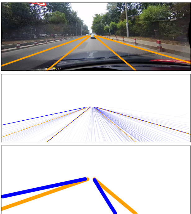
Figure 1: Lane detection example. top: ground truth. middle: all the predictions (blue, deeper for higher confidence scores) and ground truths (dashed orange). bottom: metric IoU calculation by comparing segmentation masks of predictions (blue) and GTs (orange). Best viewed in color.
图 1: 车道线检测示例。上:真实标注。中:所有预测结果(蓝色,颜色越深表示置信度分数越高)和真实标注(橙色虚线)。下:通过比较预测分割掩膜(蓝色)与真实标注(橙色)计算IoU指标。建议彩色查看。
1. Introduction
1. 引言
Lane (marker) detection plays an important role in the autonomous driving and driver assistance systems. Like other computer vision tasks, emergence of convolutional neural networks (CNNs) has brought rapid progress on lane detection performance. Modern lane detection methods are grouped into four categories in terms of lane instance representation. Segmentation-based [18, 27] and keypoint-based [21] representations regard lanes as segmentation mask and keypoints respectively. The parametric representation methods [25, 16] utilize curve parameters to regress lane shapes. The row-based representation [24, 28, 19, 20, 15] regards a lane as a set of coordinates on the certain horizontal lines. The first two representations are employed in the bottom-up detection paradigm, where the lane positions are directly detected in the image and grouped into lane instances afterwards. The latter two are adopted to the top-down instance detection methods where each lane detection is regarded as both global lane instance and a set of local lane points. The row-based representation is the defacto standard in terms of detection performance among the above representation types. We choose the best-performing CLRNet [28] from the row-based methods as our baseline.
车道线检测在自动驾驶和驾驶辅助系统中扮演着重要角色。与其他计算机视觉任务类似,卷积神经网络(CNN)的出现推动了车道检测性能的快速提升。现代车道检测方法根据车道实例表示形式可分为四类:基于分割[18, 27]和基于关键点[21]的方法分别将车道视为分割掩膜和关键点;参数化表示方法[25, 16]通过曲线参数回归车道形状;基于行的表示方法[24, 28, 19, 20, 15]将车道视为特定水平线上的一组坐标点。前两种表示属于自底向上的检测范式,即先在图像中直接检测车道位置再组合成车道实例;后两种则用于自顶向下的实例检测方法,将每条车道检测视为全局车道实例与局部车道点的集合。在上述表示类型中,基于行的表示是检测性能的事实标准。我们从基于行的方法中选择了性能最优的CLRNet[28]作为基线模型。
The performance of lane detection relies on lane point localization and instance-wise classification. The lane detection benchmarks [18, 7] employ segmentation-maskbased intersection-over-union (IoU) between predicted and ground-truth (GT) lanes as an evaluation metric. The predicted lanes whose scores are above the predefined threshold are treated as valid predictions to calculate F1 score. Therefore, the predicted lanes with large segmentationbased IoUs with GTs should have large classification scores.
车道检测的性能依赖于车道点定位和实例级分类。车道检测基准[18, 7]采用预测车道与真实标注(GT)车道之间基于分割掩码的交并比(IoU)作为评估指标。得分超过预设阈值的预测车道被视为有效预测以计算F1分数。因此,与GT具有较大基于分割IoU的预测车道应具有较高的分类分数。
To determine the direction of our approach, we firstly conduct the preliminary oracle experiments h by replacing the confidence score, anchor parameters and length of each prediction with the oracle values. By making the confidence scores oracle, the F1 score goes to near-perfect $98.47%$ . The result implies the correct lanes are already among the predictions, however the confidence scores need to be predicted accurately representing the metric IoU. Fig. 1 (middle) shows the comparison between all the predictions (blue) and GTs (dashed orange). The color depth of the predictions is proportional to their confidence scores. The left-most prediction is the high-confidence false positive that misses the ground truth, however there is a correct low-confidence prediction near the GT which has a high IoU.
为了确定我们的方法方向,我们首先进行了初步的理想实验,通过将每个预测的置信度分数、锚点参数和长度替换为理想值。当置信度分数设为理想值时,F1分数接近完美值 $98.47%$ 。结果表明正确的车道线已存在于预测结果中,但需要准确预测反映IoU指标的置信度分数。图1(中)展示了所有预测(蓝色)与真实值(虚线橙色)的对比。预测线条的颜色深度与其置信度分数成正比。最左侧的预测是一个高置信度的假阳性结果,未能匹配真实值,但在真实值附近存在一个IoU较高的低置信度正确预测。
The next question is: how could the segmentation-based IoU be implemented as a learning target? In the row-based methods, the prediction and GT lanes are both represented as sets of $x$ coordinates at the fixed rows. [28] introduces the LineIoU loss to measure the intersection and union row by row and sum them up respectively. However, this approach is not equivalent to the segmentation-based IoU especially for the non-vertical, tilted lanes (e.g. Fig. 1 bottom) or curves. We introduce the novel IoU coined LaneIoU, which takes local lane angles of the lanes into account. The LaneIoU integrates the angle-aware intersection and union of each row to match the segmentation-based IoU.
接下来的问题是:如何将基于分割的交并比(IoU)实现为学习目标?在基于行的方法中,预测车道线和真实车道线都被表示为固定行上的一组$x$坐标。[28]提出了LineIoU损失函数,通过逐行计算交集和并集并分别求和来度量。然而,这种方法并不等同于基于分割的交并比,特别是对于非垂直的倾斜车道线(例如图1底部)或曲线。我们提出了新颖的LaneIoU,它考虑了车道线的局部角度。LaneIoU通过整合每行角度感知的交集和并集,来匹配基于分割的交并比。
The row-based methods learn global lane probability scores for each anchor. The dynamic sample assignment employed in the recent object detector [4, 5] is also effective for lane detection training [28]. The IoU matrix and the cost matrix between the predicted lanes and the GTs respectively determine the number of anchors to assign for each GT and which anchors to assign. The confidence targets of the assigned anchors are set to positive (one). Therefore, sample assignment is responsible for learning the confidence scores. We introduce LaneIoU to sample assignment in order to bring the detector’s confidence scores close to the segmentation-based IoU. LaneIoU dynamically determines the number of anchors to assign and prioritizes the anchors to assign as a cost function. Moreover, the loU loss to regress the horizontal coordinates is also replaced by our LaneIoU to appropriately penalize the predicted lanes at different tilt angles. The LaneIoU integration to CLRNet [28] makes the detector’s training more straightforward, thus we coin our method CLRerNet.
基于行的方法为每个锚点学习全局车道概率分数。近期目标检测器[4,5]采用的动态样本分配策略在车道检测训练中同样有效[28]。预测车道与真实标注(GT)之间的IoU矩阵和成本矩阵分别决定了为每个GT分配的锚点数量及具体分配方案。被分配锚点的置信度目标设为正值(1)。因此样本分配机制负责学习置信度分数。我们引入LaneIoU到样本分配中,使检测器的置信度分数更接近基于分割的IoU。LaneIoU动态决定待分配锚点数量,并作为成本函数优先分配特定锚点。此外,回归水平坐标的IoU损失也被替换为LaneIoU,以针对不同倾斜角度的预测车道施加合理惩罚。将LaneIoU集成到CLRNet[28]后,检测器训练过程更加直观,因此我们将该方法命名为CLRerNet。
We showcase the effectiveness of LaneIoU through extensive experiments on CULane and CurveLanes and report the state-of-the-art results on both datasets. Importantly, for a reliable and fair benchmark, we employ the average score of five models for each experiment condition, while prior work shows a score of a single model. Moreover, the F1 metric employed in the lane detection evaluation is utterly sensitive to the detector’s lane confidence threshold, thus we determine the threshold utilizing the 5-fold cross validation on the train split.
我们通过在CULane和CurveLanes数据集上的大量实验展示了LaneIoU的有效性,并报告了这两个数据集上的最先进结果。值得注意的是,为确保基准测试的可靠性和公平性,我们对每个实验条件采用五个模型的平均分数,而先前工作仅展示单一模型的分数。此外,车道检测评估中采用的F1指标对检测器的车道置信度阈值极为敏感,因此我们通过在训练集上使用5折交叉验证来确定该阈值。
Our contributions in this paper are threefold:
我们在本文中的贡献有三方面:
2. Related Work
2. 相关工作
2.1. Object detection
2.1. 目标检测
Training sample assignment. Sample assignment is the major research focus in object detection. The proposals from the detection head are assigned to the ground truth samples. [22, 13, 8, 12] assign the GTs by calculating IoU between the anchors on the feature map grid and GT boxes statically. [4] introduces the optimal transfer assignment (OTA) for object detector’s training sample assignment, that dynamically assigns the prediction boxes to the GTs. [5] simplifies OTA and realizes iteration-free assignment.
训练样本分配。样本分配是目标检测的主要研究方向。检测头生成的候选框会被分配给真实样本。[22, 13, 8, 12] 通过静态计算特征图网格上锚框与真实框的交并比(IoU)进行分配。[4] 提出了目标检测器训练样本分配的最优传输分配(OTA)方法,动态地将预测框分配给真实框。[5] 简化了OTA并实现了无需迭代的分配方案。
IoU functions. Several variants of IoU functions [23, 29, 30] are proposed for accurate bounding box regression and fast convergence. For example, the generalized IoU (GIoU) [23] introduces the smallest convex hull of the boxes and makes IoU differentiable even when the bounding boxes do not overlap. Our LaneIoU is based on GIoU but newly enables the IoU calculation between curves in the row-based representation.
IoU函数。为了精确的边界框回归和快速收敛,研究者们提出了多种IoU函数的变体[23, 29, 30]。例如,广义IoU (GIoU) [23]引入了边界框的最小凸包,使得即使边界框不重叠时IoU也可微分。我们的LaneIoU基于GIoU,但创新性地实现了基于行表示法(curve)的曲线间IoU计算。
2.2. Lane detection
2.2. 车道检测
Lane detection paradigms are grouped by lane representation types, namely segmentation-based, keypoint-based, row-based and parametric representations.
车道检测范式按车道表示类型分组,包括基于分割 (segmentation-based) 、基于关键点 (keypoint-based) 、基于行 (row-based) 和参数化表示 (parametric representations) 。
Segmentation-based representation. This line of work is the bottom-up pixel-based estimation of lane existence probability. SCNN [18] and RESA [27] employ a semantic segmentation paradigm to classify the lane instances as separate classes on each pixel. The correspondence between lane and class is determined by annotation thus not flexible (e.g. some lane position may belong to two classes). The benchmark datasets [18, 7] employ pixel-level IoU to compare predicted lanes with GTs, and are friendly to the segmentation-based methods. However the methods do not treat lanes as holistic instances and require post-processing which is computationally costly. [19, 28] exploit the segmentation task as the auxiliary loss only during training time to improve the backbone network. We follow these methods and adopt the auxiliary branch and loss.
基于分割的表征方法。这类工作采用自底向上的像素级概率估计来预测车道线存在概率。SCNN [18] 和 RESA [27] 使用语义分割范式,将每个像素上的车道实例分类为不同类别。车道线与类别的对应关系由标注决定,因此缺乏灵活性(例如某些车道位置可能同时属于两个类别)。基准数据集 [18, 7] 采用像素级 IoU 来比较预测车道线与真实标注,这对基于分割的方法较为友好。但这类方法未将车道线视为整体实例,且需要耗时的后处理流程。[19, 28] 仅在训练阶段将分割任务作为辅助损失函数来提升主干网络性能。我们沿用这些方法,采用辅助分支和损失函数。
Keypoint-based representation. Similar to human pose estimation, the lane points are detected as keypoints and grouped into lane instances afterwards. PINet [11] employs test-time detachable stacked hourglass networks to learn keypoint probabilities and cluster the keypoints into the lane instances. FOLOLane [21] also detects lanes as keypoints inspired by the bottom-up human pose detection method [1]. GANet [10] regresses the offsets of the detected keypoints from the starting point of the corresponding lane instances. This line of methods requires post-process to group the lane points into lane instances, which is computationally expensive.
基于关键点的表示。与人体姿态估计类似,车道点被检测为关键点,随后分组为车道实例。PINet [11] 采用可拆卸的堆叠沙漏网络在测试时学习关键点概率,并将关键点聚类为车道实例。FOLOLane [21] 也受自底向上人体姿态检测方法 [1] 启发,将车道检测为关键点。GANet [10] 通过回归检测到的关键点相对于对应车道实例起点的偏移量来预测车道。这类方法需要后处理将车道点分组为车道实例,计算成本较高。
Parametric representation. In this line of work, a lane instance is represented as a set of curve parameters. Poly Lane Net [25] employs a curve representation using polynomial coefficients. LSTR [16] employs end-to-end transformer-based lane parameter set detection. BSNet [2] chooses the quasi-uniform b-spline curves and shows the highest F1 score among this category. These methods achieve relatively fast inference, however an error of one parameter holistic ally affects the lane shape.
参数化表示。在这类方法中,车道实例被表示为一组曲线参数。Poly Lane Net [25] 采用多项式系数进行曲线表示。LSTR [16] 使用基于Transformer的端到端车道参数集检测。BSNet [2] 选择准均匀b样条曲线,并在该类别中显示出最高的F1分数。这些方法实现了相对较快的推理速度,但一个参数的误差会整体影响车道形状。
Row-based representation. The lane instance is represented as a set of $\mathbf{X}$ -coordinates at the fixed rows. LaneATT [24] employs lane anchors to learn the confidence score and local $\mathbf{X}$ -coordinate displacement for each anchor. An anchor is defined as a fixed angle and a start point. The training target is assigned statically according to the horizontal distance between each anchor to GTs. CLRNet [28] adopts learnable anchor parameters (start point $x_{a},y_{a}$ and $\theta_{a,}$ ) and length l. For sample assignment, the simplified optimal transport assignment [5] is employed to dynamically allocate the closest predictions to each ground truth. Both methods pool the feature map by the anchors and feed the extracted features to the head network. The head network outputs the classification and regression tensors for each anchor. This paradigm corresponds to the 2-stage object detection methods such as [13, 8] UFLD [19] captures the global features by flattening the feature map and learns rowwise lane position classification. UFLDv2 [20] extends [19] to a row- and column-wise lane representation to deal with the near-horizontal lanes. Cond Lane Net [15] learns a probability heatmap of lane start points from where the dynamic convolution kernels are extracted. The dynamic convolution is applied to the feature map, whereby the row-wise lane point classification and $\mathbf{X}$ -coordinate regression are carried out. LaneFormer [6] employs a transformer with row and column attention to detect lane instances in an end-to-end manner. Additionally vehicle detection results are fed to the decoder to make the pipeline object-aware. The row-based representation is the de-facto standard in terms of detection performance among the four representation types.
基于行的表示方法。车道实例被表示为在固定行上的一组$\mathbf{X}$坐标。LaneATT [24]使用车道锚点来学习每个锚点的置信度分数和局部$\mathbf{X}$坐标位移。锚点被定义为固定角度和起点。训练目标根据每个锚点到GTs的水平距离静态分配。CLRNet [28]采用可学习的锚点参数(起点$x_{a},y_{a}$和$\theta_{a,}$)以及长度l。对于样本分配,使用简化的最优传输分配[5]动态地将最近的预测分配给每个真实值。这两种方法都通过锚点汇集特征图,并将提取的特征输入到头网络中。头网络输出每个锚点的分类和回归张量。这种范式对应于[13, 8]等两阶段目标检测方法。UFLD [19]通过展平特征图捕获全局特征,并学习逐行的车道位置分类。UFLDv2 [20]将[19]扩展到行和列的车道表示,以处理接近水平的车道。Cond Lane Net [15]学习车道起点的概率热图,从中提取动态卷积核。动态卷积应用于特征图,从而进行逐行车道点分类和$\mathbf{X}$坐标回归。LaneFormer [6]使用具有行和列注意力的Transformer以端到端的方式检测车道实例。此外,车辆检测结果被输入到解码器中,使流程具有对象感知能力。基于行的表示在四种表示类型中是检测性能的实际标准。
3. Methods
3. 方法
3.1. Network design and losses
3.1. 网络设计与损失函数
The row-based representation [28, 15, 24] leverages the most accurate but simple detection pipeline among the four types described in Section 2. From the row-based methods we employ the best-performing CLRNet [28] as a baseline. The network schematic is shown in Fig. 2. The backbone network (e.g. ResNet [9] and DLA [26]) and the upsampling network extract multi-level feature maps whose spatial dimensions are (1/8, 1/16, 1/32) of the input image. The initial anchors are formed from the $N_{a}$ learnable anchor parameters $(x_{a},y_{a},\theta_{a})$ where $(x_{a},y_{a})$ is the start- ing point and $\theta_{a}$ the tilt of the anchor. The feature map is sampled along each of them and fed to the convolution and fully-connected (FC) layers. The classification logits $c.$ , anchor refinement $\delta x_{a}$ , $\delta y_{a}$ , $\delta\theta_{a}$ , length $l$ and local xcoordinate refinement $\delta x$ tensors are output from the FC layers. The anchors refined by $\delta x_{a}$ , $\delta y_{a}$ and $\delta\theta_{a}$ re-sample the higher-resolution feature map, and the procedure is repeated for three times. The pooled features are interacted with the feature map via cross-attention and are concatenated across different refinement stages. The lane prediction is expressed as classification (confidence) logits and a set of $\mathbf{X}$ -coodinates at $N_{r o w}$ rows calculated from the final $x_{a},y_{a},\theta_{a},$ $l$ and $\delta x$ . More details about the refinement mechanism can be found in [28]. During training, the predictions close to a GT are assigned via dynamic assigner [5]. The assigned predictions are regressed toward the corresponding GT and learned to be classified as positives.
基于行的表示方法 [28, 15, 24] 利用了第2节所述四种类型中最准确但简单的检测流程。我们从基于行的方法中选用性能最优的 CLRNet [28] 作为基线。网络架构如图 2 所示。主干网络 (如 ResNet [9] 和 DLA [26]) 与上采样网络提取空间维度为输入图像 (1/8, 1/16, 1/32) 的多级特征图。初始锚点由 $N_{a}$ 个可学习锚点参数 $(x_{a},y_{a},\theta_{a})$ 构成,其中 $(x_{a},y_{a})$ 为起点,$\theta_{a}$ 为锚点倾斜角。沿每个锚点对特征图采样后输入卷积层和全连接 (FC) 层。FC 层输出分类逻辑值 $c.$、锚点修正量 $\delta x_{a}$, $\delta y_{a}$, $\delta\theta_{a}$、长度 $l$ 以及局部 x 坐标修正量 $\delta x$ 张量。通过 $\delta x_{a}$, $\delta y_{a}$ 和 $\delta\theta_{a}$ 修正后的锚点会重新采样更高分辨率的特征图,该过程重复三次。池化特征通过交叉注意力与特征图交互,并在不同修正阶段进行拼接。车道线预测结果表示为分类 (置信度) 逻辑值,以及由最终 $x_{a},y_{a},\theta_{a},$ $l$ 和 $\delta x$ 计算得出的 $N_{r o w}$ 行 $\mathbf{X}$ 坐标集合。修正机制详情参见 [28]。训练时,通过动态分配器 [5] 为接近真实值 (GT) 的预测结果分配标签,被分配的预测结果将向对应 GT 回归并学习被分类为正样本。
$$
L=\lambda_{0}L_{r e g}+\lambda_{1}L_{c l s}+\lambda_{2}L_{s e g}+\lambda_{3}L_{L a n e I o U}
$$
$$
L=\lambda_{0}L_{r e g}+\lambda_{1}L_{c l s}+\lambda_{2}L_{s e g}+\lambda_{3}L_{L a n e I o U}
$$
where $L_{r e g}$ is smooth-L1 loss to regress the anchor parameters $(x_{a},y_{a},\theta_{a})$ and l, $L_{c l s}$ a focal loss [14] for positive-or-negative anchor classification, $L_{s e g}$ an auxiliary cross-entropy loss for per-pixel segmentation mask, and $L_{L a n e I o U}$ the newly introduced LaneIoU loss.
其中 $L_{reg}$ 是用于回归锚点参数 $(x_{a},y_{a},\theta_{a})$ 和 l 的平滑 L1 损失,$L_{cls}$ 是用于正负锚点分类的焦点损失 [14],$L_{seg}$ 是用于逐像素分割掩码的辅助交叉熵损失,$L_{LaneIoU}$ 是新引入的车道交并比损失。
3.2. Oracle experiments
3.2. Oracle实验
We conduct the preliminary oracle experiments to determine the direction of our approach. The prediction components from the trained baseline model are replaced with GTs partially to analyze how much room for improvement each lane representation component has. Table 1 shows the oracle experiment results. The baseline model (first row) is CLRNet-DLA34 trained without the redundant frames. The confidence threshold is set to 0.39 which is obtained via cross-validation (see Subsection 4.1 and 4.2).
我们进行初步的理想实验来确定方法方向。通过部分替换训练好的基线模型中的预测组件为真实值(GT),分析各车道表示组件的改进空间。表1展示了理想实验结果。基线模型(第一行)是未使用冗余帧训练的CLRNet-DLA34,置信度阈值设为0.39(该值通过交叉验证获得,详见第4.1和4.2小节)。
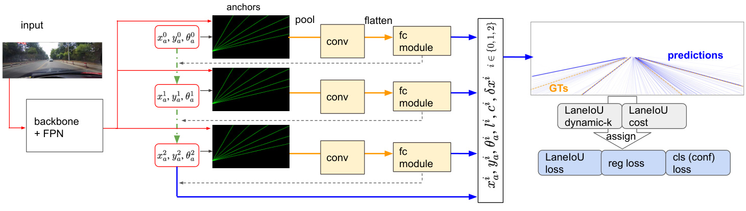
Figure 2: Network Schematic of CLRerNet.
图 2: CLRerNet 网络结构示意图。
Next, we calculate the metric IoU between predictions and GTs as the oracle confidence scores. For each prediction, the maximum IoU among the GTs is employed as the oracle score. In this case, the predicted lane coordinates are not changed. The $\mathrm{F}1_{50}$ jumps to 98.47 - the near-perfect score (second row). The result suggests that the correct lanes are already among the predictions, however the confidence scores need to be predicted accurately representing the metric IoU.
接下来,我们计算预测与真实标注(GTs)之间的交并比(IoU)指标作为基准置信度分数。对于每个预测,采用其与所有真实标注的最大IoU作为基准分数。此时预测车道坐标保持不变。$\mathrm{F}1_{50}$指标跃升至98.47——接近完美的分数(第二行)。结果表明正确车道已存在于预测结果中,但需要准确预测能反映IoU指标的置信度分数。
The other components are the anchor parameters - $x_{a}$ $y_{a}$ , $\theta_{a}$ and length $l$ that determine the lane coordinates. We alter the anchor parameters and lane length by those of GTs (third and fourth rows respectively). Although the row-wise refinement $\delta x$ is not changed, the oracle anchor parameters improve $\mathrm{F}1_{50}$ by 9 points. On the other hand, the oracle length does not affect the performance significantly. The results lead to the second suggestion that the anchor parameters $(x_{a},y_{a},\theta_{a})$ are important in terms of lane localization.
其他组件是确定车道坐标的锚点参数 - $x_{a}$、$y_{a}$、$\theta_{a}$ 以及长度 $l$。我们通过GT(分别为第三行和第四行)修改锚点参数和车道长度。尽管逐行细化 $\delta x$ 未改变,但理想锚点参数将 $\mathrm{F}1_{50}$ 提高了9个百分点。另一方面,理想长度对性能影响不大。这些结果得出第二个建议:锚点参数 $(x_{a}, y_{a}, \theta_{a})$ 在车道定位方面至关重要。
We focus on the first finding and aim to learn highquality confidence scores by improving the lane similarity function.
我们聚焦于第一个发现,旨在通过改进车道相似度函数来学习高质量置信度分数。
3.3. LaneIoU
3.3. LaneIoU
The existing methods [15] and [28] exploit horizontal distance and horizontal IoU as similarity functions respectively. However, these definitions do not match the metric IoU calculated with segmentation masks. For instance, when the lanes are tilted, the horizontal distance corresponding to the certain metric-IoU is larger than that of vertical lanes. To bridge the gap, we introduce a differentiable local-angle-aware IoU definition, namely LaneIoU. Fig. 3 shows an example of IoU calculation between two tilted curves. We compare LineIoU [28] and LaneIoU on the same lane instance pair. LineIoU applies a constant virtual width regardless of the lane angle and the virtual lane gets ’thin’ at the tilted part. In our LaneIoU, overlap and union are calculated considering the tilt of the local lane parts at each row. We define $\Omega_{p q}$ as the set of y slices where both lanes $p$ and $q$ exist, and $\Omega_{p}$ or $\Omega_{q}$ where only one lane exists. LaneIoU is calculated as:
现有方法[15]和[28]分别利用水平距离和水平IoU作为相似度函数。然而这些定义与通过分割掩码计算的度量IoU并不匹配。例如当车道倾斜时,特定度量IoU对应的水平距离会大于垂直车道的情况。为消除这一差异,我们提出了一种可微分的局部角度感知IoU定义——LaneIoU。图3展示了两条倾斜曲线间的IoU计算示例,我们在同一对车道实例上比较了LineIoU[28]与LaneIoU:LineIoU采用固定虚拟宽度而忽略车道角度,导致倾斜部分的虚拟车道变"细";而LaneIoU在计算重叠和并集时考虑了每行局部车道段的倾斜角度。定义$\Omega_{pq}$为两条车道$p$和$q$同时存在的y切片集合,$\Omega_{p}$或$\Omega_{q}$为单条车道存在的区域,则LaneIoU计算公式为:
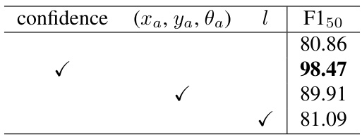
Table 1: Oracle experiment results.
表 1: Oracle实验结果。
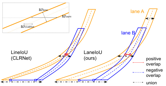
Figure 3: Example of LineIoU [28] and LaneIoU calcula- tions between laneA and laneB. $w_{l a n e}$ , $w_{C L R N e t}$ and $w_{o u r s}$ within the dashed rectangle stand for the lane width, the constant width of [28] and our angle-aware width.
图 3: 车道线A与车道线B之间的LineIoU [28]和LaneIoU计算示例。虚线框内的$w_{lane}$、$w_{CLRNet}$和$w_{ours}$分别表示车道宽度、[28]的恒定宽度和我们的角度感知宽度。
$$
L a n e I o U=\frac{\sum_{i=0}^{H}{I_{i}}}{\sum_{i=0}^{H}{U_{i}}}
$$
$$
L a n e I o U=\frac{\sum_{i=0}^{H}{I_{i}}}{\sum_{i=0}^{H}{U_{i}}}
$$
where $I_{i}$ and $U_{i}$ are defined as:
其中 $I_{i}$ 和 $U_{i}$ 定义为:
$$
\begin{array}{r}{I_{i}=\operatorname*{min}(x_{i}^{p}+w_{i}^{p},x_{i}^{q}+w_{i}^{q})-\operatorname*{max}(x_{i}^{p}-w_{i}^{p},x_{i}^{q}-w_{i}^{q})}\ {U_{i}=\operatorname*{max}(x_{i}^{p}+w_{i}^{p},x_{i}^{q}+w_{i}^{q})-\operatorname*{min}(x_{i}^{p}-w_{i}^{p},x_{i}^{q}-w_{i}^{q})}\end{array}
$$
$$
\begin{array}{r}{I_{i}=\operatorname*{min}(x_{i}^{p}+w_{i}^{p},x_{i}^{q}+w_{i}^{q})-\operatorname*{max}(x_{i}^{p}-w_{i}^{p},x_{i}^{q}-w_{i}^{q})}\ {U_{i}=\operatorname*{max}(x_{i}^{p}+w_{i}^{p},x_{i}^{q}+w_{i}^{q})-\operatorname*{min}(x_{i}^{p}-w_{i}^{p},x_{i}^{q}-w_{i}^{q})}\end{array}
$$
when $i\in\Omega_{p q}$ . The intersection of the lanes is positive when the lanes are overlapped and negative otherwise. If $i\notin\Omega_{p q}$ , $I_{i}$ and $U_{i}$ are calculated as follows:
当 $i\in\Omega_{p q}$ 时。当车道重叠时,车道交集为正,否则为负。如果 $i\notin\Omega_{p q}$ ,则 $I_{i}$ 和 $U_{i}$ 的计算方式如下:
$$
\begin{array}{l}{I_{i}=0,U_{i}=2w_{i}^{k}\mathrm{if}k\in{p,q},i\in\Omega_{k}}\ {\quad}\ {I_{i}=0,U_{i}=0\mathrm{if}i\notin(\Omega_{p q}\cup\Omega_{p}\cup\Omega_{q})}\end{array}
$$
$$
\begin{array}{l}{I_{i}=0,U_{i}=2w_{i}^{k}\mathrm{if}k\in{p,q},i\in\Omega_{k}}\ {\quad}\ {I_{i}=0,U_{i}=0\mathrm{if}i\notin(\Omega_{p q}\cup\Omega_{p}\cup\Omega_{q})}\end{array}
$$
The virtual lane widths $w_{i}^{p}$ and $w_{i}^{q}$ are calculated taking the local angles into consideration:
虚拟车道宽度 $w_{i}^{p}$ 和 $w_{i}^{q}$ 的计算考虑了局部角度:
$$
w_{i}^{k}=\frac{w_{l a n e}}{2}\frac{\sqrt{(\Delta x_{i}^{k})^{2}+(\Delta y_{i}^{k})^{2}}}{\Delta y_{i}^{k}}
$$
$$
w_{i}^{k}=\frac{w_{l a n e}}{2}\frac{\sqrt{(\Delta x_{i}^{k})^{2}+(\Delta y_{i}^{k})^{2}}}{\Delta y_{i}^{k}}
$$
where $k\in{p,q}$ and $\Delta x_{i}$ and $\Delta y_{i}$ stand for the local changes of the lane point coordinates. Equation 7 compensates the tilt variation of lanes and represents a general row-wise lane IoU calculation. When the lanes are vertical, $w_{i}$ equals to $w_{l a n e}/2$ and gets larger as the lanes tilt. $w_{l a n e}$ is the parameter which controls the strictness of the IoU calculation. The CULane metric employs 30 pixels for the resolution of (590, 1640).
其中 $k\in{p,q}$ ,$\Delta x_{i}$ 和 $\Delta y_{i}$ 表示车道点坐标的局部变化。公式7补偿了车道的倾斜变化,代表了一种通用的逐行车道IoU计算方法。当车道垂直时,$w_{i}$ 等于 $w_{l a n e}/2$ ,并随着车道倾斜而增大。$w_{l a n e}$ 是控制IoU计算严格程度的参数。CULane指标在(590, 1640)分辨率下采用30像素。
In Fig. 4, LineIoU [28] and our LaneIoU are compared by calculating correlation with the CULane metric. We replace each prediction’s confidence score with the LineIoU or LaneIoU value and also calculate the metric IoU. The GT with the largest IoU is chosen for each prediction. Clearly our LaneIoU shows better correlation with the metric IoU mainly as the result of eliminating the influence of lane angles.
在图4中,通过计算与CULane指标的关联性,对比了LineIoU [28]和我们的LaneIoU。我们将每条预测的置信度分数替换为LineIoU或LaneIoU值,同时计算指标IoU。对于每条预测,选择具有最大IoU的真值(GT)。显然,我们的LaneIoU与指标IoU表现出更好的相关性,这主要得益于消除了车道角度的影响。
3.4. Sample assignment
3.4. 样本分配
The confidence scores are learned to be high if the anchor is assigned as positive during training. We adopt LaneIoU for sample assignment to bring the detector’s confidence scores close to the segmentation-based IoU. [28] employs the SimOTA assigner [5] to dynamically assign $k_{i}$ anchors for each GT lane $t_{i}$ . The number of anchors $k_{i}$ is determined by calculating the sum of all the anchors’ positive IoUs. We employ LaneIoU as:
置信度得分在训练中被学习为高值,当锚点被分配为正样本时。我们采用LaneIoU进行样本分配,以使检测器的置信度得分更接近基于分割的IoU。[28] 使用SimOTA分配器 [5] 动态地为每个真实车道线 (GT lane) $t_{i}$ 分配 $k_{i}$ 个锚点。锚点数量 $k_{i}$ 通过计算所有锚点的正样本IoU之和确定。我们采用LaneIoU如下:
$$
k_{i}=\sum_{j=1}^{m}L a n e I o U(p_{j},t_{i})
$$
$$
k_{i}=\sum_{j=1}^{m}L a n e I o U(p_{j},t_{i})
$$
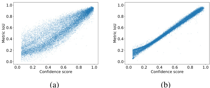
Figure 4: Correlation between CULane metric IoU and (a) LineIoU [28] and (b) LaneIoU (ours).
图 4: CULane指标IoU与(a) LineIoU [28] 和(b) LaneIoU(本文提出的)之间的相关性。
where $m$ is the number of anchors and $i~=~0,1,...,n$ is the index of $n$ GT lanes. $p_{j}$ is a predicted lane and $j=0,1,...,m$ is the index of $m$ predictions. $k_{i}$ is clipped to be from 1 to $k_{m a x}$ . The cost matrix determines the priority of the assignment for each GT. In object detection, [5] adopts the sum of bounding box IoU and classification costs. In lane detection, CLRNet [28] utilizes the classification cost and the lane similarity cost which consists of horizontal distance, angle difference and start-point distance. However, the cost that directly represents the evaluation metric is more straightforward for prioritizing predictions. We define the cost matrix as:
其中 $m$ 是锚点数量,$i~=~0,1,...,n$ 是 $n$ 条真实车道线的索引。$p_{j}$ 是预测车道线,$j=0,1,...,m$ 是 $m$ 条预测结果的索引。$k_{i}$ 被截断至1到 $k_{m a x}$ 之间。该成本矩阵决定了每条真实车道线的匹配优先级。在目标检测中,[5] 采用边界框IoU与分类成本的求和。在车道线检测中,CLRNet [28] 使用了分类成本及由水平距离、角度差和起点距离构成的车道相似性成本。但直接反映评估指标的成本能更直观地为预测结果排序。我们将成本矩阵定义为:
$$
c o s t_{j i}=-L a n e I o U_{n o r m}(p_{j},t_{i})+\lambda f_{c l a s s}(p_{j},t_{i})
$$
$$
c o s t_{j i}=-L a n e I o U_{n o r m}(p_{j},t_{i})+\lambda f_{c l a s s}(p_{j},t_{i})
$$
where $\lambda$ is the parameter to balance the two costs and $f_{c l a s s}$ is the cost function for classification, such as a focal loss [14]. LaneIoU is normalized from its minimum to maximum. The formulation (eq. 8 and 9) realizes dynamic sample assignment of the proper number of anchors which are prioritized according to the evaluation metric. In summary, compared with CLRNet, our CLRerNet introduces LaneIoU as the dynamic $\mathbf{\nabla\cdotk}$ assignment function, assignment cost function and loss function to learn the high-quality confidence scores that better correlate with the metric IoU.
其中 $\lambda$ 是平衡两项损失的参数,$f_{class}$ 是分类损失函数(如焦点损失 [14])。LaneIoU 会进行最小最大值归一化处理。公式(式 8 和式 9)实现了动态样本分配机制,能根据评估指标优先选择适当数量的锚点。总体而言,相较于 CLRNet,我们的 CLRerNet 引入了 LaneIoU 作为动态 $\mathbf{\nabla\cdotk}$ 分配函数、分配损失函数以及训练损失函数,从而学习到与度量指标 IoU 相关性更高的高质量置信分数。
4. Experiments
4. 实验
4.1. Datasets
4.1. 数据集
The CULane dataset1[18] is the de-facto standard lane detection benchmark dataset which contains 88,880 train frames, 9,675 validation frames, and 34,680 test frames with lane point annotations. The test split has frame-based scene annotations such as Normal, Crowded and Curve (see Table 2). The Curve Lanes 2 [7] dataset contains the challenging curve scenes and consists of $100\mathrm{k}$ train, $20\mathrm{k\Omega}$ val and 30k test frames. We follow [15] and use the val split for evaluation.
CULane数据集[18]是车道检测领域事实上的标准基准数据集,包含88,880帧训练图像、9,675帧验证图像和34,680帧带有车道点标注的测试图像。测试集细分了基于帧的场景标注,如正常(Normal)、拥堵(Crowded)和弯道(Curve)场景(见表2)。Curve Lanes 2[7]数据集包含具有挑战性的弯道场景,由$100\mathrm{k}$训练帧、$20\mathrm{k\Omega}$验证帧和30k测试帧组成。我们遵循[15]的做法,使用验证集进行评估。
Removing the redundant train data. The CULane dataset includes a non-negligible amount of redundant frames where the ego-vehicle is stationary and the lane annotations do not change. We have found that over fitting to the redundant frames can be avoided by simply removing the frames whose average pixel value difference from the previous frame is below a threshold. The optimal threshold $(=15)$ is chosen empirically via validation as described in the supplementary material. The remaining 55,698 $(62.7%)$ frames are utilized for training. The F1 score of CLRNet-DLA34 is improved from $80.30{\pm}0.05$ to $80.86{\pm}0.06$ $N=5$ each) with the same 15-epoch training.
移除冗余训练数据。CULane数据集中包含大量冗余帧,这些帧中自车静止且车道标注未发生变化。我们发现,只需移除与前一帧平均像素差值低于阈值的帧(经验证选定最优阈值为 $(=15)$,详见补充材料),即可避免对冗余帧的过拟合。剩余55,698帧(占比 $(62.7%)$ )用于训练后,CLRNet-DLA34的F1分数从 $80.30{\pm}0.05$ 提升至 $80.86{\pm}0.06$ ( $N=5$ 次实验均值),训练周期保持15轮不变。
4.2. Training and evaluation
4.2. 训练与评估
The models are implemented on PyTorch and MMDetection [3], and are trained for 15 epochs with AdamW [17] optimizer. The initial learning rate is 0.0006 and cosine decay is applied. For CULane dataset, we crop the input image below $y=270$ and resize it to (800, 320) pixels. Horizontal flip, random brightness and contrast, random HSV modulation, motion and median blur and random affine modulations are adopted as data augmentation, following [28]. At the test time only the crop and resize are adopted and no test-time augmentations are applied. In CLRerNet, LaneIoU is introduced as a loss function, dynamic $\mathbf{\nabla\cdotk}$ calculation and assignment loss function. $w_{l a n e}$ is set to 15/800 for loss and dynamic-k, and 60/800 for cost to balance with the classification cost. The loss weights in eq. 1 are the same as [28] except for $\lambda_{3}$ which is set to 4. We additionally benchmark a CLRerNet-DLA34 model trained for 60 epochs applying exponential moving average (EMA). The learning rate decay is not applied and the momentum of EMA is set to 0.0001.
模型基于PyTorch和MMDetection [3]实现,采用AdamW [17]优化器训练15个周期。初始学习率为0.0006并应用余弦衰减。对于CULane数据集,我们将输入图像在$y=270$以下区域裁剪并调整至(800, 320)像素。数据增强策略包括水平翻转、随机亮度对比度调整、随机HSV调制、运动与中值模糊以及随机仿射变换[28]。测试阶段仅进行裁剪和尺寸调整,不采用测试时增强。CLRerNet中引入LaneIoU作为损失函数,包含动态$\mathbf{\nabla\cdotk}$计算和分配损失函数。$w_{l a n e}$在损失和动态k计算中设为15/800,在成本计算中设为60/800以平衡分类成本。公式1中的损失权重与[28]相同,但$\lambda_{3}$设为4。我们还测试了采用指数移动平均(EMA)训练60个周期的CLRerNet-DLA34模型,其中未应用学习率衰减且EMA动量设为0.0001。
To validate the generality of our method, we add the LaneIoU-based sample assignment to LaneATT[24]. Originally, LaneATT assigns non-learnable static anchors to GTs by horizontal distance threshold ing. We prioritize the anchors by calculating LaneIoU between predicted lanes and GTs to assign the positive-confidence targets. More details are described in the supplementary material.
为验证方法的通用性,我们将基于LaneIoU的样本分配策略引入LaneATT[24]。原版LaneATT通过水平距离阈值将静态锚点(non-learnable static anchors)分配给真实车道线(GTs)。我们通过计算预测车道线与真实车道线之间的LaneIoU来优先分配正置信度目标(positive-confidence targets)。补充材料提供了更多细节说明。
For CurveLanes [7], we follow the training setting of [15] where the input resolution is (800, 320). To exploit the auxiliary segmentation loss, we draw the segmentation mask along all the lane labels with width of 30 pixels. Different from [18], we set all the lane masks as class one (foreground). Since the test annotations are not available, we evaluate our method on the validation split. We employ the evaluation resolution of (224, 224) and line width of 5 following [15]. $w_{l a n e}$ is set to 5/224 for loss and dynamic $\boldsymbol{\cdot}\mathbf{k}$ calculation and $20/224$ for cost. $\lambda$ for assignment cost calculation (eq. 9) is set to 2.5.
对于CurveLanes [7],我们遵循[15]的训练设置,输入分辨率为(800, 320)。为了利用辅助分割损失,我们沿所有车道标签绘制了宽度为30像素的分割掩码。与[18]不同,我们将所有车道掩码设置为类别一(前景)。由于测试标注不可用,我们在验证集上评估我们的方法。采用[15]的评估分辨率(224, 224)和5像素线宽。损失计算和动态$\boldsymbol{\cdot}\mathbf{k}$计算中$w_{lane}$设为5/224,代价计算中设为$20/224$。分配代价计算(公式9)中的$\lambda$设为2.5。
Evaluation metric. We employ F1 score [18] as an evaluation metric. An IoU matrix between predicted lanes and ground-truths is calculated by comparing the segmentation masks drawn with a width of 30 pixels (Fig. 1 bottom). Based on the IoU matrix, one-to-one matching is calculated using linear sum assignment and the prediction-GT pairs with IoU over $t_{I o U}$ are considered as true positives $(T P)$ . Unmatched predictions and GTs are counted as false positives $(F P)$ and false negatives $(F N)$ respectively. We employ two $t_{I o U}$ values for IoU calculation: 0.5 and 0.75. The F1 score is calculated as:
评估指标。我们采用F1分数[18]作为评估指标。通过比较宽度为30像素的分割掩码(图1底部),计算预测车道线与真实标注之间的IoU矩阵。基于该矩阵,使用线性求和分配计算一对一匹配,IoU超过$t_{I o U}$的预测-真实值对被视作真阳性$(T P)$。未匹配的预测和真实标注分别计为假阳性$(F P)$和假阴性$(F N)$。我们采用两个$t_{I o U}$值进行IoU计算:0.5和0.75。F1分数计算公式为:

Figure 5: Qualitative results comparing LaneATT, CLRNet and our CLRerNe $\cdot^{+\star}$ . Predictions and GTs are shown in blue and orange respectively. Predictions with insufficient confidence score are shown as blue circles.
图 5: LaneATT、CLRNet 与我们的 CLRerNe$\cdot^{+\star}$定性对比结果。预测结果和真实标注 (GT) 分别用蓝色和橙色表示,置信度不足的预测结果以蓝色圆圈标注。
$$
F_{1}=\frac{2\times P r e c i s i o n\times R e c a l l}{P r e c i s i o n+R e c a l l}
$$
$$
F_{1}=\frac{2\times P r e c i s i o n\times R e c a l l}{P r e c i s i o n+R e c a l l}
$$
Cross validation and test. The F1 metric is sensitive to the threshold of detection confidence score. We perform 5-fold cross validation on the train split, by randomly dividing the train videos into five groups. The F1 score of each threshold is averaged across the 5-fold results, and the optimal threshold is determined by taking the argmax of it.
交叉验证与测试。F1指标对检测置信度分数的阈值较为敏感。我们在训练集上进行了5折交叉验证,随机将训练视频划分为五组。每个阈值对应的F1分数取五折结果的平均值,最终通过argmax确定最优阈值。
Moreover, we find that the F1 score deviation of the models trained with different random seeds is not negligible. For instance, the F1 score of the CLRNet-DLA34 ranges from the minimum of 80.20 to the maximum of 80.34 ( $N=5$ ). For a more reliable and fairer benchmark on the test split, we train five models with different random seeds for each condition and calculate the mean and standard deviation of the metrics, on which the confidence thresholds obtained by five-fold cross validation is applied. To the best of our knowledge, we are the first to conduct the above benchmark protocol in lane detection. As for the CurveLanes dataset where the test annotations are not available, we report the maximum F1 score on the validation split with respect to the confidence thresholds.
此外,我们发现不同随机种子训练的模型在F1分数上的偏差不可忽视。例如,CLRNet-DLA34的F1分数最低为80.20,最高为80.34($N=5$)。为了在测试集上获得更可靠、更公平的基准结果,我们为每种条件训练了五个不同随机种子的模型,并计算指标的平均值和标准差,在此基础上应用通过五折交叉验证得到的置信度阈值。据我们所知,我们是首个在车道检测任务中采用上述基准协议的团队。对于测试标注不可用的CurveLanes数据集,我们报告了验证集上相对于置信度阈值的最大F1分数。
4.3. CULane benchmark results
4.3. CULane 基准测试结果
The benchmark results on the CULane test set are shown in Table 2. The rows below the double horizontal line are our experiment results. For each condition (row), we show the averaged metric values of five models trained with different seeds. The confidence threshold obtained from 5- fold cross-validation is employed. The $\mathrm{F}1_{50}$ scores are shown in the test scene columns except for the cross metric where the number of false positives is shown. All the FPS results on Table 2 are measured with a GeForce RTX 3090 GPU. CLRNet† and LaneATT† are the baseline model trained with our implementation. Our method CLRerNet† employs LaneIoU for dynamic $\mathbf{\nabla\cdot}\mathbf{k}$ calculation, assignment cost and loss functions. CLRerNet $\dag\star$ is the boosted version of CLRerNet† which is trained for 60 epochs with EMA.
CULane测试集的基准结果如表2所示。双横线下方各行是我们的实验结果。每种条件(行)展示了用不同随机种子训练的五个模型的平均指标值。采用通过五折交叉验证获得的置信度阈值。除交叉指标显示误报数量外,测试场景列均展示$\mathrm{F}1_{50}$分数。表2中所有FPS结果均在GeForce RTX 3090 GPU上测得。CLRNet†和LaneATT†是我们实现训练的基线模型。我们的CLRerNet†方法采用LaneIoU进行动态$\mathbf{\nabla\cdot}\mathbf{k}$计算、分配代价及损失函数。CLRerNet$\dag\star$是CLRerNet†的增强版本,通过EMA训练60个周期。
Table 2: Evaluation results on the CULane test set. Our experiments are below the double horizontal line.
| 方法 | 骨干网络 | F150 | F175 | Normal | Crowd | Dazzle | Shadow | Noline | Arrow | Curve | Cross | Night | GFLOPs | FPS |
|---|---|---|---|---|---|---|---|---|---|---|---|---|---|---|
| SCNN | VGG16 | 71.60 | 39.84 | 90.60 | 69.70 | 58.50 | 66.90 | 43.40 | 84.10 | 64.40 | 1990 | 66.10 | 218.6 | 50 |
| LaneATT | Res18 | 75.13 | 51.29 | 91.17 | 72.71 | 65.82 | 68.03 | 49.13 | 87.82 | 63.75 | 1020 | 68.58 | 9.3 | 211 |
| LaneATT | Res34 | 76.68 | 54.34 | 92.14 | 75.03 | 66.47 | 78.15 | 49.39 | 88.38 | 67.72 | 1330 | 70.72 | 18.0 | 170 |
| CondLane[15] | Res18 | 78.14 | 57.42 | 92.87 | 75.79 | 70.72 | 80.01 | 52.39 | 89.37 | 72.40 | 1364 | 73.23 | 10.2 | 348 |
| CondLane[15] | Res34 | 78.74 | 59.39 | 93.38 | 77.14 | 71.17 | 79.93 | 51.85 | 89.89 | 73.88 | 1387 | 73.92 | 19.6 | 237 |
| CondLane[15] | Res101 | 79.48 | 61.23 | 93.47 | 77.44 | 70.93 | 80.91 | 54.13 | 90.16 | 75.21 | 1201 | 74.80 | 44.8 | 97 |
| CLRNet[28] | Res34 | 79.73 | 62.11 | 93.49 | 78.06 | 74.57 | 79.92 | 54.01 | 90.59 | 72.77 | 1216 | 75.02 | 21.5 | 204 |
| CLRNet[28] | Res101 | 80.13 | 62.96 | 93.85 | 78.78 | 72.49 | 82.33 | 54.50 | 89.79 | 75.57 | 1262 | 75.51 | 42.9 | 94 |
| CLRNet[28] | DLA34 | 80.47 | 62.78 | 93.73 | 79.59 | 75.30 | 82.51 | 54.58 | 90.62 | 74.13 | 1155 | 75.37 | 18.4 | 185 |
| LaneATTt | Res34 | 77.51±0.10 | 56.78 | 92.48 | 75.47 | 68.09 | 73.21 | 50.96 | 88.72 | 68.18 | 1054 | 72.58 | 18.0 | 170 |
| CLRNett | Res34 | 80.54±0.12 | 63.65 | 93.85 | 79.22 | 73.32 | 82.50 | 55.26 | 90.84 | 74.06 | 1106 | 75.92 | 21.5 | 204 |
| CLRNett | Res101 | 80.67±0.06 | 64.35 | 93.95 | 79.60 | 72.91 | 81.58 | 55.76 | 90.42 | 74.06 | 1166 | 76.01 | 42.9 | 94 |
| CLRNett | DLA34 | 80.86±0.06 | 64.05 | 94.03 | 79.78 | 75.23 | 81.94 | 56.02 | 90.67 | 74.57 | 1184 | 76.40 | 18.4 | 185 |
| LaneATT+↑ | Res34 | 78.19±0.06 | 56.96 | 92.60 | 76.42 | 69.12 | 77.59 | 52.01 | 88.75 | 64.49 | 974 | 72.78 | 18.0 | 153 |
| CLRerNett | Res34 | 80.76±0.13 | 63.77 | 93.93 | 79.51 | 73.88 | 83.16 | 55.55 | 90.87 | 74.45 | 1088 | 76.02 | 21.5 | 204 |
| CLRerNett | Res101 | 80.91±0.10 | 64.30 | 93.91 | 80.03 | 72.98 | 82.92 | 55.73 | 90.53 | 73.83 | 1113 | 76.13 | 42.9 | 94 |
| CLRerNett | DLA34 | 81.12±0.04 | 64.07 | 94.02 | 80.20 | 74.41 | 83.71 | 56.27 | 90.39 | 74.67 | 1161 | 76.53 | 18.4 | 185 |
| CLRerNet* | DLA34 | 81.43±0.14 | 65.06 | 94.36 | 80.62 | 75.23 | 84.35 | 57.31 | 91.17 | 79.11 | 1540 | 76.92 | 18.4 | 185 |
表 2: CULane测试集上的评估结果。我们的实验结果在双横线下方。
With introducing LaneIoU, CLRerNet† with DLA34 outperforms CLRNet by $0.26%$ in $\mathrm{F}1_{50}$ . Moreover, the boosted model CLRerNet $\dag\star$ reaches $\mathrm{F1_{50}=81.43%}$ in average, enjoying the state-of-the-art performance surpassing the previous methods $(\mathrm{F1_{50}~=~80.47%}$ , single ex- periment of CLRNet+DLA34) by a large margin. The performance improvement by LaneIoU is also observed on the models with other backbones - $80.54%$ to $80.76%$ $(+0.22%)$ with ResNet34 and $80.67%$ to $80.91%$ $(+0.24%)$ with ResNet101. LaneATT $^{+\dagger}$ is improved by the LaneIoUbased assignment by $0.68%$ , validating the generality of our method. CLRerNet does not increase test-time computational complexity and shows the same GFLOPs and FPS as CLRNet.
引入LaneIoU后,采用DLA34的CLRerNet†在$\mathrm{F}1_{50}$指标上以$0.26%$的优势超越CLRNet。此外,增强版模型CLRerNet$\dag\star$平均达到$\mathrm{F1_{50}=81.43%}$,以显著优势超越先前方法$(\mathrm{F1_{50}~=~80.47%}$,即CLRNet+DLA34单次实验) 取得最先进性能。LaneIoU带来的性能提升在其他骨干网络模型中也得到验证:ResNet34从$80.54%$提升至$80.76%$$(+0.22%)$,ResNet101从$80.67%$提升至$80.91%$$(+0.24%)$。基于LaneIoU的分配策略使LaneATT$^{+\dagger}$提升$0.68%$,证实了方法的通用性。CLRerNet未增加测试时计算复杂度,其GFLOPs和FPS与CLRNet保持相同。
Qualitative results on the CULane test set are shown in Fig. 5. Our CLRerNe $\cdot^{\dagger\star}$ is capable of detecting the lanes in the challenging scenes. The right-most tilted lane of the first image (top) and the left-most lane of the second image (bottom) are detected only by CLRerNet with high confidence scores. The examples qualitatively suggest that CLRerNet is able to give more correct scores to predictions, which is analyzed in Subsection 4.5.
在CULane测试集上的定性结果如图5所示。我们的CLRerNe $\cdot^{\dagger\star}$ 能够在具有挑战性的场景中检测车道线。第一张图(上)最右侧倾斜车道和第二张图(下)最左侧车道仅被CLRerNet以高置信度分数检测到。这些示例定性地表明CLRerNet能够为预测给出更准确的分数,具体分析见第4.5小节。
| 方法 | F1 | 精确率 (Precision) | 召回率 (Recall) | GFLOPs |
|---|---|---|---|---|
| CondLane-S[15] | 85.09 | 87.75 | 82.58 | 10.3 |
| CondLane-M[15] | 85.92 | 88.29 | 83.68 | 19.7 |
| CondLane-L[15] | 86.10 | 88.98 | 83.41 | 44.9 |
| CLRNet-DLA34[28] | 86.10±0.08 | 91.40 | 81.39 | 18.4 |
| CLRerNet-DLA34 | 86.47±0.07 | 91.66 | 81.83 | 18.4 |
Table 3: Comparison between methods on the CurveLanes val set. Our experiments are below the double horizontal line.
表 3: CurveLanes验证集上的方法对比。我们的实验结果在双横线下方。
4.4. CurveLanes validation results
4.4 CurveLanes验证结果
The validation results on CurveLanes are shown in Table 3. The default CLRNet [28] with the DLA34 backbone shows the same F1 score as CondLane-L[15] with lower computation cost. Note that our results are the average of five training trials. The confidence threshold is set to the empirically optimal value 0.44. CLRerNet significantly outperforms the baseline by $0.37%$ , achieving the new stateof-the-art $86.47%$ .
CurveLanes上的验证结果如表3所示。采用DLA34骨干网络的默认CLRNet [28]与CondLane-L[15]的F1分数相同,但计算成本更低。请注意,我们的结果是五次训练试验的平均值。置信度阈值设置为经验最优值0.44。CLRerNet显著超越基线 $0.37%$ ,达到新的最先进水平 $86.47%$ 。
4.5. Ablation study and analysis
4.5. 消融研究与分析
We corroborate the effectiveness of our method by ablating LaneIoU from dynamic $\mathbf{\nabla\cdotk}$ calculation, assignment cost and loss function. CLRerNet with DLA34 backbone is trained in each condition with the redundant train data omitted. We follow the benchmark protocol described in subsection 4.2, thus ten models (5 seeds $+5$ folds) are trained and validated for each condition. The results in Table 4 show that the performance degrades by replacing LaneIoU with [28] for dynamic-k determination, cost function and loss function respectively. Determining the number of assignments each GT lane by LaneIoU mitigates the inhomogeneity caused by lane tilt variation. The LaneIoU-based assignment cost (eq. 9) prioritizes the predicted lanes which have higher metric IoU with the GTs, leading to more accurate confidence learning as motivated in subsection 3.2. Replacing LineIoU loss with LaneIoU loss also mitigates the tilt dependency of the regression penalty.
我们通过从动态$\mathbf{\nabla\cdotk}$计算、分配代价和损失函数中消融LaneIoU来验证方法的有效性。采用DLA34骨干网的CLRerNet在每种条件下训练时均省略冗余训练数据。遵循4.2小节描述的基准协议,每种条件训练并验证十个模型(5次随机种子$+5$折交叉验证)。表4结果显示:分别在动态k确定、代价函数和损失函数中用[28]替代LaneIoU会导致性能下降。基于LaneIoU确定每条GT车道的分配数量,可缓解车道倾斜变化导致的非均匀性问题。基于LaneIoU的分配代价(公式9)会优先选择与GT具有更高度量IoU的预测车道,如3.2小节所述,这能实现更准确的置信度学习。用LaneIoU损失替代LineIoU损失还能减弱回归惩罚对倾斜角度的依赖性。
| dynamic-k | cost | loss | F150 | F175 |
|---|---|---|---|---|
| [28] | [28] | [28] | 80.86±0.06 | 64.05±0.17 |
| LaneIoU | [28] | [28] | 80.98±0.07 | 64.17±0.17 |
| LaneIoU | LaneloU | [28] | 81.07±0.03 | 64.22±0.26 |
| LaneloU | LaneloU | LaneloU | 81.12±0.05 | 64.28±0.15 |

Table 4: Ablation study by replacing LaneIoU (ours) with [28].
表 4: 用[28]替换LaneIoU(ours)的消融研究
Fig. 6 shows the comparison between CLRerNet and CLRNet in terms of anchor assignment numbers per GT in different angle ranges. The assignment numbers are accumulated during the training and averaged. The angles are calculated using GT lanes in (800, 320) resolution and $90^{\circ}$ corresponds to the vertical lane. By leveraging LaneIoU, the assignment number becomes more homogeneous with respect to the lane angles, especially in the angle ranges of $20^{\circ}$ to $60^{\circ}$ and $120^{\circ}$ to $160^{\circ}$ where the GTs typically exist.
图 6 展示了 CLRerNet 和 CLRNet 在不同角度范围内每个 GT (ground truth) 的锚点分配数量对比。分配数量在训练过程中累计并取平均值。角度使用 (800, 320) 分辨率下的 GT 车道线计算,其中 $90^{\circ}$ 对应垂直车道。通过采用 LaneIoU,分配数量在不同车道角度下分布更均匀,尤其在 $20^{\circ}$ 至 $60^{\circ}$ 和 $120^{\circ}$ 至 $160^{\circ}$ 的典型 GT 存在角度范围内表现显著。
The assigned anchor’s confidence target is set to positive prioritized by LaneIoU. Therefore, the confidence is trained more homogeneously across different lane angles. As can be seen in Fig. 7, the $l1$ error between the predicted confidence scores and the metric IoU values is improved in CLRerNet in the non-vertical angle ranges, corroborating the effectiveness of LaneIoU.
分配锚点的置信度目标设置为由LaneIoU优先确定的正值。因此,在不同车道角度下,置信度的训练更加均匀。如图7所示,在非垂直角度范围内,CLRerNet中预测置信度分数与度量IoU值之间的$l1$误差有所改善,这验证了LaneIoU的有效性。
Discussion. Although CLRerNet shows significant improvement in performance, there still is a gap between the best CLRerNet model’s performance $(81.43%)$ and the oracle-confidence case $(98.47%)$ . The dataset-oriented issues including label fluctuation and data imbalance are considered to be the part of the gap. For instance, there are the cases in the CULane test set where detection is extremely difficult (Fig. 8). As can be found in Table 2, the Noline test category is the most challenging as there are no visual markings on the road. Such cases are prone to label fluctuation and inconsistency. Likewise, data imbalance such as stationary scenes greatly affects the model training. As is mentioned in Subsection 4.1, we find that mitigating the data imbalance significantly improves the performance.
讨论。尽管CLRerNet在性能上展现出显著提升,但其最佳模型表现 $(81.43%)$ 与理论置信上限 $(98.47%)$ 之间仍存在差距。标签波动和数据不平衡等数据集相关问题被认为是造成部分差距的原因。例如,CULane测试集中存在检测难度极高的案例(图8)。如表2所示,无标线(Noline)测试类别最具挑战性,因为道路上没有视觉标记。这类情况容易引发标签波动和不一致。同样,静态场景等数据不平衡问题会极大影响模型训练。如第4.1节所述,我们发现缓解数据不平衡能显著提升性能。

Figure 7: The average $l1$ error between confidence score and metric IoU in different angle ranges.
图 7: 不同角度范围内置信度分数与指标 IoU 之间的平均 $l1$ 误差。

Figure 6: The average number of assignments in different angle ranges. Figure 8: Extremely difficult cases in the CULane dataset. GTs are overlaid as orange circles.
图 6: 不同角度范围内的平均分配数量。图 8: CULane 数据集中极端困难的案例。GT (Ground Truth) 以橙色圆圈叠加显示。
5. Conclusion
5. 结论
We disentangle the lane prediction components by the oracle experiment and demonstrate the importance of highquality confidence scores for more accurate lane detection. To make confidence scores represent the metric IoU, the novel LaneIoU is proposed and integrated into the rowbased lane detection baselines. A novel detector coined CLRerNet is developed by introducing LaneIoU as the sample assignment and loss functions. The statistical and fair benchmark protocol is employed utilizing five-seed models and five-fold cross validation. CLRerNet achieves the state-of-the-art performance on the challenging CULane and CurveLanes datasets significantly surpassing the baseline. We believe our oracle experiments, LaneIoU-based training and benchmark protocol bring a clearer view of lane detection to the community.
我们通过理想实验解耦了车道线预测组件,并证明了高质量置信度分数对提升车道检测精度的重要性。为使置信度分数能准确反映交并比(IoU)指标,本文提出新型LaneIoU并将其集成至基于行的车道检测基线模型。通过将LaneIoU作为样本分配和损失函数,我们开发了新型检测器CLRerNet。采用五种子模型和五折交叉验证的统计公平基准协议,CLRerNet在CULane和CurveLanes挑战性数据集上显著超越基线模型,达到最先进性能。我们相信这些理想实验、基于LaneIoU的训练方案和基准协议将为学界带来更清晰的车道检测研究视角。