You Only Need One Color Space: An Efficient Network for Low-light Image Enhancement
你只需要一种色彩空间:一种用于低光图像增强的高效网络
Abstract—Low-Light Image Enhancement (LLIE) task tends to restore the details and visual information from corrupted lowlight images. Most existing methods learn the mapping function between low/normal-light images by deep neural networks on sRGB and HSV color space. However, these methods involve sensitivity and instability in the enhancement process, which often generate obvious color and brightness artifacts. To alleviate this problem, we propose a novel trainable color space, named Horizontal/Vertical-Intensity (HVI), which not only decouples brightness and color from RGB channels to mitigate the instability during enhancement, but also adapts to low-light images in different illumination ranges due to the trainable parameters. Furthermore, we design a novel Color and Intensity Decoupling Network (CIDNet) with two branches dedicated to processing the decoupled image brightness and color in the HVI space. In addition, we introduce the Lighten Cross-Attention (LCA) module to facilitate interaction between image structure and content information in both branches, while also suppressing noise in low-light images. We conduct 22 quantitative and qualitative experiments to show that the proposed CIDNet outperforms the state-of-the-art methods on 11 datasets. The code is available at https://github.com/Fediory/HVI-CIDNet.
摘要—低光照图像增强(LLIE)任务旨在从受损的低光照图像中恢复细节和视觉信息。现有方法大多通过在sRGB和HSV色彩空间上训练深度神经网络来学习低光/正常光图像间的映射函数。然而这些方法在增强过程中存在敏感性和不稳定性,常会产生明显的色彩与亮度伪影。为解决该问题,我们提出了一种新型可训练色彩空间HVI (Horizontal/Vertical-Intensity),该空间不仅通过从RGB通道解耦亮度与色彩来缓解增强过程中的不稳定性,还能通过可训练参数适应不同光照范围的低光图像。此外,我们设计了色彩与亮度解耦网络(CIDNet),采用双分支架构在HVI空间中分别处理解耦后的图像亮度和色彩信息。创新性地引入光照交叉注意力(LCA)模块促进双分支间图像结构与内容信息的交互,同时有效抑制低光图像噪声。通过22项定量与定性实验表明,所提出的CIDNet在11个数据集上均优于当前最先进方法。代码已开源:https://github.com/Fediory/HVI-CIDNet。
Index Terms—Low-Light Image Enhancement, HVI Color Space, Transformer, Supervised Learning.
索引术语—低光照图像增强 (Low-Light Image Enhancement)、HVI色彩空间 (HVI Color Space)、Transformer、监督学习 (Supervised Learning)。
I. INTRODUCTION
I. 引言
Under low-light conditions, the sensor captures weak light signals with severe noise, resulting in poor visual quality for low-light images. Obtaining high-quality images from degraded images often necessitates Low-Light Image Enhancement (LLIE), intending to improve the brightness while simultaneously reducing the impact of noise and color bias [1].
在低光照条件下,传感器捕获的光信号微弱且含有严重噪声,导致低光照图像的视觉质量较差。要从退化图像中获取高质量图像,通常需要进行低光照图像增强 (Low-Light Image Enhancement, LLIE) ,旨在提升亮度的同时降低噪声和色偏的影响 [1]。
The majority of existing LLIE approaches [2]–[4] focus on finding an appropriate image brightness, and commonly employ deep neural networks to learn the mapping relationship between low-light images and normal-light images within the sRGB space. However, image brightness and color exhibit a strong interdependence with the three channels in sRGB. A slight disturbance in the color space will cause an obvious variation in both the brightness and color of the generated image. As illustrated in Fig. 1, introducing noise to one dimension (red channel) in the sRGB space dramatically changes the color of the enhanced image. This suggests a mismatch between sRGB space and the low-light enhancement processing, resulting in instability in both brightness and color in the enhanced results. The inherent instability leads to the existing enhancement methods [3], [5] requiring more parameters and complex network architecture to learn this enhancement mapping. It is also why numerous low-light enhancement methods [6], [7] need to incorporate additional brightness and color losses during training.
现有的大多数低光照图像增强(LLIE)方法[2]-[4]专注于寻找合适的图像亮度,通常采用深度神经网络在sRGB色彩空间内学习低光照图像与正常光照图像之间的映射关系。然而,图像亮度与颜色在sRGB空间中与三个通道存在强关联性,色彩空间的轻微扰动会导致生成图像的亮度和颜色发生明显变化。如图1所示,在sRGB空间中对单一维度(红色通道)引入噪声会显著改变增强后图像的颜色。这表明sRGB空间与低光照增强处理之间存在不匹配,导致增强结果在亮度和颜色上都存在不稳定性。这种固有缺陷使得现有增强方法[3][5]需要更多参数和复杂网络架构来学习这种增强映射,也解释了为何众多低光照增强方法[6][7]在训练过程中需要引入额外的亮度和颜色损失函数。
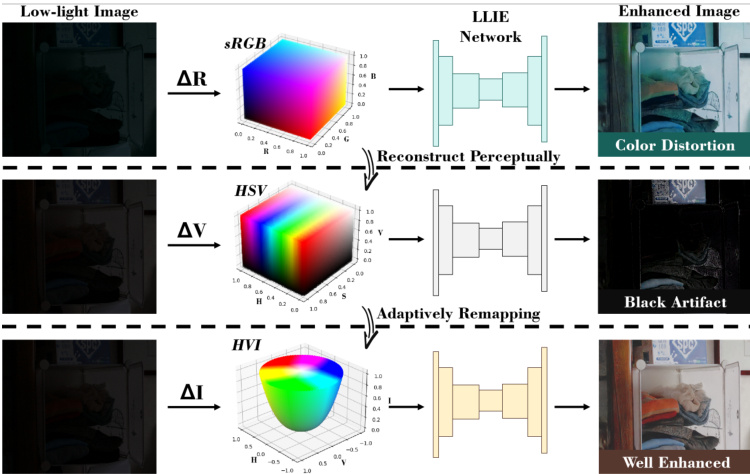
Fig. 1: The sensitivity comparison of different color spaces in lowlight enhancement. The notations $\Delta{\sf R}$ , $\Delta\mathrm{V}_{:}$ , and $\Delta\mathbf{I}$ represent a tiny variation in the axis of Red (sRGB), Value (HSV), and Intensity (HVI), respectively. After enhancement processing, noticeable color artifacts can be observed in the sRGB and HSV space results.
图 1: 不同色彩空间在低光照增强中的敏感性对比。符号$\Delta{\sf R}$、$\Delta\mathrm{V}_{:}$和$\Delta\mathbf{I}$分别表示红轴(sRGB)、明度轴(HSV)和强度轴(HVI)的微小变化。经过增强处理后,在sRGB和HSV空间结果中可观察到明显的色彩伪影。
While the HSV color space [8] enables the separation of brightness and color of the image from sRGB channels, the discontinuous property of hue axis (see Sec. III-B) and its intricate mapping relationships with sRGB space makes it challenging to handle complex and varying lighting conditions. As shown in Fig. 1, enhanced images with the HSV space often have obvious black artifacts due to extremely low light environments. We consider that the color space (e.g., sRGB, HSV) has a huge impact on the image enhancement effect.
虽然HSV色彩空间[8]能够将图像的亮度和颜色从sRGB通道中分离出来,但色相轴的不连续性(见第III-B节)及其与sRGB空间复杂的映射关系,使得处理复杂多变的照明条件具有挑战性。如图1所示,在极低光环境下,使用HSV空间增强的图像常会出现明显的黑色伪影。我们认为色彩空间(如sRGB、HSV)对图像增强效果有重大影响。
To address the aforementioned issue between the low-light image enhancement task and existing color spaces, we introduce a new color space named Horizontal/Vertical-Intensity (HVI), designed specifically to cater to the needs of lowlight enhancement tasks. The proposed HVI color space not only decouples brightness and color information but also incorporates three trainable representation parameters and a trainable function, allowing it to adapt to the brightening scale and color variations of different low-light images. Building upon the HVI color space, to fully leverage the decoupled information, we propose a new LLIE method, named Color and Intensity Decoupling Network (CIDNet). CIDNet consists of HV-branch and intensity-branch, which makes full use of decoupled information to generate high-quality results. After applying the HVI transformation to the image, it is separately fed into the HV-branch to extract color information, and the intensity-branch to establish the photometric mapping function under different lighting conditions. Additionally, to enhance the interaction between the structures of images contained in the brightness and color branches, we propose the bidirectional Lighten Cross-Attention (LCA) module to learn the complementary information of HV-branch and intensity-branch. Furthermore, we conduct experiments and ablation studies on multiple datasets to validate our approach. The experimental results demonstrate that CIDNet effectively enhances the brightness of low-light images while preserving their natural colors, which validates the compatibility of the proposed HVI color space with low-light image enhancement tasks. Note that the proposed method exhibits relatively small parameters (1.88M) and computational loads (7.57G), achieving a good balance between effectiveness and efficiency on edge devices. Our contributions can be summarized as follows:
为解决低光照图像增强任务与现有色彩空间之间的上述问题,我们提出了一种名为水平/垂直-亮度(HVI)的新型色彩空间,专为满足低光照增强任务需求而设计。所提出的HVI色彩空间不仅能解耦亮度和色彩信息,还包含三个可训练表示参数和一个可训练函数,使其能适应不同低光照图像的亮度尺度与色彩变化。基于HVI色彩空间,为充分利用解耦信息,我们提出了一种新的低光照图像增强方法——色彩与亮度解耦网络(CIDNet)。CIDNet由HV分支和亮度分支组成,通过充分运用解耦信息生成高质量结果。图像经HVI转换后,分别输入HV分支提取色彩信息,以及亮度分支建立不同光照条件下的光度映射函数。此外,为增强亮度与色彩分支所含图像结构间的交互,我们提出了双向光照交叉注意力(LCA)模块来学习HV分支与亮度分支的互补信息。我们在多个数据集上进行了实验与消融研究以验证方法有效性。实验结果表明,CIDNet在提升低光照图像亮度的同时能保持自然色彩,验证了HVI色彩空间与低光照增强任务的兼容性。值得注意的是,该方法参数量(1.88M)和计算量(7.57G)相对较小,在边缘设备上实现了效果与效率的良好平衡。我们的贡献可总结如下:
II. RELATED WORK
II. 相关工作
A. Low-Light Image Enhancement
A. 低光照图像增强
Traditional and Plain LLIE Methods. Plain methods usually enhanced image by histogram equalization [9] and Gama Corrction [10]. Traditional method [11] commonly depends on the application of the Retinex theory, which decomposes the lights into illumination and reflections. For example, Guo et al. [12] refine the initial illumination map to optimize lighting details by imposing a structure prior. Regrettably, existing methodologies are inadequate in effectively eliminating noise artifacts and producing accurate color mappings, rendering them incapable of achieving the desired level of precision and finesse in the LLIE tasks.
传统与朴素低光照图像增强方法。朴素方法通常通过直方图均衡化[9]和伽马校正[10]来增强图像。传统方法[11]普遍基于Retinex理论,将光线分解为照度与反射分量。例如Guo等[12]通过引入结构先验来优化初始照度图以提升光照细节。遗憾的是,现有方法在有效消除噪声伪影和生成精确色彩映射方面存在不足,导致其无法达到低光照增强任务所需的精度与细腻度。
Deep Learning Methods. Deep learning-based approaches [2], [3], [13], [14] has been widely used in LLIE task. Existing methods propose distinct solutions to address the issues of image color shift and noise stabilization. For instance, RetinexNet [6] enhances images by decoupling illumination and reflectance based on Retinex theory. However, it has unsatisfied results with several color shifts. SNR-Aware [15] presents a collectively exploiting Signal-to-Noise-Ratioaware transformers to dynamically enhance pixels with spatialvarying operations, which could reduce the color bias and noise. Bread [8] decouples the entanglement of noise and color distortion by using YCbCr color space. Furthermore, they designed a color adaption network to tackle the color distortion issue left in light-enhanced images. Still, SNRAware and Bread show poor generalization ability. They are not only inaccurately controlled in terms of brightness in some of the datasets, but also biased in terms of color with pure black area.
深度学习方法。基于深度学习的方法 [2]、[3]、[13]、[14] 已被广泛应用于低光照图像增强 (LLIE) 任务。现有方法针对图像色偏和噪声稳定问题提出了不同解决方案。例如,RetinexNet [6] 基于Retinex理论通过解耦光照与反射率来增强图像,但存在明显色偏问题。SNR-Aware [15] 提出利用信噪比感知 (Signal-to-Noise-Ratioaware) Transformer 动态执行空间可变像素增强,可减少色彩偏差和噪声。Bread [8] 通过YCbCr色彩空间解耦噪声与色彩失真,并设计色彩适应网络处理增强图像的残留色偏问题。然而SNR-Aware和Bread的泛化能力较差,不仅在部分数据集中存在亮度控制失准问题,对纯黑区域还会产生色彩偏差。
Diffusion Model-based Methods. With the advancement of Denoising Diffusion Probabilistic Models (DDPMs) [16], diffusion-based generative models have achieved remarkable results in the LLIE task. It has indeed shown the capability to generate more accurate and appropriate images in pure black spaces devoid of information and under low light conditions with significant noise. However, they still exhibit issues such as local overexposure or color shift. Recent LLIE diffusion methods have attempted to address these challenges by incorporating global supervised brightness correction or employing local color correctors [17]–[19]. PyDiff [17] employs a Global Feature Modulation to correct the pixel noise and color bias globally. Diff-Retinex [20] rethink the retinex theory with a diffusion-based model in the LLIE task, which decomposed an image to illumination and reflectance colors to reduce color bias and enhance brightness separately. However, the aforementioned diffusion models suffer from long training and inference times, lack of Lighten efficiency, and inability to fully decouple brightness and color information.
基于扩散模型的方法。随着去噪扩散概率模型 (Denoising Diffusion Probabilistic Models, DDPM) [16] 的发展,基于扩散的生成模型在低光照图像增强 (LLIE) 任务中取得了显著成果。该模型确实展现了在纯黑无信息空间及强噪声低光条件下生成更准确、更合适图像的能力,但仍存在局部过曝或色偏等问题。近期基于扩散的LLIE方法尝试通过引入全局监督亮度校正或采用局部色彩校正器 [17]–[19] 来解决这些挑战。PyDiff [17] 采用全局特征调制 (Global Feature Modulation) 来全局校正像素噪声和色彩偏差。Diff-Retinex [20] 在LLIE任务中以扩散模型重新思考Retinex理论,将图像分解为光照分量和反射分量以分别降低色偏并增强亮度。然而上述扩散模型仍存在训练推理耗时长、提亮效率不足、无法完全解耦亮度与色彩信息等缺陷。
B. Color Space
B. 色彩空间
RGB. Currently, the most commonly used is the standardRGB (sRGB) color space. For the same principle as visual recognition by the human eye, sRGB is widely used in digital imaging devices [21]. Nevertheless, image brightness and color exhibit a strong interdependence with the three channels in sRGB. A slight disturbance in the color space will cause an obvious variation in both the brightness and color of the generated image. Thus, sRGB is not the optimal color space for enhancement.
RGB。目前最常用的是标准RGB (sRGB) 色彩空间。由于与人眼视觉识别原理相同,sRGB被广泛应用于数字成像设备 [21]。然而,在sRGB中图像亮度与色彩三个通道存在强关联性,色彩空间的轻微扰动会导致生成图像的亮度和色彩发生明显变化。因此,sRGB并非图像增强的最佳色彩空间。
HSV and YCbCr. Hue, Saturation and Value (HSV) color space represents points in an RGB color model with a cylindrical coordinate system [22]. Indeed, it does decouple brightness and color of the image from RGB channels. However, the inherent hue axis color discontinuity and non-mono-mapped pure black planes pose significant challenges when attempting to enhance the image in HSV color space, resulting in the emergence of obvious artifacts. To circumvent issues related to HSV, some methods [8], [23] also transform sRGB images to the YCbCr color space for processing, which has an illumination axis (Y) and reflect-color-plain (CbCr). Although it solved the hue dimension discontinuity problem of HSV, the multi-mapping of pure black planes still exists.
HSV 和 YCbCr。色调、饱和度和明度 (HSV) 色彩空间通过柱坐标系表示 RGB 色彩模型中的点 [22]。它确实将图像的亮度和颜色与 RGB 通道解耦,但其固有的色调轴颜色不连续性及非单映射纯黑平面在 HSV 色彩空间中进行图像增强时会带来显著挑战,导致明显伪影的出现。为避免 HSV 相关问题,部分方法 [8][23] 也会将 sRGB 图像转换至 YCbCr 色彩空间处理,该空间包含亮度轴 (Y) 和反射色平面 (CbCr)。尽管它解决了 HSV 的色调维度不连续问题,但纯黑平面的多重映射现象仍然存在。
III. HVI COLOR SPACE
III. HVI 色彩空间
To address the misalignment between LLIE and existing color spaces, we innovative ly introduce a trainable color space in the field of LLIE, named Horizontal/Vertical-Intensity (HVI) color space. HVI color space consists of three trainable parameters and a custom training function that can adapt to the photosensitive characteristics and color sensitivities of lowlight images. In this section, we will present the description of the mono-mapping image transformation from sRGB space to HVI color space, as well as the details of HVI color space.
为解决低光照图像增强(LLIE)与现有色彩空间不匹配的问题,我们创新性地在LLIE领域引入了一种可训练的色彩空间,命名为水平/垂直-强度(HVI)色彩空间。HVI色彩空间由三个可训练参数和一个自定义训练函数组成,能够适应低光照图像的光敏特性和色彩敏感度。本节将详细介绍从sRGB空间到HVI色彩空间的单映射图像转换方法,以及HVI色彩空间的具体细节。
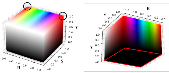
Fig. 2: HSV color space visualization. The two black circles in the left image indicate the discontinuous color positions along the hue axis, while the red box in the right image displays a pure black plane with Value $=0$ .
图 2: HSV色彩空间可视化。左图中的两个黑色圆圈表示沿色调轴的不连续颜色位置,而右图中的红色框显示了一个纯黑色平面,其亮度值 $=0$。
A. Intensity Map
A. 强度图
In the task of LLIE, one crucial aspect is accurately estimating the illumination intensity map of the scene. Following retinex-based LLIE methods [6], [7], [12], we represent the intensity map of an image with the maximum value among the RGB channels. According to the definition, we can calculate the intensity map of an image $\mathbf{I}_{m a x}\in\mathbb{R}^{\mathrm{H}\times\mathrm{W}\times3}$ as follows:
在LLIE任务中,一个关键环节是准确估计场景的照明强度图。基于Retinex理论的LLIE方法[6][7][12],我们使用RGB通道中的最大值来表示图像的强度图。根据定义,图像强度图$\mathbf{I}_{m a x}\in\mathbb{R}^{\mathrm{H}\times\mathrm{W}\times3}$的计算方式如下:
$$
\mathbf{I}{m a x}=\operatorname*{max}{\mathbf{c}\in{R,G,B}}(\mathbf{I_{c}}),
$$
$$
\mathbf{I}{m a x}=\operatorname*{max}{\mathbf{c}\in{R,G,B}}(\mathbf{I_{c}}),
$$
Next, we will introduce how to utilize the intensity map to guide the generation of the corresponding HV color map.
接下来,我们将介绍如何利用强度图来指导生成相应的HV彩色图。
B. HV Transformation
B. HV 变换
To effectively address color deviations, previous LLIE methods typically separate an sRGB image into a reflectance map [2], [6] based on the retinex theory. These approaches often require a large computational network for fitting, which need to use a combination of hue and saturation to simulate the reflectance map. However, the HSV color space is discontinued in the hue axis (see the black circles in Fig. 2) and has a non-bijection pure black plane (see the red rectangle in Fig. 2), which disrupts the one-to-one mapping. For discontinuity of the hue axis, based on HSV color transform formula, a red color in sRGB $(R,G,B)=(1,0,0)$ corresponds to $(0,1,1)$ and $(1,1,1)$ in HSV color space. For the pure black plane, as shown in Fig. 2, any HSV pixel with Value $=~0$ denote the black color, corresponding to $(R,G,B)=(0,0,0)$ in sRGB color space. Thus, the one-to-many mapping is the source reason of why the existing methods on HSV color space generate the obvious artifacts in the dark regions.
为有效解决色彩偏差问题,现有LLIE方法通常基于视网膜反射理论将sRGB图像分解为反射率图[2][6]。这类方法往往需要庞大的计算网络进行拟合,需结合色调与饱和度来模拟反射率图。然而HSV色彩空间的色调轴存在不连续性(见图2中黑色圆圈),且存在非双射的纯黑平面(见图2中红色矩形),破坏了一对一映射关系。针对色调轴不连续性问题,根据HSV色彩转换公式,sRGB中的红色$(R,G,B)=(1,0,0)$对应HSV色彩空间中的$(0,1,1)$和$(1,1,1)$;对于纯黑平面,如图2所示,任何Value$=~0$的HSV像素均表示黑色,对应sRGB色彩空间的$(R,G,B)=(0,0,0)$。这种一对多映射关系正是现有HSV色彩空间方法在暗区产生明显伪影的根本原因。
To address the suboptimum problems caused by one-tomany mapping (HSV color space), we design a trainable Horizonal/Vertical (HV) color map as a plane to quantify a color-reflectance map, which is a one-to-one mapping to sRGB color space. The HVI color space consists of three trainable parameters $k$ , $\gamma_{G}$ and $\gamma_{B}$ , and a custom training function $T(x)$ .
为了解决一对多映射(HSV色彩空间)导致的次优问题,我们设计了一个可训练的横向/纵向(HV)色彩映射平面来量化色彩-反射率映射,该平面与sRGB色彩空间形成一对一映射关系。HVI色彩空间包含三个可训练参数$k$、$\gamma_{G}$和$\gamma_{B}$,以及一个自定义训练函数$T(x)$。
Parameter $k$ . Considering that the dark regions of lowlight images have small values, which is hard to distinguish the color and causes information loss. Based on the proposed HVI color space, we customize a parameter $k$ that allows networks to adjust the color point density of the low-intensity color plane, which quantifies a Color-Density $k$ $\left(\mathbf{C}_{k}\right)$ as
参数 $k$。考虑到低光图像的暗区数值较小,难以区分颜色并导致信息丢失。基于提出的HVI色彩空间,我们定制了一个参数 $k$,使网络能够调整低强度色彩平面的色点密度,并将其量化为色彩密度 $k$ $\left(\mathbf{C}_{k}\right)$。
$$
\mathbf{C}{k}=\sqrt[k]{\sin(\frac{\pi\mathbf{I}_{m a x}}{2})+\varepsilon},
$$
$$
\mathbf{C}{k}=\sqrt[k]{\sin(\frac{\pi\mathbf{I}_{m a x}}{2})+\varepsilon},
$$
where $k\in\mathbb{Q}^{+}$ and we set $\varepsilon=1\times10^{-8}$ .
其中 $k\in\mathbb{Q}^{+}$ 且设 $\varepsilon=1\times10^{-8}$。
Hue bias parameter $\gamma_{G}$ and $\gamma_{B}$ . Since different cameras have different sensitivity on RGB channel, it will cause color shift (i.e. green color) on the low-light scenes. To alleviate the data diversity caused by color shift, we learn an adaptive linear Color-Perceptual map $\mathbf{P}_{\gamma}$ on hue value.
色调偏差参数 $\gamma_{G}$ 和 $\gamma_{B}$。由于不同相机对RGB通道的敏感度不同,会导致低光场景出现色彩偏移(如偏绿色)。为缓解色彩偏移造成的数据多样性,我们在色调值上学习了一个自适应线性色彩感知映射 $\mathbf{P}_{\gamma}$。
where $\gamma_{G},\gamma_{B}\in(0,1)$ , $\mathbf{H}\in[0,1]$ denotes the hue value.
其中 $\gamma_{G},\gamma_{B}\in(0,1)$ , $\mathbf{H}\in[0,1]$ 表示色调值。
Customizable or trainable function $T(x)$ . To improve the saturation the generated results, we design a Function-Density $T$ based on the $\mathbf{P}_{\gamma}$ to adaptively adjust the saturation. We utilize a Function-Density $T$ as
可定制或可训练函数 $T(x)$ 。为了提升生成结果的饱和度,我们基于 $\mathbf{P}_{\gamma}$ 设计了一个函数密度 $T$ 来自适应调整饱和度。具体采用函数密度 $T$ 的形式为
$$
\begin{array}{r}{\mathbf{D}{T}=T(\mathbf{P}_{\gamma}),}\end{array}
$$
$$
\begin{array}{r}{\mathbf{D}{T}=T(\mathbf{P}_{\gamma}),}\end{array}
$$
where $T(\cdot)$ satisfies $T(0)=T(1)$ and $T(\mathbf{P}_{\gamma})\geq0$ . Finally, we formalize the horizontal $(\hat{\mathbf{H}})$ and vertical $(\hat{\mathbf{V}})$ plane as
其中 $T(\cdot)$ 满足 $T(0)=T(1)$ 且 $T(\mathbf{P}_{\gamma})\geq0$。最终,我们将水平面 $(\hat{\mathbf{H}})$ 和垂直面 $(\hat{\mathbf{V}})$ 形式化为
$$
\begin{array}{r}{\hat{\mathbf{H}}=\mathbf{C}{k}\odot\mathbf{S}\odot\mathbf{D}{T}\odot h,}\ {\hat{\mathbf{V}}=\mathbf{C}{k}\odot\mathbf{S}\odot\mathbf{D}_{T}\odot v,}\end{array}
$$
$$
\begin{array}{r}{\hat{\mathbf{H}}=\mathbf{C}{k}\odot\mathbf{S}\odot\mathbf{D}{T}\odot h,}\ {\hat{\mathbf{V}}=\mathbf{C}{k}\odot\mathbf{S}\odot\mathbf{D}_{T}\odot v,}\end{array}
$$
where $\odot$ denotes the element-wise multiplication. Note that we orthogonal ize our color map by setting an intermediate variable $h=\cos(2\pi\mathbf{P}{\gamma})$ and $v=\sin(2\pi\mathbf{P}_{\gamma})$ to be bijective.
其中 $\odot$ 表示逐元素相乘。注意,我们通过设置中间变量 $h=\cos(2\pi\mathbf{P}{\gamma})$ 和 $v=\sin(2\pi\mathbf{P}_{\gamma})$ 使颜色映射双射正交化。
C. Perceptual-invert HVI Transformation
C. 感知可逆的HVI变换
To convert HVI back to the HSV color space, we design a Perceptual-invert HVI Transformation (PHVIT), which is a surjective mapping while allowing for the independent adjustment of the image’s saturation and brightness.
为了将HVI转换回HSV色彩空间,我们设计了一种感知可逆的HVI变换(PHVIT),这是一种满射映射,同时允许独立调整图像的饱和度和亮度。
To transform injective ly, the PHVIT sets $\hat{h}$ and $\hat{v}$ as an intermediate variable as
为了进行单射变换,PHVIT将$\hat{h}$和$\hat{v}$设为中间变量
$$
\hat{h}=\frac{\hat{\mathbf{I}}{\mathbf{H}}}{\mathbf{D}{T}\mathbf{C}{k}+\varepsilon},\hat{v}=\frac{\hat{\mathbf{I}}{\mathbf{V}}}{\mathbf{D}{T}\mathbf{C}_{k}+\varepsilon},
$$
$$
\hat{h}=\frac{\hat{\mathbf{I}}{\mathbf{H}}}{\mathbf{D}{T}\mathbf{C}{k}+\varepsilon},\hat{v}=\frac{\hat{\mathbf{I}}{\mathbf{V}}}{\mathbf{D}{T}\mathbf{C}_{k}+\varepsilon},
$$
where $\varepsilon=1\times10^{-8}$ . Then, we convert $\hat{h}$ and $\hat{v}$ to HSV color space. The hue map can be formulated by
其中 $\varepsilon=1\times10^{-8}$。接着,我们将 $\hat{h}$ 和 $\hat{v}$ 转换到 HSV 色彩空间。色调图可通过以下公式表示:
$$
H=F_{\gamma}(\arctan(\frac{\hat{v}}{\hat{h}})\mod1),
$$
$$
H=F_{\gamma}(\arctan(\frac{\hat{v}}{\hat{h}})\mod1),
$$
where $F_{\gamma}$ is a inverse linear function as
其中 $F_{\gamma}$ 是一个反线性函数,形式为
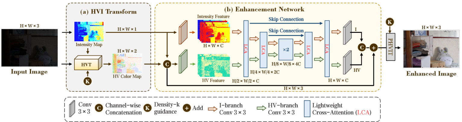
Fig. 3: The overview of the proposed CIDNet. (a) HVI Color Transformation (HVIT) takes an sRGB image as input and generates HV color map and intensity map as outputs. (b) Enhancement Network performs the main processing, utilizing a dual-branch UNet architecture, which contains six Lighten Cross-Attention (LCA) blocks. Lastly, we apply Perceptual-inverse HVI Transform (PHVIT) to take a light-up HVI map as input and transform it into an sRGB-enhanced image.
图 3: 提出的CIDNet框架概览。(a) HVI色彩变换(HVIT)以sRGB图像作为输入,生成HV色彩图和亮度图作为输出。(b) 增强网络采用双分支UNet架构进行核心处理,包含六个轻量化交叉注意力(LCA)模块。最后通过感知逆HVI变换(PHVIT)将提亮后的HVI映射转换为增强的sRGB图像。
where $\gamma_{G},\gamma_{B}$ are mentioned in Eq. 3. The saturation and value map can be perceptual ly estimated as
其中 $\gamma_{G},\gamma_{B}$ 在公式3中已提及。饱和度和明度图可通过感知方式估算为
$$
\begin{array}{l}{{S=\alpha_{S}\sqrt{\hat{h}^{2}+\hat{v}^{2}},}}\ {{V=\alpha_{I}\hat{\bf I}_{\bf I},}}\end{array}
$$
$$
\begin{array}{l}{{S=\alpha_{S}\sqrt{\hat{h}^{2}+\hat{v}^{2}},}}\ {{V=\alpha_{I}\hat{\bf I}_{\bf I},}}\end{array}
$$
where $\alpha_{s},\alpha_{i}$ are the customizing linear parameters to change the image color saturation and brightness. Finally, we will obtain the sRGB image with HSV image [22].
其中 $\alpha_{s},\alpha_{i}$ 是用于调整图像色彩饱和度(saturation)和亮度(brightness)的自定义线性参数。最终我们将获得带有HSV图像[22]的sRGB图像。
IV. CIDNET
IV. CIDNET
Based on the proposed HVI space, we introduce a novel dual-branch LLIE network, named the Color and Intensity Decoupling Network (CIDNet) to separately address HV-plain and I-axis information in the HVI space. The CIDNet employs HV-branch to suppress the noise and chromatic it y in the dark regions and utilizes I-branch to estimate the luminance of the whole images. Furthermore, we design an Lighten CrossAttention (LCA) module to facilitate interaction guidance between the HV-branch and I-branch. In this section, we provide a detailed description of the architecture of CIDNet.
基于提出的HVI空间,我们引入了一种新颖的双分支低光照图像增强网络,称为色彩与亮度解耦网络(CIDNet),用于分别处理HVI空间中的HV平面和I轴信息。CIDNet采用HV分支抑制暗区的噪声和色度,利用I分支估计整幅图像的亮度。此外,我们设计了轻量交叉注意力(LCA)模块来促进HV分支与I分支之间的交互引导。本节将详细描述CIDNet的网络架构。
A. Pipeline
A. 流水线
As shown in Fig. 3, the overall framework can be divided into three consecutive main steps, i.e., HVI transformation, enhancement network, and perceptual-inverse HVI transformation.
如图 3 所示,整体框架可分为三个连续的主要步骤,即 HVI 转换、增强网络和感知逆 HVI 转换。
As described in Sec. III, the HVI transformation decomposes the sRGB image into two components: an intensity map containing scene ill umi nance information and an HV color map containing scene color and structure information. Specifically, we first calculate the intensity map using Eq. 1, which is ${\mathbf{I}}{\mathbf{I}}={\mathbf{I}}_{m a x}$ . Subsequently, we utilize the intensity map and the original image to generate HV color map using Eq. 5. Furthermore, a trainable density $k$ is employed to adjust the color point density of the low-intensity color plane, as shown in Fig. 3(a).
如第 III 节所述,HVI 变换将 sRGB 图像分解为两个分量:包含场景照度信息的强度图 (intensity map) 和包含场景颜色与结构信息的 HV 色彩图 (HV color map)。具体而言,我们首先通过公式 1 计算强度图 ${\mathbf{I}}{\mathbf{I}}={\mathbf{I}}_{m a x}$,随后利用强度图和原始图像通过公式 5 生成 HV 色彩图。此外,如图 3(a) 所示,我们采用可训练密度参数 $k$ 来调节低强度色彩平面的色点密度。
Based on the UNet architecture, the enhancement network takes an intensity map and HV color map as input. To learn the initial information of intensity map and HV color map, we employ $3\times3$ convolutional layers to obtain the features with same dimension in each branch. Subsequently, the features are fed into the UNet with Lighten Cross-Attention (LCA) modules. The LCA module consists of cross attention blocks, color denoise layer and intensity enhance layer. The cross attention block learns the corresponding interacted information between the HV-branch and I-branch. The color denoise layer avoids noise artifacts and color shift, and the intensity enhance layer improves the luminance and removes the saturated regions. The final outputs of UNet are the refined intensity and HV maps. To decrease the difficulty of the learning process, we employ a residual mechanism to add the original HVI map. Finally, we perform an HVI inverse transformation with the trainable parameter density $k$ to map the image to the sRGB space.
基于UNet架构的增强网络以强度图和HV彩色图作为输入。为学习强度图和HV彩色图的初始信息,我们采用$3\times3$卷积层在各分支中获取相同维度的特征。随后,这些特征被输入带有轻量交叉注意力(LCA)模块的UNet网络。LCA模块由交叉注意力块、色彩降噪层和强度增强层组成:交叉注意力块学习HV分支与I分支间的交互信息;色彩降噪层避免噪声伪影和色偏;强度增强层提升亮度并消除饱和区域。UNet的最终输出是优化后的强度图和HV图。为降低学习难度,我们采用残差机制叠加原始HVI图。最后通过可训练参数密度$k$进行HVI逆变换,将图像映射至sRGB色彩空间。
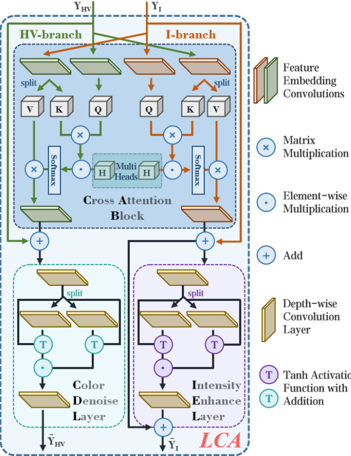
Fig. 4: The dual-branch Lighten Cross-Attention (LCA) block (i.e., I-branch and HV-branch). The LCA incorporates a Cross Attention Block (CAB), an Intensity Enhance Layer (IEL), and a Color Denoise Layer (CDL). The feature embedding convolution layers contains a $1\times1$ depth-wise convolution and a $3\times3$ group convolution.
图 4: 双分支轻量化交叉注意力 (LCA) 模块 (即 I 分支和 HV 分支)。该模块包含交叉注意力块 (CAB)、强度增强层 (IEL) 和色彩降噪层 (CDL)。特征嵌入卷积层由 $1\times1$ 深度可分离卷积和 $3\times3$ 分组卷积构成。
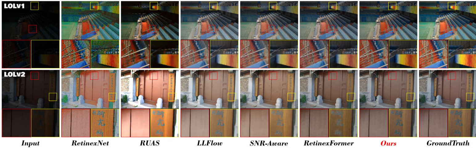
Fig. 5: Visual comparisons of the enhanced results by different methods on LOLv1 and LOLv2. (Zoom in for the best view.)
图 5: 不同方法在 LOLv1 和 LOLv2 数据集上的增强效果视觉对比。(建议放大查看最佳效果)
B. Structure
B. 结构
- Enhancement Network: As depicted in Fig. 3(b), we use the commonly employed UNet as the baseline network, which has an encoder, decoder, and multiple skip connections. The encoder includes three LCA blocks and downsample and $3\times3$ kernel convolutional layers. Similarly, the decoder consists of three LCA modules, and upsampling layers.
- 增强网络:如图 3(b) 所示,我们采用常用的 UNet 作为基线网络,该网络包含编码器、解码器和多个跳跃连接。编码器包含三个 LCA 块、下采样层和 $3\times3$ 核卷积层。类似地,解码器由三个 LCA 模块和上采样层构成。
- Lighten Cross-Attention: To enhance the interaction between the structures of images contained in the brightness and color branches, we propose the Lighten Cross-Attention (LCA) module to learn the complementary information of HV-branch and intensity-branch. As shown in Fig. 4, the HV-branch and I-branch in LCA handle HV features and intensity features, respectively. To learn the complementary potential between HV features and intensity features during the processing, we propose cross attention block (CAB) to facilitate mutual guidance between HV features and intensity features. To force the CAB to learn the information from the opposite branch (i.e., HV branch only use the information of I-brach to refine itself), we utilize the one branch as the query and leverage another branch as key and value in the CAB.
- Lighten Cross-Attention:为增强亮度分支与色彩分支中图像结构的交互,我们提出Lighten Cross-Attention (LCA) 模块来学习HV分支与强度分支的互补信息。如图4所示,LCA中的HV分支和I分支分别处理HV特征与强度特征。为在学习过程中挖掘HV特征与强度特征的互补潜力,我们提出交叉注意力块 (CAB) 来促进两种特征间的相互引导。为确保CAB仅从对立分支学习信息 (即HV分支仅利用I分支信息优化自身),我们在CAB中将一个分支作为query,另一个分支作为key和value。
As shown in 4, The CAB exhibits a symmetrical structure between the I-way and HV-way. We use the I-branch as an example to describe the details. $\mathbf{Y_{I}}\in\mathbb{R}^{\hat{H}\times\hat{W}\times\hat{C}}$ denotes the inputs of I-branch, our CAB first derives query $\mathbf{\Psi}^{(\mathbf{Q})}$ by $\mathbf{Q}=$ $W^{(Q)}\mathbf{Y_{I}}$ . Meanwhile, the CAB splits key $(\mathbf{K})$ and value $(\mathbf{V})$ by $\mathbf{K}=W^{(K)}\mathbf{Y_{I}}$ and $\mathbf{V} =~{\bar{W}}^{(V)}\mathbf{Y_{I}}$ . $W^{(Q)}$ , $W^{(K)}$ and $\dot{W}^{(V)}$ represents the feature embedding convolution layers. We formulate as
如图4所示,CAB在I-way和HV-way之间呈现出对称结构。我们以I-branch为例说明细节。$\mathbf{Y_{I}}\in\mathbb{R}^{\hat{H}\times\hat{W}\times\hat{C}}$表示I-branch的输入,我们的CAB首先通过$\mathbf{Q}=$$W^{(Q)}\mathbf{Y_{I}}$生成查询$\mathbf{\Psi}^{(\mathbf{Q})}$。同时,CAB通过$\mathbf{K}=W^{(K)}\mathbf{Y_{I}}$和$\mathbf{V} =~{\bar{W}}^{(V)}\mathbf{Y_{I}}$拆分键$(\mathbf{K})$与值$(\mathbf{V})$。$W^{(Q)}$、$W^{(K)}$和$\dot{W}^{(V)}$代表特征嵌入卷积层。我们将其表述为
$$
{\hat{\mathbf{Y}}}{\mathbf{I}}=W(\mathbf{V}\otimes\operatorname{Softmax}\left(\mathbf{Q}\otimes\mathbf{K}/\alpha_{H}\right)+\mathbf{Y}_{\mathbf{I}})
$$
$$
{\hat{\mathbf{Y}}}{\mathbf{I}}=W(\mathbf{V}\otimes\operatorname{Softmax}\left(\mathbf{Q}\otimes\mathbf{K}/\alpha_{H}\right)+\mathbf{Y}_{\mathbf{I}})
$$
where $\alpha_{H}$ is the multi-head factor [24] and $W(\cdot)$ denotes the feature embedding convolutions.
其中 $\alpha_{H}$ 是多头因子 [24],$W(\cdot)$ 表示特征嵌入卷积。
Next, following Retinex theory, intensity enhance layer (IEL) decomposes the tensor $\hat{\mathbf{Y_{I}}}$ as $\mathbf{Y}{I}{\dot{\mathbf{\theta}}}=\mathbf{\theta}W^{(I)}{\hat{\mathbf{Y}}}{\mathbf{I}}$ and $\mathbf{Y}{R}=W^{(R)}\bar{\hat{\mathbf{Y}}}_{\mathbf{I}}$ . The IEL is defined as
接下来,根据Retinex理论,强度增强层(IEL)将张量$\hat{\mathbf{Y_{I}}}$分解为$\mathbf{Y}{I}{\dot{\mathbf{\theta}}}=\mathbf{\theta}W^{(I)}{\hat{\mathbf{Y}}}{\mathbf{I}}$和$\mathbf{Y}{R}=W^{(R)}\bar{\hat{\mathbf{Y}}}_{\mathbf{I}}$。IEL定义为
$$
\begin{array}{r}{\tilde{\mathbf{Y}}{\mathbf{I}}=W_{s}((\operatorname{tanh}{(W_{s}\mathbf{Y}{I})}+\mathbf{Y}{I})\quad}\ {\odot(\operatorname{tanh}{(W_{s}\mathbf{Y}{R})}+\mathbf{Y}_{R}))}\end{array}
$$
$$
\begin{array}{r}{\tilde{\mathbf{Y}}{\mathbf{I}}=W_{s}((\operatorname{tanh}{(W_{s}\mathbf{Y}{I})}+\mathbf{Y}{I})\quad}\ {\odot(\operatorname{tanh}{(W_{s}\mathbf{Y}{R})}+\mathbf{Y}_{R}))}\end{array}
$$
where $\odot$ represents the element-wise multiplication and $W_{s}$ denotes the depth-wise convolution layers. Finally, the output of IEL adds the residuals to simplify the training process.
其中 $\odot$ 表示逐元素相乘,$W_{s}$ 表示深度卷积层。最终,IEL (Intra-Encoder Layer) 的输出通过添加残差来简化训练过程。
C. Loss Function
C. 损失函数
To integrate the advantages of HVI space and the sRGB space, the loss function consists both color spaces. In HVI color space, we utilize L1 loss $L_{1}$ , edge loss $L_{e}$ [25], and perceptual loss $L_{p}$ [26] for the low-light enhancement task. It can be expressed as
为了整合HVI空间和sRGB空间的优势,损失函数同时包含这两个色彩空间。在HVI色彩空间中,我们采用L1损失$L_{1}$、边缘损失$L_{e}$[25]以及感知损失$L_{p}$[26]来完成低光增强任务。其表达式为
$$
\begin{array}{r}{l(\hat{X}{H V I},X_{H V I})=\lambda_{1}\cdot L_{1}(\hat{X}{H V I},X_{H V I})}\ {+\lambda_{e}\cdot L_{e}(\hat{X}{H V I},X_{H V I}),}\ {+\lambda_{p}\cdot L_{p}(\hat{X}{H V I},X_{H V I})}\end{array}
$$
$$
\begin{array}{r}{l(\hat{X}{H V I},X_{H V I})=\lambda_{1}\cdot L_{1}(\hat{X}{H V I},X_{H V I})}\ {+\lambda_{e}\cdot L_{e}(\hat{X}{H V I},X_{H V I}),}\ {+\lambda_{p}\cdot L_{p}(\hat{X}{H V I},X_{H V I})}\end{array}
$$
where $\lambda_{1},\lambda_{e},\lambda_{p}$ are all the weight to trade-off the loss function $l(\cdot)$ . In sRGB color space, we employ the same loss function as $l(\hat{I},I)$ . Therefore, our overall loss function $L$ is represented by
其中 $\lambda_{1},\lambda_{e},\lambda_{p}$ 均为权衡损失函数 $l(\cdot)$ 的权重。在 sRGB 色彩空间中,我们采用与 $l(\hat{I},I)$ 相同的损失函数。因此,我们的总体损失函数 $L$ 可表示为
$$
\boldsymbol{L}=\lambda_{c}\cdot\boldsymbol{l}(\hat{\mathbf{I}}{\mathbf{HVI}},\mathbf{I}_{\mathbf{HVI}})+\boldsymbol{l}(\hat{\mathbf{I}},\mathbf{I})
$$
$$
\boldsymbol{L}=\lambda_{c}\cdot\boldsymbol{l}(\hat{\mathbf{I}}{\mathbf{HVI}},\mathbf{I}_{\mathbf{HVI}})+\boldsymbol{l}(\hat{\mathbf{I}},\mathbf{I})
$$
where $\lambda_{c}$ is the weight to balance the loss in different color spaces.
其中 $\lambda_{c}$ 是用于平衡不同色彩空间中损失的权重。
V. EXPERIMENTS
V. 实验
A. Datasets and Settings
A. 数据集与设置
We employ seven commonly-used LLIE benchmark datasets for evaluation, including LOLv1 [6], LOLv2 [27], DICM [28], LIME [12], MEF [29], NPE [30], and VV [31]. We also conduct further experiments on two extreme datasets, SICE [32] (containing mix and grad test sets [33]) and SID (SonyTotal-Dark) [34]. Since blurring is often prone to occur in low-luminosity images, to demonstrate the robustness of our CIDNet to multitasking, we conducted experiments on LOLBlur [35] as well.
我们采用七个常用低光照图像增强(LLIE)基准数据集进行评估,包括LOLv1 [6]、LOLv2 [27]、DICM [28]、LIME [12]、MEF [29]、NPE [30]和VV [31]。还在两个极端数据集SICE [32](包含mix和grad测试集[33])和SID(SonyTotal-Dark) [34]上进行了补充实验。由于低光照图像容易产生模糊现象,为验证CIDNet在多任务处理中的鲁棒性,我们同时在LOLBlur [35]数据集上进行了实验。
TABLE I: Quantitative comparisons $\mathrm{PSNR/SSIM\uparrow}$ on LOL (v1 and v2) datasets. Normal and GT Mean represent with and without gammacorrected by Ground Truth. The highest result is in red color, the second highest result is in cyan color, and the third is in green. wP and oP represent to train on CIDNet with and without perceptual loss [36].
表 1: LOL (v1 和 v2) 数据集的定量比较 $\mathrm{PSNR/SSIM\uparrow}$。Normal 和 GT Mean 分别表示未经过和经过 Ground Truth 伽马校正的结果。最高结果标红,次高标青,第三标绿。wP 和 oP 表示 CIDNet 是否使用感知损失 [36] 进行训练。
| Methods | Params/M | FLOPs/G | LOLv1 Normal PSNR | SSIM | GT Mean PSNR | SSIM | LOLv2-Real Normal PSNR | SSIM | GT Mean PSNR | SSIM | LOLv2-Syn Normal PSNR | SSIM | GT Mean PSNR | SSIM |
|---|---|---|---|---|---|---|---|---|---|---|---|---|---|---|
| RetinexNet[6] | 0.84 | 584.47 | 16.774 | 0.419 | 18.915 | 0.427 | 16.097 | 0.401 | 18.323 | 0.447 | 17.137 | 0.762 | 19.099 | 0.774 |
| KinD [2] | 8.02 | 34.99 | 17.650 | 0.775 | 20.860 | 0.802 | 14.740 | 0.641 | 17.544 | 0.669 | 13.290 | 0.578 | 16.259 | 0.591 |
| ZeroDCE [4] | 0.075 | 4.83 | 14.861 | 0.559 | 21.880 | 0.640 | 16.059 | 0.580 | 19.771 | 0.671 | 17.712 | 0.815 | 21.463 | 0.848 |
| 3DLUT [37] | 0.59 | 7.67 | 14.350 | 0.445 | 21.350 | 0.585 | 17.590 | 0.721 | 20.190 | 0.745 | 18.040 | 0.800 | 22.173 | 0.854 |
| DRBN [38] | 5.47 | 48.61 | 16.290 | 0.617 | 19.550 | 0.746 | 20.290 | 0.831 | - | - | 23.220 | 0.927 | - | - |
| RUAS [39] | 0.003 | 0.83 | 16.405 | 0.500 | 18.654 | 0.518 | 15.326 | 0.488 | 19.061 | 0.510 | 13.765 | 0.638 | 16.584 | 0.719 |
| LLFlow [5] | 17.42 | 358.4 | 21.149 | 0.854 | 24.998 | 0.871 | 17.433 | 0.831 | 25.421 | 0.877 | 24.807 | 0.919 | 27.961 | 0.930 |
| EnlightenGAN [3] | 114.35 | 61.01 | 17.480 | 0.651 | 20.003 | 0.691 | 18.230 | 0.617 | - | - | 16.570 | 0.734 | - | - |
| Restormer [40] | 26.13 | 144.25 | 22.365 | 0.816 | 26.682 | 0.853 | 18.693 | 0.834 | 26.116 | 0.853 | 21.413 | 0.830 | 25.428 | 0.859 |
| LEDNet [35] | 7.07 | 35.92 | 20.627 | 0.823 | 25.470 | 0.846 | 19.938 | 0.827 | 27.814 | 0.870 | 23.709 | 0.914 | 27.367 | 0.928 |
| SNR-Aware [15] | 4.01 | 26.35 | 24.610 | 0.842 | 26.716 | 0.851 | 21.480 | 0.849 | 27.209 | 0.871 | 24.140 | 0.928 | 27.787 | 0.941 |
| PairLIE [7] | 0.33 | 20.81 | 19.510 | 0.736 | 23.526 | 0.755 | 19.885 | 0.778 | 24.025 | 0.803 | - | - | - | - |
| LLFormer [41] | 24.55 | 22.52 | 23.649 | 0.816 | 25.758 | 0.823 | 20.056 | 0.792 | 26.197 | 0.819 | 24.038 | 0.909 | 28.006 | 0.927 |
| RetinexFormer [14] | 1.53 | 15.85 | 25.153 | 0.846 | 27.140 | 0.850 | 22.794 | 0.840 | 27.694 | 0.856 | 25.670 | 0.930 | 28.992 | 0.939 |
| CIDNet-wP | 1.88 | 7.57 | 23.809 | 0.857 | 27.715 | 0.876 | 24.111 | 0.868 | 28.134 | 0.892 | 25.129 | 0.939 | 29.367 | 0.950 |
| CIDNet-oP | 1.88 | 7.57 | 23.500 | 0.870 | 28.141 | 0.889 | 23.427 | 0.862 | 27.762 | 0.881 | 25.705 | 0.942 | 29.566 | 0.950 |
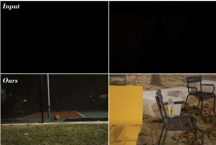
Fig. 6: Input Sony-Total-Dark extreme low-light image with the image enhanced by our CIDNet.
图 6: 输入Sony-Total-Dark极低光图像及经CIDNet增强后的效果。
LOL. The LOL dataset has v1 [6] and v2 [27] versions. LOL-v2 is divided into real and synthetic subsets. The training and testing sets are split in proportion to 485:15, 689:100, and 900:100 on LOL-v1, LOL-v2-Real, and LOL-v2-Synthetic. For LOLv1 and LOLv2-Real, we crop the training images into $400\times400$ patches and train CIDNet for 1500 epochs with a batch size of 8. For LOLv2-Synthetic, we set the batch size to 1 and trained 500 epochs without cropping.
LOL。LOL数据集包含v1 [6]和v2 [27]两个版本。LOL-v2分为真实和合成两个子集。训练集与测试集在LOL-v1、LOL-v2-Real和LOL-v2-Synthetic上的划分比例分别为485:15、689:100和900:100。对于LOLv1和LOLv2-Real,我们将训练图像裁剪为$400\times400$的块,以批量大小8训练CIDNet 1500轮次。对于LOLv2-Synthetic,我们设置批量大小为1,不进行裁剪并训练500轮次。
SICE. The original SICE dataset [32] contains a total of 589 sets of low-light and overexposed images, and the training set, validation set, and test set are divided into three groups according to 7:1:2. We train on the SICE training set with the batch size of 10 and test on the datasets SICE-Mix and SICEGrad [33]. We crop the original SICE image by $160\times160$ and train CIDNet over 1000 epochs.
SICE。原始SICE数据集[32]共包含589组低光和过曝图像,训练集、验证集和测试集按7:1:2的比例划分。我们在SICE训练集上以批次大小(batch size)为10进行训练,并在SICE-Mix和SICEGrad[33]数据集上测试。将原始SICE图像裁剪为$160\times160$尺寸,并对CIDNet进行1000轮(epoch)训练。
Sony-Total-Dark. This dataset is a customized version of the subset of SID dataset captured by the Sony $\alpha7\mathrm{{S}}$ II camera, which is adopted for evaluation. There are 2697 shortlong-exposure RAW image pairs. To make this dataset more challenging, we convert the RAW format images to sRGB images with no gamma correction as Fig. 6, which resulted in images becoming extremely dark. We crop the training images into $256\times256$ patches and train CIDNet for 1500 epochs with a batch size of 4.
Sony-Total-Dark。该数据集是SID数据集中由Sony $\alpha7\mathrm{{S}}$ II相机拍摄的子集定制版本,用于评估。包含2697组短长曝光RAW图像对。为提升挑战性,我们将RAW格式图像转换为未经伽马校正的sRGB图像(如图6所示),导致图像变得极暗。训练图像被裁剪为$256\times256$的块,以批量大小4训练CIDNet 1500轮次。
TABLE II: Quantitative comparisons $\mathrm{LPIPS/FLOPs\downarrow}$ on LOL (v1 and v2) datasets. GT Mean represents the gamma-corrected image by Ground Truth. The best result is in red color.
表 II: 定量比较 $\mathrm{LPIPS/FLOPs\downarrow}$ 在 LOL (v1 和 v2) 数据集上的表现。GT Mean 表示 Ground Truth 的伽马校正图像。最佳结果以红色标注。
| 方法 | LOLv1 | LOLv2-Real | LOLv2-Syn | 复杂度 FLOPs/G↓ | |||
|---|---|---|---|---|---|---|---|
| Normal | GT Mean | Normal | GT Mean | Normal | GT Mean | ||
| EnlightenGAN | 0.322 | 0.317 | 0.309 | 0.301 | 0.220 | 0.213 | 61.01 |
| RetinexNet | 0.474 | 0.470 | 0.543 | 0.519 | 0.255 | 0.247 | 587.47 |
| LLFormer | 0.175 | 0.167 | 0.211 | 0.209 | 0.066 | 0.061 | 22.52 |
| LLFlow | 0.119 | 0.117 | 0.176 | 0.158 | 0.067 | 0.063 | 358.4 |
| LEDNet | 0.118 | 0.113 | 0.120 | 0.114 | 0.061 | 0.056 | 35.92 |
| RetinexFormer | 0.131 | 0.129 | 0.171 | 0.166 | 0.059 | 0.056 | 15.85 |
| CIDNet | 0.086 | 0.079 | 0.108 | 0.101 | 0.045 | 0.040 | 7.57 |
LOL-Blur. The dataset, LOL-Blur [35], contains 12,000 low-blur/normal-sharp pairs with diverse darkness and blurs in 200 different scenarios. The training and testing sets are split in proportion to 17:3. In our experiment, we use low-blur and high-sharp-scaled sets for training and testing. We crop the training images into $256\times256$ patches and train CIDNet for 300 epochs with a batch size of 8. Unlike other experiments, here we use ${l}{m s e}$ Loss instead of $l_{1}$ Loss in Eq. 12.
LOL-Blur。该数据集LOL-Blur [35]包含12,000对低模糊/正常清晰度的图像,涵盖200种不同场景下的多样化暗度和模糊程度。训练集与测试集按17:3比例划分。实验中,我们采用低模糊和高清晰度缩放集进行训练与测试。将训练图像裁剪为$256\times256$的块,以批量大小8训练CIDNet 300个周期。与其他实验不同,此处使用${l}{m s e}$损失函数替代公式12中的$l_{1}$损失。
Experiment Settings. We implement our CIDNet by PyTorch. The model is trained with the Adam [42] optimizer $\textstyle\beta_{1}=0.9$ and $\beta_{2}=0.999)$ for at least 300 epochs by using a single NIVIDA 2080Ti or 3090 GPU. The learning rate is initially set to $1\times10^{-4}$ and then steadily decreased to $1\times10^{-7}$ by the cosine annealing scheme [43] during the training process. In testing stage, we pad the input images to be a multiplier of $8\times8$ using reflect padding on both sides. After inference, we crop the padded image back to its original size. Since the outliers are existed in the outputs of UNets, we simply use clip operation to HVI space, which follows , $0\leq i\leq1}$ , where $\boldsymbol{p}=(h,v,i)$ is the three-dimensional coordinates in HVI color space, and $k$ denotes the density $k$ in Eq. 2.
实验设置。我们使用PyTorch实现CIDNet。模型采用Adam [42]优化器进行训练,参数设置为$\textstyle\beta_{1}=0.9$和$\beta_{2}=0.999)$,在单张NVIDIA 2080Ti或3090 GPU上至少训练300轮。初始学习率设为$1\times10^{-4}$,随后通过余弦退火策略[43]在训练过程中逐步降至$1\times10^{-7}$。测试阶段,我们对输入图像进行反射填充,使其尺寸变为$8\times8$的整数倍。推理完成后,将填充部分裁剪恢复至原始尺寸。由于UNet输出存在异常值,我们直接在HVI色彩空间进行截断操作,约束条件为,$0\leq i\leq1}$。其中$\boldsymbol{p}=(h,v,i)$表示HVI色彩空间的三维坐标,$k$对应公式2中的密度参数$k$。
Evaluation Metrics. For the paired dataset, we adopt the
评估指标。对于配对数据集,我们采用

Fig. 7: Five unpaired datasets are compared visually, and we randomly select one image in each dataset to compare with the other methods. Our CIDNet enhances dark details and illumination to a suitable interval, which is better than the other methods.
图 7: 对五个非配对数据集进行可视化对比,我们随机选取各数据集中的一张图像与其他方法进行比较。我们的CIDNet将暗部细节和光照增强至适宜区间,效果优于其他方法。
TABLE III: Quantitative comparison on five unpaired datasets with $\mathbf{BRISQUE}{\downarrow}$ and $\mathbf{NIQE}\downarrow$ . The best result is in red color.
表 III: 在五个无配对数据集上使用 $\mathbf{BRISQUE}{\downarrow}$ 和 $\mathbf{NIQE}\downarrow$ 的定量比较。最佳结果以红色标注。
| 方法 | DICM_BRISQUE↓ | DICM_NIQE↓ | LIME_BRISQUE↓ | LIME_NIQE↓ | MEF_BRISQUE↓ | MEF_NIQE↓ | NPE_BRISQUE↓ | NPE_NIQE↓ | VV_BRISQUE↓ | VV_NIQE↓ |
|---|---|---|---|---|---|---|---|---|---|---|
| KinD [2] | 48.72 | 5.15 | 39.91 | 5.03 | 49.94 | 5.47 | 36.85 | 4.98 | 50.56 | 4.30 |
| ZeroDCE [4] | 27.56 | 4.58 | 20.44 | 5.82 | 17.32 | 4.93 | 20.72 | 4.53 | 34.66 | 4.81 |
| RUAS [39] | 38.75 | 5.21 | 27.59 | 4.26 | 23.68 | 3.83 | 47.85 | 5.53 | 38.37 | 4.29 |
| LLFlow [5] | 26.36 | 4.06 | 27.06 | 4.59 | 30.27 | 4.70 | 28.86 | 4.67 | 31.67 | 4.04 |
| SNR-Aware [15] | 37.35 | 4.71 | 39.22 | 5.74 | 31.28 | 4.18 | 26.65 | 4.32 | 78.72 | 9.87 |
| PairLIE [7] | 33.31 | 4.03 | 25.23 | 4.58 | 27.53 | 4.06 | 28.27 | 4.18 | 39.13 | 3.57 |
| CIDNet | 21.47 | 3.79 | 16.25 | 4.13 | 13.77 | 3.56 | 18.92 | 3.74 | 30.63 | 3.21 |
Peak Signal-to-Noise Ratio (PSNR) and Structural Similarity (SSIM) [44] as the distortion metrics. To comprehensively evaluate the perceptual quality of restored images, we report Learned Perceptual Image Patch Similarity (LPIPS) [45] by using AlexNet [46] for references as a perceptual metric. For the unpaired datasets, we evaluated single recovered images using BRISQUE [47] and NIQE [48] perceptual ly.
峰值信噪比 (PSNR) 和结构相似性 (SSIM) [44] 作为失真度量指标。为全面评估修复图像的感知质量,我们采用基于 AlexNet [46] 的 Learned Perceptual Image Patch Similarity (LPIPS) [45] 作为感知指标。针对非配对数据集,我们使用 BRISQUE [47] 和 NIQE [48] 对单幅复原图像进行感知质量评估。
B. Evaluation on Image Enhancement
B. 图像增强评估
LOL Datasets Results. We quantitatively compare our CIDNet with many SOTA methods as shown in Table I and II. It can be found that our method is optimal on almost all metrics for both LOLv1 and LOLv2 datasets. Comparing the two tables comprehensively, it can be seen that CIDNet achieves six new SOTA SSIM and LPIPS results on three subsets of LOL (v1 and v2) dataset with only 7.57 GFLOPs. It outperforms the current SOTA method Ret in ex former in terms of both PSNR and SSIM under GT Mean while LPIPS improves by $38%$ , $39%$ , and $29%$ , respectively, and FLOPs decreased by $52%$ . Compared to 3DLUT with about the same size of FLOPs, our method significantly improves the PSNR by 6.791, 7.944, and 7.393 dB. It may be observed in Figure 5 that our model restores colors extremely well, which may be attributed to the HVI color space.
LOL数据集结果。我们在表I和表II中对CIDNet与多种SOTA方法进行了定量比较。可以发现,我们的方法在LOLv1和LOLv2数据集上几乎所有指标都达到最优。综合对比两表可知,CIDNet仅以7.57 GFLOPs的计算量,在LOL (v1和v2) 数据集的三个子集上创造了六项SSIM与LPIPS的新SOTA记录。在GT Mean标准下,其PSNR和SSIM均优于当前SOTA方法Retinexformer,LPIPS指标分别提升38%、39%和29%,FLOPs降低52%。与计算量相近的3DLUT相比,我们的方法将PSNR显著提高了6.791、7.944和7.393 dB。如图5所示,我们的模型在色彩还原方面表现优异,这可能归功于HVI色彩空间的应用。
TABLE IV: Quantitative comparison on three hard datasets (SICEMix/Grad and Sony-Total-Dark) with $\mathbf{PSNR}\uparrow$ , $\mathbf{SSIM}\uparrow$ and $\mathbf{LPIPS}\downarrow$ .
表 IV: 在三个困难数据集 (SICEMix/Grad 和 Sony-Total-Dark) 上的定量比较,指标为 $\mathbf{PSNR}\uparrow$、$\mathbf{SSIM}\uparrow$ 和 $\mathbf{LPIPS}\downarrow$。
| 方法 | SICE-Mix PSNR↑ | SSIM↑ | LPIPS↓ | SICE-Grad PSNR↑ | SSIM↑ | LPIPS↓ | Sony-Total-Dark PSNR↑ | SSIM↑ | LPIPS↓ |
|---|---|---|---|---|---|---|---|---|---|
| RetinexNet | 12.397 | 0.606 | 0.407 | 12.450 | 0.619 | 0.364 | 15.695 | 0.395 | 0.743 |
| ZeroDCE | 12.428 | 0.633 | 0.382 | 12.475 | 0.644 | 0.334 | 14.087 | 0.090 | 0.813 |
| URetinexNet | 10.903 | 0.600 | 0.402 | 10.894 | 0.610 | 0.356 | 15.519 | 0.323 | 0.599 |
| RUAS | 8.684 | 0.493 | 0.525 | 8.628 | 0.494 | 0.499 | 12.622 | 0.081 | 0.920 |
| LLFlow | 12.737 | 0.617 | 0.388 | 12.737 | 0.617 | 0.388 | 16.226 | 0.367 | 0.619 |
| LEDNet | 12.668 | 0.579 | 0.412 | 12.551 | 0.576 | 0.383 | 20.830 | 0.648 | 0.471 |
| CIDNet | 13.425 | 0.636 | 0.362 | 13.446 | 0.648 | 0.318 | 22.904 | 0.676 | 0.411 |
SICE and Sony-total-Dark. To verify that our model also performs well on large-scale datasets, we conducted experiments on two extremely difficult-to-recover datasets, SICE (including Mix and Grad) and SID-Total-Dark. The three metrics of our CIDNet are optimal on all three test sets as Table IV. especially on the Sony-Total-Dark dataset, which outperforms LEDNet by $9.96%$ for the PSNR, $4.32%$ for the SSIM, $12.74%$ for the LPIPS metrics.
SICE与Sony-total-Dark。为验证我们的模型在大规模数据集上同样表现优异,我们在两个极难恢复的数据集SICE(包含Mix和Grad)和SID-Total-Dark上进行了实验。如表IV所示,我们的CIDNet在全部三个测试集上的三项指标均达到最优,尤其在Sony-Total-Dark数据集上,PSNR指标超越LEDNet达$9.96%$,SSIM指标提升$4.32%$,LPIPS指标改善$12.74%$。
Unpaired Datasets Experiments. In the case of unpaired datasets DICM, LIME, MEF, NPE, and VV, where Ground Truth is unavailable, we evaluate the effectiveness of models trained on LOLv1 or LOLv2-Syn using various methods, and measure their performance using BRISQUE and NIQE metrics. We report our comparisons against SOTA methods as Table III, where our method outperformed all
非配对数据集实验。对于没有真实值 (Ground Truth) 的DICM、LIME、MEF、NPE和VV等非配对数据集,我们评估了基于LOLv1或LOLv2-Syn训练模型的效果,并使用BRISQUE和NIQE指标衡量其性能。如表 III 所示,我们的方法优于所有SOTA方法。
TABLE V: Ablation of CIDNet module designs. The first row is a simple UNet baseline [49] without attention module. The row (2), (3), (4), (6), and (7) (where the rows with LCA but without CrossAttn) use Self-Attention [40] to replace Cross-Attention.
表 V: CIDNet模块设计的消融实验。第一行是不带注意力模块的简单UNet基线[49]。第(2)、(3)、(4)、(6)和(7)行(使用LCA但不使用CrossAttn的行)用Self-Attention[40]替代了Cross-Attention。
| ColorSpace | LCA | Dual-branch | CrossAttn | PSNR↑ | SSIM↑ | |
|---|---|---|---|---|---|---|
| 1 | sRGB | 16.518 | 0.721 | |||
| 2 | sRGB | √ | 18.606 | 0.822 | ||
| 3 | HSV | √ | 13.237 | 0.365 | ||
| 4 | HSV | √ | √ | 10.236 | 0.254 | |
| 5 | HSV | √ | √ | √ | 13.668 | 0.407 |
| 6 | HVI | √ | 22.000 | 0.853 | ||
| 7 | HVI | √ | √ | 23.159 | 0.854 | |
| 8 | HVI | √ | √ | √ | 24.111 | 0.868 |

Fig. 8: The visual quality comparison results on LOLv2-Real dataset with various LCA blocks (by removing submodules in the LCA). (e) Full LCA denotes the original design of the LCA block.
图 8: 在LOLv2-Real数据集上采用不同LCA模块(通过移除LCA中的子模块)的视觉质量对比结果。(e) Full LCA表示LCA模块的原始设计。

Fig. 9: Ablation experiment of the submodules CAB, IEL, and CDL in LCA. The impact of CAB is significantly higher than the other two modules, indicating that our designed cross-attention can better enhance the image to the appropriate brightness level. (Full LCA denotes the origin design of the LCA block.)
图 9: LCA中CAB、IEL和CDL子模块的消融实验。CAB的影响显著高于其他两个模块,表明我们设计的交叉注意力能更好地将图像增强到合适的亮度水平。(Full LCA表示LCA模块的原始设计。)
previous SOTA methods. Notably, our method exhibits a substantial improvement in the NIQE metric compared to other approaches.
先前的最先进方法。值得注意的是,与其他方法相比,我们的方法在NIQE指标上表现出显著提升。
For each of these five unpaired datasets, we randomly selected an image in each dataset and compared it visually. As Fig. 7, CIDNet improves the brightness and increases the perceived level of the image while ensuring reasonable color accuracy compared with RUAS, ZeroDCE, RetinexNet, KinD and PairLIE.
在这五个非配对数据集中,我们随机选取了每个数据集中的一张图像进行视觉对比。如图7所示,与RUAS、ZeroDCE、RetinexNet、KinD和PairLIE相比,CIDNet在保证合理色彩准确度的同时提升了图像亮度及视觉感知水平。
C. Ablation Study
C. 消融研究
We conduct extensive ablation studies to validate our HVI color space and several modules. The evaluations are all performed on the LOLv2-Real dataset for fast convergence and stable performance.
我们进行了大量消融实验以验证HVI色彩空间及多个模块的有效性。所有评估均在LOLv2-Real数据集上进行,以确保快速收敛和稳定性能。
Color Spaces. We conduct an ablation on sRGB, HSV and our HVI on CIDNet as Table V. The ranking of image restoration quality with CIDNet is as follows: HVI, sRGB, and HSV. Comparing row (2), (3), and (6), the best is HVI color space, which exists a significant performance enhancement.
色彩空间。我们在CIDNet上对sRGB、HSV和我们的HVI进行了消融实验,如表V所示。使用CIDNet进行图像恢复的质量排名如下:HVI、sRGB和HSV。比较行(2)、(3)和(6),最佳的是HVI色彩空间,其性能有显著提升。
Structures and Modules. First, we examine our LCA module in the present color spaces. As shown in Table V row (1), (2), and (6), LCA with baseline gains 2.088, 5.428 dB on PSNR for sRGB and HVI respectively. Second, in our experimental investigation, we have observed distinct statistical patterns between the I-branch and HV-branch. As shown in Table V row (6) and (7), dividing the Enhancement Network into dual branches enhances 1.159 dB in PSNR. Third, by decoupling the image through HVI, a certain correlation between the values of the I-map and the noise of the HVmap can be discovered. To establish the relationship mapping, we incorporate Cross-Attention into the internal of LCA. As Table V row (8), PSNR and SSIM are both greater than row (7) by 0.952 dB and 0.014. Last, as Fig. 9, removing the CAB, CDL or IEL clearly shows a decrease effect of PSNR and SSIM, which demonstrates the effectiveness of sub-modules in LCA block. The visual quality comparisons are shown in Fig. 8. Specifically, removing CAB leads to unstable brightness enhancement, resulting in local overexposure and artifacts. On the other hand, removing IEL or CDL results in excessively dark brightness, thereby affecting the details.
结构与模块。首先,我们在现有色彩空间中检验LCA模块。如表V第(1)、(2)和(6)行所示,带基线的LCA在sRGB和HVI色彩空间上分别获得2.088dB和5.428dB的PSNR提升。其次,实验研究发现I分支与HV分支存在明显统计差异。如表V第(6)和(7)行所示,将增强网络拆分为双分支可使PSNR提升1.159dB。第三,通过HVI解耦图像后,可发现I-map数值与HVmap噪声间存在特定关联。为建立关系映射,我们在LCA内部引入交叉注意力机制。如表V第(8)行所示,其PSNR和SSIM分别比第(7)行提高0.952dB和0.014。最后如图9所示,移除CAB、CDL或IEL会明显降低PSNR和SSIM效果,这证明了LCA块中各子模块的有效性。视觉质量对比结果如图8所示:移除CAB会导致亮度增强不稳定,产生局部过曝和伪影;而移除IEL或CDL则会造成亮度过暗,进而影响细节表现。

Fig. 10: Ablation of losses in our HVI color space, the sRGB color space, and the potential feature space as the perceptual (Perc.) loss with VGG19 network [36]. In the group (4), we incorporate the perceptual loss into both the HVI and sRGB color spaces simultaneously.
图 10: 在HVI色彩空间、sRGB色彩空间以及作为感知损失(Perc. loss)的VGG19网络[36]潜在特征空间中进行的损失消融实验。在第(4)组中,我们同时在HVI和sRGB色彩空间中引入了感知损失。
Ablation on loss function. We conduct an ablation by progressively adding loss on (1)HVI-map, (2)sRGB-image, (3)HVI and sRGB, (4)Perceptual loss on both color space as Table 10. Compared to the previous groups, the results of including the loss in all spaces in group (4) shows an improvement in PSNR of 1.998 dB, 1.792 dB, and 0.684 dB. This demonstrates the effectiveness of the loss function we designed.
损失函数消融实验。我们通过逐步增加损失函数进行消融实验:(1) HVI-map、(2) sRGB-image、(3) HVI和sRGB、(4) 如表10所示的双色彩空间感知损失。与之前组别相比,第(4)组在所有色彩空间加入损失函数的结果显示PSNR提升了1.998 dB、1.792 dB和0.684 dB,这证明了我们设计的损失函数的有效性。
Analysis. Above experiments sequentially verify the superiority of our the HVI color space, the LCA block, and the dual-branch Enhancement Network with Cross-Attention. For loss ablation experiment, the HVI color space needs to be supervised by the sRGB space losses in order to perform.
分析。上述实验依次验证了HVI色彩空间、LCA模块和带交叉注意力的双分支增强网络(HVI color space, LCA block, dual-branch Enhancement Network with Cross-Attention)的优越性。在损失函数消融实验中,HVI色彩空间需要通过sRGB空间损失(sRGB space losses)进行监督才能有效工作。

Fig. 11: Comparison of loss function computation positions. The trainable parameter $k$ is highlighted within the red box. (Zoom in for the best view.)
图 11: 损失函数计算位置对比。可训练参数 $k$ 在红色框内高亮显示。(放大查看最佳效果)
Loss Discussion: Why is HVI loss performance weaker than RGB loss? In Table 10, the results in group (2) outperform those in the first group. The reason is that the loss functions of HVI and RGB operate at different positions in our network. As presented in Fig. 11, in between the losses of HVI and RGB lies the inverse transformation of HVI, which incorporates a trainable parameter $k$ . Using only the HVI loss does not allow $k$ to converge to the optimal solution and the loss in RGB color space is needed to assist in the training process. Therefore, the combination of HVI and RGB losses has achieved better performance as shown in the third group of Fig. 10.
损失讨论:为何HVI损失性能弱于RGB损失?
在表10中,第二组结果优于第一组。这是因为HVI与RGB的损失函数在网络中的不同位置起作用。如图11所示,HVI与RGB损失之间存在着包含可训练参数 $k$ 的HVI逆变换。仅使用HVI损失无法使 $k$ 收敛到最优解,需要RGB色彩空间的损失辅助训练过程。因此,如图10第三组所示,结合HVI与RGB损失能获得更优性能。
D. Robustness Experiments
D. 鲁棒性实验
LOL-Blur. Long exposures in dimly lit environments can result in photos that are prone to blurring. To verify the robustness ability of our model, we conduct experiments on the low-light blur dataset LOL-Blur.
LOL-Blur。在光线昏暗的环境中进行长时间曝光可能导致照片容易模糊。为了验证我们模型的鲁棒性,我们在低光照模糊数据集LOL-Blur上进行了实验。
TABLE VI: Quantitative evaluation on LOL-Blur dataset. $\mathrm{PSNR}\uparrow$ and $\mathrm{SSIM\uparrow}$ : the higher, the better; $\mathrm{LPIPS}\downarrow$ and $\mathrm{FLOPs\downarrow}$ : the lower, the better. The symbol $\because$ indicates that we use DeblurGAN-v2 trained on RealBlur [50] dataset. $\ddagger^{,}$ indicates the network is retrained on the LOL-Blur dataset. The highest result is in red color.
表 VI: LOL-Blur 数据集定量评估。$\mathrm{PSNR}\uparrow$ 和 $\mathrm{SSIM\uparrow}$ : 数值越高越好;$\mathrm{LPIPS}\downarrow$ 和 $\mathrm{FLOPs\downarrow}$ : 数值越低越好。符号 $\because$ 表示我们使用了在 RealBlur [50] 数据集上训练的 DeblurGAN-v2。$\ddagger^{,}$ 表示网络在 LOL-Blur 数据集上进行了重新训练。最高结果以红色标注。
| 方法 | PSNR↑ | SSIM↑ | LPIPS↓ | FLOPs↓ |
|---|---|---|---|---|
| ZeroDCE[4]→MIMO[51] | 17.680 | 0.542 | 0.422 | |
| DeblurGANf[52]→ZeroDCE[4] | 18.330 | 0.589 | 0.384 | - |
| RetinexFormer [14] | 22.904 | 0.824 | 0.236 | 15.85 |
| MIMO[51] | 24.410 | 0.835 | 0.183 | 62.36 |
| LEDNet [35] | 25.271 | 0.859 | 0.141 | 35.93 |
| CIDNet | 26.572 | 0.890 | 0.120 | 7.57 |
TABLE VII: Robustness testing experiments. All methods is trained on the LOLv1 and tested in the LOLv2-Syn dataset. The best result is in red color.
表 VII: 鲁棒性测试实验。所有方法均在 LOLv1 上训练,并在 LOLv2-Syn 数据集中测试。最佳结果以红色标注。
| 方法 | LLFlow | RUAS | PairLIE | RetinexFormer | LEDNet | CIDNet |
|---|---|---|---|---|---|---|
| PSNR↑ | 17.1191 | 15.3257 | 19.0743 | 16.1834 | 16.6210 | 18.6382 |
| SSIM↑ | 0.8117 | 0.4883 | 0.7965 | 0.7693 | 0.7733 | 0.8200 |
| LPIPS↓ | 0.2239 | 0.4577 | 0.2300 | 0.2515 | 0.2196 | 0.2154 |

Fig. 12: Visual comparison on LOL-Blur dataset. Compared to other methods, our CIDNet is closer to Ground Truth and more dominant in visual recognition. (Zoom in for best view.)
图 12: LOL-Blur 数据集上的视觉对比。与其他方法相比,我们的 CIDNet 更接近真实值 (Ground Truth) ,在视觉识别方面更具优势。(建议放大查看最佳效果。)
In the first set, we perform lighting-up with ZeroDCE and then deblurring with MIMO [51]. In the second set, we perform deblurring with DeblurGAN-v2 [52] and then light up with ZeroDCE. In the third group, we have retrained on LOLBlur with four methods, Ret in ex Former, MIMO, and LEDNet, and compared them with our CIDNet. The results (as Table VI) show that the quantitative comparison of CIDNet against the current stage SOTA method LEDNet by $5.15%$ , $3.61%$ , and $14.89%$ in PSNR, SSIM, and LPIPS metrics respectively. Not only that, the FLOPs of our model are the lowest among these methods.
在第一组实验中,我们先用ZeroDCE进行光照增强,再用MIMO[51]进行去模糊处理。第二组实验则先用DeblurGAN-v2[52]去模糊,再用ZeroDCE提亮。第三组实验我们在LOLBlur数据集上重新训练了四种方法(RetinexFormer、MIMO和LEDNet),并与我们的CIDNet进行对比。结果(如表VI所示)表明,CIDNet在PSNR、SSIM和LPIPS指标上分别比当前最优方法LEDNet提升了5.15%、3.61%和14.89%。不仅如此,我们模型的FLOPs在这些方法中也是最低的。
As shown in Fig. 12, we have taken a set of blurred images, recovered them using different methods, and compared them with Ground Truth. The experimental results reveal that the image reconstructions achieved by CIDNet exhibit a notable improvement in visual comfort and perceptual recognition, thereby enhancing the overall quality and interpret ability of the generated images.
如图 12 所示,我们采集了一组模糊图像,分别采用不同方法进行复原并与真实值 (Ground Truth) 对比。实验结果表明,CIDNet 实现的图像重建在视觉舒适度与感知辨识度方面均有显著提升,从而全面增强了生成图像的质量与可解释性。
Cross dataset validation. To verify the generalization ability of our model, we take the model trained on LOLv1 [6] and tested it on LOLv2-Syn [27] as Table VII. Compared with three supervised learning SOTA models, LLFlow [5], Ret in ex Former [14], and LEDNet [35], our model comprehensively outperforms in three metrics. And compared with the unsupervised models PairLIE [7] and RUAS [39], which have better generalization ability, our CIDNet also completely outperforms SSIM and LPIPS.
跨数据集验证。为验证我们模型的泛化能力,我们采用在LOLv1 [6]上训练的模型并在LOLv2-Syn [27]上进行测试,如表VII所示。与三种监督学习SOTA模型LLFlow [5]、RetinexFormer [14]和LEDNet [35]相比,我们的模型在三个指标上全面胜出。相较于具有更好泛化能力的无监督模型PairLIE [7]和RUAS [39],我们的CIDNet在SSIM和LPIPS指标上也完全超越。
The effect of HVIT in other methods. We employ the HVI transform as a versatile module to examine the resilience of our HVI space across multiple models. To this end, the HVIT and PHVIT are incorporated into four supervised models, Ret in ex Former, LEDNet, Restormer, and SNR-Aware. Subsequently, these models are retrained and evaluated on the LOLv2-Real [27] dataset. The outcomes, as illustrated in Table VIII, demonstrate the remarkable enhancement achieved by our HVI space in the performance of each method. Impressively, all eleven metrics associated with the four methods exhibit substantial improvements. Moreover, the proposed CIDNet demonstrates superior performance not only in terms of PSNR and SSIM, but also exhibits the shortest CPU (AMD Ryzen 9 5900HX) and GPU (NVIDIA 2080Ti) inference time and minimal computational (FLOPs) overhead.
HVIT在其他方法中的效果。我们将HVI变换作为一个多功能模块,用于检验HVI空间在多种模型中的鲁棒性。为此,HVIT和PHVIT被集成到四种监督模型中:RetinexFormer、LEDNet、Restormer和SNR-Aware。随后,这些模型在LOLv2-Real [27]数据集上进行了重新训练和评估。结果如表VIII所示,证明了我们的HVI空间对每种方法性能的显著提升。令人印象深刻的是,与这四种方法相关的所有十一个指标都显示出实质性改进。此外,所提出的CIDNet不仅在PSNR和SSIM方面表现出优越性能,还展现出最短的CPU (AMD Ryzen 9 5900HX)和GPU (NVIDIA 2080Ti)推理时间以及最小的计算量 (FLOPs)开销。
TABLE VIII: HVI transform robustness validation experiments. Embedding HVI transform into other methods and training/testing on LOLv2-Real. Value in brackets represents the amount of better numerical changes with red color. The best result of PSNR/SSIM and $\mathrm{LPIPS/FLOPs\downarrow}$ is in bolded. The lowest time of inference with $256\times256$ in three channels is also in bolded.
表 VIII: HVI变换鲁棒性验证实验。将HVI变换嵌入其他方法并在LOLv2-Real数据集上训练/测试。括号内数值标红表示正向提升幅度。PSNR/SSIM和$\mathrm{LPIPS/FLOPs\downarrow}$最优结果以粗体标注。$256\times256$三通道推理时间最短值同样加粗显示。
| 方法 | RetinexFormer | LEDNet | Restormer | SNR-Aware | CIDNet |
|---|---|---|---|---|---|
| PSNR↑ | 23.600(+0.806) | 23.394(+3.456) | 23.234(+4.541) | 22.251(+0.771) | 24.111 |
| SSIM↑ | 0.865(+0.025) | 0.837(+0.010) | 0.866(+0.032) | 0.840(-0.009) | 0.868 |
| LPIPS↓ | 0.113(-0.058) | 0.117(-0.003) | 0.093(-0.022) | 0.117(-0.040) | 0.108 |
| FLOPs/G↓ | 15.85 | 35.92 | 114.25 | 26.35 | 7.57 |
| GPU耗时/s | 0.062 | 0.070 | 0.183 | 0.054 | 0.053 |
| CPU耗时/s↓ | 0.594 | 0.846 | 5.898 | 1.751 | 0.416 |
TABLE IX: Ablation of three different types of inputs in Enhancement Network. Each distinct convolution layers will extract and generate corresponding intensity features (as I-Feature) and HVfeatures from different input maps (the type of input is indicated in the columns I-Feature and HV-Feature). The best result is in red color.
表 IX: 增强网络中三种不同类型输入的消融实验。各独立卷积层将从不同输入图(输入类型在I-Feature和HV-Feature列中标注)中提取并生成对应的强度特征(I-Feature)和HV特征。最佳结果以红色标注。
| 类型 | I-特征 | HV-特征 | PSNR↑ | SSIM↑ | LPIPS√ |
|---|---|---|---|---|---|
| (1) Half-HVIT | intensity | HVI-Map | 24.111 | 0.868 | 0.108 |
| (2) Separate-HVIT | intensity | HV-Map | 23.734 | 0.857 | 0.141 |
| (3) Full-HVIT | HVI-Map | HVI-Map | 23.814 | 0.859 | 0.127 |
E. Variant HVIT Experiments and Discussion
E. HVIT变体实验与讨论
To investigate how the first two $3\times3$ convolution layers (in Enhancement Network) learned to generate I-feature and HVfeature, we further develop three different HVIT by changing the inputs. As shown in Table IX row (1), the Half-HVIT utilized in our pipeline generates intensity features (here in after abbreviated as I-Features) from the intensity Map and HVFeatures from the HVI-Map. We have respectively modified the input of I-Features and HV-Features, leading to the creation of two new HVIT models in Table IX row (2) and row (3). The Separate-HVIT replaces the input of HV-Feature with HVMap, while the Full-HVIT substitutes the input of I-Feature with HVI-Map.
为了研究前两个$3\times3$卷积层(位于增强网络中)如何学习生成I特征和HV特征,我们通过改变输入进一步开发了三种不同的HVIT变体。如表IX第(1)行所示,本方案采用的Half-HVIT从强度图生成强度特征(以下简称I特征),从HVI图生成HV特征。我们分别修改了I特征和HV特征的输入,从而在表IX第(2)行和第(3)行创建了两个新HVIT模型:Separate-HVIT将HV特征的输入替换为HV图,而Full-HVIT则将I特征的输入替换为HVI图。
As a result, the Half-HVIT achieves the best restoration results among the three HVIT models. The performance drop of the Separate-HVIT is more pronounced, with reductions of 0.377 dB in PSNR, 0.011 in SSIM, and 0.033 in LPIPS. This can be attributed to the lower information content in the HV features compared to the HVI-Map, which lacks guidance from the intensity part. On the other hand, the performance decline of the Full-HVIT was due to the interference noise information in the HVI-Map for extracting I-Features, leading to convolutional layers failing to accurately extract key features.
因此,Half-HVIT在三种HVIT模型中取得了最佳修复效果。Separate-HVIT的性能下降更为明显,PSNR降低了0.377 dB,SSIM降低了0.011,LPIPS降低了0.033。这归因于HV特征的信息量低于HVI-Map,且缺乏强度部分的引导。另一方面,Full-HVIT的性能下降是由于HVI-Map中的干扰噪声信息影响了I-Features的提取,导致卷积层无法准确提取关键特征。
VI. CONCLUSION
VI. 结论
In this paper, we present a novel method for low-light image enhancement using the proposed HVI color space with trainable parameters and the CIDNet to decouple image brightness and color and adapt to various illumination scales. The dual-branch network, build upon the HVI color space, simultaneously processes brightness and color, aided by the plug-and-play LCA module and symmetric HVI Transform module. Our CIDNet outperforms all types of SOTA methods across 11 datasets with lower FLOPs and parameters.
本文提出了一种基于新型HVI色彩空间与可训练参数的弱光图像增强方法,通过CIDNet实现图像亮度与色彩的分离处理,并自适应不同光照尺度。该双分支网络依托HVI色彩空间架构,结合即插即用LCA模块和对称HVI转换模块,同步处理亮度与色彩信息。实验表明,CIDNet在11个数据集上以更低计算量(FLOPs)和参数量全面超越各类SOTA方法。