Neural Pre-Processing: A Learning Framework for End-to-end Brain MRI Pre-processing

Neural Pre-Processing: 端到端脑部MRI预处理的学xi框架

Abstract. Head MRI pre-processing involves converting raw images to an intensity-normalized, skull-stripped brain in a standard coordinate space. In this paper, we propose an end-to-end weakly supervised learning approach, called Neural Pre-processing (NPP), for solving all three sub-tasks simultaneously via a neural network, trained on a large dataset without individual sub-task supervision. Because the overall objective is highly under-constrained, we explicitly disentangle geometricpreserving intensity mapping (skull-stripping and intensity normalization) and spatial transformation (spatial normalization). Quantitative results show that our model outperforms state-of-the-art methods which tackle only a single sub-task. Our ablation experiments demonstrate the importance of the architecture design we chose for NPP. Furthermore, NPP affords the user the flexibility to control each of these tasks at inference time. The code and model are freely-available at https: //github.com/Novestars/Neural-Pre-processing.

摘要：头部MRI预处理涉及将原始图像转换为标准坐标空间中强度归一化且去除颅骨的脑部图像。本文提出一种端到端弱监督学习方法——神经预处理(NPP)，通过在大规模数据集上训练的神经网络同时解决这三个子任务，且无需单独的子任务监督。由于整体目标高度欠约束，我们显式解耦了保持几何特性的强度映射(去颅骨和强度归一化)与空间变换(空间归一化)。定量结果表明，该模型在仅处理单个子任务的先进方法中表现更优。消融实验验证了我们为NPP设计的架构重要性。此外，NPP在推理时允许用户灵活控制每个子任务。代码与模型已在https://github.com/Novestars/Neural-Pre-processing开源。

Keywords: Neural network $^{-1}$ Pre-processing · Brain MRI.

关键词：神经网络 $^{-1}$ · 预处理 · 脑部MRI

1 Introduction

1 引言

Brain magnetic resonance imaging (MRI) is widely-used in clinical practice and neuroscience. Many popular toolkits for pre-processing brain MRI scans exist, e.g., FreeSurfer [9], FSL [25], AFNI [5], and ANTs [3]. These toolkits divide up the pre-processing pipeline into sub-tasks, such as skull-stripping, intensity normalization, and spatial normalization/registration, which often rely on computationally-intensive optimization algorithms.

脑磁共振成像 (MRI) 在临床实践和神经科学领域应用广泛。目前已有许多流行的脑 MRI 扫描预处理工具包，例如 FreeSurfer [9]、FSL [25]、AFNI [5] 和 ANTs [3]。这些工具包将预处理流程划分为多个子任务，例如颅骨剥离、强度归一化和空间归一化/配准，这些任务通常依赖于计算密集型的优化算法。

Recent works have turned to machine learning-based methods to improve preprocessing efficiency. These methods, however, are designed to solve individual sub-tasks, such as SynthStrip [15] for skull-stripping and Voxelmorph [4] for registration. Learning-based methods have advantages in terms of inference time and performance. However, solving sub-tasks independently and serially has the drawback that each step’s performance depends on the previous step. In this paper, we propose a neural network-based approach, which we term Neural PreProcessing (NPP), to solve three basic tasks of pre-processing simultaneously.

最近的研究转向基于机器学习的方法以提高预处理效率。然而这些方法仅针对单个子任务设计，例如用于颅骨剥离的SynthStrip [15] 和用于配准的Voxelmorph [4]。基于学习的方法在推理时间和性能方面具有优势，但独立且串行解决子任务会带来每个步骤的性能依赖于前序步骤的缺陷。本文提出一种基于神经网络的方法（我们称为神经预处理(NPP)），可同步解决预处理中的三项基础任务。

NPP first translates a head MRI scan into a skull-stripped and intensitynormalized brain using a translation module, and then spatially transforms to the standard coordinate space with a spatial transform module. As we demonstrate in our experiments, the design of the architecture is critical for solving these tasks together. Furthermore, NPP offers the flexibility to turn on/off different pre-processing steps at inference time. Our experiments demonstrate that NPP achieves state-of-the-art accuracy in all the sub-tasks we consider.

NPP首先通过一个翻译模块将头部MRI扫描转换为经过颅骨剥离和强度归一化的大脑图像，随后利用空间变换模块将其转换到标准坐标空间。如实验所示，这种架构设计对协同解决这些任务至关重要。此外，NPP在推理阶段可灵活开启/关闭不同的预处理步骤。实验表明，NPP在我们考察的所有子任务中都达到了最先进的精度水平。

2 Methods

2 方法

2.1 Model

2.1 模型

As shown in Fig. 1, our model contains two modules: a geometry-preserving translation module, and a spatial-transform module.

如图 1 所示，我们的模型包含两个模块：几何保持转换模块和空间变换模块。

Geometry-preserving Translation Module. This module converts a brain MRI scan to a skull-stripped and intensity normalized brain. We implement it using a U-Net style [23] $f_{\theta}$ architecture (see Fig. 1), where $\theta$ denotes the model weights. We operational ize skull stripping and intensity normalization as a pixelwise multiplication of the input image with a scalar multiplier field $\chi$ , which is the output of the U-Net $f_{\theta}$ :

几何保持转换模块。该模块将脑部MRI扫描转换为去颅骨且强度归一化的脑部图像。我们采用U-Net风格[23]的$f_{\theta}$架构实现该模块（见图1），其中$\theta$表示模型权重。我们将去颅骨和强度归一化操作实现为输入图像与标量乘子场$\chi$的逐像素相乘，该乘子场是U-Net $f_{\theta}$的输出：

$$
T_{\theta}(x)=f_{\theta}(x)\otimes x,
$$

$$
T_{\theta}(x)=f_{\theta}(x)\otimes x,
$$

where $\bigotimes$ denotes the element-wise (Hadamard) product.

其中 $\bigotimes$ 表示逐元素 (Hadamard) 乘积。

Such a parameter iz ation allows us to impose constraints on $\chi$ . In this work, we penalize high-frequencies in $\chi$ , via the total variation loss described below. Another advantage of $\chi$ is that it can be computed at a lower resolution to boost both training and inference speed, and then up-sampled to the full resolution grid before being multiplied with the input image. This is possible because the multiplier $\chi$ is spatially smooth. In contrast, if we have $f_{\theta}$ directly compute the output image, doing this at a lower resolution means we will inevitably lose high frequency information. In our experiments, we take advantage of this by having the model output the multiplicative field at a grid size that is $1/2$ of the original input grid size along each dimension.

这样的参数化允许我们对 $\chi$ 施加约束。在本工作中，我们通过下文描述的总变差损失来惩罚 $\chi$ 中的高频成分。$\chi$ 的另一个优势是可以在较低分辨率下计算以提升训练和推理速度，随后在与输入图像相乘前上采样至完整分辨率网格。这种操作之所以可行，是因为乘数 $\chi$ 具有空间平滑性。相比之下，若直接让 $f_{\theta}$ 计算输出图像，在较低分辨率下操作将不可避免地丢失高频信息。实验中，我们利用这一特性，让模型输出的乘性场网格尺寸沿每个维度均为原始输入网格尺寸的 $1/2$。

Spatial Transformation Module. Spatial normalization is implemented as a variant of the Spatial Transformer Network (STN) [17]; in our implementation, the STN outputs the 12 parameters of an affine matrix $\boldsymbol{\phi}{a f f}$ . The STN takes as input the bottleneck features from the image translation network $f_{\theta}$ and feeds it through a multi-layer perceptron (MLP) that projects the features to a 12-dimensional vector encoding the affine transformation matrix. This affine transformation is in turn applied to the output of the image translation module $T_{\boldsymbol{\theta}}(\boldsymbol{x})$ via a differentiable resampling layer [17].

空间变换模块。空间归一化通过空间变换网络 (Spatial Transformer Network, STN) [17] 的变体实现；在我们的实现中，STN 输出仿射矩阵 $\boldsymbol{\phi}{a f f}$ 的 12 个参数。STN 以图像翻译网络 $f_{\theta}$ 的瓶颈特征作为输入，并通过多层感知机 (MLP) 将特征投影为编码仿射变换矩阵的 12 维向量。该仿射变换随后通过可微分重采样层 [17] 作用于图像翻译模块 $T_{\boldsymbol{\theta}}(\boldsymbol{x})$ 的输出。

Fig. 1: (Top) An overview of Neural Pre-processing. (Bottom) The network archie c ture of Neural Pre-processing

图 1: (上) 神经预处理 (Neural Pre-processing) 概览。(下) 神经预处理的网络架构

2.2 Loss Function

2.2 损失函数

The objective to minimize is composed of two terms. The first term is a reconstruction loss $L_{r e c}$ . In this paper, we use SSIM [29] for $L_{r e c}$ . The second term penalizes $T_{\theta}$ from making high-frequency intensity changes to the input image, encapsulating our prior knowledge that skull-stripping and MR bias field correction involve a pixel-wise product with a spatially smooth field. In this work, we use a total variation penalty [22] $L_{T V}$ on the multiplier field $\chi$ , which promotes sparsity of spatial gradients in $\chi$ . The final objective is:

最小化目标由两项组成。第一项是重建损失 $L_{r e c}$。本文使用 SSIM [29] 作为 $L_{r e c}$。第二项惩罚 $T_{\theta}$ 对输入图像进行高频强度变化，体现了我们的先验知识：颅骨剥离和 MR 偏置场校正涉及与空间平滑场的逐像素乘积。本工作采用总变分惩罚 [22] $L_{T V}$ 作用于乘子场 $\chi$，以促进 $\chi$ 中空间梯度的稀疏性。最终目标为：

$$
\underset{\theta}{\arg\operatorname*{min}}L_{r e c}(T_{\theta}(x)\circ\varPhi_{a f f},x_{g t})+\lambda L_{T V}(\chi),
$$

$$
\underset{\theta}{\arg\operatorname*{min}}L_{r e c}(T_{\theta}(x)\circ\varPhi_{a f f},x_{g t})+\lambda L_{T V}(\chi),
$$

where $x_{g t}$ is the pre-processed ground truth images, $\lambda\geq0$ controls the trade-off between the two loss terms, and $\circ$ denotes a spatial transformation.

其中 $x_{g t}$ 是预处理后的真实图像，$\lambda\geq0$ 控制两个损失项之间的权衡，$\circ$ 表示空间变换。

Conditioning on $\lambda$ . Classically, hyper parameters like $\lambda$ are tuned on a held-out validation set - a computationally-intensive task which requires training multiple models corresponding to different values of $\lambda$ . To avoid this, we condition on $\lambda$ in $f_{\theta}$ by passing in $\lambda$ as an input to a separate MLP $h_{\phi}(\lambda)$ (see Fig. 1), which generates a $\lambda$ -conditional scale and bias for each channel of the decoder layers. $h_{\phi}$ can be interpreted as a hyper network [12,28,14] which generates a conditional scale and bias similar to adaptive instance normalization (AdaIN) [16].

以 $\lambda$ 为条件。传统上，像 $\lambda$ 这样的超参数会在保留的验证集上进行调优，这是一项计算密集型任务，需要针对不同的 $\lambda$ 值训练多个模型。为了避免这种情况，我们通过将 $\lambda$ 作为输入传递给单独的 MLP $h_{\phi}(\lambda)$ (见图 1)，在 $f_{\theta}$ 中以 $\lambda$ 为条件，该 MLP 为解码器层的每个通道生成 $\lambda$ 条件缩放和偏置。$h_{\phi}$ 可解释为一种超网络 [12,28,14]，其生成的缩放和偏置类似于自适应实例归一化 (AdaIN) [16]。

Specifically, for a given decoder layer with $C$ intermediate feature maps ${z_{1},...,z_{C}}$ , $h_{\phi}(\lambda)$ generates the parameters to scale and bias each channel $z_{c}$ such that the the channel values are computed as:

具体来说，对于具有 $C$ 个中间特征图 ${z_{1},...,z_{C}}$ 的给定解码器层，$h_{\phi}(\lambda)$ 生成用于缩放和偏置每个通道 $z_{c}$ 的参数，使得通道值计算如下：

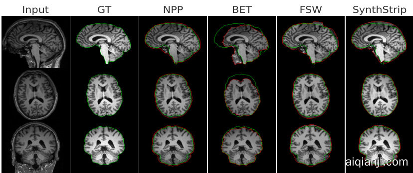
Fig. 2: Representative slices for skull-stripping. From top to bottom: coronal, axial and sagittal views. Green and red contours depict ground truth and estimated brain masks, respectively.

图 2: 颅骨剥离的代表性切片。从上到下：冠状面、轴向面和矢状面视图。绿色和红色轮廓分别表示真实脑掩膜和估计脑掩膜。

$$
\hat{z}{c}=\alpha_{c}z_{c}+\beta_{c},
$$

$$
\hat{z}{c}=\alpha_{c}z_{c}+\beta_{c},
$$

for $c\in{1,...,C}$ . Here, $\alpha_{c}$ and $\beta_{c}$ denote the scale and bias of channel $c$ , conditioned on $\lambda$ . This is repeated for every decoder layer, except the final layer.

对于 $c\in{1,...,C}$。这里，$\alpha_{c}$ 和 $\beta_{c}$ 表示通道 $c$ 的缩放和偏置，其值由 $\lambda$ 决定。该操作在每个解码器层重复进行（最后一层除外）。

3 Experiments

3 实验

Training details. We created a large-scale dataset of 3D T1-weighted (T1w) brain MRI volumes by aggregating 7 datasets: GSP [13], ADNI [21], OASIS [20], ADHD [24], ABIDE [30], MCIC [11], and COBRE [1]. The whole training set contains 10,083 scans. As ground-truth target images, we used FreeSurfer generated skull-stripped, intensity-normalized and affine-registered (to so-called MNI atlas coordinates) images.

训练细节。我们通过整合7个数据集构建了一个大规模3D T1加权(T1w)脑部MRI体素数据集：GSP [13]、ADNI [21]、OASIS [20]、ADHD [24]、ABIDE [30]、MCIC [11]和COBRE [1]。整个训练集包含10,083次扫描。作为真实目标图像，我们采用了FreeSurfer生成的去颅骨、强度归一化且经过仿射配准(至所谓的MNI图谱坐标)的图像。

We train NPP with ADAM [19] and a batch size of 2, for a maximum of 60 epochs. The initial learning rate is 1e-4 and then decreases by half after 30 epochs. We use random gamma transformation as a data augmentation technique, with parameter log gamma (-0.3,0.3). We randomly sampled $\lambda$ from a log-uniform distribution on $(-3,1)$ for each mini-batch.

我们使用ADAM [19]训练NPP，批大小为2，最多60个周期。初始学习率为1e-4，30个周期后减半。采用随机伽马变换作为数据增强技术，参数log gamma (-0.3,0.3)。每个小批量中从$(-3,1)$的对数均匀分布随机采样$\lambda$。

Architecture Details. $f_{\theta}$ is a U-Net-style architecture containing an encoder and decoder with skip connections in between. The encoder and decoder have 5 levels and each level consists of 2 consecutive 3D convolutional layers. Specifically, each 3D convolutional layer is followed by an instance normalization layer and LeakyReLU (negative slope of 0.01). In the bottleneck, we use three transformer blocks to enhance the ability of capturing global information [27]. Each transformer block contains a self-attention layer and a MLP layer. For the transformer block, we use patch size 1x1x1, 8 attention heads, and an MLP expansion ratio of 1. We perform token iz ation by flattening the 3D CNN feature maps into a 1D sequence.

架构细节。$f_{\theta}$ 采用 U-Net 风格架构，包含编码器和解码器，中间通过跳跃连接相连。编码器和解码器各有 5 层，每层由 2 个连续的 3D 卷积层组成。具体而言，每个 3D 卷积层后接一个实例归一化层和 LeakyReLU（负斜率为 0.01）。在瓶颈部分，我们使用三个 Transformer 模块来增强捕获全局信息的能力 [27]。每个 Transformer 模块包含一个自注意力层和一个 MLP 层。对于 Transformer 模块，我们使用 1x1x1 的 patch 大小、8 个注意力头和 MLP 扩展比为 1。我们通过将 3D CNN 特征图展平为一维序列来进行 Token 化。

Table 1: Supported sub-tasks and average runtime for each method. Skullstripping (SS), intensity normalization (IN) and spatial normalization (SN). Units are sec, bold is best.

表 1: 各方法支持的子任务及平均运行时间。颅骨剥离(SS)、强度归一化(IN)和空间归一化(SN)。单位为秒，加粗为最优值。

方法	SS	IN	SN	GPU	CPU
SynthStrip BET Freesurfer	16.5 9.1	- 262.2 747.2 481.5	671.6

Table 2: Performance on intensity normalization. Higher is better, bold is best.

方法	重建SSIM	重建PSNR	偏置SSIM	偏置PSNR
FSL	98.5	34.2	92.5	39.2
FS	98.9	35.7	92.1	39.3
NPP	99.1	36.2	92.7	39.4

表 2: 强度归一化性能对比。数值越高越好，加粗为最优结果。

The hyper network, $h_{\phi}$ , is a 3-layer MLP with hidden layers 512, 2048 and 496. The STN MLP is composed of a global average pooling layer and a 2-layer MLP with hidden layers of size 256 and 12. The 2-layer MLP contains: linear(256 channels); ReLU; linear(12 channels); Tanh. Note an identity matrix is added to the output affine matrix.

超网络 (hyper network) $h_{\phi}$ 是一个包含512、2048和496隐藏层的3层MLP。STN MLP由全局平均池化层和具有256、12隐藏层的2层MLP组成。该2层MLP包含：线性层(256通道)；ReLU激活；线性层(12通道)；Tanh激活。注意输出仿射矩阵会叠加一个单位矩阵。

Baselines. We chose three popular and widely-used tools, SynthStrip [15], FSL [25], and FreeSurfer [9], as baselines. SynthStrip (SS) is a learning-based skull-stripping method, while FSL and FreeSurfer (FS) is a cross-platform brain processing package containing multiple tools. FSL’s Brain Extraction Tool (BET) and FMRIB’s Automated Segmentation Tool are for skull stripping and MR bias field correction, respectively. FS uses a watershed method for skull-stripping, a model-based tissue segmentation for intensity normalization and bias field correction.

基线方法。我们选择了三种流行且广泛使用的工具作为基线：SynthStrip [15]、FSL [25] 和 FreeSurfer [9]。SynthStrip (SS) 是一种基于学习的颅骨剥离方法，而 FSL 和 FreeSurfer (FS) 是包含多种工具的跨平台脑处理套件。FSL 的脑提取工具 (BET) 和 FMRIB 的自动分割工具分别用于颅骨剥离和 MR 偏置场校正。FS 采用分水岭法进行颅骨剥离，并基于模型的组织分割实现强度归一化和偏置场校正。

3.1 Runtime analyses

3.1 运行时分析

The primary advantage of NPP is runtime. As shown in Table 1, for images with resolution $256\times256\times256$ , NPP requires less than 3 sec on a GPU and less than 8 sec on a CPU for all three pre-processing tasks. This is in part due to the fact that the multiplier field can be computed at a lower resolution (in our case, on a grid of $128\times128\times128$ ). The output field is then up-sampled with trilinear interpolation before being multiplied with the input image. In contrast, SynthStrip needs 16.5 sec on a GPU for skull stripping. FSL’s optimized implementation takes about 271.3 sec per image for skull stripping and intensity normalization, whereas FreeSurfer needs more than 10 min.

NPP的主要优势在于运行时间。如表 1 所示，对于分辨率为 $256\times256\times256$ 的图像，NPP在GPU上完成所有三项预处理任务耗时不足3秒，在CPU上也不超过8秒。这部分归功于乘数字段可在较低分辨率下计算（本实验采用 $128\times128\times128$ 网格）。输出字段经三线性插值上采样后，再与输入图像相乘。相比之下，SynthStrip在GPU上进行颅骨剥离需16.5秒，FSL的优化实现完成颅骨剥离和强度标准化约需271.3秒/图像，而FreeSurfer则需耗时10分钟以上。

3.2 Pre-processing Performance

3.2 预处理性能

We empirically validate the performance of NPP for the three tasks we consider: skull-stripping, intensity normalization, and spatial transformation.

我们通过实验验证了NPP在颅骨剥离、强度归一化和空间变换这三个任务上的性能。

Fig. 3: Skull-stripping performance on various metrics. (Top) Higher is better. (Bottom) Lower is better.

图 3: 不同指标下的颅骨剥离性能。(上) 数值越高越好。(下) 数值越低越好。

Evaluation Datasets. For skull-stripping, we evaluate on the Neural feedback skull-stripped repository (NFSR) [7] dataset. NFSR contains 125 manually skullstripped T1w images from individuals aged 21 to 45, and are diagnosed with a wide range of psychiatric diseases. The definition of the brain mask used in NFSR follows that of FS. For intensity normalization, we evaluate on the test set (N=856) from the Human Connectome Project (HCP). The HCP dataset includes T1w and T2w brain MRI scans which can be combined to obtain a high quality estimate of the bias field [26,10]. For spatial normalization, we use T1w MRI scans from the Parkinson’s Progression Markers Initiative (PPMI). These images were automatically segmented using Freesurfer into anatomical regions of interest (ROIs) $^3$ [6].

评估数据集。对于颅骨剥离任务，我们在神经反馈颅骨剥离资源库 (NFSR) [7] 数据集上进行评估。NFSR包含125例21至45岁个体的手动颅骨剥离T1加权图像，这些个体被诊断患有多种精神疾病。NFSR中使用的脑掩膜定义与FS一致。对于强度归一化任务，我们使用人类连接组计划 (HCP) 的测试集 (N=856) 进行评估。HCP数据集包含T1加权和T2加权脑部MRI扫描，可结合二者获得高质量的偏置场估计 [26,10]。对于空间归一化任务，我们使用帕金森病进展标志物计划 (PPMI) 的T1加权MRI扫描。这些图像已通过Freesurfer自动分割为感兴趣解剖区域 (ROIs) $^3$ [6]。

Metrics. For skull-stripping, we quantify performance using the Dice overlap coefficient (Dice), Sensitivity (Sens), Specificity (Spec), mean surface distance (MSD), residual mean surface distance (RMSD), and Hausdorff distance (HD), as defined elsewhere [18]. For intensity normalization, we evaluate the intensitynormalized reconstruction (Rec) and estimated bias image (Bias, which is equal to the multiplier field $\chi$ ) to the ground truth images, using PSNR and SSIM. For spatial normalization, we quantify performance by the Dice score between the spatially transformed segmentation s (resampled using the estimated affine transformation) and the probabilistic labels of the target atlas.

指标。对于颅骨剥离任务，我们采用以下指标量化性能：Dice重叠系数 (Dice)、灵敏度 (Sens)、特异度 (Spec)、平均表面距离 (MSD)、残差平均表面距离 (RMSD) 和豪斯多夫距离 (HD)，具体定义见文献 [18]。在强度归一化评估中，我们通过峰值信噪比 (PSNR) 和结构相似性 (SSIM) 来评估强度归一化重建图像 (Rec) 和估计偏置场图像 (Bias，即乘数场 $\chi$ ) 与真实图像的差异。空间归一化性能则通过空间变换后的分割结果 s (使用估计的仿射变换进行重采样) 与目标图谱概率标签之间的 Dice 分数来量化。

Results. Fig 2 and Fig 3 shows skull-stripping performance for all models. We observe that the proposed method outperforms all traditional and learningbased baselines on Dice, Spec, and MSD/RMSD. Importantly, NPP achieved

结果。图2和图3展示了所有模型的颅骨剥离性能。我们观察到，所提出的方法在Dice、Spec和MSD/RMSD指标上均优于所有传统和基于学习的基线方法。值得注意的是，NPP实现了

Fig. 4: (a) Representative examples for spatial normalization. Rows depict sagittal, axial and coronal view. For each view, from left to right: input image, atlas, NPP results, and FreeSurfer results. (b) Boxplots illustrating Dice scores of each anatomical structure for NPP and FreeSurfer in the atlas-based registration with the PPMI dataset. We combine left and right hemispheres of the brain into one structure for visualization.

图 4: (a) 空间归一化的代表性示例。行分别表示矢状面、轴向和冠状面视图。每种视图中从左到右依次为: 输入图像、图谱、NPP处理结果和FreeSurfer处理结果。(b) 箱线图展示了NPP和FreeSurfer在基于PPMI数据集的图谱配准中，各解剖结构的Dice分数。为便于可视化，我们将大脑左右半球合并为一个结构进行展示。

$93.8%$ accuracy and 2.7% improvement on Dice and 2.39mm MSD. Especially for MSD, NPP is 28% better than the second-best method, SynthStrip. We further observe that BET commonly fails, which has also been noted in the literature [8].

准确率达到93.8%，Dice系数提升2.7%，MSD指标改善2.39毫米。尤其在MSD指标上，NPP方法比第二名SynthStrip方法表现优异28%。我们还发现BET方法普遍失效，这一现象在文献[8]中也有记载。

Table 2 shows the quantitative results of FSL, FS and NPP(see visualization results in Supplementary S1). NPP outperforms the baselines on all metrics. From Table 2, we see that FreeSurfer’s reconstruction is better than BET’s, but the bias field estimates are relatively worse. We can appreciate this in the figure in Supplementary S1, as we observe that FS’s bias field estimate (f) contains too much high-frequency anatomical detail.

表 2 展示了 FSL、FS 和 NPP 的定量结果 (可视化结果见补充材料 S1)。NPP 在所有指标上均优于基线方法。从表 2 可以看出，FreeSurfer 的重建效果优于 BET，但其偏置场估计相对较差。这一点在补充材料 S1 的图中尤为明显，我们观察到 FS 的偏置场估计 (f) 包含了过多高频解剖细节。

Fig. 4 (b) shows boxplots of Dice scores for NPP and FreeSurfer, for each ROI. Compared to FS, NPP achieves consistent improvement on all ROIs measured. Fig. 4 (a) shows representative slices for spatial normalization.

图4 (b) 展示了NPP和FreeSurfer在各ROI区域的Dice分数箱线图。与FS相比，NPP在所有测量ROI上都实现了稳定提升。图4 (a) 显示了空间归一化的代表性切片。

Table 3: Ablation study results of different $\lambda$ . Bold is best.

表 3: 不同 $\lambda$ 的消融研究结果。加粗表示最佳。

方法	RecSSIM	BiasSSIM
NPP, $\lambda$=10	96.38±1.29	96.02±1.29
NPP, $\lambda$=1	99.07±0.61	98.09±0.62
NPP, $\lambda$=0.1	99.25±0.52	98.40±0.40

Table 4: Comparison with ablated models. Bold is best.

表 4: 消融模型对比。粗体表示最佳结果。

方法	RecSSIM
Naive U-Net	84.12±3.34
U-Net+STN	84.87±3.04
UMIRGPIT	84.26±3.02
NPP, λ=0.1	99.25±0.52

Fig. 5: (Top) From left to right, raw input image, ground truth bias field, estimated multiplier fields from NPP for different values of $\lambda=10,1,0.1,0.01,0.001$ . (Bottom) From left to right, ground truth, outputs from NPP for different values of $\lambda$ .

图 5: (上排) 从左至右分别为: 原始输入图像、真实偏置场 (ground truth bias field)、NPP在不同$\lambda=10,1,0.1,0.01,0.001$值下估计的乘数场 (estimated multiplier fields)。(下排) 从左至右分别为: 真实值 (ground truth)、NPP在不同$\lambda$值下的输出结果。

3.3 Ablation

3.3 消融实验

As ablations, we compare the specialized architecture of NPP against a naive U-Net trained to solve all three tasks at once. Additionally, we implemented a different version of our model where the U-Net directly outputs the skullstripped and intensity-normalized image, which is in turn re-sampled with the STN. In this version, we did not have the scalar multiplication field and thus our loss function did not include the total variation term. We call this version U-Net $^+$ STN. As another alternative, we trained the U-Net $^+$ STN architecture via UMIRGPIT [2], which encourages the translation network (U-Net) to be geometry-preserving by alternating the order of the translation and registration. We note again that for all these baselines, we used the same architecture as $f_{\theta}$ , but instead of computing the multiplier field $\chi$ , $f_{\theta}$ computes the final intensity-normalized and spatially transformed image directly. The objective is the reconstruction loss $L_{r e c}$ . All other implementation details were the same as NPP. For evaluation, we use the test images from the HCP dataset.

作为消融实验，我们将NPP的专用架构与同时训练解决所有三个任务的朴素U-Net进行对比。此外，我们还实现了模型的另一个版本，其中U-Net直接输出经颅骨剥离和强度归一化的图像，再由STN进行重采样。该版本未包含标量乘法场，因此损失函数不包含总变差项。我们将此版本称为U-Net $^+$ STN。作为另一种替代方案，我们通过UMIRGPIT [2]训练U-Net $^+$ STN架构，该方法通过交替执行配准与转换的顺序，促使转换网络(U-Net)保持几何特性。需要再次说明的是，所有基线模型均采用与$f_{\theta}$相同的架构，但$f_{\theta}$直接计算最终强度归一化且空间转换后的图像，而非计算乘法场$\chi$。目标函数为重建损失$L_{rec}$。其余实现细节均与NPP保持一致。评估阶段我们使用HCP数据集的测试图像。

Results: Tables 3 and 4 lists the SSIM values for the estimated reconstruction and bias fields, for different ablations and NPP with a range of $\lambda$ values. We observe that there is a sweet spot around $\lambda=0.1$ , which underscores the importance of considering different hyper parameter settings and affording the user to optimize this at test time. All ablation results are poor, supporting the importance of our architectural design. Fig. 5 shows some representative results for a range of $\lambda$ values.

结果：表3和表4列出了不同消融实验和NPP在不同$\lambda$值下估计重建与偏置场的SSIM值。我们观察到$\lambda=0.1$附近存在最佳平衡点，这凸显了考虑不同超参数设置并允许用户在测试时优化该参数的重要性。所有消融实验结果均较差，证实了我们架构设计的关键性。图5展示了一组$\lambda$值下的代表性结果。

4 Conclusion

4 结论

In this paper, we propose a novel neural network approach for brain MRI preprocessing. The proposed model, called NPP, disentangles geometry-preserving translation mapping (which includes skull stripping and bias field correction) and spatial transformation. Our experiments demonstrate that NPP can achieve state-of-the-art results for the major tasks of brain MRI pre-processing.

本文提出了一种用于脑部MRI预处理的新型神经网络方法。该模型名为NPP，能够解耦保持几何形状的平移映射（包括颅骨剥离和偏置场校正）与空间变换。实验表明，NPP在脑部MRI预处理的主要任务上可以达到最先进的结果。

Fig. 6: Representative slices of intensity normalization performance on HCP T1w brain images. (a) input image; (b-d) intensity normalized outputs from FreeSurfer, FSL, and NPP with $\lambda=0.1$ ; (e) ground truth bias field; (f-h) bias fields estimated by the corresponding methods; (i) ground-truth intensity normalized image; (j-l) prediction error maps corresponding to (b-d).

图 6: HCP T1w脑图像强度归一化性能的代表性切片。(a) 输入图像；(b-d) FreeSurfer、FSL和NPP (λ=0.1)的强度归一化输出；(e) 真实偏置场；(f-h) 对应方法估计的偏置场；(i) 真实强度归一化图像；(j-l) 与(b-d)对应的预测误差图。