Pair-VPR: Place-Aware Pre-training and Contrastive Pair Classification for Visual Place Recognition with Vision Transformers
Pair-VPR: 基于位置感知预训练和对比配对分类的视觉位置识别方法(Vision Transformers)
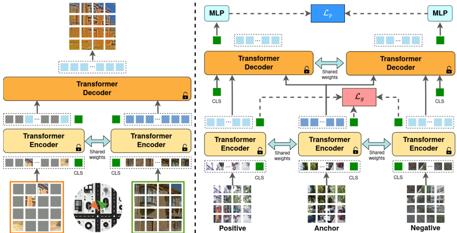
Fig. 1: Overview of the proposed Pair-VPR method. Left: In Stage 1 of training, we train a ViT encoder and decoder using Siamese mask image modelling with place-aware image sampling. Right: In Stage 2, we re-use the pre-trained encoder and decoder and train specifically for the VPR task, jointly learning a global descriptor and a pair classifier.
图 1: 提出的Pair-VPR方法概述。左: 在训练的第一阶段,我们使用带有位置感知图像采样的Siamese掩码图像建模来训练ViT编码器和解码器。右: 在第二阶段,我们复用预训练的编码器和解码器,专门针对VPR任务进行训练,联合学习全局描述符和配对分类器。
Abstract—In this work we propose a novel joint training method for Visual Place Recognition (VPR), which simultaneously learns a global descriptor and a pair classifier for reranking. The pair classifier can predict whether a given pair of images are from the same place or not. The network only comprises Vision Transformer components for both the encoder and the pair classifier, and both components are trained using their respective class tokens. In existing VPR methods, typically the network is initialized using pre-trained weights from a generic image dataset such as ImageNet. In this work we propose an alternative pre-training strategy, by using Siamese Masked Image Modeling as a pre-training task. We propose a Place-aware image sampling procedure from a collection of large VPR datasets for pre-training our model, to learn visual features tuned specifically for VPR. By re-using the Mask Image Modeling encoder and decoder weights in the second stage of training, Pair-VPR can achieve state-of-the-art VPR performance across five benchmark
摘要—本文提出了一种新颖的视觉位置识别(VPR)联合训练方法,该方法同时学习全局描述符和用于重排序的图像对分类器。该分类器可预测给定图像对是否来自同一地点。网络仅由Vision Transformer组件构成,包括编码器和图像对分类器,两者均使用各自的类别token进行训练。现有VPR方法通常使用通用图像数据集(如ImageNet)的预训练权重初始化网络。本文提出了一种替代预训练策略,采用孪生掩码图像建模(Siamese Masked Image Modeling)作为预训练任务。我们提出从大型VPR数据集中进行位置感知图像采样的方法,以预训练专门针对VPR任务优化的视觉特征模型。通过在第二阶段训练中复用掩码图像建模的编码器和解码器权重,Pair-VPR在五个基准测试中实现了最先进的VPR性能。
Manuscript received: Oct 3, 2024; Revised Jan 12, 2025; Accepted Feb 13, 2025. This paper was recommended for publication by Editor Sven Behnke upon evaluation of the Associate Editor and Reviewers’ comments. This work was supported by the CSIRO’s Data61 Embodied AI Cluster.
稿件收稿日期:2024年10月3日;修改日期:2025年1月12日;录用日期:2025年2月13日。本文由副编辑和审稿人评审后,经Sven Behnke编辑推荐发表。本工作得到了CSIRO Data61 Embodied AI集群的支持。
1 CSIRO Robotics, Data61, CSIRO, Brisbane, QLD, Australia. E-mail: peyman.moghadam@csiro.au † This work was done while the author was at CSIRO. 2 School of Electrical Engineering and Robotics, Queensland University of Technology (QUT), Brisbane, Australia.
1 澳大利亚联邦科学与工业研究组织(CSIRO)机器人研究所,Data61,布里斯班,QLD。邮箱:peyman.moghadam@csiro.au † 本工作完成时作者任职于CSIRO。
2 昆士兰科技大学(QUT)电气工程与机器人学院,澳大利亚布里斯班。
datasets with a ViT-B encoder, along with further improvements in localization recall with larger encoders. The Pair-VPR website is: https://csiro-robotics.github.io/Pair-VPR
使用ViT-B编码器的数据集,以及更大编码器在定位召回率上的进一步改进。Pair-VPR网站为:https://csiro-robotics.github.io/Pair-VPR
Index Terms—Deep Learning for Visual Perception; Recognition; Localization
视觉感知深度学习;识别;定位
I. INTRODUCTION
I. 引言
HE Place Recognition (PR) task involves associating T input sensor data (e.g., lidar [1], radar [2], or vision [3]), with a global map or database of places previously visited within an environment. In the field of learning-based Visual Place Recognition (VPR) [3], [4], it is a standard approach to start with a pre-trained neural network, such as VGG16 or ResNet, leveraging their initial architecture and weights for the VPR task. Following this, it is common to incorporate a feature aggregation layer — such as VLAD [5], GeM [6], Conv-AP [7], SoP [1] among others — to pool local features into a compact global descriptor vector efficiently representing the original image. These vectors can then be compared with an embedding distance metric such as the Euclidean distance, with the smallest distance noting the pair of most similar images. More recent VPR techniques often include multiple stages of retrieval, where subsequent stages of retrieval are used to re-rank an initial set of candidate place recognition matches [8]–[11].
地点识别 (PR) 任务涉及将输入传感器数据 (如激光雷达 [1]、雷达 [2] 或视觉 [3]) 与环境内先前访问过的全局地图或地点数据库关联。在基于学习的视觉地点识别 (VPR) [3][4] 领域,标准做法是从预训练神经网络 (如 VGG16 或 ResNet) 开始,利用其初始架构和权重进行 VPR 任务。随后通常会引入特征聚合层 (如 VLAD [5]、GeM [6]、Conv-AP [7]、SoP [1] 等),将局部特征池化为紧凑的全局描述符向量,从而高效表征原始图像。这些向量可通过嵌入距离度量 (如欧氏距离) 进行比较,最小距离对应最相似的图像对。最新 VPR 技术通常包含多阶段检索,其中后续检索阶段用于对初始候选地点识别匹配集进行重排序 [8]–[11]。
In this work, we develop Pair-VPR, a transformer-based VPR method trained on diverse VPR datasets, which achieves state-of-the-art visual place recognition performance across a range of challenging VPR benchmarks. We achieve this by proposing a two-stage training pipeline to train a pairclassifier, which can decide whether a given pair of images is from the same place or not. In the first stage, we pre-train a transformer encoder and decoder using Siamese mask image modeling [12], [13], with place-aware image sampling. We sample pairs of images from different places in the world, ensuring that these pairs contain both spatial and temporal differences. Our places are curated from three existing largescale open source datasets (SF-XL [14], GSV-Cities [7] and Google Landmarks v2 [15]) with a total of 3.43 million panoramic images and 2.08 million egocentric images, across diverse locations (planet-wide) and diverse times.
在本工作中,我们开发了Pair-VPR,这是一种基于Transformer的视觉地点识别方法,通过在多组VPR数据集上训练,在一系列具有挑战性的VPR基准测试中实现了最先进的性能。我们通过提出一个两阶段训练流程来训练一个配对分类器,该分类器可以判断给定的图像对是否来自同一地点。在第一阶段,我们使用孪生掩码图像建模[12][13]和地点感知图像采样,预训练了一个Transformer编码器和解码器。我们从世界各地的不同地点采样图像对,确保这些图像对包含空间和时间上的差异。我们的地点数据来自三个现有的大规模开源数据集(SF-XL[14]、GSV-Cities[7]和Google Landmarks v2[15]),总计包含343万张全景图像和208万张以自我为中心的图像,涵盖了全球不同地点和不同时间段。
In the second stage, we re-use both the encoder and decoder, by jointly learning to produce a global descriptor from the encoder and using the decoder as a pair classification network. The pair classifier produces a similarity score denoting whether a given pair of images were captured from the same location, or not. A diagram showing our network architecture and training recipe is shown in Figure 1. The Pair-VPR network uses a vision transformer setup, with ViT blocks in both the encoder and decoder. We leverage the class token output to supervise the network, with a low-dimensional global descriptor produced from an encoder class token and a pair similarity score from decoder class tokens. The network is then trained using a Multi-Similarity loss for the global descriptor and a Binary Cross-Entropy loss for the pair classifier, with online triplet mining. We benchmark the trained network on existing VPR benchmark datasets and observe state-of-the-art Recall $@1$ on all tested datasets with a ViT-B encoder, such as an improvement in the Recall $@1$ on the Tokyo24/7 dataset from $95%$ to $98%$ . Moreover, we show that our proposed method can be extended to much larger vision transformer encoders (ViT-L, ViT-G) and achieve a new benchmark result of Recall $@1$ on Tokyo24/7 of $100%$ with our best performing configuration.
在第二阶段,我们复用编码器和解码器,通过联合学习从编码器生成全局描述符,并将解码器用作配对分类网络。配对分类器生成相似度分数,表示给定图像对是否拍摄于同一地点。图1展示了我们的网络架构和训练方案。Pair-VPR网络采用视觉Transformer (ViT) 架构,编码器和解码器均使用ViT模块。我们利用类别Token输出来监督网络,其中编码器类别Token生成低维全局描述符,解码器类别Token输出配对相似度分数。网络训练时采用多相似度损失函数优化全局描述符,使用二元交叉熵损失函数结合在线三元组挖掘训练配对分类器。在现有VPR基准数据集上测试表明,采用ViT-B编码器时所有测试数据集均达到最优的召回率$@1$,例如Tokyo24/7数据集的召回率$@1$从$95%$提升至$98%$。此外,我们证明该方法可扩展至更大规模的视觉Transformer编码器(ViT-L、ViT-G),在最优配置下将Tokyo24/7数据集的召回率$@1$提升至$100%$,创下新基准记录。
II. RELATED WORK
II. 相关工作
A. Visual Place Recognition
A. 视觉地点识别
Compared to the general task of Place Recognition, VPR focuses only on the image modality and this allows for VPR to be considered as an image retrieval problem. This formulation in conjunction with the advent of deep learning led to a number of high performing learning-based VPR solutions. Initially, pre-trained neural networks were applied to VPR, then NetVLAD was developed which utilized triplet loss to train a neural network specifically for the place recognition task [3]. Numerous subsequent works expanded upon NetVLAD, including works that relax the triplet loss to use soft positives and negatives [16], quadruplets rather than triplets [17], a generalized contrastive loss [18], and aggregates features over multiple spatial scales [19]. Other learning-based methods include those which consider place recognition as a classification problem [4], [14] or use a multisimilarity loss [20]. These earlier works all follow the same approach, of constructing a global descriptor, i.e., a single vector representing an image for nearest neighbor retrieval. However, the top candidate found using global descriptor matching is not always correct. To avoid such limitations, multi-stage VPR algorithms propose to re-rank a collection of top candidates.
与通用的地点识别任务相比,视觉地点识别(VPR)仅关注图像模态,这使得VPR可以被视为图像检索问题。这一形式化定义与深度学习的兴起共同催生了许多高性能的基于学习的VPR解决方案。最初,预训练神经网络被应用于VPR,随后NetVLAD开发出来,它利用三元组损失(triplet loss)专门针对地点识别任务训练神经网络[3]。后续大量工作在NetVLAD基础上进行扩展,包括放宽三元组损失以使用软正负样本[16]、采用四元组而非三元组[17]、提出广义对比损失[18]、以及聚合多空间尺度特征[19]等方法。其他基于学习的方法包括将地点识别视为分类问题[4][14]或使用多重相似度损失[20]的解决方案。这些早期研究都遵循相同的方法论,即构建全局描述符(即代表图像的单向量)用于最近邻检索。然而,使用全局描述符匹配得到的最佳候选结果并不总是正确的。为避免这种局限性,多阶段VPR算法提出对一组顶级候选结果进行重新排序。
These re-ranking methods involve re-ordering an initial set of retrieved places such that the correct place match is ranked first in the retrieved list. Learning-based re-ranking methods began with less computationally efficient algorithms that used geometric verification densely (without keypoint selection) [9], then subsequently evolved to include keypoint/keypatch selection algorithms [10], [21]. More recently, R2Former [22] went one step further by removing explicit geometric verification altogether. Instead, they treat re-ranking as a classification problem and use a small two-block transformer for selecting the best candidate image. Similarly, GeoAdapt [23] also learns a classifier except instead for the task of classifying the similarity of two point clouds for LiDAR Place Recognition. In our proposed approach, we show that a re-ranking classification transformer can be designed using standard self and crossattention blocks and scaled up to over 80 million parameters, by leveraging a VPR-specific pre-training recipe.
这些重排序方法涉及对初始检索到的地方进行重新排序,使得正确的地点匹配在检索列表中排名第一。基于学习的重排序方法最初采用计算效率较低的算法,这些算法密集使用几何验证(无需关键点选择)[9],随后发展为包含关键点/关键块选择算法[10][21]。最近,R2Former[22]更进一步,完全移除了显式的几何验证,而是将重排序视为分类问题,并使用一个小的两模块Transformer来选择最佳候选图像。类似地,GeoAdapt[23]也学习了一个分类器,但用于LiDAR地点识别中两个点云相似性的分类任务。在我们提出的方法中,我们展示了通过利用专门针对视觉地点识别(VPR)的预训练方案,可以使用标准的自注意力和交叉注意力模块设计一个重排序分类Transformer,并将其扩展到超过8000万个参数。
B. Vision Transformers and Self-Supervised Learning
B. Vision Transformer和自监督学习
Compared to Convolutional Networks (CNNs), Vision Transformers [24] have no inductive bias therefore they can learn global dependencies between image features without being limited by a specific kernel size; however, as a result, larger image datasets are needed to train transformer models. This led to the concept of Self-Supervised Learning (SSL) techniques for pre-training these large transformer models on large quantities of unlabeled data. These techniques include deep metric learning methods such as SimCLR [25], BYOL [26], and DINO [27]. The recent work DINOv2 [28] provided further improvements to the pre-training recipe and in this work, we leverage the robust learnt features they provide. In contrast to metric learning methods, an alternate self-supervised approach is called Masked Image Modeling (MIM) and will be explained in the following subsection.
与卷积网络(CNN)相比,Vision Transformer [24] 没有归纳偏置(inductive bias),因此可以学习图像特征之间的全局依赖关系,而不受特定卷积核大小的限制;但这也意味着需要更大的图像数据集来训练Transformer模型。这催生了自监督学习(SSL)技术概念,用于在大量无标注数据上预训练这些大型Transformer模型。相关技术包括SimCLR [25]、BYOL [26] 和DINO [27] 等深度度量学习方法。近期工作DINOv2 [28] 进一步改进了预训练方案,本研究正是利用了其提供的鲁棒性学习特征。与度量学习方法不同,另一种自监督方法称为掩码图像建模(MIM),我们将在下一小节详细说明。
C. Masked Image Modeling (MIM) and Siamese MIM
C. 掩码图像建模 (Masked Image Modeling, MIM) 与孪生 MIM (Siamese MIM)
Masked Image Modeling is a SSL technique where a neural network is tasked with reconstructing a partially masked image, where the image is divided into a set of non-overlapping patches. Initially, this reconstruction was performed on a set of transformer tokens produced from a raw image [29]. Subsequently, MAE [30] demonstrated that instead the reconstruction could be performed directly on the raw pixel values, based on the mean squared pixel error between the original and reconstructed image. Further works then expanded upon this concept via improvements such as distillation (iBOT [31]), continuous masking (ROPIM [32]), and cross-view completion (CroCo [13]). In CroCo, pairs of images are provided to the network where one image is masked and a second image, showing the same scene, is provided to the network without any masking. They showed that this pre-training recipe is ideal for 3D vision tasks. In a concurrent work, a similar architecture was proposed for learning from video data, called Siamese Masked Auto encoders [12]. In our approach, we also provide pairs of images to a Mask Image Modeling network, except we propose a Place-aware training methodology for VPR.
掩码图像建模 (Masked Image Modeling) 是一种自监督学习技术,其任务是让神经网络重建部分被掩码的图像。该技术将图像划分为一组不重叠的图块,最初是在原始图像生成的Transformer token集合上进行重建 [29]。随后,MAE [30] 证明可以直接基于原始像素值与重建图像之间的均方像素误差进行重建。后续研究通过改进进一步扩展了这一概念,例如蒸馏 (iBOT [31])、连续掩码 (ROPIM [32]) 和跨视角补全 (CroCo [13])。在CroCo中,网络接收成对的图像,其中一张图像被掩码,另一张显示同一场景的图像则完全未被掩码。研究表明,这种预训练方案非常适合3D视觉任务。在同期工作中,有人提出了类似架构用于从视频数据中学习,称为孪生掩码自编码器 (Siamese Masked Autoencoders) [12]。在我们的方法中,我们也向掩码图像建模网络提供成对图像,但针对视觉位置识别 (VPR) 提出了一种位置感知训练方法。
III. METHODOLOGY
III. 方法论
Our proposed Visual Place Recognition (Pair-VPR) solution is a two-stage place recognition method, which first uses a global descriptor to generate a list of potential place matches, then uses a second stage to refine these matches to improve the likelihood that the highest ranked match is correct. For the first time, we propose a two-stage training methodology using a mask image modeling pre-training designed specifically for VPR. Then we propose a second stage approach where we learn to generate both a global descriptor and a pair classifier for VPR.
我们提出的视觉位置识别方案(Pair-VPR)是一种两阶段位置识别方法:首先使用全局描述符生成潜在位置匹配列表,随后通过第二阶段优化这些匹配以提高最高排名匹配的正确概率。我们首次提出采用专为VPR设计的掩码图像建模预训练进行两阶段训练,继而提出在第二阶段同时学习生成全局描述符和配对分类器的创新方法。
During the first stage, we provide pairs of images to the network and then heavily mask one of these images. The training objective is to reconstruct the masked image, using a network that has both encoder and decoder components. In the second stage we jointly optimize both the encoder and decoder for VPR, generating a global descriptor from the class token of the encoder, and the decoder is trained to predict whether a given pair of images is a positive or negative pair.
在第一阶段,我们向网络提供图像对,并对其中一张图像进行重度掩码处理。训练目标是通过具备编码器和解码器组件的网络重构被掩码图像。在第二阶段,我们联合优化编码器和解码器以用于视觉位置识别 (VPR),从编码器的类别 token 生成全局描述符,同时训练解码器预测给定图像对是正样本对还是负样本对。
After training, the network can then be used as a two-stage VPR method. The encoder is used to produce low dimensional global descriptors which are then used for nearest neighbor searching through a VPR database. Then the decoder is used to decide which potential database candidate is the best match for the current query by passing (query, database) pairs to the decoder. An overview of our pre-training and fine-tuning procedures are provided in Figure 1.
训练完成后,该网络可作为两阶段VPR方法使用。编码器用于生成低维全局描述符,随后通过VPR数据库进行最近邻搜索。解码器则通过传递(查询,数据库)对来决定哪个潜在数据库候选与当前查询最匹配。图1展示了我们的预训练和微调流程概览。
A. Stage One: Place-Aware Masked Image Modeling
A. 第一阶段:位置感知掩码图像建模 (Place-Aware Masked Image Modeling)
In the first stage of training, we use the Siamese Masked Auto encoder [12] design to train the Pair-VPR network. In this approach, pairs of images are input into the network, and one of the images is heavily masked. The network is then able to leverage the visual information in the second, unmasked image to aid in reconstructing the masked first image. In previous works, generating pairs is achieved either by sampling random frames in a video sequence [12], or by sampling two different viewpoints of a scene [13]. In our approach, we propose a location sampling strategy, such that pairs are sampled from specific locations and, in VPR terminology, are always collected from the set of positives from a given place.
在训练的第一阶段,我们采用Siamese Masked Auto encoder [12] 设计来训练Pair-VPR网络。该方法将成对的图像输入网络,其中一张图像被严重遮挡。网络能够利用第二张未遮挡图像中的视觉信息来辅助重建被遮挡的第一张图像。在先前工作中,生成图像对的方法包括从视频序列中随机采样帧 [12] 或从场景的两个不同视角采样 [13]。本研究中,我们提出了一种位置采样策略,即从特定位置采样图像对,用VPR术语来说,这些样本始终来自给定地点的正样本集。
Network: Our network comprises a shared encoder that converts a first image $I_{a}$ (masked) and a second image $I_{b}$ (unmasked) into latent representations. We use a Vision Transformer [24] encoder and convert each image into a collection of non-overlapping patches, which are then converted to a set of tokens. For the masked image, we replace the majority of image tokens with mask tokens, which are learnt parameters but have no information received from the original image.
网络:我们的网络包含一个共享编码器,用于将第一张图像 $I_{a}$(掩码处理)和第二张图像 $I_{b}$(未掩码)转换为潜在表示。我们采用 Vision Transformer [24] 编码器,将每张图像转换为一系列不重叠的图块,随后再转换为一组 Token。对于掩码图像,我们将大部分图像 Token 替换为掩码 Token(这些是学习得到的参数,但不包含来自原始图像的任何信息)。
After the encoder, we pass the set of encoded patch embeddings (excluding any class tokens) from both images through a decoder to reconstruct the masked image. Our decoder consists of another vision transformer except with alternating self-attention and cross-attention layers, with self-attention between tokens from $I_{a}$ and cross-attention between tokens from $I_{a}$ and $I_{b}$ . For efficiency, we use Flash Attention [33]. After a number of decoder blocks, we pass the features through a final FC layer to produce reconstructed pixel values per token (i.e., per image patch).
在编码器之后,我们将两组图像的编码补丁嵌入(不包括任何类别token)通过解码器传递以重建被遮蔽的图像。我们的解码器由另一个视觉Transformer组成,但采用了交替的自注意力层和交叉注意力层——其中自注意力作用于$I_{a}$的token之间,而交叉注意力作用于$I_{a}$与$I_{b}$的token之间。为提高效率,我们使用了Flash Attention [33]。经过若干解码器块后,我们将特征通过最终的FC层,为每个token(即每个图像补丁)生成重建的像素值。
Loss: The network is trained using a reconstruction loss between the predicted and ground truth (unmasked) images, by minimizing the Mean Squared Error between predicted and true pixel values. The loss function is expressed as below:
损失函数:网络通过最小化预测像素值与真实像素值之间的均方误差,使用预测图像与真实(未掩码)图像之间的重建损失进行训练。损失函数表达式如下:
$$
\mathcal{L}\left(I_{a},I_{b}\right)=\frac{1}{|p_{a}/\tilde{p}{a}|}\sum_{p_{a}^{i}\in p_{a}/\tilde{p}{a}}||\hat{p}{a}^{i}-p_{a}^{i}||^{2},
$$
$$
\mathcal{L}\left(I_{a},I_{b}\right)=\frac{1}{|p_{a}/\tilde{p}{a}|}\sum_{p_{a}^{i}\in p_{a}/\tilde{p}{a}}||\hat{p}{a}^{i}-p_{a}^{i}||^{2},
$$
where $I_{a}$ and $I_{b}$ denote the two input images, $p_{a}$ denotes the ground truth value for a masked pixel at index $i$ from image $I_{a}$ , $\hat{p}{a}$ denotes the predicted pixel value, and $p_{a}/\tilde{p}_{a}$ is the subset of masked pixels from the masked image. The loss function is only calculated for any pixels that have been masked, where the mask ratio is a hyper parameter of the network. Before calculating the loss we normalize each patch by the mean and standard deviation of that patch as per prior work [30].
其中 $I_{a}$ 和 $I_{b}$ 表示两张输入图像,$p_{a}$ 表示图像 $I_{a}$ 中索引为 $i$ 的掩码像素的真实值,$\hat{p}{a}$ 表示预测像素值,$p_{a}/\tilde{p}_{a}$ 是掩码图像中掩码像素的子集。损失函数仅针对被掩码的像素进行计算,其中掩码比例是网络的超参数。在计算损失之前,我们按照先前工作 [30] 的方法对每个图像块进行均值和标准差归一化。
Training: Our network is pre-trained in a Place-aware fashion, where each iteration is a defined physical location in the world. Then pairs of images are sampled from this place, with dataset-specific sampling to ensure that sampled pairs have some viewpoint consistency; it would be almost impossible for the network to reconstruct an image using a second image facing the opposite direction. Our training data can theoretically be drawn from any collection of places in the world, however, in this work we limit ourselves to a set of pre-existing open-source datasets. Further details concerning dataset specific implementations are provided in Section Four.
训练:我们的网络采用位置感知 (Place-aware) 方式进行预训练,每次迭代对应现实世界中一个明确的物理位置。随后从该位置采样图像对,并通过数据集特定的采样机制确保成对图像具有视角一致性(若第二张图像朝向完全相反的方向,网络几乎无法完成重建)。理论上训练数据可来自全球任意地点集合,但本文仅使用一组现有开源数据集。具体数据集实现细节详见第四节。
B. Stage Two: Contrastive Pair Classification for VPR
B. 第二阶段:基于对比对分类的视觉位置识别 (VPR)
In the second stage, the encoder is trained to generate global descriptors for retrieval, and the decoder is trained to predict whether a given pair of images is similar or not. We used the pre-trained weights from stage one of Pair-VPR, loading weights from both the encoder and the mask image modeling decoder. We then jointly train the encoder and decoder for both global retrieval and pair classification simultaneously. Finally, we use class tokens from both the encoder and decoder as inputs to our VPR loss.
在第二阶段,编码器被训练用于生成全局描述符以进行检索,解码器则被训练来预测给定图像对是否相似。我们使用了Pair-VPR第一阶段的预训练权重,加载了编码器和掩码图像建模解码器的权重。随后,我们同时对编码器和解码器进行联合训练,兼顾全局检索和图像对分类任务。最后,我们将编码器与解码器的类别token (class tokens) 共同作为VPR损失函数的输入。
Network: The stage two network architecture is an extension to the stage one network for the VPR task. We add a linear layer to project from the class token in the encoder to a smaller dimension, then use an $L_{2}$ norm to generate a global descriptor. We then convert the Mask Image Modeling decoder into a pair classifier by adding a new class token and adding a two-layer MLP to the output of this class token to produce a scalar value denoting the similarity between a pair of images. The network architecture of our Pair-VPR is shown in Figure 1.
网络:第二阶段网络架构是对第一阶段VPR任务网络的扩展。我们在编码器中添加线性层将类别token (class token) 投影至更低维度,随后使用$L_{2}$范数生成全局描述符。通过添加新类别token并在其输出端接入双层MLP(生成表示图像对相似度的标量值),我们将掩码图像建模解码器改造为配对分类器。Pair-VPR网络架构如图1所示。
Loss: We use a contrastive loss to train the encoder for the global descriptor and a Binary Cross Entropy (BCE) loss to train the decoder for pair classification. We use online mining and use a Multi-Similarity Miner [34] to select positives, negatives, and anchors before using a Multi-Similarity Loss [35] for the global descriptor, with the loss function shown below:
损失函数:我们采用对比损失 (contrastive loss) 训练全局描述符编码器,使用二元交叉熵损失 (Binary Cross Entropy, BCE) 训练配对分类解码器。通过在线挖掘策略,在应用Multi-Similarity Loss [35] 计算全局描述符损失前,采用Multi-Similarity Miner [34] 筛选正样本、负样本和锚点样本。损失函数如下所示:
$$
\begin{array}{r l r}{\lefteqn{\mathcal{L}{g}=\frac{1}{N}\sum_{i=1}^{N}\big(\frac{1}{\alpha}\log\left[1+\sum_{k\in\mathcal{P}{i}}e^{-\alpha(S_{i k}-m)}\right]}}\ &{}&{\qquad+\frac{1}{\beta}\log\left[1+\sum_{k\in\mathcal{N}{i}}e^{\beta(S_{i k}-m)}\right]\big),}\end{array}
$$
$$
\begin{array}{r l r}{\lefteqn{\mathcal{L}{g}=\frac{1}{N}\sum_{i=1}^{N}\big(\frac{1}{\alpha}\log\left[1+\sum_{k\in\mathcal{P}{i}}e^{-\alpha(S_{i k}-m)}\right]}}\ &{}&{\qquad+\frac{1}{\beta}\log\left[1+\sum_{k\in\mathcal{N}{i}}e^{\beta(S_{i k}-m)}\right]\big),}\end{array}
$$
where $N$ is the batch size and $S_{i k}$ is the similarity value between the index $i$ in the batch and a positive/negative index $k$ . We keep the hyper parameters $\alpha,\beta,m$ the same as used in [7].
其中 $N$ 是批量大小,$S_{i k}$ 是批次中索引 $i$ 与正/负索引 $k$ 之间的相似度值。我们保持超参数 $\alpha,\beta,m$ 与 [7] 中使用的相同。
During the forward pass, we store both the global descriptor and the dense features from the encoder and use the dense features as input into the decoder. As the decoder requires an image pair, the challenge is to provide examples to the network of both positives (two images of the same place) and negatives (two images from different places). To prevent the network from converging to the trivial solution, we use an Online Hardest Batch Negative Miner [34] to use the hardest positives, anchors, and negatives in a given batch.
在前向传播过程中,我们同时存储全局描述符和编码器的密集特征,并将密集特征作为解码器的输入。由于解码器需要图像对,挑战在于为网络提供正样本(同一地点的两张图像)和负样本(不同地点的两张图像)的示例。为防止网络收敛到平凡解,我们使用在线最难批次负样本挖掘器 [34] 来利用给定批次中最难的正样本、锚点和负样本。
We then pass into the decoder sets of (anchor, positive) pairs and (anchor, negative) pairs to produce a list of scalar values per pair, where a large scalar value denotes a high similarity between a given pair. After concatenating both sets, we use a BCE loss (with a sigmoid function) to optimize the network with positive pairs having a target value of 1 and negative pairs having a target value of 0:
随后我们将(anchor, positive)对和(anchor, negative)对输入解码器,生成每对数据的标量值列表,其中较大的标量值表示给定对之间具有较高相似性。拼接两组数据后,我们使用BCE损失函数(带sigmoid函数)优化网络,其中正样本对的目标值为1,负样本对的目标值为0:
$$
\mathcal{L}{p}=-\frac{1}{N}\sum_{n=1}^{N}\left(y_{n}\log s_{n}+\left(1-y_{n}\right)\log(1-s_{n})\right),
$$
$$
\mathcal{L}{p}=-\frac{1}{N}\sum_{n=1}^{N}\left(y_{n}\log s_{n}+\left(1-y_{n}\right)\log(1-s_{n})\right),
$$
where $y_{n}$ is the target for the current pair $(I_{a},I_{b})$ and $s_{n}$ is the similarity output for the pair for a batch size of $N$ pairs. We then train the network jointly, with the full loss shown below:
其中 $y_{n}$ 是当前配对 $(I_{a},I_{b})$ 的目标值,$s_{n}$ 是该配对的相似度输出,批量大小为 $N$ 个配对。随后我们联合训练网络,完整损失函数如下所示:
$$
\begin{array}{r}{\mathcal{L}=\mathcal{L}{g}+w\mathcal{L}_{p},}\end{array}
$$
$$
\begin{array}{r}{\mathcal{L}=\mathcal{L}{g}+w\mathcal{L}_{p},}\end{array}
$$
where $L_{g}$ is the global loss trained using a Multi-Similarity loss and miner [20], [34] and $L_{p}$ is the BCE pair loss. $w$ is a hyper parameter to balance the two loss terms.
其中 $L_{g}$ 是使用多相似度损失 (Multi-Similarity loss) 和 miner [20][34] 训练的全局损失,$L_{p}$ 是二元交叉熵 (BCE) 配对损失。$w$ 是用于平衡这两个损失项的超参数。
C. Using Pair-VPR during Inference
C. 推理过程中使用 Pair-VPR
Once Pair-VPR is trained, VPR is performed using a twostage process. First, all images are passed through the encoder and global descriptors are generated. These global descriptors are then used to find the top $N$ database candidates for each query. We also save dense features for second-stage refinement - for an image input of size 322 by 322 pixels, these have a size of 529 by 768 with a ViT-B encoder.
一旦Pair-VPR训练完成,视觉位置识别(VPR)将采用两阶段流程执行。首先,所有图像通过编码器生成全局描述符(global descriptors)。这些全局描述符随后用于为每个查询找出前$N$个候选数据库条目。我们还保存了用于第二阶段优化的密集特征(dense features)——对于322×322像素的输入图像,使用ViT-B编码器时这些特征尺寸为529×768。
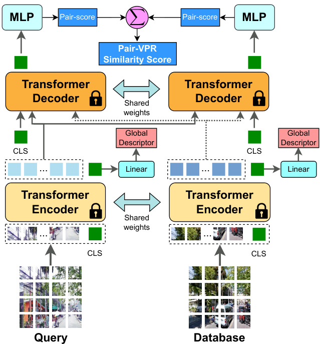
Fig. 2: During inference, we pass in pairs of (query, database) images and the network produces a score estimating whether or not the pair of images are from the same location or not, along with a global descriptor per image.
图 2: 在推理过程中,我们输入(query, database)图像对,网络会生成一个分数来估计这对图像是否来自同一位置,同时为每张图像生成一个全局描述符。
In the second stage, for each query, we copy the dense features by $N$ in order to create batches of (query, database $;_{j}$ ) pairs, where $j$ is the database index and there are $N$ pairs in total. Because our decoder is not symmetric (self-attention is only performed on the first image in a pair), we pass into the decoder batches of both (query, databasej) and (databasej, query) pairs and then sum their respective scores. The highestscoring pair is then considered the best match for the current query. Figure 2 shows our network during evaluation.
在第二阶段,对于每个查询(query),我们将密集特征复制$N$次以创建(query, database$;_{j}$)对的批次,其中$j$是数据库索引,总共有$N$对。由于我们的解码器是非对称的(自注意力机制仅作用于每对中的第一张图像),我们将(query, databasej)和(databasej, query)对同时输入解码器,然后对它们各自的分数求和。得分最高的对即被视为当前查询的最佳匹配。图2展示了评估阶段的网络结构。
IV. IMPLEMENTATION DETAILS
IV. 实现细节
A. Stage One Training
A. 第一阶段训练
We begin by pre-initializing the ViT encoder with weights from DINOv2 [28]. We found that leveraging the diverse pre-training policy used in DINOv2 improved performance over random initialization (please refer to ablation studies in Table II). We then freeze the first half of the encoder blocks (e.g., six blocks with ViT-B) and train the second half using Place-Aware Masked Image Modeling. We train in a Placeaware fashion and construct a dataloader such that a single item in a batch is a single place, where an item comprises a pair of images. We selected three existing large open source datasets for stage one training: SF-XL [14], GSV-Cities [7], and Google Landmarks v2 [15].
我们首先使用DINOv2 [28]的权重对ViT编码器进行预初始化。实验发现,相较于随机初始化,采用DINOv2的多样化预训练策略能提升模型性能(详见表II消融实验)。随后冻结编码器前半部分模块(例如ViT-B架构中的前六个模块),通过位置感知掩码图像建模(Place-Aware Masked Image Modeling)训练后半部分模块。采用位置感知训练方式构建数据加载器,确保每个批次中的单个条目对应一个地点,该条目由图像对组成。第一阶段训练选用了三个现有大型开源数据集:SF-XL [14]、GSV-Cities [7]和Google Landmarks v2 [15]。
SF-XL: We follow the procedure described in Ei gen Places [36] and divide the dataset into $M\times M$ meter-sized cells based on the UTM coordinates of all panoramic images in the dataset, generating a total of $C$ cells. Considering the $i$ -th cell $C_{i}$ , we follow the approach in Ei gen Places of computing the Singular Value Decomposition (SVD) from the UTM coordinates of all images in this cell, along with the mean UTM coordinate $\mu_{i}$ for this cell. We then select pairs of panoramic images randomly from each cell. Given cell $C_{i}$ , we begin by calculating a random focal point (e.g., a target UTM coordinate) that we want our pairs to observe, anchored to the first principle component of the cell denoted as $V_{0}^{i}$ . Our formula for calculating a focal point is given below:
SF-XL:我们遵循Ei gen Places [36]中描述的方法,根据数据集中所有全景图像的UTM坐标将其划分为$M\times M$米大小的单元,共生成$C$个单元。对于第$i$个单元$C_{i}$,我们采用Ei gen Places中的方法,计算该单元内所有图像UTM坐标的奇异值分解(SVD)以及该单元的平均UTM坐标$\mu_{i}$。随后从每个单元中随机选取全景图像对。给定单元$C_{i}$时,我们首先计算一个随机焦点(例如目标UTM坐标),该焦点需位于单元的第一主成分$V_{0}^{i}$上。焦点计算公式如下:
$$
f_{i}=\mu_{i}+D_{i}\times{\bf R}\left(V_{0}^{i},O_{i}\right),
$$
$$
f_{i}=\mu_{i}+D_{i}\times{\bf R}\left(V_{0}^{i},O_{i}\right),
$$
where $O_{i}$ is a random observation angle, and $D_{i}$ is a random focal length. At each iteration, we randomly sample observation angles $O_{i}$ between 0 and 360 degrees and apply this random rotation to the ei gen vector $V_{0}^{i}$ . We then randomly sample different focal lengths $D_{i}$ , sampling between 10 and 20 meters away from the mean coordinate $\mu_{i}$ . This approach differs from the method in Ei gen Places, which only utilized the 0 and 90 degree observation angles and a fixed focal length.
其中 $O_{i}$ 是随机观测角度,$D_{i}$ 是随机焦距。每次迭代时,我们在0到360度之间随机采样观测角度 $O_{i}$ 并将其应用于特征向量 $V_{0}^{i}$。接着在距平均坐标 $\mu_{i}$ 10至20米的范围内随机采样不同焦距 $D_{i}$。该方法与Ei gen Places仅使用0度和90度观测角度及固定焦距的方案不同。
Then given a focal point $f_{i}$ , we produce crops from two randomly sampled panoramic images within cell $C_{i}$ , such that the cropped views are focused on the target focal point - this ensures that our pair of images contains overlapping visual information, without requiring any manual curation of pairs. We can then calculate a viewing angle between a given panoramic image $j$ and a focal point using their respective UTM coordinates:
给定一个焦点 $f_{i}$,我们从单元 $C_{i}$ 中随机选取两张全景图像进行裁剪,确保裁剪后的视图聚焦于目标焦点——这种方法能保证图像对包含重叠的视觉信息,且无需人工筛选配对。接着,可通过全景图像 $j$ 与焦点的UTM坐标计算视角:
$$
\alpha_{j}=a r c t a n\left(\frac{e_{f}-e_{j}}{n_{f}-n_{j}}\right).
$$
$$
\alpha_{j}=a r c t a n\left(\frac{e_{f}-e_{j}}{n_{f}-n_{j}}\right).
$$
Given this viewing angle, we select a 512 by 512 pixel crop from a 3328 by 512 pixel panoramic image. However, pairs can be selected that are either too easy (small viewpoint difference), or too hard (too much viewpoint difference). Therefore, we calculate the difference in angles between our two sampled crops:
鉴于这一视角,我们从3328×512像素的全景图中选取512×512像素的裁剪区域。但所选图像对可能过于简单(视角差异过小)或过于困难(视角差异过大)。因此,我们计算了两个采样裁剪区域之间的角度差:
$$
\theta_{i}=\angle\alpha_{1}-\angle\alpha_{2}.
$$
$$
\theta_{i}=\angle\alpha_{1}-\angle\alpha_{2}.
$$
Then we check if $\theta_{i}$ is between a low and high threshold $3^{\circ}$ and $50^{\circ}$ . If not, we resample until we return a pair of crops within the required range.
然后检查 $\theta_{i}$ 是否介于 $3^{\circ}$ 和 $50^{\circ}$ 的高低阈值之间。若不符合条件,则重新采样直至返回符合要求范围内的裁剪对。
GSV-Cities: We randomly sample a pair of images from each place in the GSV-Cities dataset, excluding places with less than 4 images available.
GSV-Cities:我们从GSV-Cities数据集的每个地点随机抽取一对图像,排除可用图像少于4张的地点。
GLDv2: To improve the data diversity, we also added the Google Landmarks dataset [15]. We only use the cleaned subset of the dataset to avoid damaging the network’s ability to learn by providing ambiguous image pairs. Additionally, we also exclude any landmarks with less than 4 images. We consider a landmark as a proxy for a place and treat the dataset in the same format as SF-XL and GSV-Cities. In total, we are left with 72, 322 landmarks for training after cleaning and filtering.
GLDv2:为提高数据多样性,我们还加入了Google Landmarks数据集[15]。仅使用该数据集的清洗子集,以避免通过提供模糊图像对损害网络学习能力。同时排除图像少于4张的地标点,将每个地标视为地点的代理,并以与SF-XL和GSV-Cities相同的格式处理数据集。经过清洗过滤后,最终获得72,322个地标点用于训练。
Training Summary: We merge the three aforementioned datasets to produce a total of 266809 places per epoch, which are sampled from a set of 3.43 million panoramic images and 2.08 million egocentric images. We train using a mask ratio of 90 percent with a ViT-B sized decoder for 500 epochs with a learning rate of 2e-4 for a batch size of 512 places with AdamW and a cosine LR scheduler. We train using square images of size 224 pixels. By default, we use a ViT-B encoder with 4 register tokens, however, we note that our approach can also work with larger encoder sizes. Hyper parameters for larger encoders are kept the same except we use 1000 epochs.
训练总结:我们将上述三个数据集合并,每轮训练共生成266809个地点样本,这些样本来自343万张全景图像和208万张第一视角图像。训练采用90%的掩码比例,使用ViT-B尺寸的解码器进行500轮训练,学习率为2e-4,批量大小为512个地点,优化器为AdamW并采用余弦学习率调度器。训练使用224像素见方的图像。默认情况下,我们使用带有4个寄存器token的ViT-B编码器,但我们的方法同样适用于更大尺寸的编码器。更大编码器的超参数保持不变,仅将训练轮数调整为1000轮。
B. Stage Two Training
B. 第二阶段训练
We continue training our model using the GSV-Cities dataset [7] following the training recipe used in prior works such as MixVPR [20] and SALAD [37]. We train for 10 epochs using a linear LR scheduler with an initial LR of 8e-5, with a weight decay of 5e-2 and a batch size of 100 places. We also use square images of size 322, and freeze all encoder layers except the last six. Our global descriptor has only 512 dimensions and we set $w$ (the loss balance term) to 2. Hyper parameters were set using a grid search on the MSLSVal set. We use MSLS-Val as our validation dataset and take the checkpoint with the highest second-stage Recall $@1$ as the final trained model.
我们继续使用GSV-Cities数据集[7]训练模型,遵循MixVPR[20]和SALAD[37]等先前工作中采用的训练方案。训练共进行10个周期,采用初始学习率为8e-5的线性学习率调度器,权重衰减为5e-2,每批处理100个地点。输入图像统一调整为322×322像素正方形,并冻结除最后六层外的所有编码器层。全局描述符维度仅为512,损失平衡项$w$设为2。所有超参数均通过在MSLS-Val验证集上进行网格搜索确定。我们选用MSLS-Val作为验证数据集,并选取第二阶段Recall@1最高的检查点作为最终训练模型。
C. Evaluation
C. 评估
We evaluate our method on five commonly used benchmark VPR datasets, with a diverse set of environments. The datasets are: MSLS validation set [38], MSLS challenge set [38], Pittsburgh 30 k [39], Tokyo247 [40] and Nordland [41] (note that we use the split of Nordland from VPRBench [42], with 2760 query images). During the evaluation, we resize all images to $322\times322$ resolution. By default, Pair-VPR uses a ViT-B encoder and uses the top 100 candidates after global descriptor matching - we refer to this as the Speed configuration of Pair-VPR (Pair-VPR-s). We also provide a Performance version of Pair-VPR, which has a ViT-G encoder and uses the top 500 candidates during pair-classification (PairVPR-p). We evaluate using the standard Recall $\ @\mathrm{N}$ metric [3], [14] with $N\in{1,5,10}$ .
我们在五个常用的基准视觉位置识别(VPR)数据集上评估了我们的方法,这些数据集涵盖了多样化的环境。数据集包括:MSLS验证集[38]、MSLS挑战集[38]、Pittsburgh 30k[39]、Tokyo247[40]和Nordland[41](注:我们使用VPRBench[42]提供的Nordland划分,包含2760张查询图像)。评估过程中,所有图像均被调整为$322\times322$分辨率。默认情况下,Pair-VPR采用ViT-B编码器,并在全局描述符匹配后保留前100个候选——我们称之为Pair-VPR的速度配置(Pair-VPR-s)。我们还提供了Pair-VPR的性能版本,该版本采用ViT-G编码器,并在配对分类阶段保留前500个候选(PairVPR-p)。评估采用标准的Recall$\ @\mathrm{N}$指标[3][14],其中$N\in{1,5,10}$。
To compare Pair-VPR with existing techniques, we benchmark against five existing single-stage learnt VPR methods (CosPlace [14], MixVPR [20], Ei gen Places [36], BoQ [43] and SALAD [37]) and three existing two-stage VPR techniques (Patch-NetVLAD [9], R2Former [22] and SelaVPR [8]). We also include a baseline single-stage ViT VPR system we refer to as PaVPR (Place-aware VPR), which uses the same Stage One training as Pair-VPR except discards the pair contrastive training component during Stage Two and has a global descriptor with 512 dimensions.
为比较Pair-VPR与现有技术,我们选取了五种现有单阶段学习型VPR方法(CosPlace [14]、MixVPR [20]、EigenPlaces [36]、BoQ [43]和SALAD [37])以及三种现有两阶段VPR技术(Patch-NetVLAD [9]、R2Former [22]和SelaVPR [8])进行基准测试。同时引入一个单阶段ViT VPR基线系统PaVPR(Place-aware VPR),其第一阶段训练与Pair-VPR相同,但在第二阶段舍弃了配对对比训练组件,并采用512维全局描述符。
V. RESULTS AND DISCUSSION
V. 结果与讨论
A. Comparison to Recent VPR Methods
A. 与近期VPR方法的比较
We begin by comparing the performance of Pair-VPR against other State-Of-The-Art (SOTA) VPR methods on a range of benchmark datasets (Table I). Comparing our method, Pair-VPR-s, to the other methods we benchmark, we observe that Pair-VPR achieves the highest Recall $@1$ on all five datasets. We observe that our transformer-based re-ranking network is particularly adept at improving the Recall $@1$ over other works that also use a vision transformer backbone (SALAD [37], SelaVPR [8], and our $\scriptstyle{\mathrm{PaVPR}}$ baseline). Comparing against R2Former [22], a prior SOTA method that also used a re-ranking/pair-classifier transformer, we observe a significant jump in performance, especially on the Tokyo dataset.
我们首先将 Pair-VPR 与其他最先进的视觉位置识别 (VPR) 方法在多个基准数据集上的性能进行比较 (表1)。通过将我们的方法 Pair-VPR-s 与其他基准方法对比,可以观察到 Pair-VPR 在所有五个数据集上都取得了最高的 $@1$ 召回率。特别值得注意的是,基于 Transformer 的重排序网络在提升 $@1$ 召回率方面表现尤为突出,优于同样采用视觉 Transformer 骨干网络的其他工作 (SALAD [37]、SelaVPR [8] 以及我们的 $\scriptstyle{\mathrm{PaVPR}}$ 基线)。与同样采用 Transformer 重排序/配对分类器的先前 SOTA 方法 R2Former [22] 相比,我们的方法性能提升显著,尤其在 Tokyo 数据集上表现突出。
TABLE I: Quantitative results for VPR methods on benchmark datasets. Rows above and below the line denote single-stage and two-stage VPR methods respectively. Underlined numbers denote the second best in a column.
表 1: 基准数据集上VPR方法的定量结果。横线上方和下方的行分别表示单阶段和两阶段VPR方法。带下划线的数字表示该列中第二好的结果。
| Method | Enc.Size | MSLS-Val R@1 | MSLS-Val R@5 | MSLS-Val R@10 | MSLS-Challenge R@1 | MSLS-Challenge R@5 | MSLS-Challenge R@10 | Pitts30k R@1 | Pitts30k R@5 | Pitts30k R@10 | Tokyo24/7 R@1 | Tokyo24/7 R@5 | Tokyo24/7 R@10 | Nordland R@1 | Nordland R@5 | Nordland R@10 |
|---|---|---|---|---|---|---|---|---|---|---|---|---|---|---|---|---|
| CosPlace [14] | ResNet-50 | 87.4 | 94.1 | 94.9 | 67.0 | 77.9 | 80.7 | 90.9 | 95.7 | 96.7 | 87.3 | 94.0 | 95.6 | 55.3 | 71.5 | 77.5 |
| MixVPR [20] | ResNet-50 | 88.0 | 92.7 | 94.6 | 64.0 | 75.9 | 80.6 | 91.5 | 95.5 | 96.3 | 85.1 | 91.7 | 94.3 | 58.4 | 74.6 | 80.0 |
| EigenPlaces [36] | ResNet-50 | 89.1 | 93.8 | 95.0 | 67.4 | 77.1 | 81.7 | 92.5 | 96.8 | 97.6 | 92.4 | 96.2 | 97.1 | 54.4 | 68.8 | 74.1 |
| BoQ [43] | ResNet-50 | 91.2 | 95.3 | 96.1 | 72.8 | 83.1 | 86.3 | 92.4 | 96.5 | 97.4 | 90.5 | 95.2 | 96.5 | 70.7 | 84.0 | 87.5 |
| SALAD [37] | ViT-B | 92.2 | 96.4 | 97.0 | 75.0 | 88.8 | 91.3 | 92.4 | 96.3 | 97.4 | 95.2 | 97.1 | 98.1 | 76.0 | 89.2 | 92.0 |
| PaVPRbaseline | ViT-B | 89.5 | 94.5 | 95.8 | 67.8 | 80.5 | 83.8 | 90.4 | 95.4 | 96.8 | 86.4 | 94.6 | 95.6 | 57.7 | 75.5 | 80.8 |
| Patch-NetVLAD-s [9] | VGG-16 | 77.3 | 84.2 | 86.5 | 35.8 | 50.1 | 55.3 | 87.1 | 93.9 | 95.4 | 67.6 | 74.6 | 77.8 | 24.8 | 29.2 | 30.7 |
| R2Former [22] | ViT-S | 89.7 | 95.0 | 96.2 | 73.0 | 85.9 | 88.8 | 91.1 | 95.2 | 96.3 | 88.6 | 91.4 | 91.7 | |||
| SelaVPR [8] | ViT-L | 90.8 | 96.4 | 97.2 | 73.5 | 87.5 | 90.6 | 92.8 | 96.8 | 97.7 | 94.0 | 96.8 | 97.5 | 66.2 | 79.8 | 84.1 |
| Pair-VPR-s (Ours) | ViT-B | 93.7 | 97.2 | 97.3 | 79.0 | 86.9 | 88.3 | 94.7 | 97.2 | 97.8 | 98.1 | 98.4 | 98.7 | 84.2 | 90.9 | 91.6 |
| Pair-VPR-p (Ours) | ViT-G | 95.4 | 97.3 | 97.7 | 81.7 | 90.2 | 91.3 | 95.4 | 97.5 | 98.0 | 100 | 100 | 100 | 91.0 | 95.2 | 95.7 |
TABLE II: Stage One Training Ablation Study for VPR. Bold denotes the standard configurations of Pair-VPR.
表 II: VPR 第一阶段训练消融研究。加粗表示 Pair-VPR 的标准配置。
| 消融方案 | 编码器尺寸 | 初始化 | MSLS-Val R@1 | MSLS-Val R@5 | MSLS-Val R@10 | Pitts30k R@1 | Pitts30k R@5 | Pitts30k R@10 | Tokyo24/7 R@1 | Tokyo24/7 R@5 | Tokyo24/7 R@10 | Nordland R@1 | Nordland R@5 | Nordland R@10 |
|---|---|---|---|---|---|---|---|---|---|---|---|---|---|---|
| 无第一阶段训练 | ViT-B | DINOv2 | 78.2 | 95.4 | 96.1 | 89.3 | 95.3 | 96.5 | 92.1 | 97.1 | 97.8 | 54.5 | 74.6 | 78.6 |
| 无配对训练 | ViT-B | DINOv2 | 91.2 | 95.0 | 95.7 | 91.8 | 95.8 | 96.8 | 93.0 | 94.9 | 95.6 | 67.3 | 76.4 | 78.5 |
| 解冻所有编码块 | ViT-B | DINOv2 | 91.9 | 96.0 | 96.8 | 93.1 | 96.5 | 97.2 | 94.3 | 95.9 | 96.2 | 78.7 | 86.6 | 88.3 |
| 从头训练 | ViT-B | Random | 88.4 | 91.5 | 91.8 | 92.8 | 95.8 | 96.4 | 83.2 | 85.4 | 86.4 | 42.7 | 45.9 | 46.3 |
| Pair-VPR-s (Top100-B) | ViT-B | DINOv2 | 93.7 | 97.2 | 97.3 | 94.7 | 97.2 | 97.8 | 98.1 | 98.4 | 98.7 | 84.2 | 90.9 | 91.6 |
| Pair-VPR (Top100-L) | ViT-L | DINOv2 | 94.5 | 97.0 | 97.4 | 94.0 | 97.0 | 97.8 | 96.8 | 96.8 | 96.8 | 86.6 | 91.2 | 91.5 |
| Pair-VPR (Top100-G) | ViT-G | DINOv2 | 95.1 | 97.2 | 97.6 | 95.4 | 97.5 | 97.9 | 98.4 | 98.4 | 98.4 | 85.8 | 89.1 | 89.4 |
| Pair-VPR-p (Top500-G) | ViT-G | DINOv2 | 95.4 | 97.3 | 97.7 | 95.4 | 97.5 | 98.0 | 100 | 100 | 100 | 91.0 | 95.2 | 95.7 |
When we scale up our method to use larger encoder sizes and more top candidates, we observe that Pair-VPR-p provides a large performance increase over Pair-VPR-s and achieves the highest recall across all Recall $\ @\mathrm{N}$ values compared to prior works. We especially highlight the results on Tokyo24/7, where we have achieved a Recall $@1$ of $100%$ .
当我们将方法扩展到使用更大的编码器尺寸和更多候选对象时,观察到Pair-VPR-p相比Pair-VPR-s带来了显著的性能提升,并且在所有Recall $\ @\mathrm{N}$ 值上均超越了先前工作,达到最高召回率。特别值得注意的是在Tokyo24/7数据集上的结果,我们实现了 $100%$ 的Recall $@1$。
We also include results on Pair-VPR-s when the number of top candidates that are re-ranked by Pair-VPR are varied (Figure 3). The graph shows that a lower number of top candidates can still achieve good VPR performance, especially on the MSLS-Val and Pitts30k datasets. This is because the PairVPR global descriptor has good performance on these datasets. Tokyo24/7 exhibits a similar trend, except that a larger number of top candidates allows the Pair-VPR re-ranking to achieve very high recalls. We observe that increasing the number of top candidates has significant benefits on the Nordland dataset. The Nordland split from VPRBench is very challenging, with a lot of perceptual aliasing and a small localization error tolerance; therefore, a larger number of top candidates is necessary on this dataset.
我们还展示了当Pair-VPR重新排序的候选数量变化时,Pair-VPR-s的结果(图3)。图表显示,较少的候选数量仍能实现良好的VPR性能,尤其是在MSLS-Val和Pitts30k数据集上。这是因为PairVPR全局描述符在这些数据集上表现良好。Tokyo24/7也呈现类似趋势,只是更多的候选数量能让Pair-VPR重排序达到非常高的召回率。我们观察到,增加候选数量对Nordland数据集有明显益处。VPRBench中的Nordland划分极具挑战性,存在大量感知混淆且定位误差容忍度较小,因此该数据集需要更多候选数量。
B. Pre-training Ablation Study
B. 预训练消融研究
To understand which aspects of our training strategy are essential for the performance of Pair-VPR, we conducted an ablation study over different variations of stage one training (Table II). In the first row, we show the results when we do not perform stage one training at all, with the decoder in stage two initialized using random weights. We observed that pre-training the decoder network via stage one training is essential for achieving effective VPR performance - since the pair-classification task is non-trivial, the place-aware Siamese mask image modeling task provides an initial set of weights that are already tuned for comparing features between two images.
为了探究训练策略中哪些要素对Pair-VPR性能至关重要,我们对第一阶段训练的不同变体进行了消融实验(表II)。首行展示了完全不进行第一阶段训练时的情况,此时第二阶段解码器采用随机初始化权重。实验表明,通过第一阶段训练对解码器网络进行预训练是实现有效VPR性能的关键——由于图像对分类任务本身具有挑战性,基于位置感知的孪生掩码图像建模任务能提供一组已针对双图像特征比对优化的初始权重。

Fig. 3: Recall $@1$ as the number of re-ranked candidates is increased for Pair-VPR-s.
图 3: Pair-VPR-s 在不同重排序候选数量下的召回率 (Recall) $@1$
In the second row of Table II, we investigated the importance of place-aware sampling by removing the place sampling during stage one training, and instead used strong augmentation to generate the second unmasked image. We observed a consistent drop in recall, even though the total collection of training images remains identical.
在表 II 的第二行中,我们通过移除第一阶段训练中的地点感知采样 (place-aware sampling) ,转而使用强数据增强生成第二张未掩码图像,研究了该方法的重要性。尽管训练图像的总集合保持不变,但我们观察到召回率持续下降。
In row three, we experimented with unfreezing all blocks in our DINOv2-initialized ViT encoder. We found that allowing the entire network to be trained reduced the VPR performance, and we hypothesize that this is because the DINOv2 network was originally trained on a larger and more diverse dataset than ours, and maintaining the low level (e.g., color) learnt features from a more diverse dataset improves performance.
在第三行实验中,我们尝试解冻DINOv2初始化的ViT编码器中所有模块。发现允许整个网络参与训练会降低视觉位置识别(VPR)性能,推测这是因为DINOv2网络原始训练数据集比我们使用的规模更大、多样性更强,保留从更丰富数据集中学习到的底层特征(如色彩)有助于提升性能。
TABLE III: Performance of the Pair-VPR Global Descriptor.
表 III: Pair-VPR全局描述符性能
| 方法 | MSLS-Val | Pitts30k | Tokyo24/7 | ||||||
|---|---|---|---|---|---|---|---|---|---|
| R@1 | R@100 | R@500 | R@1 | R@100 | R@500 | R@1 | R@100 | R@500 | |
| Pair-VPR-s (Global) | 86.4 | 97.8 | 98.5 | 89.3 | 99.0 | 99.8 | 85.1 | 99.1 | 99.7 |
| Pair-VPR-s (Refine) | 93.7 | 97.8 | 97.8 | 94.7 | 99.0 | 99.0 | 98.1 | 99.1 | 99.1 |
| Pair-VPR-p (Global) | 86.6 | 98.4 | 98.8 | 90.2 | 99.1 | 99.6 | 77.8 | 99.1 | 100 |
| Pair-VPR-p (Refine) | 95.4 | 98.5 | 98.8 | 95.4 | 99.3 | 99.6 | 100 | 100 | 100 |
In the fourth row we instead initialized the ViT encoder with random weights and performed stage one training from scratch. We found that the VPR performance is still maintained well on urban datasets, but reduces significantly on non-urban datasets, such as Nordland. This is likely due to the urban bias in common VPR pre-training datasets.
在第四行中,我们改用随机权重初始化ViT编码器,并从零开始进行第一阶段训练。我们发现VPR性能在城市数据集上仍保持良好,但在非城市数据集(如Nordland)上显著下降。这可能是由于常见VPR预训练数据集中存在城市偏见。
In the bottom four rows, we compared different configurations of Pair-VPR. We observed that the performance of PairVPR improves as we increase the encoder size. We further observed that increasing the number of top candidates passed to the pair classification component improves the recall, as it alleviates the performance limitation imposed by the global descriptor’s effectiveness.
在底部四行中,我们比较了Pair-VPR的不同配置。我们观察到,随着编码器尺寸的增加,PairVPR的性能有所提升。此外,我们还发现,增加传递给配对分类组件的候选数量可以提高召回率,因为这缓解了全局描述符有效性带来的性能限制。
C. Performance of the Pair-VPR Global Descriptor
C. Pair-VPR全局描述符的性能
In Table III, we analyze the performance of the Pair-VPR global descriptor. The performance of the second stage refinement is always limited by the recall of the global descriptor at the chosen number of top candidates, therefore we display Recall $\ @\mathrm{N}$ values for $N\in{1,100,50\mathrm{{C}}}$ . The global descriptor is always 512 dimensions, allowing for computationally efficient database searching while also having a Recall $@1$ comparable to existing global descriptor VPR methods. We also note that our global descriptor is a lot smaller than the single-stage VPR methods in Table I, e.g., CosPlace, MixVPR and SALAD have 2048, 4096 and 8448 dimensions respectively.
在表 III 中,我们分析了 Pair-VPR 全局描述符的性能。第二阶段精修的性能始终受限于所选候选数量下全局描述符的召回率,因此我们展示了 $N\in{1,100,50\mathrm{{C}}}$ 时的 Recall $\ @\mathrm{N}$ 值。该全局描述符始终保持 512 维,既能实现高效计算的数据库搜索,又具备与现有全局描述符 VPR 方法相当的 Recall $@1$ 性能。我们还注意到,相较于表 I 中的单阶段 VPR 方法(如 CosPlace、MixVPR 和 SALAD 分别具有 2048、4096 和 8448 维),我们的全局描述符维度显著更低。
When we shift to using larger encoder sizes, we always maintain the same global descriptor by increasing the projection ratio from the class token. For a ViT-G encoder, the class token has 1530 dimensions and we project down to 512 dimensions using a linear layer. We do this in order to keep the computational cost of descriptor matching the same. We find that the ViT-G global descriptor performs similar to the ViT-B descriptor, except on Tokyo24/7. It is possible that the large projection ratio is not ideal for VPR, therefore future work should investigate experimenting with larger global descriptor sizes, albeit at an increased compute requirement.
当我们转向使用更大的编码器尺寸时,始终通过增加类别token (class token) 的投影比例来保持相同的全局描述符。对于ViT-G编码器,类别token具有1530维,我们使用线性层将其投影至512维。此举是为了保持描述符匹配的计算成本不变。我们发现ViT-G全局描述符的表现与ViT-B描述符相近,但在Tokyo24/7数据集上例外。较大的投影比例可能不适用于视觉位置识别 (VPR) ,因此未来工作应探索使用更大全局描述符尺寸的实验,尽管这会增加计算需求。
TABLE IV: Compute Analysis of two-stage methods.
表 IV: 两阶段方法的计算分析
| 方法 | 编码 (ms/查询) | 匹配 (ms/查询) | 优化 (ms/对) | 存储 (mB/图像) |
|---|---|---|---|---|
| Patch-NetVLAD-s | 12.51 | 0.17 | 0.94 | 1.83 |
| Patch-NetVLAD-p | 211.0 | 0.26 | 32.32 | 45.22 |
| R2Former | 7.11 | 0.33 | 0.74 | 0.25 |
| SelaVPR | 9.71 | 0.08 | 0.91 | 0.46 |
| Pair-VPR-s (ViT-B) | 7.31 | 0.13 | 7.18 | 1.55 |
| Pair-VPR-p (ViT-G) | 33.17 | 0.13 | 7.31 | 3.10 |

Fig. 4: Qualitative results on the benchmark datasets, showing the performance of the computationally cheapest version of Pair-VPR (Pair-VPR-s). We provide three success examples and two failure cases per dataset.
图 4: 基准数据集上的定性结果,展示了计算成本最低的 Pair-VPR (Pair-VPR-s) 版本性能。我们为每个数据集提供了三个成功案例和两个失败案例。
D. Compute Analysis
D. 计算分析
In this subsection we discuss the computational requirements of Pair-VPR and compare against other two-stage VPR methods on MSLS-Val, using the same compute platform (a single GPU), as shown in Table IV. It can be seen that PairVPR-s is fast at encoding and matching, taking 7 milliseconds per query image to encode and only $0.13~\mathrm{ms}{}/\$ query to match against the entire database using 512 dimensional descriptors. Our second stage refinement is slower than SelaVPR and R2Former but much faster than Patch-NetVLAD-p, and requires 0.7 seconds per query with 100 top candidates. Comparing the ViT-B to ViT-G encoder sizes of Pair-VPR, only the encoding time and storage requirement increases, since we maintain the same global descriptor size and the same decoder network size. The storage requirements of Pair-VPR are primarily from the dense features required for refinement and Pair-VPR-s features are comparable in size to PatchNetVLAD-s and SelaVPR.
在本小节中,我们讨论Pair-VPR的计算需求,并在MSLS-Val数据集上与其他两阶段VPR方法进行比较(使用相同的计算平台:单块GPU),如表IV所示。可以看出,PairVPR-s在编码和匹配阶段速度极快,每张查询图像仅需7毫秒完成编码,使用512维描述符时全局数据库匹配仅需$0.13~\mathrm{ms}{}/$查询。我们的第二阶段精炼速度虽慢于SelaVPR和R2Former,但远快于Patch-NetVLAD-p,在保留100个候选时每查询耗时0.7秒。对比Pair-VPR的ViT-B与ViT-G编码器规模,仅编码时间和存储需求会随模型增大而增加,因为我们保持相同的全局描述符维度和解码器网络规模。Pair-VPR的存储需求主要来自精炼所需的密集特征,其Pair-VPR-s特征大小与PatchNetVLAD-s和SelaVPR相当。
E. Qualitative Analysis
E. 定性分析
In Figure 4, we provide qualitative results for Pair-VPR-s, including success and failure examples. The success examples show that Pair-VPR can successfully localize even in challenging situations such as at nighttime, under viewpoint shifts, or seasonal changes like summer to winter. The failure cases provide insights about challenging situations for VPR systems. For example, on the MSLS-Val dataset we show a failure due to heavy occlusion, and a second failure due to an upside down image in the dataset. In the case of the occluded image (due to a bus), these situations merit the addition of sequential VPR methods (e.g., [44]) to include adjacent image frames that may not be occluded. Concerning the failure examples on the Tokyo24/7 dataset, nighttime conditions are a common failure mode in VPR systems due to the lack of visible features at nighttime - although we note that these failure cases are solved by the more powerful Pair-VPR-p system, which has significantly more parameters in its ViT-G encoder.
在图4中,我们展示了Pair-VPR-s的定性结果,包括成功和失败案例。成功案例表明,即使在夜间、视角变化或夏冬季节变化等挑战性场景下,Pair-VPR仍能准确定位。失败案例则揭示了VPR系统面临的典型挑战:例如在MSLS-Val数据集中,一个失败源于严重遮挡(公交车),另一个由数据集中倒置图像导致。针对遮挡情况,建议结合序列化VPR方法(如[44])引入相邻未遮挡图像帧。对于Tokyo24/7数据集的夜间失败案例,这反映了VPR系统普遍存在的夜间特征缺失问题——值得注意的是,参数量更大的ViT-G编码器版本Pair-VPR-p成功解决了这些案例。
VI. CONCLUSION
VI. 结论
In summary, we present Pair-VPR, a novel two-stage VPR method that relies upon a mask image modeling pre-training strategy to maximize performance. Pair-VPR combines a small 512 dimensional global descriptor for rapid database searching along with a slower second stage that only searches a set of potential database matches. We observed that Pair-VPR achieved the highest Recall $@1$ score on all datasets we tested on, comparing against recent state-of-the-art methods in VPR literature - while only requiring an encoder and decoder of 86 million parameters each. As the encoder size is scaled up to ViT-L (307M) and ViT-G (1.1B), our training recipe allows for continuing performance improvements as the network size grows. Given the high recalls attained by Pair-VPR, we believe it prudent to investigate converting this method from a VPR technique to a loop closure module in a full SLAM system. In the future, we aim to examine the effectiveness of Pair-VPR at performing loop closures in SLAM.
总之,我们提出了Pair-VPR这一新颖的两阶段视觉位置识别(VPR)方法,该方法采用掩码图像建模预训练策略以实现最佳性能。Pair-VPR结合了512维小型全局描述符用于快速数据库检索,以及仅搜索潜在匹配集的较慢第二阶段。实验表明,在对比近期VPR领域最先进方法时,Pair-VPR在所有测试数据集上均取得了最高的Recall $@1$分数,而仅需各8600万参数的编码器和解码器。当编码器规模扩展至ViT-L(3.07亿)和ViT-G(11亿)时,我们的训练方案能持续提升网络性能。鉴于Pair-VPR实现的高召回率,我们认为将其从VPR技术转化为完整SLAM系统中的回环检测模块是值得研究的。未来我们将探索Pair-VPR在SLAM中执行回环检测的有效性。