V-Net: Fully Convolutional Neural Networks for Volumetric Medical Image Segmentation

V-Net: 用于三维医学图像分割的全卷积神经网络

Abstract. Convolutional Neural Networks (CNNs) have been recently employed to solve problems from both the computer vision and medical image analysis fields. Despite their popularity, most approaches are only able to process 2D images while most medical data used in clinical practice consists of 3D volumes. In this work we propose an approach to 3D image segmentation based on a volumetric, fully convolutional, neural network. Our CNN is trained end-to-end on MRI volumes depicting prostate, and learns to predict segmentation for the whole volume at once. We introduce a novel objective function, that we optimise during training, based on Dice coefficient. In this way we can deal with situations where there is a strong imbalance between the number of foreground and background voxels. To cope with the limited number of annotated volumes available for training, we augment the data applying random non-linear transformations and histogram matching. We show in our experimental evaluation that our approach achieves good performances on challenging test data while requiring only a fraction of the processing time needed by other previous methods.

摘要。卷积神经网络 (CNN) 最近被用于解决计算机视觉和医学图像分析领域的问题。尽管很受欢迎，但大多数方法只能处理 2D 图像，而临床实践中使用的大多数医学数据由 3D 体积组成。在这项工作中，我们提出了一种基于体积全卷积神经网络的 3D 图像分割方法。我们的 CNN 在描绘前列腺的 MRI 体积上进行端到端训练，并学会一次性预测整个体积的分割。我们引入了一种新的目标函数，在训练期间对其进行优化，该函数基于 Dice 系数。通过这种方式，我们可以处理前景和背景体素数量严重不平衡的情况。为了应对可用于训练的带注释体积数量有限的问题，我们通过应用随机非线性变换和直方图匹配来增强数据。我们在实验评估中表明，我们的方法在具有挑战性的测试数据上取得了良好的性能，同时只需要其他先前方法所需处理时间的一小部分。

1 Introduction and Related Work

1 引言与相关工作

Recent research in computer vision and pattern recognition has highlighted the capabilities of Convolutional Neural Networks (CNNs) to solve challenging tasks such as classification, segmentation and object detection, achieving state-of-theart performances. This success has been attributed to the ability of CNNs to learn a hierarchical representation of raw input data, without relying on handcrafted features. As the inputs are processed through the network layers, the level of abstraction of the resulting features increases. Shallower layers grasp local information while deeper layers use filters whose receptive fields are much broader that therefore capture global information [19].

计算机视觉与模式识别领域的最新研究凸显了卷积神经网络(CNN)在分类、分割和物体检测等复杂任务中的卓越能力，这些网络无需依赖人工特征工程即可实现最先进的性能表现。CNN的成功归因于其能够从原始输入数据中学习层次化表征的特性：随着数据在网络层级间传递，生成特征的抽象程度会逐层提升——浅层网络捕捉局部信息，而深层网络则通过具有更大感受野的滤波器来获取全局信息[19]。

Segmentation is a highly relevant task in medical image analysis. Automatic delineation of organs and structures of interest is often necessary to perform tasks such as visual augmentation [10], computer assisted diagnosis [12], interventions [20] and extraction of quantitative indices from images [1]. In particular, since diagnostic and interventional imagery often consists of 3D images, being able to perform volumetric segmentation s by taking into account the whole volume content at once, has a particular relevance. In this work, we aim to segment prostate MRI volumes. This is a challenging task due to the wide range of appearance the prostate can assume in different scans due to deformations and variations of the intensity distribution. Moreover, MRI volumes are often affected by artefacts and distortions due to field in homogeneity. Prostate segmentation is nevertheless an important task having clinical relevance both during diagnosis, where the volume of the prostate needs to be assessed [13], and during treatment planning, where the estimate of the anatomical boundary needs to be accurate [4,20].

分割是医学图像分析中一项高度相关的任务。自动勾画目标器官和结构通常对执行视觉增强 [10]、计算机辅助诊断 [12]、介入治疗 [20] 以及从图像中提取定量指标 [1] 等任务至关重要。特别是由于诊断和介入影像通常由3D图像构成，能够通过一次性考虑整个体积内容进行体积分割具有特殊意义。

在本研究中，我们的目标是分割前列腺MRI体积图像。这是一项具有挑战性的任务，因为前列腺在不同扫描中可能因形变和强度分布变化而呈现广泛的外观差异。此外，MRI体积图像常因磁场不均匀性而产生伪影和畸变。然而，前列腺分割仍是一项重要的临床相关任务：在诊断阶段需要评估前列腺体积 [13]，在治疗计划阶段则需精确估计解剖边界 [4,20]。

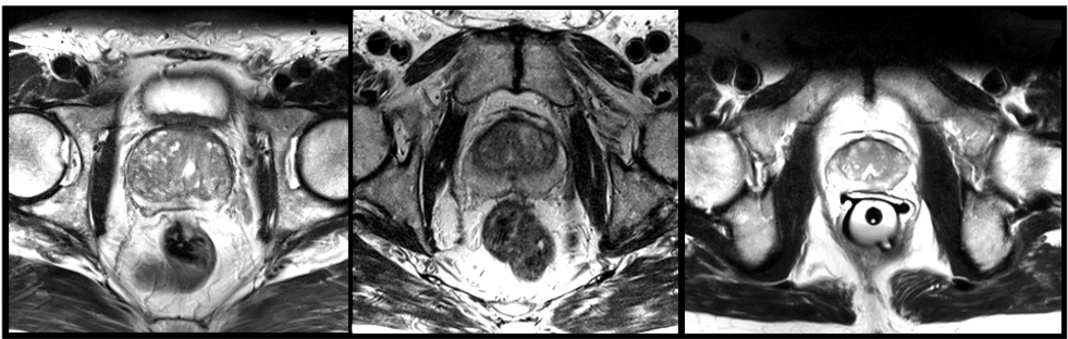
Fig. 1. Slices from MRI volumes depicting prostate. This data is part of the PROMISE 2012 challenge dataset [7].

图 1: 显示前列腺的 MRI 体积切片。该数据是 PROMISE 2012 挑战赛数据集的一部分 [7]。

CNNs have been recently used for medical image segmentation. Early approaches obtain anatomy delineation in images or volumes by performing patchwise image classification. Such segmentation s are obtained by only considering local context and therefore are prone to failure, especially in challenging modalities such as ultrasound, where a high number of mis-classified voxel are to be expected. Post-processing approaches such as connected components analysis normally yield no improvement and therefore, more recent works, propose to use the network predictions in combination with Markov random fields [6], voting strategies [9] or more traditional approaches such as level-sets [2]. Patch-wise approaches also suffer from efficiency issues. When densely extracted patches are processed in a CNN, a high number of computations is redundant and therefore the total algorithm runtime is high. In this case, more efficient computational schemes can be adopted.

CNN最近被用于医学图像分割。早期方法通过逐块图像分类来获取图像或体积中的解剖结构轮廓。这种分割方法仅考虑局部上下文，因此容易失败，尤其在具有挑战性的模态(如超声)中，预计会出现大量错误分类的体素。传统后处理方法(如连通域分析)通常无法改善结果，因此近期研究提出将网络预测与马尔可夫随机场[6]、投票策略[9]或更传统的方法(如水平集[2])结合使用。逐块方法还存在效率问题。当CNN处理密集提取的图像块时，大量计算是冗余的，导致算法总运行时间较长。这种情况下可采用更高效的计算方案。

Fully convolutional network trained end-to-end were so far applied only to 2D images both in computer vision [11,8] and microscopy image analysis [14]. These models, which served as an inspiration for our work, employed different network architectures and were trained to predict a segmentation mask, delineating the structures of interest, for the whole image. In [11] a pre-trained VGG network architecture [15] was used in conjunction with its mirrored, de-convolutional, equivalent to segment RGB images by leveraging the descriptive power of the features extracted by the innermost layer. In [8] three fully convolutional deep neural networks, pre-trained on a classification task, were refined to produce segmentation s while in [14] a brand new CNN model, especially tailored to tackle biomedical image analysis problems in 2D, was proposed.

全卷积网络 (fully convolutional network) 的端到端训练此前仅应用于计算机视觉 [11,8] 和显微图像分析 [14] 中的二维图像。这些模型为我们的工作提供了灵感，它们采用不同的网络架构，并被训练用于预测整张图像的分割掩模 (segmentation mask)，从而勾勒出目标结构。在 [11] 中，预训练的 VGG 网络架构 [15] 与其镜像的反卷积 (de-convolutional) 等效结构相结合，通过利用最内层提取的特征描述能力来分割 RGB 图像。在 [8] 中，三个在分类任务上预训练的全卷积深度神经网络经过微调以生成分割结果，而在 [14] 中则提出了一种专为解决二维生物医学图像分析问题而量身定制的新型 CNN 模型。

In this work we present our approach to medical image segmentation that leverages the power of a fully convolutional neural networks, trained end-to-end, to process MRI volumes. Differently from other recent approaches we refrain from processing the input volumes slice-wise and we propose to use volumetric convolutions instead. We propose a novel objective function based on Dice coefficient maxim is ation, that we optimise during training. We demonstrate fast and accurate results on prostate MRI test volumes and we provide direct comparison with other methods which were evaluated on the same test data 4.

在本工作中，我们提出了一种医学图像分割方法，该方法利用端到端训练的全卷积神经网络(full convolutional neural networks)处理MRI体积数据。与近期其他方法不同，我们避免对输入体积进行切片式处理，转而提出使用三维卷积(volumetric convolutions)。我们提出了一种基于Dice系数最大化(Dice coefficient maximisation)的新型目标函数，并在训练过程中进行优化。我们在前列腺MRI测试数据上展示了快速准确的分割结果，并与同组测试数据评估的其他方法进行了直接对比[4]。

2 Method

2 方法

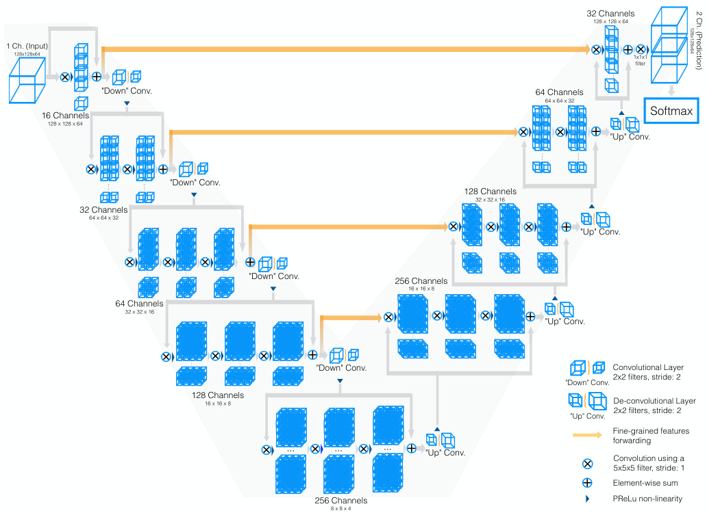
Fig. 2. Schematic representation of our network architecture. Our custom implementation of Caffe [5] processes 3D data by performing volumetric convolutions. Best viewed in electronic format.

图 2: 我们的网络架构示意图。我们基于Caffe [5]的定制实现通过执行体积卷积来处理3D数据。建议以电子格式查看最佳效果。

In Figure 2 we provide a schematic representation of our convolutional neural network. We perform convolutions aiming to both extract features from the data and, at the end of each stage, to reduce its resolution by using appropriate stride. The left part of the network consists of a compression path, while the right part decompresses the signal until its original size is reached. Convolutions are all applied with appropriate padding.

图 2: 我们展示了卷积神经网络 (Convolutional Neural Network) 的示意图。我们执行卷积操作的目的是从数据中提取特征，并在每个阶段结束时通过适当的步长 (stride) 降低分辨率。网络左侧由压缩路径组成，右侧则将信号解压缩直至恢复原始尺寸。所有卷积操作均采用适当的填充 (padding) 处理。

The left side of the network is divided in different stages that operate at different resolutions. Each stage comprises one to three convolutional layers. Similarly to the approach presented in [3], we formulate each stage such that it learns a residual function: the input of each stage is (a) used in the convolutional layers and processed through the non-linear i ties and (b) added to the output of the last convolutional layer of that stage in order to enable learning a residual function. As confirmed by our empirical observations, this architecture ensures convergence in a fraction of the time required by a similar network that does not learn residual functions.

网络的左侧被划分为多个在不同分辨率下运行的阶段。每个阶段包含一至三个卷积层。与[3]中提出的方法类似，我们将每个阶段设计为学习残差函数：每个阶段的输入 (a) 被用于卷积层并通过非线性处理，(b) 被添加到该阶段最后一个卷积层的输出中，以实现残差函数的学习。我们的实证观察证实，这种架构确保了在比不学习残差函数的类似网络所需时间更短的情况下实现收敛。

The convolutions performed in each stage use volumetric kernels having size $5\times5\times5$ voxels. As the data proceeds through different stages along the compression path, its resolution is reduced. This is performed through convolution with $2\times2\times2$ voxels wide kernels applied with stride 2 (Figure 3). Since the second operation extracts features by considering only non overlapping $2\times2\times2$ volume patches, the size of the resulting feature maps is halved. This strategy serves a similar purpose as pooling layers that, motivated by [16] and other works discouraging the use of max-pooling operations in CNNs, have been replaced in our approach by convolutional ones. Moreover, since the number of feature channels doubles at each stage of the compression path of the V-Net, and due to the formulation of the model as a residual network, we resort to these convolution operations to double the number of feature maps as we reduce their resolution. PReLu non linear i ties are applied throughout the network.

每个阶段执行的卷积运算使用大小为 $5\times5\times5$ 体素的体积核。随着数据沿压缩路径通过不同阶段，其分辨率会降低。这是通过应用步长为2的 $2\times2\times2$ 体素宽核的卷积来实现的 (图 3)。由于第二个操作仅考虑不重叠的 $2\times2\times2$ 体积块提取特征，因此生成的特征图尺寸会减半。该策略的目的类似于池化层，但受 [16] 等研究的启发（这些研究不鼓励在CNN中使用最大池化操作），我们的方法中已用卷积操作替代了池化层。此外，由于V-Net压缩路径每个阶段的特征通道数会翻倍，且模型采用残差网络结构，我们在降低分辨率的同时通过这些卷积操作将特征图数量翻倍。整个网络中均采用PReLU非线性激活函数。

Replacing pooling operations with convolutional ones results also to networks that, depending on the specific implementation, can have a smaller memory footprint during training, due to the fact that no switches mapping the output of pooling layers back to their inputs are needed for back-propagation, and that can be better understood and analysed [19] by applying only de-convolutions instead of un-pooling operations.

用卷积操作替代池化操作还能带来以下优势：根据具体实现方式，这类网络在训练时可能占用更少内存。这是因为反向传播时无需维护池化层输出到输入的映射开关，同时仅需使用反卷积（de-convolutions）而非逆池化（un-pooling）操作，使得网络更易于理解和分析 [19]。

Down sampling allows us to reduce the size of the signal presented as input and to increase the receptive field of the features being computed in subsequent network layers. Each of the stages of the left part of the network, computes a number of features which is two times higher than the one of the previous layer.

下采样 (down sampling) 可以减小输入信号的尺寸，同时增大后续网络层所计算特征的感受野。网络左侧的每个阶段计算的特征数量都是前一层的两倍。

The right portion of the network extracts features and expands the spatial support of the lower resolution feature maps in order to gather and assemble the necessary information to output a two channel volumetric segmentation. The two features maps computed by the very last convolutional layer, having $1\times1\times1$ kernel size and producing outputs of the same size as the input volume, are converted to probabilistic segmentation s of the foreground and background regions by applying soft-max voxelwise. After each stage of the right portion of the CNN, a de-convolution operation is employed in order increase the size of the inputs (Figure 3) followed by one to three convolutional layers involving half the number of $5\times5\times5$ kernels employed in the previous layer. Similar to the left part of the network, also in this case we resort to learn residual functions in the convolutional stages.

网络右侧部分提取特征并扩展低分辨率特征图的空间支持范围，以收集和整合必要信息，最终输出双通道体积分割结果。最后一层卷积层生成的两个特征图（采用$1\times1\times1$核尺寸，输出与输入体积尺寸相同）通过逐体素soft-max运算转换为前景与背景区域的概率分割图。在CNN右侧每个阶段处理后，会执行反卷积操作以扩大输入尺寸（图3），随后接入1至3个卷积层，这些卷积层使用的$5\times5\times5$核数量减半。与网络左侧类似，该部分卷积阶段同样采用残差函数学习策略。

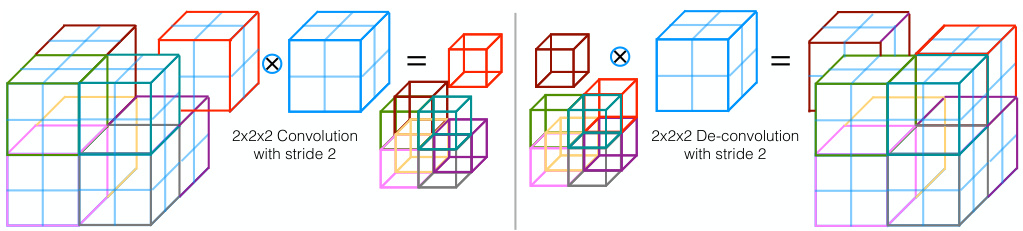
Fig. 3. Convolutions with appropriate stride can be used to reduce the size of the data. Conversely, de-convolutions increase the data size by projecting each input voxel to a bigger region through the kernel.

图 3: 采用适当步长的卷积(convolution)可用于缩减数据尺寸。反卷积(de-convolution)则通过卷积核将每个输入体素(voxel)映射到更大区域，从而增大数据尺寸。

Similarly to [14], we forward the features extracted from early stages of the left part of the CNN to the right part. This is schematically represented in Figure 2 by horizontal connections. In this way we gather fine grained detail that would be otherwise lost in the compression path and we improve the quality of the final contour prediction. We also observed that when these connections improve the convergence time of the model.

与[14]类似，我们将从CNN左侧部分早期阶段提取的特征传递至右侧部分。这一过程在图2中通过水平连接示意呈现。通过这种方式，我们收集了原本会在压缩路径中丢失的细粒度细节，从而提升了最终轮廓预测的质量。我们还观察到，这些连接能缩短模型的收敛时间。

We report in Table 1 the receptive fields of each network layer, showing the fact that the innermost portion of our CNN already captures the content of the whole input volume. We believe that this characteristic is important during segmentation of poorly visible anatomy: the features computed in the deepest layer perceive the whole anatomy of interest at once, since they are computed from data having a spatial support much larger than the typical size of the anatomy we seek to delineate, and therefore impose global constraints.

我们在表1中报告了每个网络层的感受野，表明我们的CNN最内层部分已经捕获了整个输入体积的内容。我们认为这一特性在低可见度解剖结构分割过程中至关重要：最深层计算的特征能一次性感知整个目标解剖结构，因为这些特征是从空间支持远大于我们试图勾勒的典型解剖结构尺寸的数据中计算得出的，因此施加了全局约束。

Table 1. Theoretical receptive field of the $3\times3\times3$ convolutional layers of the network.

表 1: 网络 $3\times3\times3$ 卷积层的理论感受野。

Layer	Input Size	Receptive Field	Layer	Input Size	Receptive Field
L-Stage 1	128	5×5×5	R-Stage 4	16	476 × 476 × 476
L-Stage 2	64	22×22×22	R-Stage 3	32	528×528×528
L-Stage 3	32	72 × 72 × 72	R-Stage 2	64	546×546 × 546
L-Stage 4	16	172 × 172 × 172	R-Stage 1	128	551×551×551
L-Stage 5	8	372×372×372	Output	128	551×551×551

3 Dice loss layer

3 Dice损失层

The network predictions, which consist of two volumes having the same resolution as the original input data, are processed through a soft-max layer which outputs the probability of each voxel to belong to foreground and to background. In medical volumes such as the ones we are processing in this work, it is not uncommon that the anatomy of interest occupies only a very small region of the scan. This often causes the learning process to get trapped in local minima of the loss function yielding a network whose predictions are strongly biased towards background. As a result the foreground region is often missing or only partially detected. Several previous approaches resorted to loss functions based on sample re-weighting where foreground regions are given more importance than background ones during learning. In this work we propose a novel objective function based on dice coefficient, which is a quantity ranging between 0 and 1 which we aim to maximise. The dice coefficient $D$ between two binary volumes can be written as

网络预测结果由两个与原始输入数据分辨率相同的体数据组成，通过soft-max层处理后输出每个体素属于前景和背景的概率。在我们处理的医学体数据中，目标解剖结构往往只占据扫描区域的极小部分。这常导致学习过程陷入损失函数的局部最小值，使网络预测结果严重偏向背景。其结果是前景区域经常缺失或仅被部分检测到。先前多种解决方案采用基于样本加权的损失函数，在学习过程中赋予前景区域更高权重。本文提出一种基于dice系数的新型目标函数，该系数取值范围为0到1，我们的目标是使其最大化。两个二值体数据间的dice系数$D$可表示为

$$
D=\frac{2\sum_{i}^{N}p_{i}g_{i}}{\sum_{i}^{N}p_{i}^{2}+\sum_{i}^{N}g_{i}^{2}}
$$

$$
D=\frac{2\sum_{i}^{N}p_{i}g_{i}}{\sum_{i}^{N}p_{i}^{2}+\sum_{i}^{N}g_{i}^{2}}
$$

where the sums run over the $N$ voxels, of the predicted binary segmentation volume $p_{i}\in P$ and the ground truth binary volume $g_{i}\in G$ . This formulation of Dice can be differentiated yielding the gradient

其中求和运算遍历 $N$ 个体素，分别对应预测的二值分割体积 $p_{i}\in P$ 和真实二值体积 $g_{i}\in G$。这种 Dice 公式可微分从而得到梯度

$$
\frac{\partial D}{\partial p_{j}}=2\left[\frac{g_{j}\left(\sum_{i}^{N}p_{i}^{2}+\sum_{i}^{N}g_{i}^{2}\right)-2p_{j}\left(\sum_{i}^{N}p_{i}g_{i}\right)}{\left(\sum_{i}^{N}p_{i}^{2}+\sum_{i}^{N}g_{i}^{2}\right)^{2}}\right]
$$

$$
\frac{\partial D}{\partial p_{j}}=2\left[\frac{g_{j}\left(\sum_{i}^{N}p_{i}^{2}+\sum_{i}^{N}g_{i}^{2}\right)-2p_{j}\left(\sum_{i}^{N}p_{i}g_{i}\right)}{\left(\sum_{i}^{N}p_{i}^{2}+\sum_{i}^{N}g_{i}^{2}\right)^{2}}\right]
$$

computed with respect to the $j$ -th voxel of the prediction. Using this formulation we do not need to assign weights to samples of different classes to establish the right balance between foreground and background voxels, and we obtain results that we experimentally observed are much better than the ones computed through the same network trained optimising a multi no mi al logistic loss with sample re-weighting (Fig. 6).

相对于预测的第$j$个体素计算。采用这种公式时，我们无需为不同类别的样本分配权重来建立前景与背景体素间的平衡，且通过实验观察到，其结果明显优于通过相同网络优化多名义逻辑损失（带样本重加权）得到的结果（图 6）。

3.1 Training

3.1 训练

Our CNN is trained end-to-end on a dataset of prostate scans in MRI. An example of the typical content of such volumes is shown in Figure 1. All the volumes processed by the network have fixed size of $128\times128\times64$ voxels and a spatial resolution of $1\times1\times1.5$ millimeters.

我们的CNN在MRI前列腺扫描数据集上进行了端到端训练。图1展示了此类体积数据的典型内容示例。网络处理的所有体积数据都具有固定的$128\times128\times64$体素尺寸和$1\times1\times1.5$毫米的空间分辨率。

Annotated medical volumes are not easy to obtain due to the fact that one or more experts are required to manually trace a reliable ground truth annotation and that there is a cost associated with their acquisition. In this work we found necessary to augment the original training dataset in order to obtain robustness and increased precision on the test dataset.

由于获取标注医学影像需要一名或多名专家手动绘制可靠的基准标注，且存在采集成本，这类数据并不易得。在本研究中，我们发现有必要对原始训练数据集进行增强，以提高测试数据集上的鲁棒性和精度。

During every training iteration, we fed as input to the network randomly deformed versions of the training images by using a dense deformation field obtained through a $2\times2\times2$ grid of control-points and B-spline interpolation. This augmentation has been performed ”on-the-fly”, prior to each optimisation iteration, in order to alleviate the otherwise excessive storage requirements. Additionally we vary the intensity distribution of the data by adapting, using histogram matching, the intensity distributions of the training volumes used in each iteration, to the ones of other randomly chosen scans belonging to the dataset.

在每次训练迭代中，我们通过使用从$2\times2\times2$控制点网格和B样条插值获得的密集形变场，向网络输入随机形变后的训练图像版本。这种数据增强在每次优化迭代前"实时"执行，以缓解原本过高的存储需求。此外，我们通过直方图匹配调整每次迭代所用训练数据的强度分布，使其与数据集中随机选取的其他扫描图像的强度分布一致。

3.2 Testing

3.2 测试

A Previously unseen MRI volume can be segmented by processing it in a feedforward manner through the network. The output of the last convolutional layer, after soft-max, consists of a probability map for background and foreground. The voxels having higher probability $\mathrm{\mathit{\Omega}}^{\prime}>0.5\mathrm{\mathit{\Omega}}$ to belong to the foreground than to the background are considered part of the anatomy.

通过前馈方式将先前未见过的MRI体积输入网络进行处理，即可实现分割。最后一个卷积层经过soft-max运算后输出的结果包含背景与前景的概率图。若体素属于前景的概率高于背景(即满足$\mathrm{\mathit{\Omega}}^{\prime}>0.5\mathrm{\mathit{\Omega}}$)，则判定为解剖结构组成部分。

4 Results

4 结果

Fig. 4. Qualitative results on the PROMISE 2012 dataset [7].

图 4: PROMISE 2012数据集[7]上的定性结果。

We trained our method on 50 MRI volumes, and the relative manual ground truth annotation, obtained from the ”PROMISE 2012” challenge dataset [7]. This dataset contains medical data acquired in different hospitals, using different equipment and different acquisition protocols. The data in this dataset is representative of the clinical variability and challenges encountered in clinical settings. As previously stated we massively augmented this dataset through random transformation performed in each training iteration, for each mini-batch fed to the network. The mini-batches used in our implementation contained two volumes each, mainly due to the high memory requirement of the model during training. We used a momentum of 0.99 and a initial learning rate of 0.0001 which decreases by one order of magnitude every 25K iterations.

我们在50个MRI(磁共振成像)体积数据上训练了我们的方法，这些数据及其相对的手动标注真值来自"PROMISE 2012"挑战数据集[7]。该数据集包含从不同医院、使用不同设备和不同采集协议获取的医学数据，能够很好地代表临床实践中遇到的变异性和挑战。如前所述，我们通过在每次训练迭代中对输入网络的每个小批量数据执行随机变换，对该数据集进行了大规模增强。由于模型训练时内存需求较高，我们实现中使用的小批量每个包含两个体积数据。我们采用了0.99的动量和0.0001的初始学习率，该学习率每25K次迭代会降低一个数量级。

Fig. 5. Distribution of volumes with respect to the Dice coefficient achieved during segmentation.

图 5: 基于分割过程中 Dice 系数 (Dice coefficient) 的体积分布。

We tested V-Net on 30 MRI volumes depicting prostate whose ground truth annotation was secret. All the results reported in this section of the paper were obtained directly from the organisers of the challenge after submitting the segmentation obtained through our approach. The test set was representative of the clinical variability encountered in prostate scans in real clinical settings [7].

我们在30个标注真实值保密的前列腺MRI体积数据上测试了V-Net。本文这部分报告的所有结果都是在提交通过我们方法获得的分割结果后，直接从挑战赛组织方获得的。该测试集代表了真实临床环境中前列腺扫描遇到的临床变异性 [7]。

We evaluated the approach performance in terms of Dice coefficient, Hausdorff distance of the predicted delineation to the ground truth annotation and in terms of score obtained on the challenge data as computed by the organisers of ”PROMISE 2012” [7]. The results are shown in Table 2 and Fig. 5.

我们在 Dice 系数、预测轮廓与真实标注的豪斯多夫距离 (Hausdorff distance) 以及 "PROMISE 2012" [7] 主办方计算的挑战数据得分方面评估了该方法性能。结果如表 2 和图 5 所示。

Table 2. Quantitative comparison between the proposed approach and the current best results on the PROMISE 2012 challenge dataset.

Algorithm	Avg.Dice	Avg.Hausdorff distance	Score on challenge task
V-Net+Dice-basedIoss	0.869±0.033	5.71 ± 1.20 mm	82.39
V-Net+mult.logisticloss0.739 ± 0.088		10.55±5.38mm	63.30
Imorphics [18]	0.879 ± 0.044	5.935± 2.14 mm	84.36
ScrAutoProstate	0.874± 0.036	5.58± 1.49 mm	83.49
SBIA	0.835± 0.055	7.73±2.68mm	78.33
Grislies	0.834±0.082	7.90±3.82mm	77.55

表 2. 所提方法与PROMISE 2012挑战数据集当前最佳结果的定量对比

算法	平均Dice系数	平均豪斯多夫距离	挑战任务得分
V-Net+Dice-basedIoss	0.869±0.033	5.71 ± 1.20 mm	82.39
V-Net+mult.logisticloss0.739 ± 0.088		10.55±5.38mm	63.30
Imorphics [18]	0.879 ± 0.044	5.935± 2.14 mm	84.36
ScrAutoProstate	0.874± 0.036	5.58± 1.49 mm	83.49
SBIA	0.835± 0.055	7.73±2.68mm	78.33
Grislies	0.834±0.082	7.90±3.82mm	77.55

Fig. 6. Qualitative comparison between the results obtained using the Dice coefficient based loss (green) and re-weighted soft-max with loss (yellow).

图 6: 基于 Dice 系数损失 (绿色) 和重加权 soft-max 损失 (黄色) 所得结果的定性对比。

Our implementation $^5$ was realised in python, using a custom version of the Caffe $^6$ [5] framework which was enabled to perform volumetric convolutions via CuDNN v3. All the trainings and experiments were ran on a standard workstation equipped with 64 GB of memory, an Intel(R) Core(TM) i7-5820K CPU working at 3.30GHz, and a NVidia GTX 1080 with 8 GB of video memory. We let our model train for 48 hours, or 30K iterations circa, and we were able to segment a previously unseen volume in circa 1 second. The datasets were first normalised using the N4 bias filed correction function of the ANTs framework [17] and then resampled to a common resolution of $1\times1\times1.5$ mm. We applied random deformations to the scans used for training by varying the position of the control points with random quantities obtained from gaussian distribution with zero mean and 15 voxels standard deviation. Qualitative results can be seen in Fig. 4.

我们的实现$^5$采用Python语言完成，基于定制版Caffe$^6$[5]框架，通过CuDNN v3实现体积卷积运算。所有训练和实验均在标准工作站进行，配置包括64GB内存、主频3.30GHz的Intel(R) Core(TM) i7-5820K CPU，以及8GB显存的NVidia GTX 1080显卡。模型训练持续48小时（约3万次迭代），对新体积数据的推理耗时约1秒。数据集首先通过ANTs框架[17]的N4偏置场校正功能进行标准化，随后重采样至$1\times1\times1.5$ mm的统一分辨率。训练过程中对扫描数据施加随机形变，控制点位移量采样自零均值、15体素标准差的高斯分布。定性结果见图4。

5 Conclusion

5 结论

We presented and approach based on a volumetric convolutional neural network that performs segmentation of MRI prostate volumes in a fast and accurate manner. We introduced a novel objective function that we optimise during training based on the Dice overlap coefficient between the predicted segmentation and the ground truth annotation. Our Dice loss layer does not need sample re-weighting when the amount of background and foreground pixels is strongly unbalanced and is indicated for binary segmentation tasks. Although we inspired our architecture to the one proposed in [14], we divided it into stages that learn residuals and, as empirically observed, improve both results and convergence time. Future works will aim at segmenting volumes containing multiple regions in other modalities such as ultrasound and at higher resolutions by splitting the network over multiple GPUs.

我们提出了一种基于体积卷积神经网络的方法，能够快速准确地完成MRI前列腺体积分割。我们引入了一种新颖的目标函数，在训练过程中基于预测分割与真实标注之间的Dice重叠系数进行优化。当背景与前景像素数量严重不平衡时，我们的Dice损失层无需样本重新加权，适用于二值分割任务。虽然我们的架构灵感来源于[14]提出的方案，但将其划分为学习残差的阶段，实证表明这能同时提升结果质量和收敛速度。未来工作将致力于分割超声等其他模态下包含多区域的体积数据，并通过多GPU并行实现更高分辨率的分割。