Enhancing Temporal Action Localization: Advanced S6 Modeling with Recurrent Mechanism
提升时序动作定位:采用循环机制的高级S6建模
Abstract
摘要
Temporal Action Localization(TAL)is a critical task in video analysis,identifying precise start and end times of actions.Existing methods like CNNs,RNNs,GCNs,and Transformers have limitations in capturing long-range depen den cie s and temporal causality.To address these challenges, we propose a novel TAL architecture leveraging the Selective State Space Model (S6). Our approach integrates the Feature Aggregated Bi-S6 block, Dual Bi-S6 structure,and a recurrent mechanism to enhance temporal and channel-wise dependency modeling without increasing parameter complexity.Extensive experiments on bench- mark datasets demonstrate state-of-the-art results with mAP scoresof $74.2%$ onTHUMOS-14, $42.9%$ on Activity Net, $29.6%$ on Fine Action,and $45.8%$ onHACS.Abl ation studies validate our method's effectiveness, showing that the Dual structure in the Stem module and there current me chanism outperform traditional approaches. Our findings demonstrate the potential of S 6-based models in TAL tasks, paving the way for future research.Our code is available at https://github.Com/1sy0882/RDFA-S6.
时序动作定位 (Temporal Action Localization, TAL) 是视频分析中的关键任务,旨在精准识别动作的起止时间。现有方法如 CNN、RNN、GCN 和 Transformer 在捕捉长程依赖与时序因果关系方面存在局限。为解决这些问题,我们提出了一种基于选择性状态空间模型 (Selective State Space Model, S6) 的新型 TAL 架构。该方案通过特征聚合双 S6 模块 (Feature Aggregated Bi-S6)、双路 S6 结构 (Dual Bi-S6) 和循环机制增强时序与通道依赖建模,同时保持参数复杂度不变。在基准数据集上的大量实验取得了领先成果:THUMOS-14 上 mAP 达 $74.2%$,Activity Net 达 $42.9%$,Fine Action 达 $29.6%$,HACS 达 $45.8%$。消融实验验证了方法的有效性,表明主干模块中的双路结构和循环机制优于传统方案。我们的研究证明了基于 S6 的模型在 TAL 任务中的潜力,为未来研究开辟了新方向。代码已开源:https://github.com/1sy0882/RDFA-S6。
1. Introduction
1. 引言
Temporal Action Localization (TAL) is a crucial video analysis task that identifies the precise start and end times of actions in videos. As video content becomes increasingly complex and abundant, accurate TAL methods are essential for effectively capturing and analyzing meaningful actions in applications like sports analytics, surveillance, and interactive media [4, 15, 23,43]. However, significant challenges remain in TAL, particularly in effectively capturing longrange dependencies and temporal causality in video data.
时序动作定位 (Temporal Action Localization, TAL) 是视频分析中的关键任务,旨在识别视频中动作的精确开始和结束时间。随着视频内容日益复杂且海量增长,精准的TAL方法对于体育分析、安防监控和互动媒体等应用场景中有效捕捉与分析有意义动作至关重要 [4, 15, 23,43]。然而TAL仍面临重大挑战,尤其是在有效捕捉视频数据中的长程依赖关系与时序因果关系方面。
Traditional approaches to TAL, including CNNs, RNNs, GCNs, and Transformers, each bring unique strengths but also have inherent limitations. CNNs are effective at capturing spatial features but struggle with long-range dependencies due to limited receptive fields [31]. RNNs can model temporal sequences but face challenges such as vanishing gradients, which hinder their ability to capture long-term dependencies [10, 26]. GCNs are powerful for relational data but are not inherently designed for sequential temporal data [17]. Transformers have revolutionized TAL with their ability to model global context using self-attention mechanisms [2, 32]. However, their reliance on attention scores to capture relationships within a sequence does not inherently account for the temporal causality and history of visual elements over time. This limitation makes Transformers less optimal for tasks requiring precise temporal causality, such as TAL, where understanding the sequential nature and dependencies of actions is crucial [11, 13].
传统时序动作定位(TAL)方法包括CNN、RNN、GCN和Transformer,各具优势但存在固有局限。CNN擅长捕捉空间特征,却因感受野有限而难以建模长程依赖[31]。RNN可建模时序关系,但存在梯度消失等问题,影响长时依赖捕捉[10,26]。GCN虽擅长处理关系数据,却非为时序数据设计[17]。Transformer通过自注意力机制建模全局上下文,革新了该领域[2,32],但其依赖注意力分数建模序列关系时,未显式考虑视觉元素随时间变化的时序因果性,因此在需要精确时序因果关系的任务(如时序动作定位)中表现欠佳[11,13]——这类任务中理解动作序列性质与依赖关系至关重要。
The State Space Model (SSM) [11, 13] has emerged as a promising alternative for sequence modeling by addressing the limitations of traditional methods, especially in capturing temporal causality. Within the SSM framework, the Selective State Space Model (S6) [11] stands out for TAL tasks due to its ability to maintain and leverage historical context through its selection mechanism and gating operation. These properties enable S6 to dynamically adjust the influence of new inputs—specifically, the s patio temporal feature vectors extracted from the current video clip——ensuring that the model retains and utilizes critical temporal information while integrating new data. This dynamic adjustment and selective retention enable S6 to capture long-range dependencies and temporal causality effectively, providing understanding of action sequences essential for accurately pinpointing the start and end times of actions in TAL.
状态空间模型 (State Space Model, SSM) [11, 13] 通过解决传统方法的局限性(尤其是在捕捉时序因果关系方面),已成为序列建模的一种有前景的替代方案。在 SSM 框架中,选择性状态空间模型 (Selective State Space Model, S6) [11] 因其通过选择机制和门控操作保持并利用历史上下文的能力,在时序动作定位 (TAL) 任务中表现突出。这些特性使 S6 能够动态调整新输入(即从当前视频片段提取的时空特征向量)的影响,确保模型在整合新数据的同时保留并利用关键的时序信息。这种动态调整和选择性保留使 S6 能有效捕捉长程依赖和时序因果关系,从而为准确判定 TAL 任务中动作的起止时间提供对动作序列的深刻理解。
Action Mamba [7], an S6-based TAL method, has demonstrated that S6-based method can surpass Transformers in sequence modeling by replacing Transformer blocks with S6 blocks. Action Mamba simply substitutes the Transformer-based blocks for sequence modeling in the ActionFormer [42] architecture with S6-based blocks. The S6 blocks use a bi-directional processing approach [45] and incorporate weight sharing between networks operating in each direction. However, this study lacks a thoughtful design focused on effective TAL methods, instead offering a straightforward replacement of Transformer blocks with slightly enhanced S6 ones. While Action Mamba highlights the potential for S6-based sequence modeling to outperform Transformer-based approaches, it falls short of fully exploring this potential or providing clear guidelines for leveraging S6 effectively in TAL tasks.
Action Mamba [7]是一种基于S6的时序动作定位(TAL)方法,其研究表明通过用S6模块替代Transformer模块,基于S6的方法在序列建模上可以超越Transformer。该方法直接将ActionFormer [42]架构中基于Transformer的序列建模模块替换为S6模块。S6模块采用双向处理机制 [45],并在两个方向的网络间实现权重共享。但该研究缺乏针对高效TAL方法的深思熟虑设计,仅提供了对Transformer模块的简单替换方案,且S6模块仅做了轻微改进。虽然Action Mamba证明了基于S6的序列建模具有超越Transformer方法的潜力,但既未充分挖掘这种潜力,也未就如何有效运用S6处理TAL任务给出明确指导。
Our research aims to explore the potential of S6-based TAL methods by building on insights from previous studies on CNNs, RNNs, GCNs, and Transformers [10,17,26,31,32]. We propose a novel architecture that leverages the strengths of these traditional models while capitalizing on the unique capabilities of S6.
我们的研究旨在基于先前对CNN、RNN、GCN和Transformer [10,17,26,31,32] 的研究见解,探索基于S6的TAL方法的潜力。我们提出了一种新颖的架构,既能利用这些传统模型的优势,又能充分发挥S6的独特能力。
This paper makes the following contributions to the field ofTAL:
本文对TAL领域做出以下贡献:
- Advanced Dependency Modeling with S6: We conduct a pioneering exploration of S6's potential in TAL tasks, particularly focusing on its dependency modeling capabilities. By introducing an advanced dependency modeling technique based on the Feature Aggregated Bi-S6 (FA-Bi-S6) block design and the Dual Bi-S6 structure, we enable robust and effective modeling of dependencies within video sequences. The FA-Bi-S6 block employs multiple Conv1D layers with different kernel sizes to capture various granular i ties of temporal and channel-wise features, while the Dual Bi-S6 structure processes features along both the temporal and channel dimensions to enhance the integration of s patio temporal dependencies. This approach provides direction for TAL modeling, enabling more effective utilization of S6 in this domain.
- 基于S6的高级依赖建模:我们开创性地探索了S6在时序动作定位(TAL)任务中的潜力,重点研究其依赖建模能力。通过引入基于特征聚合双向S6(FA-Bi-S6)块设计和双重双向S6结构的先进依赖建模技术,我们实现了对视频序列内部依赖关系的稳健有效建模。FA-Bi-S6块采用多个不同卷积核尺寸的Conv1D层来捕获时间和通道特征的多粒度信息,而双重双向S6结构则沿时间和通道双维度处理特征,以增强时空依赖的整合。该方法为TAL建模提供了新方向,使S6在该领域得到更有效的应用。
- Efficiency through Recurrent Mechanism: Our study reveals that using a recurrent mechanism to repeatedly apply a single S6-based model outperforms the traditional approach of stacking multiple blocks. This recurrent application enhances the model's performance without increasing the number of parameters, providing an effective solution for improving TAL models.
- 通过循环机制提升效率:我们的研究表明,采用循环机制重复应用单一基于S6的模型,其效果优于传统的堆叠多个模块的方法。这种循环应用在不增加参数量的情况下提升了模型性能,为改进TAL (Temporal Action Localization) 模型提供了有效解决方案。
- State-of-the-Art Performance: We achieve stateof-the-art (SOTA) results across multiple benchmark datasets, including THUMOS-14 [15], Activity Net [4], FineAction [23], and HACS [43]. Our ablation studies analyze the effectiveness of each component of our proposed architecture, confirming the performance improvements brought by our method.
- 领先性能表现:我们在多个基准数据集上实现了最先进 (state-of-the-art, SOTA) 的结果,包括 THUMOS-14 [15]、Activity Net [4]、FineAction [23] 和 HACS [43]。通过消融实验分析了所提架构各模块的有效性,验证了本方法带来的性能提升。
2. Related works
2. 相关工作
Convolutional Neural Networks (CNNs) Early TAL research used 2D CNNs to process spatial information, with initial attempts like FV-DTF [25] combining spatial and temporal data but handling them separately. The introduction of 3D CNNs, as seen in CDC [29], marked a significant advancement by capturing s patio temporal features with three-dimensional convolution kernels. However, temporal resolution loss inherent in traditional 3D CNNs was still a challenge to conquer. To cope with this, methods such as TPC [37] and FSN [38] aimed to balance spatial and temporal feature processing. GTAN [24] and PBRNet [20] further optimized temporal intervals and hierarchical feature extraction. TPC maintained temporal receptive fields while down sampling spatial fields, and FSN captured finergrained dependencies by sequentially processing spatial and temporal features.
卷积神经网络 (CNN)
早期TAL研究使用2D CNN处理空间信息,如FV-DTF [25]等初期尝试将时空数据结合但仍分开处理。3D CNN的出现标志着重大进步,如CDC [29]通过三维卷积核捕获时空特征。然而传统3D CNN固有的时间分辨率损失仍是待解难题。为此,TPC [37]和FSN [38]等方法致力于平衡时空特征处理。GTAN [24]与PBRNet [20]进一步优化了时间间隔和分层特征提取:TPC在空间下采样时保持时间感受野,FSN则通过顺序处理时空特征捕获细粒度依赖关系。
Our FA-Bi-S6 block builds on these advances by incorporating multiple Conv1D layers with varying kernel sizes in parallel to capture a wide range of local contexts. The resulting feature map is processed bi-direction ally by the Bi-S6 network, enhancing the model's ability to capture complex dynamics effectively.
我们的FA-Bi-S6模块通过并行整合多个不同卷积核大小的Conv1D层来捕捉广泛的局部上下文,以此为基础实现了性能提升。生成的特征图由Bi-S6网络进行双向处理,有效增强了模型捕捉复杂动态特征的能力。
Recurrent Neural Networks (RNNs)To address the temporal challenges that CNNs alone couldn't solve, RNNs were integrated into TAL frameworks. Early efforts like PSDF [4O] and advancements such as AS [1] used RNNs to enhance temporal context modeling from dense trajectories and refine spatial features for detailed analysis. More sophisticated integration s followed, such as GRU-Split [16], which employed GRUs to refine action boundaries and probabilities. However, RNNs introduced challenges like managing long sequences and vanishing gradients. RCL [34] addressed these issues by using a recurrent module to dynamically adjust action segment predictions.
循环神经网络 (RNNs)
为解决仅靠卷积神经网络 (CNNs) 无法处理的时序问题,RNNs 被引入时序动作定位 (TAL) 框架。早期研究如 PSDF [4O] 和 AS [1] 等改进方案利用 RNNs 增强密集轨迹的时序上下文建模,并优化空间特征以实现精细分析。后续更复杂的集成方案如 GRU-Split [16] 采用门控循环单元 (GRUs) 来优化动作边界和概率预测。但 RNNs 也带来了长序列处理和梯度消失等挑战。RCL [34] 通过循环模块动态调整动作片段预测,有效缓解了这些问题。
Our research transcends the limitations of CNNs and RNNs by incorporating a recurrent mechanism within our S6-based architecture. This mechanism, integrated with our Backbone's Stem module, enhances temporal context modeling using the efficiency and precision of state space models.
我们的研究通过在基于S6的架构中融入循环机制,超越了CNN和RNN的局限性。该机制与主干网络(Backbone)的Stem模块相结合,利用状态空间模型(state space model)的高效性和精确性,增强了时序上下文建模能力。
Graph Convolutional Networks (GCNs)The limitations of RNNs led to the exploration of GCNs in the TAL domain. GCNs structure video data as graphs, with nodes representing s patio temporal features and edges defining their relationships, allowing for more comprehensive modeling of temporal dependencies. A notable advancement, P-GCN [41], expanded the range of dependencies that could be modeled but faced challenges in s cal ability and efficiency due to computational overhead. G-TAD [36] addressed these issues with a dual-stream graph convolution framework, effciently capturing both fixed and adaptive temporal dependencies.
图卷积网络 (GCNs)
RNN的局限性促使人们在TAL领域探索GCN的应用。GCN将视频数据构建为图结构,其中节点表示时空特征,边定义特征间的关系,从而实现对时间依赖关系更全面的建模。P-GCN [41] 作为重要进展扩展了可建模的依赖范围,但因计算开销面临可扩展性和效率方面的挑战。G-TAD [36] 通过双流图卷积框架解决了这些问题,能高效捕获固定和自适应的时序依赖关系。
Building on GCN insights, we developed the Dual Bi-S6 structure, integrating the TFA-Bi-S6 and CFA-Bi-S6 blocks. TFA-Bi-S6 captures temporal dependencies, while CFA-BiS6 handles dependencies between s patio temporal features by focusing on the channel dimension. This combined approach enhances the robustness and accuracy of TAL by effectively modeling both temporal and channel-wise contexts.
基于GCN的洞见,我们开发了Dual Bi-S6结构,整合了TFA-Bi-S6和CFA-Bi-S6模块。TFA-Bi-S6负责捕捉时序依赖关系,而CFA-BiS6则通过聚焦通道维度来处理时空特征间的依赖关系。这种组合方法通过有效建模时序和通道上下文,提升了时序动作定位(TAL)的鲁棒性和准确性。
Transformers The limitations of GCNs in handling extensive temporal dependencies led to the adoption of
Transformer 由于图卷积网络(GCN)在处理长程时间依赖性方面的局限性,研究者转而采用
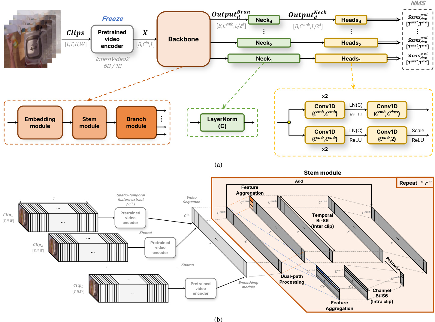
Figure 1. I lust ration of the proposed architecture and its components. (a) The architecture overview, which consists of four main parts: Pretrained video encoder, Backbone, Neck, and Heads (Action classification head and Temporal boundary regression head). (b) The overview of the proposed methods, highlighting the Stem module with an orange shaded area. The Stem module consists of three parts: Dual-path processing (Dual Bi-S6 Structure), Feature Aggregation & Temporal/Channel Bi-S6 (Feature Aggregated Bi-S6 Block Design), and the repeat processing with shared networks (Recurrent Mechanism).
图 1: 提出的架构及其组件示意图。(a) 架构概览,包含四个主要部分:预训练视频编码器 (Pretrained video encoder)、主干网络 (Backbone)、颈部网络 (Neck) 和头部网络 (Heads) (动作分类头 (Action classification head) 和时间边界回归头 (Temporal boundary regression head))。(b) 提出的方法概览,橙色阴影区域突出显示了 Stem 模块。该模块由三部分组成:双路径处理 (Dual-path processing) (双 Bi-S6 结构 (Dual Bi-S6 Structure))、特征聚合与时间/通道 Bi-S6 (Feature Aggregation & Temporal/Channel Bi-S6) (特征聚合 Bi-S6 块设计 (Feature Aggregated Bi-S6 Block Design)) 以及共享网络的重复处理 (Recurrent Mechanism)。
Transformer-based models in TAL. Transformers use selfattention to extend temporal dependencies beyond GCN constraints. TRA [44] used variable temporal boundary pro posals with multi-head self-attention for fexible temporal modeling, though it faced challenges in maintaining temporal causality over long sequences. Action Former [42] improved on this by using local self-attention and a multiscale feature pyramid to capture various temporal resolutions, but it still struggled with capturing long-range dependencies and maintaining precise temporal causality.
TAL中的Transformer模型。Transformer通过自注意力(selfattention)机制将时序依赖关系扩展到超越GCN限制的范围。TRA [44]采用多头自注意力机制的可变时序边界提案实现灵活时序建模,但在维持长序列的时序因果关系方面存在挑战。Action Former [42]通过局部自注意力和多尺度特征金字塔来捕捉不同时间分辨率,对此进行了改进,但在捕获长程依赖关系和保持精确时序因果关系方面仍有不足。
To address these issues, we introduced the S6 network into our TAL system. The S6 network uses selective mechanisms and gating functions to modulate the impact of each time step's s patio temporal features. This approach allows S6 to preserve critical historical information while integrating new s patio temporal features, effectively capturing longrange dependencies and temporal causality. By leveraging these capabilities, S6 enhances the accuracy of feature extraction and action localization, addressing the limitations of Transformer-based models in TAL.
为了解决这些问题,我们在TAL系统中引入了S6网络。S6网络利用选择性机制和门控函数来调节每个时间步的时空特征影响。这种方法使S6能够在整合新时空特征的同时保留关键历史信息,有效捕捉长程依赖关系和时间因果关系。通过利用这些能力,S6提升了特征提取和动作定位的准确性,解决了基于Transformer的模型在TAL中的局限性。
3. Proposed Methods
3. 研究方法
We introduce our approach, emphasizing advanced dependency modeling for TAL by integrating the S6 model to improve long-range dependency handling. Our key components include the Feature Aggregated Bi-S6 Block Design, Dual Bi-S6 Structure, and Recurrent Mechanism.
我们介绍了通过整合S6模型来改进长距离依赖处理的方法,强调TAL(任务自适应学习)中的高级依赖建模。关键组件包括特征聚合双S6模块设计、双S6结构和循环机制。
3.1. Preliminary: Selective Space State Model (S6)
3.1. 预备知识:选择性空间状态模型 (S6)
Our architecture uses theS6 model with selective mechanisms and gating operations to capture complex temporal dynamics and capture long-range dependencies effectively.
我们的架构采用带有选择性机制和门控操作的S6模型,以有效捕捉复杂的时间动态并捕获长程依赖关系。
The S6 model operates with parameters $(\Delta_{t},A,B,C)$
S6模型以参数$(\Delta_{t},A,B,C)$运行
disc ret i zed to manage sequence transformations:
离散化处理以管理序列变换:
$$
h_{t}=A h_{t-1}+B x_{t},\quad y_{t}=C h_{t}
$$
$$
h_{t}=A h_{t-1}+B x_{t},\quad y_{t}=C h_{t}
$$
Here, $x_{t}$ represents the input at time step $t$ , which, in the case of TAL, is the s patio temporal feature vector extracted from single clip. The hidden state at time step $t,h_{t}$ , captures the temporal context of the sequence. The output at time step $t$ $y_{t}$ , represents the processed feature. The state matrix $A$ determines how the previous hidden state $h_{t-1}$ and the historical information from all previous steps influence the current hidden state $h_{t}$ [12], contributing to precise action localization. The input matrix $B$ defines how the input $x_{t}$ affects the hidden state $h_{t}$ ..Finally, the output matrix $C$ translates the hidden state $h_{t}$ into the output $y_{t}$
这里,$x_{t}$ 表示时间步 $t$ 的输入,在 TAL (Temporal Action Localization) 中是从单个片段提取的时空特征向量。时间步 $t$ 的隐藏状态 $h_{t}$ 捕捉了序列的时序上下文。时间步 $t$ 的输出 $y_{t}$ 表示处理后的特征。状态矩阵 $A$ 决定了前一个隐藏状态 $h_{t-1}$ 以及所有先前步骤的历史信息如何影响当前隐藏状态 $h_{t}$ [12],从而有助于精确的动作定位。输入矩阵 $B$ 定义了输入 $x_{t}$ 如何影响隐藏状态 $h_{t}$。最后,输出矩阵 $C$ 将隐藏状态 $h_{t}$ 转换为输出 $y_{t}$。
The process starts with the input $x_{t}$ being projected to derive $B,C$ ,and $\Delta_{t}$ . This step transforms raw input features into suitable representations for state-space modeling. Specifically, the projection functions apply linear transformations to the input $x_{t}$
该过程从输入$x_{t}$开始,通过投影得到$B,C$和$\Delta_{t}$。此步骤将原始输入特征转换为适用于状态空间建模的表示形式。具体而言,投影函数对输入$x_{t}$应用线性变换。
$$
B=\operatorname{Linear}(x_{t}),\quad C=\operatorname{Linear}(x_{t})
$$
$$
B=\operatorname{Linear}(x_{t}),\quad C=\operatorname{Linear}(x_{t})
$$
To dynamically manage information flow, the S6 model employs selection mechanism and gating function. The dynamically adjusted parameter $\Delta_{t}$ controls the disc ret iz ation of the state-space model based on the relevance of the input $x_{t}$ , functioning similarly to a gating mechanism in RNNs. The projection function $s_{\Delta}(x_{t})$ , which includes learnable parameters, projects the input $x_{t}$ to one dimension before broadcasting it across channels:
为动态管理信息流,S6模型采用选择机制和门控函数。动态调整参数$\Delta_{t}$根据输入$x_{t}$的相关性控制状态空间模型的离散化,其功能类似于RNN中的门控机制。包含可学习参数的投影函数$s_{\Delta}(x_{t})$将输入$x_{t}$投影至一维后再进行通道广播:
$$
\Delta_{t}=\mathrm{softplus}(s_{\Delta}(x_{t}))
$$
$$
\Delta_{t}=\mathrm{softplus}(s_{\Delta}(x_{t}))
$$
Next, the disc ret iz ation step adjusts the parameters $A$ and $B$ for the current time step $t$ , ensuring that the parameters are appropriately scaled for discrete-time processing:
接下来,离散化步骤会调整当前时间步长 $t$ 的参数 $A$ 和 $B$,确保这些参数经过适当缩放以适用于离散时间处理:
$$
A_{t}=\exp(\Delta_{t}A)
$$
$$
A_{t}=\exp(\Delta_{t}A)
$$
$$
B_{t}=(\Delta_{t}A)^{-1}(\exp(\Delta_{t}A)-I)\cdot\Delta_{t}B
$$
$$
B_{t}=(\Delta_{t}A)^{-1}(\exp(\Delta_{t}A)-I)\cdot\Delta_{t}B
$$
The hidden state $h_{t}$ is updated using $A_{t}$ and $B_{t}$ , and the output $y_{t}$ is generated using $C_{t}=C$
隐藏状态 $h_{t}$ 通过 $A_{t}$ 和 $B_{t}$ 更新,输出 $y_{t}$ 由 $C_{t}=C$ 生成
$$
h_{t}=A_{t}h_{t-1}+B_{t}x_{t},\quad y_{t}=C_{t}h_{t}
$$
$$
h_{t}=A_{t}h_{t-1}+B_{t}x_{t},\quad y_{t}=C_{t}h_{t}
$$
The selective update of the hidden state can be understood as:
隐藏状态的选择性更新可以理解为:
$$
h_{t}=(1-\Delta_{t})h_{t-1}+\Delta_{t}x_{t}
$$
$$
h_{t}=(1-\Delta_{t})h_{t-1}+\Delta_{t}x_{t}
$$
where $\Delta_{t}$ functions similarly to the gating function $g_{t}$ in RNNs, determining the influence of the input $x_{t}$ on the hidden state $h_{t}$ . This dynamic adjustment helps the model focus on relevant portions of the input, ensuring effective handling of long-range dependencies.
其中 $\Delta_{t}$ 的功能类似于 RNN 中的门控函数 $g_{t}$ ,用于决定输入 $x_{t}$ 对隐藏状态 $h_{t}$ 的影响。这种动态调整机制帮助模型聚焦于输入的相关部分,确保有效处理长距离依赖关系。
S6 is particularly effective in TAL tasks due to its ability to maintain and refine temporal context over extended sequences. By dynamically adjusting $\Delta_{t}$ , the model can selectively retain important temporal features.
S6 在 TAL 任务中特别有效,因为它能够在长序列中保持并优化时间上下文。通过动态调整 $\Delta_{t}$,该模型可以选择性地保留重要的时间特征。
3.2. Overview
3.2. 概述
Our architecture, inspired by Action Former [42] and ActionMamba [7], consists of four primary components: a Pretrained video encoder, a Backbone, a Neck, and Heads. The overview of architecture is depicted in Figure 1a.
我们的架构受 Action Former [42] 和 ActionMamba [7] 启发,包含四个主要组件:预训练视频编码器 (Pretrained video encoder)、主干网络 (Backbone)、颈部网络 (Neck) 和头部网络 (Heads)。架构概览如图 1a 所示。
Pretrained Video EncoderThe Pretrained video encoder extracts s patio temporal attributes from video clips. Trained on diverse datasets such as UCF, Kinetics, SomethingSomething, and vision-language multi-modal datasets like WebVid and InternVid, it leverages the vast training data from Inter Video 2-6B/1B [35]. The pretrained video encoder's example of receiving each clip and extracting spatio temporal features is shown in Appendix A.
预训练视频编码器
预训练视频编码器从视频片段中提取时空特征。该模型在UCF、Kinetics、SomethingSomething等多样化数据集,以及WebVid、InternVid等视觉-语言多模态数据集上进行训练,并利用了Inter Video 2-6B/1B [35]的海量训练数据。预训练视频编码器接收每个片段并提取时空特征的示例如附录A所示。
Backbone The Backbone captures dependencies and extracts features at various temporal resolutions from the sequence data. As illustrated in Figure 1a, it consists of three main modules:
主干网络
主干网络用于捕捉序列数据中的依赖关系,并从不同时间分辨率中提取特征。如图 1a 所示,它由三个主要模块组成:
· Embedding Module: This module captures the coarse local context of s patio temporal features. As shown in Figure 2a, the sequence is first passed through a Conv1D to increase the dimensionality from $C^{i n}$ to $C^{e m b}$ , followed by Layer Normalization (LN) and ReLU activation. This process is followed by $B_{e}$ sequential Conv1D with dimensions $C^{e m b}$ to $C^{e m b}$ , each followed by LN and ReLU activation, resulting in an embedded sequence of shape $[B,C^{e m b},L]$
· 嵌入模块 (Embedding Module):该模块用于捕捉时空特征的粗略局部上下文。如图 2a 所示,序列首先通过 Conv1D 将维度从 $C^{i n}$ 提升至 $C^{e m b}$,随后进行层归一化 (LN) 和 ReLU 激活。接着经过 $B_{e}$ 个连续的 Conv1D 层(维度保持 $C^{e m b}$ 到 $C^{e m b}$),每层后接 LN 和 ReLU 激活,最终生成形状为 $[B,C^{e m b},L]$ 的嵌入序列。
· Stem Module: This core component processes the embedded sequences to capture long-range dependency using the Dual Bi-S6 Structure. As shown in Figure 2b, it applies two main blocks in parallel: the Temporal Feature Aggregated Bi-S6 (TFA-Bi-S6) block and the Channel Feature Aggregated Bi-S6 (CFA-Bi-S6) block, which focus on capturing temporal and channel-wise dependencies, respectively. Each of these blocks is stacked $B_{s}$ times. The TFA-Bi-S6 block handles input sequences reshaped from $[B,C^{e m b},L]$ to $[B,L,C^{e m b}]$ and outputs back to $[B,C^{e m b},L]$ . The CFA-Bi-S6 block processes the temporal-pooled output of TFABi-S6 with shape $[B,C^{e m b},1]$ and scales it using a sigmoid activation. The outputs from these blocks are combined through point-wise multiplication with the TFA-Bi-S6 output. This combined output then goes through an affine transformation with a drop path and skip connection, followed by LN to enhance capacity. This process uses a Recurrent Mechanism, repeating $r$ times, with a weight-shared network applied at each repetition to refine temporal dependency modeling.
· Stem模块:该核心组件通过Dual Bi-S6结构处理嵌入序列以捕获长程依赖。如图2b所示,它并行应用两个主要模块:专注于时间依赖的时序特征聚合Bi-S6 (TFA-Bi-S6) 模块和专注于通道依赖的通道特征聚合Bi-S6 (CFA-Bi-S6) 模块,每个模块均堆叠 $B_{s}$ 次。TFA-Bi-S6模块将输入序列从 $[B,C^{e m b},L]$ 重塑为 $[B,L,C^{e m b}]$ 并输出回 $[B,C^{e m b},L]$ 。CFA-Bi-S6模块处理TFA-Bi-S6输出的时序池化结果(形状 $[B,C^{e m b},1]$ ),并使用sigmoid激活函数进行缩放。这些模块的输出通过逐点乘法与TFA-Bi-S6输出结合,随后经过带drop path和跳跃连接的仿射变换,再通过LN层增强容量。该过程采用循环机制重复 $r$ 次,每次迭代应用权重共享网络以优化时序依赖建模。
· Branch Module: This module handles temporal multi- scale dependencies. As shown in Figure 2c, each branch applies the Temporal Bi-S6 (T-Bi-S6) block, which is a modified version of the Bi-S6 block used in ActionMamba [7], followed by an affine drop path and residual connection. After this, the output undergoes LN and max pooling along the temporal dimension, effectively obtaining various temporal resolutions. The T-BiS6 block processes the input sequence reshaped from $[B,C^{e m b},L/2^{d-1}]$ to $[B,L/2^{d-1},C^{e m b}]$ and outputs back to $[B,C^{e m b},L/2^{d-1}]$ . This process is repeated for each down sampling index $(d=1,2,...,5)$ , where the output shape becomes $[B,C^{e m b},L/2^{d}]$
· 分支模块:该模块处理时间多尺度依赖关系。如图 2c 所示,每个分支应用 Temporal Bi-S6 (T-Bi-S6) 块(这是对 ActionMamba [7] 中使用的 Bi-S6 块的改进版本),后接仿射丢弃路径和残差连接。之后,输出沿时间维度进行层归一化 (LN) 和最大池化,从而有效获取不同时间分辨率。T-BiS6 块将输入序列从 $[B,C^{e m b},L/2^{d-1}]$ 重塑为 $[B,L/2^{d-1},C^{e m b}]$ 并输出回 $[B,C^{e m b},L/2^{d-1}]$。该过程对每个下采样索引 $(d=1,2,...,5)$ 重复执行,最终输出形状变为 $[B,C^{e m b},L/2^{d}]$。
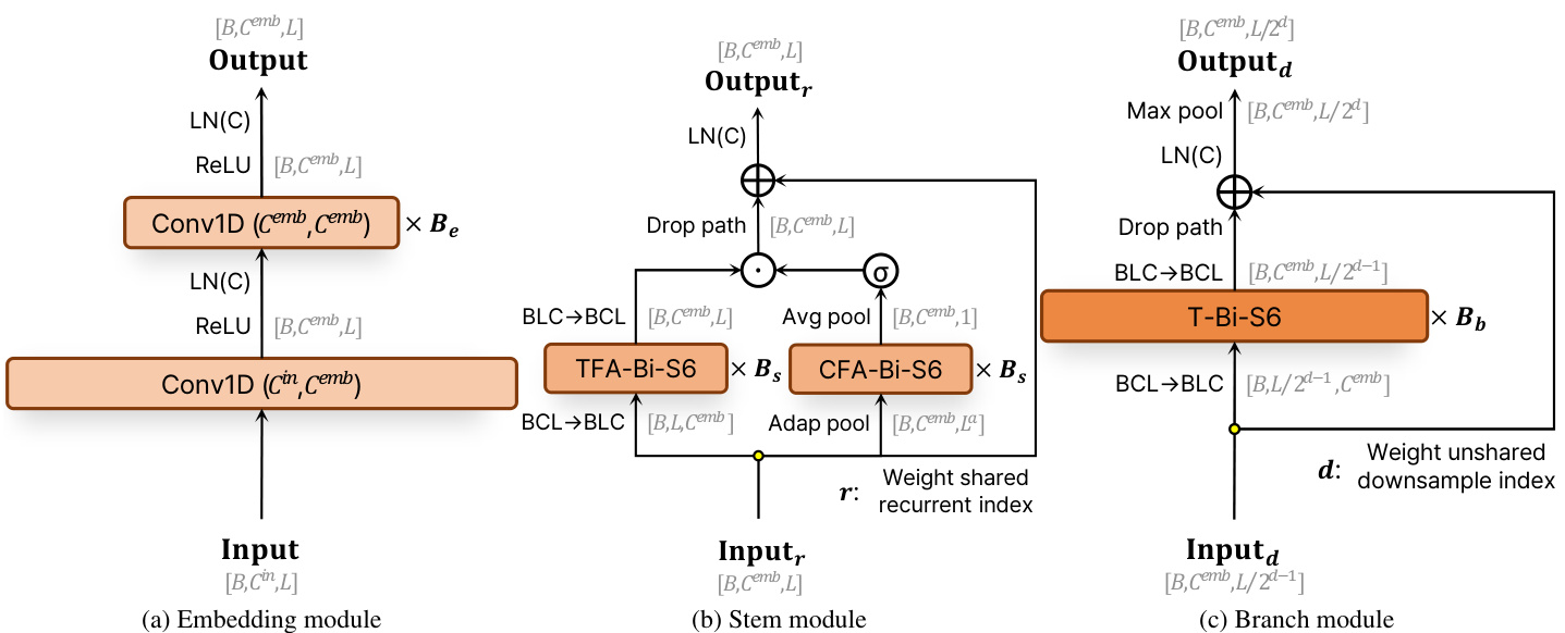
Figure 2. Diagrams of the Embedding, Stem, and Branch modules. (a) Embedding module. (b) Stem module. (c) Branch module.
图 2: 嵌入模块、主干模块和分支模块的示意图。(a) 嵌入模块。(b) 主干模块。(c) 分支模块。
Neck and Heads The Neck is designed with simplicity and efficiency in mind, utilizing layer normalization for channelwise normalization, which is the same as the LN used in the Branch module. This step ensures that the temporal multiscale sequences reflecting precise temporal dependencies processed by the Backbone are normalized and ready for subsequent processing.
颈部和头部
颈部的设计注重简洁高效,采用层归一化(layer normalization)进行通道归一化,与分支模块中使用的LN相同。这一步骤确保由主干网络处理的反映精确时间依赖性的时序多尺度序列经过归一化,为后续处理做好准备。
The Heads leverage the normalized features from the Neck to carry out two primary tasks: action classification and temporal boundary regression. The action classification head generates channels equal to the number of action categories, predicting class scores for each category. Simultaneously, the temporal boundary regression head outputs two channels to predict the frame indices marking the start and end of an action. This dual-head design ensures that the model can accurately classify actions and determine their temporal boundaries within the video segments.
头部利用来自颈部的归一化特征执行两项主要任务:动作分类和时间边界回归。动作分类头生成与动作类别数量相等的通道,预测每个类别的得分。同时,时间边界回归头输出两个通道,用于预测标记动作开始和结束的帧索引。这种双头设计确保模型能够准确分类动作并确定其在视频片段中的时间边界。
3.3. Advanced Dependency Modeling for TAL
3.3. TAL 高级依赖建模
Feature Aggregated Bi-S6 (FA-Bi-S6) Block Design The FA-Bi-S6 block design is one of our contributions, enabling robust and effective modeling of dependencies within video sequences. This block design incorporates multiple Conv1D layers, each with different kernel sizes, operating sequentially within two main blocks: the TFA-Bi-S6 block and the CFA-Bi-S6 block, as shown in Figure 3a and 3b.
特征聚合双向S6 (FA-Bi-S6) 模块设计
FA-Bi-S6模块设计是我们的贡献之一,能够对视频序列中的依赖关系进行鲁棒且有效的建模。该模块设计包含多个具有不同卷积核尺寸的Conv1D层,这些层在两个主要模块中依次运行:TFA-Bi-S6模块和CFA-Bi-S6模块,如图3a和3b所示。
In the TFA-Bi-S6 block, the input sequence of shape $[B,C^{e m b},L]$ is first passed through a linear layer that ad justs the dimensions from $[B,C^{e m b},L]$ to $[B,L,2C^{e m b}]$ The sequence is then divided into two chunks, and one of these chunks is fipped. These chunks are processed through multiple Conv1D layers with varying kernel sizes (2, 3, 4), each capturing different granular i ties of temporal features. The outputs from these Conv1D layers are summed to create an aggregated feature map, which is then processed through a S6 network focusing on temporal dependencies. The output of the S6 blocks is then multiplied pointwise with the original chunked input processed through the SiLU activation. The results from each chunk are concatenated, which handle bi-directional temporal dependencies. The final output is obtained by combining the results, which are then processed through a linear layer and reshaped back to $[B,C^{e m b},L]$
在 TFA-Bi-S6 模块中,形状为 $[B,C^{e m b},L]$ 的输入序列首先通过一个线性层,将维度从 $[B,C^{e m b},L]$ 调整为 $[B,L,2C^{e m b}]$。随后,该序列被分成两部分,其中一部分进行翻转。这些分块通过多个具有不同核大小 (2, 3, 4) 的 Conv1D 层处理,每个层捕获不同粒度的时间特征。这些 Conv1D 层的输出被求和以创建聚合特征图,然后通过专注于时间依赖性的 S6 网络进行处理。S6 块的输出随后与通过 SiLU 激活处理的原始分块输入进行逐点相乘。每个分块的结果被拼接起来,以处理双向时间依赖性。最终输出通过将结果组合后,再经过线性层处理并重塑回 $[B,C^{e m b},L]$ 的形状得到。
In the CFA-Bi-S6 block, the process is similar to the TFABi-S6 block with adaptations for channel-wise dependency modeling. The input sequence is first adaptively pooled to $[B,C^{e m b},L^{a}]$ before the linear layer processing. The Conv1D layers in this block have varying kernel sizes (2, 4, 8) to capture different scales of channel-wise dependencies. After processing through the S6 blocks and linear layer, the final output is average pooled to $[B,C^{e m b},1]$ .These adjustments enable the CFA-Bi-S6 block to focus on capturing diverse channel-wise dependencies and enhance the overall capacity to model complex s patio temporal interactions within video sequences.
在CFA-Bi-S6模块中,其流程与TFABi-S6模块类似,但针对通道级依赖建模进行了调整。输入序列首先通过自适应池化处理为$[B,C^{e m b},L^{a}]$,随后进入线性层。该模块中的Conv1D层采用不同卷积核尺寸(2, 4, 8)以捕获多尺度通道级依赖关系。经过S6模块和线性层处理后,最终输出通过平均池化降维至$[B,C^{e m b},1]$。这些调整使CFA-Bi-S6模块能够专注于捕捉多样化的通道级依赖关系,并增强对视频序列中复杂时空交互的建模能力。
By integrating the Bi-S6 block with the aggregated feature map, our design leverages the strengths of both multiscale feature extraction and bi-directional processing. The combined architecture allows the model to effectively capture and utilize s patio temporal features across a wide range of context, addressing the limitations of traditional single convolutional approaches. This design is particularly advantageous for TAL tasks, where actions may occur over varying temporal spans, and the local context provided by surrounding frames is crucial for accurate localization.
通过将Bi-S6模块与聚合特征图相结合,我们的设计充分利用了多尺度特征提取和双向处理的优势。这种组合架构使模型能够有效捕获并利用跨广泛上下文的时空特征,解决了传统单一卷积方法的局限性。该设计对时序动作定位(TAL)任务尤为有利,因为动作可能发生在不同的时间跨度上,而周围帧提供的局部上下文对于精确定位至关重要。
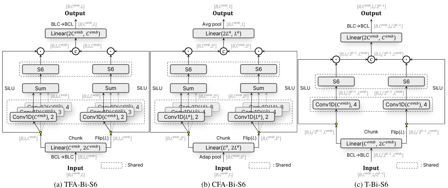
Figure 3. Diagrams of the Feature aggregated Bi-S6 block design. (a) TFA-Bi-S6 model. (b) CFA-Bi-S6 model. (c) T-Bi-S6 mode.
图 3: 特征聚合 Bi-S6 块设计示意图。(a) TFA-Bi-S6 模型。(b) CFA-Bi-S6 模型。(c) T-Bi-S6 模型。
Dual Bi-S6 Structure The Dual Bi-S6 structure is a novel component of our proposed architecture, designed to enhance the modeling of s patio temporal dependencies by processing features along both the temporal and channel dimensions. This dual-path approach ensures that the model can capture and integrate the rich contextual information present in video sequences, thereby improving the accuracy of TAL.
双Bi-S6结构
双Bi-S6结构是我们提出架构中的创新组件,旨在通过同时处理时间和通道维度的特征来增强时空依赖建模。这种双路径方法确保模型能够捕捉并整合视频序列中丰富的上下文信息,从而提升TAL (Temporal Action Localization) 的准确性。
As shown in Figure 2b, the Dual Bi-S6 structure consists of two parallel paths: the TFA-Bi-S6 and the CFA-Bi-S6. Each path processes the input sequence differently to extract complementary information. The TFA-Bi-S6 reflects temporal dynamics within the video sequence, providing a detailed temporal analysis of the input. Simultaneously, the CFA-Bi-S6 captures the interactions between different s patio temporal features, and its output is then scaled using a sigmoid function to transform the values into a range suitable for modulation.
如图 2b 所示,Dual Bi-S6 结构由两条并行路径组成:TFA-Bi-S6 和 CFA-Bi-S6。每条路径以不同方式处理输入序列以提取互补信息。TFA-Bi-S6 反映视频序列中的时间动态,提供对输入的详细时间分析。同时,CFA-Bi-S6 捕获不同时空特征之间的交互作用,其输出随后通过 sigmoid 函数进行缩放,将数值转换为适合调制的范围。
After processing the input through both paths, the outputs of the TFA-Bi-S6 and CFA-Bi-S6 are combined using point-wise multiplication. This fusion step integrates the temporal dependencies captured by the TFA-Bi-S6 with the channel-wise dependencies modeled by the CFA-Bi-S6. The point-wise multiplication ensures that the combined features reflect both types of dependencies, with the TFA-Bi-S6 handling global dependencies between clips and the CFA-Bi-S6 addressing local dependencies between s patio temporal features within clips. The design intention behind this structure is to leverage the strengths of both paths: the TFA-Bi-S6 captures temporal dependencies and dynamics, while the CFA-Bi-S6 emphasizes the relationships between spatiotemporal features. By scaling the output of the CFA-Bi-S6 and multiplying it with the TFA-Bi-S6 output, the model effectively combines temporal analysis with channel-wise context, leading to a more comprehensive understanding of the video.
经过两条路径处理输入后,TFA-Bi-S6和CFA-Bi-S6的输出通过逐点乘法进行融合。这一融合步骤将TFA-Bi-S6捕捉的时间依赖性与CFA-Bi-S6建模的通道间依赖性相结合。逐点乘法确保组合特征能同时反映两种依赖关系:TFA-Bi-S6处理片段间的全局依赖性,CFA-Bi-S6则处理片段内时空特征间的局部依赖性。该结构的设计意图是发挥两条路径的优势:TFA-Bi-S6捕获时间依赖性和动态变化,而CFA-Bi-S6强调时空特征间的关系。通过缩放CFA-Bi-S6输出并与TFA-Bi-S6输出相乘,模型有效地将时间分析与通道上下文结合,从而实现对视频更全面的理解。
Recurrent Mechanism This mechanism, integrated with our Stem module in the Backbone, enhances the accuracy of temporal context modeling by leveraging the efficiency and precision of state space models. As shown in Figure 2b, the process begins by passing the input sequence through the Stem module to capture initial temporal dependencies. The output is combined with the original input sequence and reprocessed by the Stem module, repeating this process $r$ times. Each iteration refines the temporal dependencies further, enhancing the model's ability to capture long-range dependencies and intricate temporal patterns. This recurrent mechanism provides a robust framework for refining temporal context, allowing the model to improve its understanding of temporal dependencies dynamically.
循环机制
该机制与主干网络中的Stem模块结合,通过利用状态空间模型的效率和精度,提升了时序上下文建模的准确性。如图2b所示,该过程首先将输入序列通过Stem模块以捕获初始时序依赖关系。输出结果与原始输入序列结合后,由Stem模块重新处理,此过程重复$r$次。每次迭代都会进一步优化时序依赖关系,增强模型捕捉长程依赖和复杂时序模式的能力。这种循环机制为时序上下文优化提供了鲁棒框架,使模型能够动态提升对时序依赖关系的理解。
The effectiveness of this recurrent mechanism in speech separation tasks highlights its potential for TAL tasks as well. In speech separation, recurrent mechanisms have proven to excel in capturing long-range dependencies and intricate temporal patterns [6, 14]. This iterative refinement process, which involves passing the input sequence through a module multiple times to capture and refine temporal dependencies, allows models to handle complex long-range dependencies with greater precision. Such capabilities are directly applicable to TAL tasks, where identifying precise segments within a video also requires understanding temporal dependencies over extended periods.
这种循环机制在语音分离任务中的有效性,也凸显了其在时序动作定位(TAL)任务中的潜力。在语音分离领域,循环机制已被证明擅长捕捉长距离依赖关系和复杂的时间模式 [6, 14]。这种通过多次将输入序列传递至模块以捕获并优化时间依赖关系的迭代细化过程,使模型能够更精准地处理复杂的长距离依赖。此类能力直接适用于时序动作定位任务——在视频中精确定位动作片段同样需要理解长时间跨度的时间依赖关系。
| Base | System | @.3 | @.4 | @.5 | @.6 | @.7 | Avg | Base | System | @.5 | @.75 | @.95 | Avg |
|---|---|---|---|---|---|---|---|---|---|---|---|---|---|
| CNN | CDC [29] | 40.1 | 29.4 | 23.3 | 13.1 | 7.9 | 22.8 | CNN | BSN [19] | 46.5 | 30.0 | 8.0 | 30.0 |
| CNN | TAL-Net [5] | 53.2 | 48.5 | 42.8 | 33.8 | 20.8 | 39.8 | DCAN [8] | 51.8 | 36.0 | 9.5 | 35.4 | |
| CNN | PBRNet [20] | 58.5 | 54.6 | 51.3 | 41.8 | 29.5 | 47.1 | RNN | DeepAct [30] | 37.8 | 24.8 | 10.0 | 24.0 |
| RNN | AS [1] | 51.8 | 42.4 | 30.8 | 20.2 | 11.1 | 31.3 | GCN | G-TAD [36] | 50.4 | 34.6 | 9.0 | 34.1 |
| RNN | RCL [34] | 70.1 | 62.3 | 52.9 | 42.7 | 30.7 | 51.7 | AVFusion [3] | 54.3 | 37.7 | 8.9 | 36.8 | |
| GCN | G-TAD [36] | 66.4 | 60.4 | 51.6 | 37.6 | 22.9 | 47.8 | Transformer | ActionFormer [42] | 54.7 | 37.8 | 8.4 | 36.6 |
| Transformer | TallFormer [9] | 76.0 | 71.5 | 63.2 | 50.9 | 34.5 | 59.2 | TriDet [28] | 54.7 | 38.0 | 8.4 | 36.8 | |
| Transformer | ActionFormer [42] | 82.1 | 77.8 | 71.0 | 59.4 | 43.9 | 66.8 | TCANet [27] | 54.3 | 39.1 | 8.4 | 37.6 | |
| Transformer | TriDet [28] | 83.6 | 80.1 | 72.9 | 62.4 | 47.4 | 69.3 | AdaTAD [21] | 61.7 | 43.4 | 10.9 | 41.9 | |
| S6 | ActionMamba[7] | 86.9 | 83.1 | 76.9 | 65.1 | 50.8 | 72.7 | S6 | ActionMamba[7] | 62.4 | 43.5 | 10.2 | 42.0 |
| Ours | 88.7 | 84.6 | 78.2 | 66.6 | 51.9 | 74.2 | Ours | 64.1 | 44.0 | 10.6 | 42.9 | ||
| (a) | (b) |
| Base | System | mAP (%) | @.95 | Base | System | mAP (%) | ||||||
|---|---|---|---|---|---|---|---|---|---|---|---|---|
| CNN | DBG [18] | @.5 10.7 | @.75 6.4 | 2.5 | Avg 6.8 | CNN | DyFADet [39] | @.5 64.0 | @.75 44.8 | @.95 | Avg 44.3 | |
| GCN | G-TAD [36] | 13.7 | 8.8 | 3.1 | 9.1 | Transformer | TadTR [22] | 47.1 | 32.1 | 14.1 10.9 | 32.1 | |
| Transformer | VideoMAE-v2[33] | 29.1 | 17.7 | 5.1 | 18.2 | TriDet [28] | 62.4 | 44.1 | 13.1 | 43.1 | ||
| S6 | ActionMamba [7] | 45.4 | 28.8 | 6.8 | 29.0 | S6 | ActionMamba [7] | 64.0 | 45.7 | 13.3 | 44.6 | |
| Ours | 46.4 | 29.5 | 7.6 | 29.6 | Ours | 66.4 | 47.2 | 14.3 | 45.8 | |||
| (c) | (d) |
4. Experiments
4. 实验
We provide a comprehensive evaluation of our TAL method through extensive experiments. We demonstrate its effectiveness using various benchmark datasets and conduct ablation studies to assess the impact of various components of our proposed approach.
我们通过大量实验对TAL方法进行了全面评估。使用多种基准数据集验证了其有效性,并通过消融实验评估了所提方法各组成部分的影响。
4.1. Evaluation on Benchmarks
4.1. 基准测试评估
To evaluate the effectiveness of the proposed method for TAL, we utilized the benchmark datasets THUMOS-14 [15], Activity Net [4], FineAction [23], and HACS [43]. Detailed descriptions of each benchmark can be found in Appendix B.
为评估所提时序动作定位(TAL)方法的有效性,我们采用了THUMOS-14 [15]、ActivityNet [4]、FineAction [23]和HACS [43]基准数据集。各基准的详细说明见附录B。
Table 1a presents experimental results on THUMOS-14. We compared our method with various approaches, including CNNs, RNNs, GCNs, Transformers-based, and the latest SOTA S6-based model. Our method achieved an average mAP of $74.2%$ , surpassing the previous SOTA by $1.5%$ . In Table 1b, we summarize our performance on Activity Net. Despite its larger scale and variety of classes, which generally result in lower scores, our method achieved an average mAP of $42.9%$ , surpassing the previous SOTA by $0.9%$
表 1a 展示了在 THUMOS-14 上的实验结果。我们将本方法与多种方法进行了对比,包括 CNN、RNN、GCN、基于 Transformer 的方法以及最新的基于 S6 的 SOTA 模型。本方法的平均 mAP 达到 $74.2%$,比之前的 SOTA 高出 $1.5%$。表 1b 总结了我们在 Activity Net 上的表现。尽管该数据集规模更大、类别更多样化(通常会导致得分降低),但本方法的平均 mAP 仍达到 $42.9%$,比之前的 SOTA 高出 $0.9%$。
The outcomes on FineAction are presented in Table 1c. This benchmark, being relatively new, lacked RNN-based studies for comparison. Therefore, we included studies utilizing CNN, GCN, Transformer, and S6 models. FineAction's high class variety relative to its size makes it particularly challenging, generally resulting in lower mAP scores. Nonetheless, our approach achieved an average mAP Oof $29.6%$ ,which is $0.6%$ higher than the previous SOTA. Finally, Table 1d displays our experimental performance on HACS. Most studies focused on Transformer-based approaches due to the dataset's large scale. Despite this, our proposed method achieved an average mAP of $45.8%$ ,exceeding the previous SOTA by $1.2%$
FineAction 上的结果展示在表 1c 中。由于该基准相对较新,缺乏基于 RNN 的研究进行比较,因此我们纳入了使用 CNN、GCN、Transformer 和 S6 模型的研究。FineAction 的高类别多样性相对于其规模使其特别具有挑战性,通常会导致较低的 mAP 分数。尽管如此,我们的方法实现了平均 mAP 为 $29.6%$,比之前的 SOTA 高出 $0.6%$。最后,表 1d 展示了我们在 HACS 上的实验性能。由于数据集规模庞大,大多数研究集中在基于 Transformer 的方法上。尽管如此,我们提出的方法实现了平均 mAP 为 $45.8%$,比之前的 SOTA 高出 $1.2%$。
4.2. Ablation Studies
4.2. 消融研究
Stem module structure and Block quantities We investigated the impact of varying the structure of the Stem module and the number of blocks in the Embedding, Stem, and Branch modules to understand their effect on performance.
主干模块结构与块数量 我们研究了改变主干模块结构以及嵌入、主干和分支模块中块数量对性能的影响。
The results, presented in Table 2a, demonstrate the superiority of the Dual structure in the Stem module, which utilizes both temporal and channel blocks, consistently outperforming the Single structure that only uses the temporal block. This finding suggests that addressing both temporal and channel-wise dependencies provides a more comprehensive understanding for TAL. Additionally, using a single block in each module often yielded better performance than multiple blocks, indicating that simpler, less complex model structures help prevent over fitting and effectively capture essential s patio temporal features. Notably, omitting the Stem module( $\mathit{\Delta}{\mathit{B}_{s}}=0$ ) results in a significant performance drop, highlighting its importance in sequence interpretation.
表 2a 中的结果表明,在 Stem 模块中采用同时使用时序块和通道块的双重结构 (Dual structure) 始终优于仅使用时序块的单一结构 (Single structure)。这一发现表明,同时处理时序和通道维度的依赖关系能为时序动作定位 (TAL) 提供更全面的理解。此外,每个模块使用单一区块通常比使用多个区块表现更好,说明更简单、复杂度较低的模型结构有助于防止过拟合,并能有效捕捉关键的时空特征。值得注意的是,省略 Stem 模块 ( $\mathit{\Delta}{\mathit{B}_{s}}=0$ ) 会导致性能显著下降,这凸显了该模块在序列解析中的重要性。
Kernel sizes and Aggregation methods We evaluated the performance impact of different kernel size combinations for TFA-Bi-S6 and CFA-Bi-S6 blocks and various aggregation methods using the Dual structure. This analysis, detailed in Table 2b, explores how different configurations influence the model's ability to capture temporal and channel-wise local context.
核大小与聚合方法
我们评估了TFA-Bi-S6和CFA-Bi-S6模块中不同核大小组合以及使用Dual结构的多种聚合方法对性能的影响。如表2b所示,该分析探讨了不同配置如何影响模型捕获时间和通道局部上下文的能力。
Table 2. Ablation studies on the proposed methods. (a) Performance comparison with varying numbers of blocks in the Embedding, Stem, and Branch modules $(B_{e},B_{s},B_{b})$ and different structures (Structure) using only single Conv1D layer without Feature Aggregation. In this context, “Single” refers to using only the temporal block in the Stem module, while “Dual" refers to using both the temporal and channel blocks in the Stem module. (b) Performance comparison with different kernel size combinations for TFA-Bi-S6 and CFA-Bi-S6 blocks $\overset{\prime}{K}{T F A}$ and $K_{C F A}$ ) and different aggregation methods (Aggregate) using the Dual structure. (c) Performance comparison with varying iterations $(r)$ of applying residual connections in the recurrent Dual S6 structure in the Stem module and different numbers of blocks in the Stemmodule $(B_{s})$ , with both Dual structure and Feature Aggregation applied. All results are from the THUMOS-14 dataset.
表 2. 所提方法的消融研究。(a) 在仅使用单层Conv1D且无特征聚合的情况下,Embedding、Stem和Branch模块中不同块数$(B_{e},B_{s},B_{b})$与不同结构(Structure)的性能对比。此处的"Single"指仅在Stem模块中使用时序块,而"Dual"指同时使用时序块和通道块。(b) 采用Dual结构时,TFA-Bi-S6和CFA-Bi-S6块的不同核尺寸组合($\overset{\prime}{K}{T F A}$和$K_{C F A}$)与不同聚合方法(Aggregate)的性能对比。(c) 在同时应用Dual结构和特征聚合的情况下,Stem模块中循环Dual S6结构应用残差连接的不同迭代次数$(r)$与Stem模块中不同块数$(B_{s})$的性能对比。所有结果均来自THUMOS-14数据集。
| Structure(Be,Bs,Bb) | Params (M) | Avg mAP (%) | KTFA | KcFA Aggregate | Params (M) (%) | Bs | r | Params (M) | Avg mAP (%) |
|---|---|---|---|---|---|---|---|---|---|
| Single | (1,0,1) | 16.0 | 69.4 | X | X | Sum | 20.5 | 72.1 | 1 |
| (1,1,1) | 18.8 | 72.2 | (4) | X | Sum | 21.6 | 72.6 | ||
| (2,1,1) | 19.6 | 72.0 | X | (4) | Sum | 20.6 | 72.3 | ||
| (1,2,1) | 21.6 | 71.7 | (4) | (4) | Sum | 21.7 | 72.8 | ||
| (1,1,2) | 33.0 | 71.0 | (2,4) | (4) | Sum | 22.1 | 73.0 | ||
| (2,2,1) | 22.5 | 71.8 | (4) | (2,4) | Sum | 21.7 | 72.9 | ||
| (2,1,2) | 33.8 | 71.1 | (2,4) | (2,4) | Sum | 22.2 | 73.1 | 2 | |
| (1,2,2) | 35.9 | 71.3 | (2,3,4) | (2,3,4) | Sum | 23.0 | 73.4 | ||
| (2,2,2) | 36.6 | 71.5 | (2,3,4,8) | (2,3,4,8) | Sum | 25.2 | 73.2 | ||
| (1,4,1) | 27.3 | 71.3 | (2,4,8) | (2,3,4) | Sum | 24.3 | 73.4 | 4 | |
| (1,8,1) | 38.6 | 70.7 | (2,3,4) | (2,4,8) | Sum | 23.1 | 73.5 | ||
| Dual | (1,1,1) | 21.7 | 72.8 72.5 | (2,3,4) (2,4,8) | (2,4,8) (2,4,8) | Concat | 31.6 24.5 | 72.8 73.4 | |
| (1,2,1) (a) | 28.5 | Sum (b) | 8 |
The results show that using multiple kernel sizes for Conv1D layers in both TFA-Bi-S6 and CFA-Bi-S6 blocks improves performance, demonstrating the benefit of capturing a diverse range of local contexts at multiple scales for TAL. However, configurations with four or more kernel sizes per block resulted in decreased performance, likely due to over fitting, as the increased model complexity led to learning noise and less relevant patterns.
结果表明,在TFA-Bi-S6和CFA-Bi-S6模块中为Conv1D层使用多核尺寸能提升性能,这证明了为时序动作定位(TAL)任务捕获多尺度多样化局部上下文的有效性。然而,当每个模块采用四个及以上核尺寸时,性能反而下降,这可能是由于模型复杂度增加导致过拟合,使其学习了噪声和无关模式。
The absence of Conv1D layers led to reduced performance, underscoring the importance of capturing temporal and channel-wise local context through these layers. Furthermore, the Sum aggregation method outperformed the Concat method, indicating that summing feature maps effectively integrates information across different scales without adding excessive complexity.
移除Conv1D层会导致性能下降,这凸显了通过这些层捕捉时间和通道局部上下文的重要性。此外,Sum聚合方法优于Concat方法,表明求和特征图能有效整合不同尺度的信息,同时避免引入过多复杂度。
Recurrent mechanism iterations We examined the impact of varying the number of iterations $r$ in the recurrent mechanism, along with the Dual structure and Feature $A g$ gregation. This analysis, detailed in Table 2c, assesses how iterative refinement of temporal dependencies affects model performance compared to increasing the number of Stem blocks $(B_{s})$
循环机制迭代
我们研究了在循环机制中改变迭代次数 $r$ 的影响,同时结合了双重结构 (Dual structure) 和特征聚合 (Feature Aggregation)。如表 2c 所示,该分析评估了与增加 Stem 块数量 $(B_{s})$ 相比,时间依赖性的迭代优化如何影响模型性能。
The results show that increasing the number of recurrent iterations $r$ generally improves performance up to a certain point. Beyond this point, however, additional iterations resulted in a slight performance drop, likely due to an imbalance in temporal dependency. This suggests that there is an optimal number of iterations after which the benefits begin to diminish. In contrast, increasing the number of Stem blocks $(B_{s})$ while keeping $r$ fixed at 1 led to a decrease in performance, indicating that simply adding more Stem blocks is not effective for improving TAL.
结果表明,增加循环迭代次数 $r$ 通常能在一定程度上提升性能。然而超过该临界点后,继续增加迭代次数会导致性能轻微下降,这可能是由于时序依赖性失衡所致。这说明存在一个最优迭代次数,超过该值后收益开始递减。相比之下,在固定 $r=1$ 的情况下增加 Stem 模块数量 $(B_{s})$ 会导致性能下降,表明单纯增加 Stem 模块并不能有效提升 TAL。
This comparison shows that adopting a recurrent approach, with $B_{s}$ set to 1 and increasing $r$ , is more efficient and effective than stacking additional blocks. The recurrent mechanism improves temporal precision and long-range dependency modeling while optimizing memory usage, crucial for accurately understanding extended actions in video sequences and boosting performance, making it a practical strategy for TAL tasks using the S6-based model.
这一对比表明,采用循环方法(将 $B_{s}$ 设为1并逐步增加 $r$)比堆叠额外模块更高效且有效。循环机制提升了时序精度和长程依赖建模能力,同时优化了内存使用——这对准确理解视频序列中的长时动作及提升性能至关重要,使其成为基于S6模型的时间动作定位(TAL)任务的实用策略。
5. Conclusion
5. 结论
In this paper, we introduced a novel architecture leveraging S6 to provide effective solutions for TAL tasks based on insights from previous studies. By integrating the Feature Aggregated Bi-S6 block and the Dual Bi-S6 structure, our approach captures multi-scale temporal and channelwise dependencies. The recurrent mechanism further refines temporal context modeling, enhancing performance without increasing parameter complexity. Consequently, our approach achieves state-of-the-art results on various benchmark datasets, with average mAP scores of $74.2%$ on THUMOS14, $42.9%$ on Activity Net, $29.6%$ on FineAction, and $45.8%$ on HACS. Additionally, ablation studies confirm the advantages of our design, demonstrating that the Dual structure in the Stem module outperforms the Single structure, the recurrent mechanism is more effective than merely stacking additional blocks, and Temporal Aggregation further boosts performance. These findings pave the way for future research to further explore the potential of state space models in TAL tasks.
本文提出了一种基于S6的新型架构,通过整合特征聚合双向S6模块(FAB)和双路双向S6结构,有效解决了时序动作定位(TAL)任务中的多尺度时序与通道依赖问题。循环机制进一步优化了时序上下文建模,在不增加参数复杂度的前提下提升了性能。实验表明,该方法在THUMOS14(74.2% mAP)、ActivityNet(42.9%)、FineAction(29.6%)和HACS(45.8%)等基准数据集上达到了最先进水平。消融研究证实:主干模块中的双路结构优于单路结构,循环机制比单纯堆叠模块更有效,时序聚合能进一步提升性能。这些发现为未来探索状态空间模型在TAL任务中的潜力奠定了基础。
A. Example of Pretrained Video Encoder Extracting S patio temporal Features from Each Clip
A. 预训练视频编码器从每个片段提取时空特征的示例
To understand the design intention of the Dual Bi-S6 structure, it is crucial to explain how the Pretrained video encoder extracts s patio temporal features from each clip, clarifying the information contained in the sequence.
为了理解Dual Bi-S6结构的设计意图,关键在于说明预训练视频编码器如何从每个片段中提取时空特征,从而阐明序列中包含的信息。
For instance, when processing the THUMOS dataset using the same Pretrained video encoder as Action Mamba, we start with RGB videos at 30 fps and a spatial resolutionof $224\mathrm{x}224$ . We segment 16 frames into a single clip, setting a frame interval of 4 (stride $_{:=4}$ )between clips, yielding multiple clips from each video, each clip measuring [3, 16, 224, 224]. Within each frame, patches of size 14x14 are generated, producing 256 patch tokens per frame. Each patch token, representing spatial information and RGB channels, is flattened to a dimension of [256, 588]. These spatial tokens are projected to a channel size of 3200, forming patch embedding tokens with dimensions [16, 256, 3200]. Adding 3D sine-cosine positional embeddings to both the patch and frame dimensions, and then flattening these dimensions, results in position-embedded tokens with dimensions [4096, 3200]. Next, a proportion $\rho$ of tokens is masked, and the channels are projected to 3200, followed by multihead self-attention and a feed forward layer with a hidden channel size of 12800, repeated 48 times to incorporate spatio temporal context, resulting in contextual embedded tokens with dimensions $[4096(1-\rho),32\$ 00]. Finally, multi-head self-attention and mean pooling are applied along the token dimension to produce an encoded feature vector with dimensions $[1,3200]$ for each clip. This process is repeated for all clips, stacking the encoded feature vectors sequentially over time to generate the sequence data, excluding the first and last two clips, which may lack video information, as shown in Figure 4.
例如,在使用与Action Mamba相同的预训练视频编码器处理THUMOS数据集时,我们从30 fps、空间分辨率为$224\mathrm{x}224$的RGB视频开始。将16帧分割为一个片段,设置片段间帧间隔为4(步长$_{:=4}$),从每个视频中生成多个片段,每个片段尺寸为[3, 16, 224, 224]。在每帧中生成14x14的块(patch),每帧产生256个块token。每个代表空间信息和RGB通道的块token被展平为[256, 588]的维度。这些空间token被投影到3200的通道大小,形成维度为[16, 256, 3200]的块嵌入token。向块和帧维度添加3D正弦-余弦位置嵌入后展平这些维度,得到维度为[4096, 3200]的位置嵌入token。接着按比例$\rho$掩码部分token,将通道投影到3200,随后通过48次多头自注意力层和隐藏通道大小为12800的前馈层来融入时空上下文,最终得到维度为$[4096(1-\rho),32\$00]的上下文嵌入token。最后沿token维度应用多头自注意力和均值池化,为每个片段生成维度$[1,3200]$的编码特征向量。对所有片段重复此过程,按时间顺序堆叠编码特征向量以生成序列数据(排除可能缺少视频信息的首尾两个片段),如图4所示。
B. Benchmark Datasets for Temporal Action Localization
B. 时序动作定位基准数据集
To provide a comprehensive evaluation of TAL methods, we employ several benchmark datasets that vary in size, complexity, and focus. Here, we describe the key characteristics and evaluation metrics of the datasets utilized in this study:
为了全面评估TAL方法,我们采用了多个在规模、复杂度和关注点上各异的基准数据集。以下描述本研究所用数据集的关键特征和评估指标:
THUMOS-14: This large-scale dataset is specifically designed for video action recognition and includes detailed temporal frame index annotations for 20 action classes. The primary evaluation metric for THUMOS-14 is mean Average Precision (mAP), which is calculated at various temporal Intersection over Union (tIoU) thresholds of 0.3, 0.4, 0.5, 0.6, and 0.7. This allows for a thorough assessment of the model's performance across different levels of temporal precision.
THUMOS-14: 该大型数据集专为视频动作识别设计,包含20个动作类别的详细时间帧索引标注。THUMOS-14的主要评估指标是平均精度均值(mAP),通过在0.3、0.4、0.5、0.6和0.7等多个时间交并比(tIoU)阈值下计算得出,从而全面评估模型在不同时间精度级别上的性能。
Activity Net: Significantly larger and more complex than THUMOS-14, Activity Net comprises approximately 20,000 videos spanning 200 action classes. The diverse range of classes in Activity Net presents a more challenging scenario for TAL models. The mAP evaluation metric is also employed here, with tIoU thresholds set at 0.5, 0.75, and 0.95, providing a stringent test for action localization performance.
Activity Net:比THUMOS-14数据集规模更大、复杂度更高,包含约20,000个视频,涵盖200个动作类别。其多样化的类别为时序动作定位(TAL)模型带来了更大挑战。该数据集同样采用mAP(平均精度均值)评估指标,并设置0.5、0.75和0.95三个tIoU(时序交并比)阈值,为动作定位性能提供严格测试标准。
FineAction: Consisting of around 16,000 videos featuring 106 action classes, FineAction emphasizes everyday activities and sports. The high variety of classes relative to its size makes it a particularly challenging dataset. Evaluation methods are akin to those used for Activity Net, utilizing mAP scores at multiple tIoU thresholds.
FineAction:该数据集包含约16,000段视频,涵盖106个动作类别,重点关注日常活动和体育运动。其类别数量与数据规模的高比例使其成为极具挑战性的基准数据集。评估方式与Activity Net类似,采用多组tIoU阈值下的mAP分数进行衡量。
HACS (Human Action Clips and Segments): This extensive dataset includes approximately 50,000 videos covering 200 action classes, primarily capturing various actions from everyday life. Evaluation of the HACS dataset is conducted using the same methodology as Activity Net, ensuring a consistent benchmark for comparing TAL model performance across different datasets.
HACS (Human Action Clips and Segments): 该数据集包含约5万段视频,涵盖200个动作类别,主要记录日常生活中的各类行为。HACS数据集的评估采用与Activity Net相同的方法论,确保跨数据集时态动作定位(TAL)模型性能对比的基准一致性。
These detailed descriptions of the datasets underscore the diverse and comprehensive nature of the benchmarks used in this study, providing a robust framework for evaluating the effectiveness of TAL methods.
这些数据集的详细描述凸显了本研究所用基准的多样性和全面性,为评估TAL方法的有效性提供了稳健框架。