SHARPNESS-AWARE MINIMIZATION FOR EFFICIENTLY IMPROVING GENERALIZATION
基于锐度感知最小化的高效泛化提升方法
ABSTRACT
摘要
In today’s heavily over parameterized models, the value of the training loss provides few guarantees on model generalization ability. Indeed, optimizing only the training loss value, as is commonly done, can easily lead to suboptimal model quality. Motivated by prior work connecting the geometry of the loss landscape and generalization, we introduce a novel, effective procedure for instead simultaneously minimizing loss value and loss sharpness. In particular, our procedure, Sharpness-Aware Minimization (SAM), seeks parameters that lie in neighborhoods having uniformly low loss; this formulation results in a minmax optimization problem on which gradient descent can be performed efficiently. We present empirical results showing that SAM improves model genera liz ation across a variety of benchmark datasets (e.g., CIFAR ${10,100}$ , ImageNet, finetuning tasks) and models, yielding novel state-of-the-art performance for several. Additionally, we find that SAM natively provides robustness to label noise on par with that provided by state-of-the-art procedures that specifically target learning with noisy labels. We open source our code at https: //github.com/google-research/sam.
在当今高度过参数化的模型中,训练损失值对模型泛化能力的保证十分有限。事实上,仅优化训练损失值(这是常见做法)很容易导致模型质量欠佳。受先前关于损失函数几何形状与泛化能力关联研究的启发,我们提出了一种新颖有效的方法,可同时最小化损失值和损失锐度。具体而言,我们的锐度感知最小化(Sharpness-Aware Minimization,SAM)方法会寻找处于均匀低损失邻域的参数;该方案形成了一个可通过梯度下降高效求解的极小极大优化问题。实验结果表明,SAM在多种基准数据集(如CIFAR ${10,100}$、ImageNet、微调任务)和模型上均提升了泛化能力,并在多项任务中创造了最新最优性能。此外,我们发现SAM天然具备与专门针对噪声标签学习的最先进方法相当的标签噪声鲁棒性。代码已开源:https://github.com/google-research/sam。
1 INTRODUCTION
1 引言
Modern machine learning’s success in achieving ever better performance on a wide range of tasks has relied in significant part on ever heavier over parameter iz ation, in conjunction with developing ever more effective training algorithms that are able to find parameters that generalize well. Indeed, many modern neural networks can easily memorize the training data and have the capacity to readily overfit (Zhang et al., 2016). Such heavy over parameter iz ation is currently required to achieve stateof-the-art results in a variety of domains (Tan & Le, 2019; Kolesnikov et al., 2020; Huang et al., 2018). In turn, it is essential that such models be trained using procedures that ensure that the parameters actually selected do in fact generalize beyond the training set.
现代机器学习之所以能在广泛任务上取得越来越好的性能,很大程度上依赖于日益严重的过参数化(overparameterization),同时配合开发出更高效的训练算法,这些算法能够找到具有良好泛化能力的参数。事实上,许多现代神经网络可以轻松记住训练数据,并具备容易过拟合的能力 (Zhang et al., 2016)。目前要在多个领域取得最先进的结果,这种严重的过参数化是必需的 (Tan & Le, 2019; Kolesnikov et al., 2020; Huang et al., 2018)。因此,必须通过训练流程确保实际选择的参数确实能够泛化到训练集之外。
Unfortunately, simply minimizing commonly used loss functions (e.g., cross-entropy) on the training set is typically not sufficient to achieve satisfactory generalization. The training loss landscapes of today’s models are commonly complex and non-convex, with a multiplicity of local and global minima, and with different global minima yielding models with different generalization abilities (Shirish Keskar et al., 2016). As a result, the choice of optimizer (and associated optimizer settings) from among the many available (e.g., stochastic gradient descent (Nesterov, 1983), Adam (Kingma & Ba, 2014), RMSProp (Hinton et al.), and others (Duchi et al., 2011; Dozat, 2016; Martens & Grosse, 2015)) has become an important design choice, though understanding of its relationship to model generalization remains nascent (Shirish Keskar et al., 2016; Wilson et al., 2017; Shirish Keskar & Socher, 2017; Agarwal et al., 2020; Jacot et al., 2018). Relatedly, a panoply of methods for modifying the training process have been proposed, including dropout (Srivastava et al., 2014), batch normalization (Ioffe & Szegedy, 2015), stochastic depth (Huang et al., 2016), data augmentation (Cubuk et al., 2018), and mixed sample augmentations (Zhang et al., 2017; Harris et al., 2020).
遗憾的是,仅通过在训练集上最小化常用损失函数(如交叉熵)通常不足以获得令人满意的泛化效果。当今模型的训练损失曲面往往复杂且非凸,存在大量局部极小值和全局极小值,而不同的全局极小值会产生具有不同泛化能力的模型(Shirish Keskar等人,2016)。因此,从众多可选的优化器(如随机梯度下降(Nesterov,1983)、Adam(Kingma & Ba,2014)、RMSProp(Hinton等人)及其他(Duchi等人,2011;Dozat,2016;Martens & Grosse,2015))中选择优化器(及相关设置)已成为关键设计决策,尽管对其与模型泛化关系的理解仍处于初级阶段(Shirish Keskar等人,2016;Wilson等人,2017;Shirish Keskar & Socher,2017;Agarwal等人,2020;Jacot等人,2018)。相关地,研究者们提出了多种改进训练过程的方法,包括dropout(Srivastava等人,2014)、批归一化(Ioffe & Szegedy,2015)、随机深度(Huang等人,2016)、数据增强(Cubuk等人,2018)以及混合样本增强(Zhang等人,2017;Harris等人,2020)。
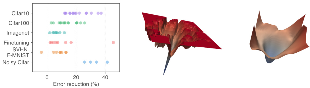
Figure 1: (left) Error rate reduction obtained by switching to SAM. Each point is a different dataset / model / data augmentation. (middle) A sharp minimum to which a ResNet trained with SGD converged. (right) A wide minimum to which the same ResNet trained with SAM converged.
图 1: (左) 改用SAM (Sharpness-Aware Minimization) 获得的错误率降低。每个点代表不同的数据集/模型/数据增强方案。(中) 使用SGD训练的ResNet收敛到的尖锐最小值。(右) 使用SAM训练的相同ResNet收敛到的平坦最小值。
The connection between the geometry of the loss landscape—in particular, the flatness of minima— and generalization has been studied extensively from both theoretical and empirical perspectives (Shirish Keskar et al., 2016; Dziugaite & Roy, 2017; Jiang et al., 2019). While this connection has held the promise of enabling new approaches to model training that yield better generalization, practical efficient algorithms that specifically seek out flatter minima and furthermore effectively improve generalization on a range of state-of-the-art models have thus far been elusive (e.g., see (Chaudhari et al., 2016; Izmailov et al., 2018); we include a more detailed discussion of prior work in Section 5).
损失函数景观的几何特性(尤其是极小值的平坦度)与泛化能力之间的关联,已从理论和实证角度得到广泛研究(Shirish Keskar等,2016;Dziugaite & Roy,2017;Jiang等,2019)。尽管这种关联为开发具有更好泛化性能的模型训练方法提供了可能,但迄今为止,能够专门寻找更平坦极小值并有效提升各类前沿模型泛化能力的实用高效算法仍难以实现(例如参见Chaudhari等,2016;Izmailov等,2018;我们将在第5节详细讨论先前工作)。
We present here a new efficient, scalable, and effective approach to improving model generalization ability that directly leverages the geometry of the loss landscape and its connection to generalization, and is powerfully complementary to existing techniques. In particular, we make the following contributions:
我们在此提出一种高效、可扩展且有效的新方法,通过直接利用损失函数曲面的几何特性及其与泛化能力的关联来提升模型泛化性能,该方法与现有技术形成有力互补。具体贡献如下:
Section 2 below derives the SAM procedure and presents the resulting algorithm in full detail. Section 3 evaluates SAM empirically, and Section 4 further analyzes the connection between loss sharpness and generalization through the lens of SAM. Finally, we conclude with an overview of related work and a discussion of conclusions and future work in Sections 5 and 6, respectively.
以下第2节推导了SAM (Sharpness-Aware Minimization) 方法并完整呈现算法细节。第3节通过实验评估SAM的性能,第4节从SAM角度进一步分析损失函数锐度与泛化能力的关系。最后,第5节概述相关工作,第6节分别讨论结论与未来研究方向。
2 SHARPNESS-AWARE MINIMIZATION (SAM)
2 锐度感知最小化 (SAM)
Motivated by the connection between sharpness of the loss landscape and generalization, we propose a different approach: rather than seeking out parameter values $\mathbf{\nabla}{\mathbf{\overrightarrow{\mathbf{\vert~\mathbf{\nabla~}~}}}}$ that simply have low training loss value $L_{\mathcal{S}}({\boldsymbol{\mathbf{\mathit{w}}}})$ , we seek out parameter values whose entire neighborhoods have uniformly low training loss value (equivalently, neighborhoods having both low loss and low curvature). The following theorem illustrates the motivation for this approach by bounding generalization ability in terms of neighborhood-wise training loss (full theorem statement and proof in Appendix A):
受损失函数曲面锐度与泛化能力之间关联的启发,我们提出了一种新方法:不同于仅寻找训练损失值 $L_{\mathcal{S}}({\boldsymbol{\mathbf{\mathit{w}}}})$ 较低的参数值 $\mathbf{\nabla}_{\mathbf{\overrightarrow{\mathbf{\vert~\mathbf{\nabla~}~}}}}$ ,我们致力于寻找其整个邻域内训练损失值均保持较低水平的参数值(即同时具备低损失与低曲率的邻域)。以下定理通过邻域训练损失对泛化能力进行界定,阐明了该方法的理论依据(完整定理表述及证明见附录A):
Theorem (stated informally) 1. For any $\rho>0$ , with high probability over training set $s$ generated from distribution $\mathcal{D}$ ,
定理 (非正式表述) 1. 对于任意 $\rho>0$,在从分布 $\mathcal{D}$ 生成的训练集 $s$ 上,以高概率成立。
$$
L_{\mathcal{D}}(\pmb{w})\leq\operatorname*{max}{|\pmb{\epsilon}|{2}\leq\rho}L_{\mathcal{S}}(\pmb{w}+\pmb{\epsilon})+h(|\pmb{w}|_{2}^{2}/\rho^{2}),
$$
$$
L_{\mathcal{D}}(\pmb{w})\leq\operatorname*{max}{|\pmb{\epsilon}|{2}\leq\rho}L_{\mathcal{S}}(\pmb{w}+\pmb{\epsilon})+h(|\pmb{w}|_{2}^{2}/\rho^{2}),
$$
where $h:\mathbb{R}{+}\to\mathbb{R}{+}$ is a strictly increasing function (under some technical conditions on $L_{\mathcal{D}}(\boldsymbol{w}))$ .
其中 $h:\mathbb{R}{+}\to\mathbb{R}{+}$ 是一个严格递增函数 (在 $L_{\mathcal{D}}(\boldsymbol{w}))$ 满足某些技术性条件下) 。
To make explicit our sharpness term, we can rewrite the right hand side of the inequality above as
为了使我们的锐度项更加明确,可以将上述不等式右侧重写为
$$
\big[\underset{|\epsilon|{2}\le\rho}{\operatorname*{max}}L_{S}(\pmb{w}+\epsilon)-L_{S}(\pmb{w})\big]+L_{S}(\pmb{w})+h(|\pmb{w}|_{2}^{2}/\rho^{2}).
$$
$$
\big[\underset{|\epsilon|{2}\le\rho}{\operatorname*{max}}L_{S}(\pmb{w}+\epsilon)-L_{S}(\pmb{w})\big]+L_{S}(\pmb{w})+h(|\pmb{w}|_{2}^{2}/\rho^{2}).
$$
The term in square brackets captures the sharpness of $L_{S}$ at $\mathbf{\nabla}{\mathbf{\overrightarrow{\mathbf{\vert~\mathbf{\nabla~}}}}}$ by measuring how quickly the training loss can be increased by moving from $\mathbf{\nabla}{\mathbf{\overrightarrow{\mathbf{\vert~\mathbf{\nabla~}}}}}$ to a nearby parameter value; this sharpness term is then summed with the training loss value itself and a regularize r on the magnitude of $\mathbf{\nabla}{\mathbf{\overrightarrow{\mathbf{\vert~\mathbf{\nabla~}~}}}}$ . Given that the specific function $h$ is heavily influenced by the details of the proof, we substitute the second term with $\lambda||w||_{2}^{2}$ for a hyper parameter $\lambda$ , yielding a standard L2 regular iz ation term. Thus, inspired by the terms from the bound, we propose to select parameter values by solving the following SharpnessAware Minimization (SAM) problem:
方括号中的项通过测量从 $\mathbf{\nabla}{\mathbf{\overrightarrow{\mathbf{\vert~\mathbf{\nabla~}}}}}$ 移动到邻近参数值时训练损失 $L_{S}$ 的增长速度,来捕捉其在 $\mathbf{\nabla}{\mathbf{\overrightarrow{\mathbf{\vert~\mathbf{\nabla~}}}}}$ 处的锐度;该锐度项随后与训练损失值本身以及 $\mathbf{\nabla}{\mathbf{\overrightarrow{\mathbf{\vert~\mathbf{\nabla~}~}}}}$ 模长的正则化项相加。鉴于具体函数 $h$ 受证明细节影响较大,我们将第二项替换为超参数 $\lambda$ 控制的 $\lambda||w||_{2}^{2}$,从而得到标准的L2正则项。因此,受该界中项的启发,我们提出通过求解以下锐度感知最小化 (Sharpness-Aware Minimization, SAM) 问题来选择参数值:
$$
\operatorname*{min}{\pmb{w}}L_{S}^{S A M}(\pmb{w})+\lambda||\pmb{w}||{2}^{2}\mathrm{where}L_{S}^{S A M}(\pmb{w})\triangleq\operatorname*{max}{||\epsilon||{p}\leq\rho}L_{S}(\pmb{w}+\epsilon),
$$
$$
\operatorname*{min}{\pmb{w}}L_{S}^{S A M}(\pmb{w})+\lambda||\pmb{w}||{2}^{2}\mathrm{where}L_{S}^{S A M}(\pmb{w})\triangleq\operatorname*{max}{||\epsilon||{p}\leq\rho}L_{S}(\pmb{w}+\epsilon),
$$
where $\rho\geq0$ is a hyper parameter and $p\in[1,\infty]$ (we have generalized slightly from an L2-norm to a $p$ -norm in the maximization over $\epsilon$ , though we show empirically in appendix C.5 that $p=2$ is typically optimal). Figure 1 shows1 the loss landscape for a model that converged to minima found by minimizing either $L_{\mathcal{S}}({\boldsymbol{\mathbf{\mathit{w}}}})$ or $L_{S}^{S A M}(w)$ , illustrating that the sharpness-aware loss prevents the model from converging to a sharp minimum.
其中 $\rho\geq0$ 是一个超参数,$p\in[1,\infty]$ (我们将最大化 $\epsilon$ 时的 L2 范数略微推广为 $p$ 范数,不过在附录 C.5 中通过实验表明 $p=2$ 通常是最优的)。图 1 展示了分别通过最小化 $L_{\mathcal{S}}({\boldsymbol{\mathbf{\mathit{w}}}})$ 或 $L_{S}^{S A M}(w)$ 收敛到极小值时模型的损失函数景观,说明考虑锐度的损失函数能防止模型收敛到尖锐的极小值。
In order to minimize $L_{S}^{S A M}(w)$ , we derive an efficient and effective approximation to $\nabla_{\pmb{w}}L_{S}^{S A M}(\pmb{w})$ by different i Sating through the inner maximization, which in turn enables us to apply stochastic gradient descent directly to the SAM objective. Proceeding down this path, we first approximate the inner maximization problem via a first-order Taylor expansion of $L_{S}({\pmb w}+{\pmb\epsilon})$ w.r.t. $\epsilon$ around 0, obtaining
为了最小化 $L_{S}^{S A M}(w)$,我们通过对内部最大化问题进行微分,推导出 $\nabla_{\pmb{w}}L_{S}^{S A M}(\pmb{w})$ 的高效有效近似,从而能够直接将随机梯度下降应用于 SAM 目标。沿着这一思路,我们首先通过 $L_{S}({\pmb w}+{\pmb\epsilon})$ 关于 $\epsilon$ 在 0 附近的一阶泰勒展开来近似内部最大化问题,得到
$$
\epsilon^{}(w)\triangleq\operatorname*{argmax}{\Vert\epsilon\Vert_{p}\leq\rho}L_{S}(w+\epsilon)\approx\underset{\Vert\epsilon\Vert_{p}\leq\rho}{\arg\operatorname*{max}}L_{S}(w)+\epsilon^{T}\nabla_{w}L_{S}(w)=\underset{\Vert\epsilon\Vert_{p}\leq\rho}{\arg\operatorname*{max}}\epsilon^{T}\nabla_{w}L_{S}(w).
$$
$$
\epsilon^{}(w)\triangleq\operatorname*{argmax}{\Vert\epsilon\Vert_{p}\leq\rho}L_{S}(w+\epsilon)\approx\underset{\Vert\epsilon\Vert_{p}\leq\rho}{\arg\operatorname*{max}}L_{S}(w)+\epsilon^{T}\nabla_{w}L_{S}(w)=\underset{\Vert\epsilon\Vert_{p}\leq\rho}{\arg\operatorname*{max}}\epsilon^{T}\nabla_{w}L_{S}(w).
$$
In turn, the value $\hat{\pmb{\epsilon}}(\pmb{w})$ that solves this approximation is given by the solution to a classical dual norm problem $(|\cdot|^{q-1}$ denotes element wise absolute value and power)2:
反过来,求解该近似值的 $\hat{\pmb{\epsilon}}(\pmb{w})$ 由经典对偶范数问题的解给出 $(|\cdot|^{q-1}$ 表示逐元素绝对值和幂运算) [2]:
$$
\hat{\epsilon}(w)=\rho\operatorname{sign}\left(\nabla_{w}L_{S}(w)\right)|\nabla_{w}L_{S}(w)|^{q-1}/\bigg(|\nabla_{w}L_{S}(w)|_{q}^{q}\bigg)^{1/p}
$$
$$
\hat{\epsilon}(w)=\rho\operatorname{sign}\left(\nabla_{w}L_{S}(w)\right)|\nabla_{w}L_{S}(w)|^{q-1}/\bigg(|\nabla_{w}L_{S}(w)|_{q}^{q}\bigg)^{1/p}
$$
where $1/p+1/q=1$ . Substituting back into equation (1) and differentiating, we then have
其中 $1/p+1/q=1$ 。将其代回方程 (1) 并求导,可得
$$
\begin{array}{l}{{\displaystyle\nabla_{w}{\cal L}{\cal S}^{S A M}(w)\approx\nabla_{w}{\cal L}{\cal S}(w+\hat{\epsilon}(w))=\frac{d(w+\hat{\epsilon}(w))}{d w}\nabla_{w}{\cal L}{\cal S}(w)|{w+\hat{\epsilon}(w)}}}\ {{\displaystyle=\nabla_{w}{\cal L}{\cal S}(w)|{w+\hat{\epsilon}(w)}+\frac{d\hat{\epsilon}(w)}{d w}\nabla_{w}{\cal L}{\cal S}(w)|_{w+\hat{\epsilon}(w)}.}}\end{array}
$$
$$
\begin{array}{l}{{\displaystyle\nabla_{w}{\cal L}{\cal S}^{S A M}(w)\approx\nabla_{w}{\cal L}{\cal S}(w+\hat{\epsilon}(w))=\frac{d(w+\hat{\epsilon}(w))}{d w}\nabla_{w}{\cal L}{\cal S}(w)|{w+\hat{\epsilon}(w)}}}\ {{\displaystyle=\nabla_{w}{\cal L}{\cal S}(w)|{w+\hat{\epsilon}(w)}+\frac{d\hat{\epsilon}(w)}{d w}\nabla_{w}{\cal L}{\cal S}(w)|_{w+\hat{\epsilon}(w)}.}}\end{array}
$$
This approximation to $\nabla_{\pmb{w}}L_{S}^{S A M}(\pmb{w})$ can be straightforwardly computed via automatic different i ation, as implemented in common libraries such as JAX, TensorFlow, and PyTorch. Though this computation implicitly depends on the Hessian of $L_{\mathcal{S}}({\boldsymbol{\mathbf{\mathit{w}}}})$ because $\hat{\epsilon}(w)$ is itself a function of $\operatorname{\omega}{{\boldsymbol w}}L_{S}({\boldsymbol w})$ , the Hessian enters only via Hessian-vector products, which can be computed tractably without materi ali zing the Hessian matrix. Nonetheless, to further accelerate the computation, we drop the second-order terms. obtaining our final gradient approximation:
对 $\nabla_{\pmb{w}}L_{S}^{S A M}(\pmb{w})$ 的近似可通过自动微分直接计算,如JAX、TensorFlow和PyTorch等常见库所实现。虽然该计算隐式依赖于 $L_{\mathcal{S}}({\boldsymbol{\mathbf{\mathit{w}}}})$ 的黑塞矩阵,因为 $\hat{\epsilon}(w)$ 本身是 $\operatorname{\omega}{{\boldsymbol w}}L_{S}({\boldsymbol w})$ 的函数,但黑塞矩阵仅通过黑塞-向量积参与计算,这种计算方式无需显式构建黑塞矩阵即可高效完成。为进一步加速计算,我们舍弃二阶项,最终得到梯度近似:
$$
\nabla_{\pmb{w}}L_{\pmb{\mathscr{S}}}^{S A M}(\pmb{w})\approx\nabla_{\pmb{w}}L_{\pmb{\mathscr{S}}}(\pmb{w})|_{\pmb{w}+\hat{\pmb{\epsilon}}(\pmb{w})}.
$$
$$
\nabla_{\pmb{w}}L_{\pmb{\mathscr{S}}}^{S A M}(\pmb{w})\approx\nabla_{\pmb{w}}L_{\pmb{\mathscr{S}}}(\pmb{w})|_{\pmb{w}+\hat{\pmb{\epsilon}}(\pmb{w})}.
$$
As shown by the results in Section 3, this approximation (without the second-order terms) yields an effective algorithm. In Appendix C.4, we additionally investigate the effect of instead including the second-order terms; in that initial experiment, including them surprisingly degrades performance, and further investigating these terms’ effect should be a priority in future work.
如第3节结果所示,这种近似方法(不含二阶项)能产生有效算法。在附录C.4中,我们还研究了包含二阶项的影响;在初步实验中,包含这些项反而会降低性能,未来工作中应优先研究这些项的影响。
We obtain the final SAM algorithm by applying a standard numerical optimizer such as stochastic gradient descent (SGD) to the SAM objective $L_{S}^{\l_{S A M}}(\boldsymbol{w})$ , using equation 3 to compute the requisite objective function gradients. Algorithm 1 gives pseudo-code for the full SAM algorithm, using SGD as the base optimizer, and Figure 2 schematically illustrates a single SAM parameter update.
我们通过将随机梯度下降 (SGD) 等标准数值优化器应用于 SAM 目标函数 $L_{S}^{\l_{S A M}}(\boldsymbol{w})$ ,并使用公式 3 计算所需的目标函数梯度,最终得到 SAM 算法。算法 1 给出了完整 SAM 算法的伪代码(以 SGD 为基础优化器),图 2 则示意性地展示了单次 SAM 参数更新过程。
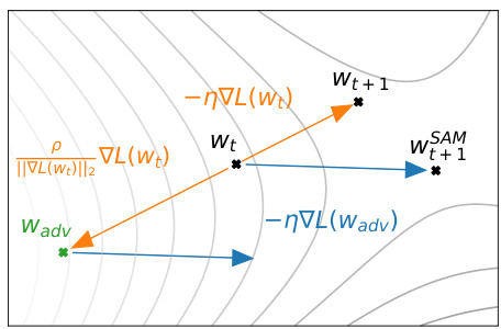
Figure 2: Schematic of the SAM parameter update.
图 2: SAM参数更新示意图。
3 EMPIRICAL EVALUATION
3 实证评估
In order to assess SAM’s efficacy, we apply it to a range of different tasks, including image classification from scratch (including on CIFAR-10, CIFAR-100, and ImageNet), finetuning pretrained models, and learning with noisy labels. In all cases, we measure the benefit of using SAM by simply replacing the optimization procedure used to train existing models with SAM, and computing the resulting effect on model generalization. As seen below, SAM materially improves generalization performance in the vast majority of these cases.
为了评估SAM的有效性,我们将其应用于一系列不同任务,包括从零开始的图像分类(包括CIFAR-10、CIFAR-100和ImageNet)、微调预训练模型以及带噪声标签的学习。在所有情况下,我们通过简单地将现有模型的训练优化过程替换为SAM来衡量其优势,并计算对模型泛化能力的影响。如下所示,SAM在绝大多数情况下显著提升了泛化性能。
3.1 IMAGE CLASSIFICATION FROM SCRATCH
3.1 从零开始的图像分类
We first evaluate SAM’s impact on generalization for today’s state-of-the-art models on CIFAR-10 and CIFAR-100 (without pre training): Wide Res Nets with ShakeShake regular iz ation (Zagoruyko & Komodakis, 2016; Gastaldi, 2017) and PyramidNet with ShakeDrop regular iz ation (Han et al., 2016; Yamada et al., 2018). Note that some of these models have already been heavily tuned in prior work and include carefully chosen regular iz ation schemes to prevent over fitting; therefore, significantly improving their generalization is quite non-trivial. We have ensured that our implementations’ generalization performance in the absence of SAM matches or exceeds that reported in prior work (Cubuk et al., 2018; Lim et al., 2019)
我们首先评估了SAM在CIFAR-10和CIFAR-100数据集(未经预训练)上对当前最先进模型的泛化性能影响:采用ShakeShake正则化(Wide Res Nets)的模型(Zagoruyko & Komodakis, 2016; Gastaldi, 2017)以及采用ShakeDrop正则化的PyramidNet模型(Han et al., 2016; Yamada et al., 2018)。需要说明的是,这些模型中的部分已在先前工作中经过充分调优,并采用了精心设计的正则化方案以防止过拟合,因此要显著提升其泛化性能并非易事。我们已确保在不使用SAM的情况下,我们的实现方案的泛化性能达到或超越了先前工作(Cubuk et al., 2018; Lim et al., 2019)报告的结果。
All results use basic data augmentations (horizontal flip, padding by four pixels, and random crop). We also evaluate in the setting of more advanced data augmentation methods such as cutout regularization (Devries & Taylor, 2017) and Auto Augment (Cubuk et al., 2018), which are utilized by prior work to achieve state-of-the-art results.
所有结果均采用基础数据增强方法(水平翻转、四周填充四个像素及随机裁剪)。我们还评估了更先进的数据增强方法设置,如cutout正则化 (Devries & Taylor, 2017) 和Auto Augment (Cubuk et al., 2018),这些方法被先前研究用于实现最先进成果。
SAM has a single hyper parameter $\rho$ (the neighborhood size), which we tune via a grid search over ${0.01,0.02,0.05,0.{\bar{1}},0.{\bar{2}},0.5}$ using $10%$ of the training set as a validation set3. Please see appendix C.1 for the values of all hyper parameters and additional training details. As each SAM weight update requires two back propagation operations (one to compute $\hat{\pmb{\epsilon}}(\pmb{w})$ and another to compute the final gradient), we allow each non-SAM training run to execute twice as many epochs as each SAM training run, and we report the best score achieved by each non-SAM training run across either the standard epoch count or the doubled epoch count4. We run five independent replicas of each experimental condition for which we report results (each with independent weight initialization and data shuffling), reporting the resulting mean error (or accuracy) on the test set, and the associated $95%$ confidence interval. Our implementations utilize JAX (Bradbury et al., 2018), and we train all models on a single host having 8 NVidia $\mathrm{V}100\mathrm{GPUs}^{5}$ . To compute the SAM update when parallel i zing across multiple accelerators, we divide each data batch evenly among the accelerators, independently compute the SAM gradient on each accelerator, and average the resulting sub-batch SAM gradients to obtain the final SAM update.
SAM 只有一个超参数 $\rho$(邻域大小),我们通过在 ${0.01,0.02,0.05,0.{\bar{1}},0.{\bar{2}},0.5}$ 上进行网格搜索来调整该参数,并使用训练集的 $10%$ 作为验证集。所有超参数的具体取值及其他训练细节请参阅附录 C.1。由于每次 SAM 权重更新需要两次反向传播操作(一次计算 $\hat{\pmb{\epsilon}}(\pmb{w})$,另一次计算最终梯度),我们让非 SAM 训练运行的 epoch 数是 SAM 训练的两倍,并报告非 SAM 训练在标准 epoch 数或双倍 epoch 数下取得的最佳分数。我们对每个实验条件进行了五次独立重复(每次使用独立的权重初始化和数据打乱),报告测试集上的平均误差(或准确率)及相应的 $95%$ 置信区间。我们的实现基于 JAX (Bradbury et al., 2018),所有模型均在配备 8 块 NVidia $\mathrm{V}100\mathrm{GPUs}^{5}$ 的单台主机上训练。在多加速器并行计算 SAM 更新时,我们将每个数据批次均匀分配给各加速器,在各加速器上独立计算 SAM 梯度,最后对子批次的 SAM 梯度取平均以获得最终的 SAM 更新。
As seen in Table 1, SAM improves generalization across all settings evaluated for CIFAR-10 and CIFAR-100. For example, SAM enables a simple WideResNet to attain $1.6%$ test error, versus $2.2%$ error without SAM. Such gains have previously been attainable only by using more complex model architectures (e.g., PyramidNet) and regular iz ation schemes (e.g., Shake-Shake, ShakeDrop); SAM provides an easily-implemented, model-independent alternative. Furthermore, SAM delivers improvements even when applied atop complex architectures that already use sophisticated regularization: for instance, applying SAM to a PyramidNet with ShakeDrop regular iz ation yields $10.3%$ error on CIFAR-100, which is, to our knowledge, a new state-of-the-art on this dataset without the use of additional data.
如表 1 所示,SAM (Sharpness-Aware Minimization) 在所有评估的 CIFAR-10 和 CIFAR-100 设置中都提高了泛化性能。例如,SAM 使简单的 WideResNet 实现了 1.6% 的测试错误率,而未使用 SAM 时为 2.2%。此前,这样的提升只能通过使用更复杂的模型架构(如 PyramidNet)和正则化方案(如 Shake-Shake、ShakeDrop)来实现;而 SAM 提供了一种易于实现、与模型无关的替代方案。此外,即使在已使用复杂正则化的架构上应用 SAM 仍能带来改进:例如,在采用 ShakeDrop 正则化的 PyramidNet 上应用 SAM 后,CIFAR-100 的错误率降至 10.3%,据我们所知,这是不使用额外数据时该数据集上的新最优结果。
Beyond CIFAR ${10,100}$ , we have also evaluated SAM on the SVHN (Netzer et al., 2011) and Fashion-MNIST datasets (Xiao et al., 2017). Once again, SAM enables a simple WideResNet to achieve accuracy at or above the state-of-the-art for these datasets: $0.99%$ error for SVHN, and $3.59%$ for Fashion-MNIST. Details are available in appendix B.1.
除了 CIFAR ${10,100}$ 之外,我们还在 SVHN (Netzer et al., 2011) 和 Fashion-MNIST (Xiao et al., 2017) 数据集上评估了 SAM。结果表明,SAM 能让简单的 WideResNet 在这些数据集上达到或超越当前最优水平:SVHN 错误率为 $0.99%$,Fashion-MNIST 错误率为 $3.59%$。详细结果见附录 B.1。
To assess SAM’s performance at larger scale, we apply it to ResNets (He et al., 2015) of different depths (50, 101, 152) trained on ImageNet (Deng et al., 2009). In this setting, following prior work (He et al., 2015; Szegedy et al., 2015), we resize and crop images to 224-pixel resolution, normalize them, and use batch size 4096, initial learning rate 1.0, cosine learning rate schedule, SGD optimizer with momentum 0.9, label smoothing of 0.1, and weight decay 0.0001. When applying SAM, we use $\rho=0.05$ (determined via a grid search on ResNet-50 trained for 100 epochs). We train all models on ImageNet for up to 400 epochs using a Google Cloud TPUv3 and report top-1 and top-5 test error rates for each experimental condition (mean and $95%$ confidence interval across 5 independent runs).
为了评估SAM在大规模场景下的性能,我们将其应用于不同深度(50、101、152层)的ResNet (He et al., 2015)模型在ImageNet (Deng et al., 2009)数据集上的训练。本实验遵循前人工作(He et al., 2015; Szegedy et al., 2015)的设置:将图像缩放裁剪至224像素分辨率并进行归一化处理,使用批量大小4096、初始学习率1.0、余弦学习率调度、动量0.9的SGD优化器、标签平滑系数0.1以及权重衰减0.0001。应用SAM时,我们设定$\rho=0.05$(该参数通过在ResNet-50上进行100轮训练的网格搜索确定)。所有模型均在Google Cloud TPUv3上训练400轮,每种实验条件下报告top-1和top-5测试错误率(取5次独立运行的平均值及$95%$置信区间)。
| 模型 | 数据增强 | CIFAR-10 SAM | CIFAR-10 SGD | CIFAR-100 SAM | CIFAR-100 SGD |
|---|---|---|---|---|---|
| WRN-28-10 (200 epochs) WRN-28-10 (200 epochs) WRN-28-10 (200 epochs) | Basic Cutout AA | 2.7±0.1 2.3±0.1 2.1±<0.1 | 3.5±0.1 2.6±0.1 2.3±0.1 | 16.5±0.2 14.9±0.2 13.6±0.2 | 18.8±0.2 16.9±0.1 |
| WRN-28-10 (1800 epochs) WRN-28-10 (1800 epochs) WRN-28-10 (1800 epochs) | Basic Cutout AA | 2.4±0.1 2.1±0.1 1.6±0.1 | 3.5±0.1 2.7±0.1 2.2±<0.1 | 16.3±0.2 14.0±0.1 12.8±0.2 | 15.8±0.2 19.1±0.1 17.4±0.1 16.1±0.2 |
| Shake-Shake (26 2x96d) Shake-Shake (26 2x96d) Shake-Shake (26 2x96d) | Basic Cutout AA | 2.3±<0.1 2.0±<0.1 1.6±<0.1 | 2.7±0.1 2.3±0.1 1.9±0.1 | 15.1±0.1 14.2±0.2 12.8±0.1 | 17.0±0.1 15.7±0.2 |
| PyramidNet PyramidNet PyramidNet | Basic Cutout AA | 2.7±0.1 1.9±0.1 1.6±0.1 | 4.0±0.1 2.5±0.1 1.9±0.1 | 14.6±0.4 12.6±0.2 | 14.1±0.2 19.7±0.3 16.4±0.1 |
| PyramidNet+ShakeDrop PyramidNet+ShakeDrop PyramidNet+ShakeDrop | Basic Cutout AA | 2.1±0.1 1.6±<0.1 1.4±<0.1 | 2.5±0.1 1.9±0.1 1.6±<0.1 | 11.6±0.1 13.3±0.2 11.3±0.1 10.3±0.1 | 14.6±0.1 14.5±0.1 11.8±0.2 10.6±0.1 |
As seen in Table 2, SAM again consistently improves performance, for example improving the ImageNet top-1 error rate of ResNet-152 from $20.3%$ to $18.4%$ . Furthermore, note that SAM enables increasing the number of training epochs while continuing to improve accuracy without over fitting. In contrast, the standard training procedure (without SAM) generally significantly overfits as training extends from 200 to 400 epochs.
如表 2 所示,SAM 再次持续提升性能,例如将 ResNet-152 在 ImageNet 上的 top-1 错误率从 $20.3%$ 降至 $18.4%$。此外需注意,SAM 能够通过增加训练周期数持续提升准确率而不会过拟合。相比之下,标准训练流程(未使用 SAM)在训练周期从 200 增至 400 时通常会出现显著过拟合。
Table 2: Test error rates for ResNets trained on ImageNet, with and without SAM.
表 2: 在ImageNet上训练的ResNet模型使用SAM与不使用SAM时的测试错误率
| 模型 | 训练轮数 | SAM-Top-1 | SAM-Top-5 | 标准训练(NoSAM)-Top-1 | 标准训练(NoSAM)-Top-5 |
|---|---|---|---|---|---|
| ResNet-50 | 100 | 22.5±0.1 | 6.28±0.08 | 22.9±0.1 | 6.62±0.11 |
| 200 | 21.4±0.1 | 5.82±0.03 | 22.3±0.1 | 6.37±0.04 | |
| 400 | 20.9±0.1 | 5.51±0.03 | 22.3±0.1 | 6.40±0.06 | |
| ResNet-101 | 100 | 20.2±0.1 | 5.12±0.03 | 21.2±0.1 | 5.66±0.05 |
| 200 | 19.4±0.1 | 4.76±0.03 | 20.9±0.1 | 5.66±0.04 | |
| 400 | 19.0±<0.01 | 4.65±0.05 | 22.3±0.1 | 6.41±0.06 | |
| ResNet-152 | 100 | 19.2±<0.01 | 4.69±0.04 | 20.4±<0.0 | 5.39±0.06 |
| 200 | 18.5±0.1 | 4.37±0.03 | 20.3±0.2 | 5.39±0.07 | |
| 400 | 18.4±<0.01 | 4.35±0.04 | 20.9±<0.0 | 5.84±0.07 |
3.2 FINETUNING
3.2 微调 (Finetuning)
Transfer learning by pre training a model on a large related dataset and then finetuning on a smaller target dataset of interest has emerged as a powerful and widely used technique for producing highquality models for a variety of different tasks. We show here that SAM once again offers considerable benefits in this setting, even when finetuning extremely large, state-of-the-art, already high-performing models.
通过在大规模相关数据集上预训练模型,再针对特定小规模目标数据集进行微调 (finetuning) 的迁移学习 (transfer learning) 方法,已成为生成各类高质量模型的强大且广泛应用的技术。本文表明,即使在对性能已达顶尖水平的超大规模模型进行微调时,SAM 仍能在此场景下展现出显著优势。
In particular, we apply SAM to finetuning Eff i cent Net-b7 (pretrained on ImageNet) and Efficient Net-L2 (pretrained on ImageNet plus unlabeled JFT; input resolution 475) (Tan & Le, 2019; Kornblith et al., 2018; Huang et al., 2018). We initialize these models to publicly available checkpoints6 trained with Rand Augment $84.7%$ accuracy on ImageNet) and Noisy Student $88.2%$ accuracy on ImageNet), respectively. We finetune these models on each of several target datasets by training each model starting from the aforementioned checkpoint; please see the appendix for details of the hyper parameters used. We report the mean and $95%$ confidence interval of top-1 test error over 5 independent runs for each dataset.
具体而言,我们应用SAM对EfficientNet-b7(基于ImageNet预训练)和EfficientNet-L2(基于ImageNet及未标注JFT数据预训练,输入分辨率475)进行微调 (Tan & Le, 2019; Kornblith et al., 2018; Huang et al., 2018)。这些模型初始化为公开可用的检查点6,分别采用Rand Augment(ImageNet准确率84.7%)和Noisy Student(ImageNet准确率88.2%)训练所得。我们从上述检查点开始,针对每个目标数据集微调模型,具体超参数设置详见附录。对于每个数据集,我们报告5次独立运行的top-1测试错误率均值及95%置信区间。
As seen in Table 3, SAM uniformly improves performance relative to finetuning without SAM. Furthermore, in many cases, SAM yields novel state-of-the-art performance, including $0.30%$ error on CIFAR-10, $3.92%$ error on CIFAR-100, and $11.39%$ error on ImageNet.
如表 3 所示,相对于不使用 SAM (Sharpness-Aware Minimization) 的微调方法,SAM 一致性地提升了性能。此外,在许多情况下,SAM 实现了新的最先进性能,包括 CIFAR-10 上 0.30% 的错误率、CIFAR-100 上 3.92% 的错误率以及 ImageNet 上 11.39% 的错误率。
Table 3: Top-1 error rates for finetuning Efficient Net-b7 (left; ImageNet pre training only) and Efficient Net-L2 (right; pre training on ImageNet plus additional data, such as JFT) on various downstream tasks. Previous state-of-the-art (SOTA) includes Efficient Net (EffNet) (Tan & Le, 2019), Gpipe (Huang et al., 2018), DAT (Ngiam et al., 2018), BiT-M/L (Kolesnikov et al., 2020), KD- forAA (Wei et al., 2020), TBMSL-Net (Zhang et al., 2020), and ViT (Do sov it ski y et al., 2020).
表 3: 在不同下游任务上微调 Efficient Net-b7 (左;仅使用 ImageNet 预训练) 和 Efficient Net-L2 (右;使用 ImageNet 及额外数据如 JFT 预训练) 的 Top-1 错误率。先前的最先进技术 (SOTA) 包括 Efficient Net (EffNet) (Tan & Le, 2019)、Gpipe (Huang et al., 2018)、DAT (Ngiam et al., 2018)、BiT-M/L (Kolesnikov et al., 2020)、KD- forAA (Wei et al., 2020)、TBMSL-Net (Zhang et al., 2020) 和 ViT (Do sov it ski y et al., 2020)。
| 数据集 | EffNet-b7 + SAM | EffNet-b7 | Prev.SOTA (仅ImageNet) | EffNet-L2 + SAM | EffNet-L2 | Prev.SOTA |
|---|---|---|---|---|---|---|
| FGVC_Aircraft | 6.80±0.06 | 8.15±0.08 | 5.3(TBMSL-Net) | 4.82±0.08 | 5.80±0.1 | 5.3(TBMSL-Net) |
| Flowers | 0.63±0.02 | 1.16±0.05 | 0.7 (BiT-M) | 0.35±0.01 | 0.40±0.02 | 0.37(EffNet) |
| Oxford_IT_Pets | 3.97±0.04 | 4.24±0.09 | 4.1 (Gpipe) | 2.90±0.04 | 3.08±0.04 | 4.1 (Gpipe) |
| Stanford_Cars | 5.18±0.02 | 5.94±0.06 | 5.0(TBMSL-Net) | 4.04±0.03 | 4.93±0.04 | 3.8 (DAT) |
| CIFAR-10 | 0.88±0.02 | 0.95±0.03 | 1 (Gpipe) | 0.30±0.01 | 0.34±0.02 | 0.63 (BiT-L) |
| CIFAR-100 | 7.44±0.06 | 7.68±0.06 | 7.83 (BiT-M) | 3.92±0.06 | 4.07±0.08 | 6.49 (BiT-L) |
| Birdsnap | 13.64±0.15 | 14.30±0.18 | 15.7 (EffNet) | 9.93±0.15 | 10.31±0.15 | 14.5 (DAT) |
| Food101 | 7.02±0.02 | 7.17±0.03 | 7.0 (Gpipe) | 3.82±0.01 | 3.97±0.03 | 4.7 (DAT) |
| ImageNet | 15.14±0.03 | 15.3 | 14.2(KDforAA) | 11.39±0.02 | 11.8 | 11.45 (ViT) |
The fact that SAM seeks out model parameters that are robust to perturbations suggests SAM’s potential to provide robustness to noise in the training set (which would perturb the training loss landscape). Thus, we assess here the degree of robustness that SAM provides to label noise.
SAM寻找对扰动具有鲁棒性的模型参数这一事实表明,它可能增强训练集噪声(会扰动训练损失曲面)的鲁棒性。因此,我们在此评估SAM对标签噪声的鲁棒性程度。
In particular, we measure the effect of applying SAM in the classical noisy-label setting for CIFAR-10, in which a fraction of the training set’s labels are randomly flipped; the test set remains unmodified (i.e., clean). To ensure valid comparison to prior work, which often utilizes architectures specialized to the noisy-label setting, we train a simple model of similar size (ResNet-32) for 200 epochs, following Jiang et al. (2019). We evaluate five variants of model training: standard SGD, SGD with Mixup (Zhang et al., 2017), SAM, and ”boots trapped” variants of SGD with Mixup and SAM (wherein the model is first trained as usual and then retrained from scratch on the labels predicted by the initially trained model). When applying SAM, we use $\rho=0.1$ for all noise levels except $80%$ , for which we use $\rho=0.05$ for more stable convergence. For the Mixup baselines, we tried all values of $\alpha\in{1,8,16,32}$ and conservatively report the best score for each noise level.
具体而言,我们在CIFAR-10的经典噪声标签设置中测量了应用SAM(Sharpness-Aware Minimization)的效果,该设置会随机翻转训练集中一定比例的标签,而测试集保持不变(即干净数据)。为确保与先前工作的有效对比(这些工作通常采用专为噪声标签场景设计的架构),我们按照Jiang等人(2019)的方法,训练了一个规模相近的简单模型(ResNet-32)200个周期。我们评估了五种模型训练变体:标准SGD、带Mixup的SGD(Zhang等人,2017)、SAM,以及带Mixup和SAM的"自举"变体(即先常规训练模型,然后根据初始训练模型预测的标签从头开始重新训练)。应用SAM时,除80%噪声水平使用$\rho=0.05$以获得更稳定的收敛外,其余噪声水平均采用$\rho=0.1$。对于Mixup基线,我们测试了$\alpha\in{1,8,16,32}$的所有取值,并保守地报告每个噪声水平下的最佳得分。
Table 4: Test accuracy on the clean test set for models trained on CIFAR-10 with noisy labels. Lower block is our implementation, upper block gives scores from the literature, per Jiang et al. (2019).
表 4: 在带噪声标签的CIFAR-10数据集上训练模型在干净测试集上的准确率。下方区块为我们的实现结果,上方区块为Jiang等人(2019)文献中的得分。
| 方法 | 20 | 40 | 60 | 80 |
|---|---|---|---|---|
| Sanchez等人(2019) | 94.0 | 92.8 | 90.3 | 74.1 |
| Zhang&Sabuncu (2018) | 89.7 | 87.6 | 82.7 | 67.9 |
| Lee等人(2019) | 87.1 | 81.8 | 75.4 | |
| Chen等人(2019) | 89.7 | 52.3 | ||
| Huang等人(2019) | 92.6 | 90.3 | 43.4 | |
| MentorNet(2017) | 92.0 | 91.2 | 74.2 | 60.0 |
| Mixup (2017) | 94.0 | 91.5 | 86.8 | 76.9 |
| MentorMix(2019) | 95.6 | 94.2 | 91.3 | 81.0 |
| SGD | 84.8 | 68.8 | 48.2 | 26.2 |
| Mixup | 93.0 | 90.0 | 83.8 | 70.2 |
| Bootstrap+Mixup | 93.3 | 92.0 | 87.6 | 72.0 |
| SAM | 95.1 | 93.4 | 90.5 | 77.9 |
| Bootstrap+SAM | 95.4 | 94.2 | 91.8 | 79.9 |
As seen in Table 4, SAM provides a high degree of robustness to label noise, on par with that provided by state-of-the art procedures that specifically target learning with noisy labels. Indeed, simply training a model with SAM outperforms all prior methods specifically targeting label noise robustness, with the exception of MentorMix (Jiang et al., 2019). However, simply boots trapping SAM yields performance comparable to that of MentorMix (which is substantially more complex).
如表 4 所示,SAM (Sharpness-Aware Minimization) 对标签噪声具有高度鲁棒性,其表现与专门针对含噪声标签学习的最先进方法相当。事实上,仅使用 SAM 训练模型就超越了所有专门针对标签噪声鲁棒性的先前方法,除了 MentorMix (Jiang et al., 2019)。然而,简单地通过自助采样 (bootstrap) 增强 SAM 即可获得与 MentorMix 相当的性能 (后者实现复杂度显著更高)。

Figure 3: (left) Evolution of the spectrum of the Hessian during training of a model with standard SGD (lefthand column) or SAM (righthand column). (middle) Test error as a function of $\rho$ for different values of $m$ . (right) Predictive power of $m$ -sharpness for the generalization gap, for different values of $m$ (higher means the sharpness measure is more correlated with actual generalization gap).
图 3: (左) 使用标准 SGD (左列) 或 SAM (右列) 训练模型时 Hessian 矩阵谱的演变。(中) 测试误差随 $\rho$ 变化的函数关系,针对不同的 $m$ 值。(右) 不同 $m$ 值下 $m$-锐度对泛化间隙的预测能力 (数值越高表示锐度度量与实际泛化间隙相关性越强)。
4 SHARPNESS AND GENERALIZATION THROUGH THE LENS OF SAM
4 通过SAM视角看锐度与泛化性
4.1 $m$ -SHARPNESS
4.1 $m$-SHARPNESS
Though our derivation of SAM defines the SAM objective over the entire training set, when utilizing SAM in practice, we compute the SAM update per-batch (as described in Algorithm 1) or even by averaging SAM updates computed independently per-accelerator (where each accelerator receives a subset of size $m$ of a batch, as described in Section 3). This latter setting is equivalent to modifying the SAM objective (equation 1) to sum over a set of independent $\epsilon$ maximization s, each performed on a sum of per-data-point losses on a disjoint subset of $m$ data points, rather than performing the $\epsilon$ maximization over a global sum over the training set (which would be equivalent to setting $m$ to the total training set size). We term the associated measure of sharpness of the loss landscape $m$ -sharpness.
虽然我们对SAM(Sharpness-Aware Minimization)的推导是在整个训练集上定义其目标函数,但在实际应用中,我们采用逐批次计算SAM更新(如算法1所述)的方式,甚至通过平均各加速器独立计算的SAM更新来实现(每个加速器处理批次中大小为$m$的子集,详见第3节)。后一种设置相当于修改SAM目标函数(公式1),使其对一组独立的$\epsilon$最大化过程求和——每个过程针对$m$个数据点的不相交子集上的逐点损失之和进行,而非在训练集的全局求和上执行$\epsilon$最大化(这将等价于设置$m$为训练集总大小)。我们将这种损失景观的锐度度量称为$m$-锐度。
To better understand the effect of $m$ on SAM, we train a small ResNet on CIFAR-10 using SAM with a range of values of $m$ . As seen in Figure 3 (middle), smaller values of $m$ tend to yield models having better generalization ability. This relationship fortuitously aligns with the need to parallel ize across multiple accelerators in order to scale training for many of today’s models.
为了更好地理解 $m$ 对 SAM (Sharpness-Aware Minimization) 的影响,我们在 CIFAR-10 数据集上使用不同 $m$ 值训练了一个小型 ResNet。如图 3 (中) 所示,较小的 $m$ 值往往能产生具有更好泛化能力的模型。这种关系恰好与当今许多模型训练规模化所需的跨多加速器并行需求相吻合。
Intriguingly, the $m$ -sharpness measure described above furthermore exhibits better correlation with models’ actual generalization gaps as $m$ decreases, as demonstrated by Figure 3 (right)7. In particular, this implies that $m$ -sharpness with $m<n$ yields a better predictor of generalization than the full-training-set measure suggested by Theorem 1 in Section 2 above, suggesting an interesting new avenue of future work for understanding generalization.
有趣的是,如图3 (右) 所示,随着 $m$ 减小,上述 $m$-sharpness指标与模型实际泛化差距的相关性会进一步增强。特别地,这意味着当 $m<n$ 时,$m$-sharpness比第2节定理1建议的完整训练集指标更能预测泛化性能,这为理解泛化问题开辟了一条值得探索的新研究方向。
4.2 HESSIAN SPECTRA
4.2 海森矩阵谱
Motivated by the connection between geometry of the loss landscape and generalization, we constructed SAM to seek out minima of the training loss landscape having both low loss value and low curvature (i.e., low sharpness). To further confirm that SAM does in fact find minima having low curvature, we compute the spectrum of the Hessian for a Wide Res Net 40-10 trained on CIFAR-10 for 300 steps both with and without SAM (without batch norm, which tends to obscure interpretation of the Hessian), at different epochs during training. Due to the parameter space’s dimensionality, we approximate the Hessian spectrum using the Lanczos algorithm of Ghorbani et al. (2019).
受损失函数几何特性与泛化能力之间关联的启发,我们构建了SAM(Sharpness-Aware Minimization)方法,旨在寻找兼具低损失值和低曲率(即低锐度)的训练损失函数极小值点。为验证SAM确实能发现低曲率极小值,我们分别在训练过程中不同阶段,对使用/未使用SAM(移除了批归一化层以避免干扰Hessian矩阵解释性)的Wide ResNet 40-10模型(CIFAR-10数据集训练300步)计算Hessian矩阵谱。鉴于参数空间的高维度特性,我们采用Ghorbani等人 (2019) 提出的Lanczos算法对Hessian谱进行近似计算。
Figure 3 (left) reports the resulting Hessian spectra. As expected, the models trained with SAM converge to minima having lower curvature, as seen in the overall distribution of eigenvalues, the maximum eigenvalue $(\lambda_{\mathrm{max}})$ at convergence (approximately 24 without SAM, 1.0 with SAM), and the bulk of the spectrum (the ratio $\lambda_{\mathrm{{max}}}/\lambda_{5}$ , commonly used as a proxy for sharpness (J as tr zeb ski et al., 2020); up to 11.4 without SAM, and 2.6 with SAM).
图 3 (左) 展示了所得Hessian谱。正如预期,使用SAM (Sharpness-Aware Minimization) 训练的模型收敛至曲率更低的极小值点,这体现在:特征值的整体分布、收敛时的最大特征值 $(\lambda_{\mathrm{max}})$ (无SAM时约24,使用SAM时为1.0) 以及谱的主体部分 (常用作尖锐度指标的比值 $\lambda_{\mathrm{max}}/\lambda_{5}$ (Jastrzebski et al., 2020);无SAM时高达11.4,使用SAM时为2.6)。
5 RELATED WORK
5 相关工作
The idea of searching for “flat” minima can be traced back to Hochreiter & Schmid huber (1995), and its connection to generalization has seen significant study (Shirish Keskar et al., 2016; Dziugaite & Roy, 2017; Neyshabur et al., 2017; Dinh et al., 2017). In a recent large scale empirical study, Jiang et al. (2019) studied 40 complexity measures and showed that a sharpness-based measure has highest correlation with generalization, which motivates penalizing sharpness. Hochreiter & Schmid huber (1997) was perhaps the first paper on penalizing the sharpness, regularizing a notion related to Minimum Description Length (MDL). Other ideas which also penalize sharp minima include operating on diffused loss landscape (Mobahi, 2016) and regularizing local entropy (Chaudhari et al., 2016). Another direction is to not penalize the sharpness explicitly, but rather average weights during training; Izmailov et al. (2018) showed that doing so can yield flatter minima that can also generalize better. However, the measures of sharpness proposed previously are difficult to compute and differentiate through. In contrast, SAM is highly scalable as it only needs two gradient computations per iteration. The concurrent work of Sun et al. (2020) focuses on resilience to random and adversarial corruption to expose a model’s vulnerabilities; this work is perhaps closest to ours. Our work has a different basis: we develop SAM motivated by a principled starting point in generalization, clearly demonstrate SAM’s efficacy via rigorous large-scale empirical evaluation, and surface important practical and theoretical facets of the procedure (e.g., $m$ -sharpness). The notion of all-layer margin introduced by Wei & Ma (2020) is closely related to this work; one is adversarial perturbation over the activation s of a network and the other over its weights, and there is some coupling between these two quantities.
寻找"平坦"最小值的思路可追溯至Hochreiter & Schmidhuber (1995),其与泛化性的关联已得到广泛研究 (Shirish Keskar等, 2016; Dziugaite & Roy, 2017; Neyshabur等, 2017; Dinh等, 2017)。Jiang等 (2019) 在近期大规模实证研究中分析了40种复杂度度量,发现基于锐度的指标与泛化性相关性最高,这启发了对锐度进行惩罚的思路。Hochreiter & Schmidhuber (1997) 可能是首篇研究锐度惩罚的论文,通过正则化与最小描述长度 (MDL) 相关的概念来实现。其他惩罚尖锐最小值的方法包括在扩散损失曲面上操作 (Mobahi, 2016) 和正则化局部熵 (Chaudhari等, 2016)。另一类方法不显式惩罚锐度,而是在训练过程中对权重进行平均:Izmailov等 (2018) 证明该方法能获得更平坦且泛化性更好的最小值。但既有锐度度量方法存在计算和微分困难,而SAM仅需每次迭代两次梯度计算,具有高度可扩展性。Sun等 (2020) 的同期工作聚焦模型对随机和对抗破坏的鲁棒性以暴露脆弱性,与本研究最为接近。我们的工作基于不同出发点:从泛化性的理论基点推导SAM,通过严谨的大规模实证评估验证其效能,并揭示了该方法的重要实践与理论特性 (如$m$-锐度)。Wei & Ma (2020) 提出的全层间隔概念与本工作紧密相关:前者针对网络激活的对抗扰动,后者针对权重扰动,二者存在一定耦合关系。
6 DISCUSSION AND FUTURE WORK
6 讨论与未来工作
In this work, we have introduced SAM, a novel algorithm that improves generalization by simultaneously minimizing loss value and loss sharpness; we have demonstrated SAM’s efficacy through a rigorous large-scale empirical evaluation. We have surfaced a number of interesting avenues for future work. On the theoretical side, the notion of per-data-point sharpness yielded by $m$ -sharpness (in contrast to global sharpness computed over the entire training set, as has typically been studied in the past) suggests an interesting new lens through which to study generalization. Methodological ly, our results suggest that SAM could potentially be used in place of Mixup in robust or semi-supervised methods that currently rely on Mixup (giving, for instance, MentorSAM). We leave to future work a more in-depth investigation of these possibilities.
在本工作中,我们提出了SAM(一种通过同时最小化损失值和损失锐度来提升泛化能力的新算法),并通过严格的大规模实证评估验证了其有效性。我们为未来研究揭示了若干有趣的方向:在理论层面,由$m$-锐度(与过去通常研究的基于整个训练集计算的全局锐度相对)得出的逐数据点锐度概念,为研究泛化性提供了新颖视角;在方法论层面,我们的结果表明SAM或可替代当前依赖Mixup的鲁棒/半监督方法中的Mixup(例如衍生出MentorSAM)。这些可能性的深入探索将留待未来工作。