SA-DVAE: Improving Zero-Shot Skeleton-Based Action Recognition by Disentangled Variation al Auto encoders
SA-DVAE: 通过解耦变分自编码器改进零样本骨骼动作识别
Abstract. Existing zero-shot skeleton-based action recognition methods utilize projection networks to learn a shared latent space of skeleton features and semantic embeddings. The inherent imbalance in action recognition datasets, characterized by variable skeleton sequences yet constant class labels, presents significant challenges for alignment. To address the imbalance, we propose SA-DVAE—Semantic Alignment via Disentangled Variation al Auto encoders, a method that first adopts feature disentanglement to separate skeleton features into two independent parts—one is semantic-related and another is irrelevant—to better align skeleton and semantic features. We implement this idea via a pair of modality-specific variation al auto encoders coupled with a total correction penalty. We conduct experiments on three benchmark datasets: NTU RGB+D, NTU RGB+D 120 and PKU-MMD, and our experimental results show that SA-DAVE produces improved performance over existing methods. The code is available at https://github.com/ pha123661/SA-DVAE.
摘要。现有基于骨架的零样本动作识别方法利用投影网络学习骨架特征与语义嵌入的共享潜在空间。动作识别数据集固有的不平衡性(表现为多变的骨架序列与固定的类别标签)给特征对齐带来了巨大挑战。为解决这一问题,我们提出SA-DVAE——基于解耦变分自编码器的语义对齐方法,该方法通过特征解耦将骨架特征分离为语义相关与无关两个独立部分,以实现更好的骨架-语义特征对齐。我们通过一对模态特定的变分自编码器配合总体校正惩罚项实现该构想。在NTU RGB+D、NTU RGB+D 120和PKU-MMD三个基准数据集上的实验表明,SA-DVAE相较现有方法取得了性能提升。代码已开源:https://github.com/pha123661/SA-DVAE。
Keywords: Skeleton-based Action Recognition $\cdot$ Zero-Shot and Generalized Zero-Shot Learning · Feature Disentanglement
关键词: 基于骨架的动作识别 $\cdot$ 零样本与广义零样本学习 · 特征解耦
1 Introduction
1 引言
Action recognition is a long-standing active research area because it is challenging and has a wide range of applications like surveillance, monitoring, and human-computer interfaces. Based on input data types, there are several lines of studies on human action recognition: image-based, video-based, depth-based, and skeleton-based. In this paper, we focus on the skeleton-based action recognition, which is enabled by the advance in pose estimation [24,27] and sensor [14,28] technologies, and has emerged as a viable alternative to video-based action recognition due to its resilience to variations in appearance and background. Some existing skeleton-based action recognition methods already achieve remarkable performance on large-scale action recognition datasets [5, 17, 23] through supervised learning, but labeling data is expensive and time-consuming. For the cases where training data are difficult to obtain or prevented by privacy issues, zeroshot learning (ZSL) offers an alternative solution by recognizing unseen actions through supporting information such as the names, attributes, or descriptions of the unseen classes. Therefore, zero-shot learning has multiple types of input data and aims to learn an effective way of dealing with those data representations. For skeleton-based zero-shot action recognition, several methods have been proposed to align skeleton features and text features in the same space.
动作识别是一个长期活跃的研究领域,因其具有挑战性且应用广泛,如监控、监测和人机交互等。根据输入数据类型,人体动作识别研究可分为基于图像、视频、深度和骨骼的几类方法。本文聚焦于基于骨骼的动作识别,该技术得益于姿态估计[24,27]和传感器[14,28]技术的进步,因其对外观和背景变化的鲁棒性,已成为视频动作识别的可行替代方案。现有部分基于骨骼的动作识别方法通过监督学习已在大规模动作识别数据集[5,17,23]上取得显著性能,但数据标注成本高昂且耗时。对于训练数据难以获取或受隐私问题限制的场景,零样本学习(ZSL)通过利用未见类别的名称、属性或描述等辅助信息来识别未知动作,提供了替代解决方案。因此,零样本学习涉及多种输入数据类型,旨在学习处理这些数据表征的有效方法。针对基于骨骼的零样本动作识别,已有多种方法提出将骨骼特征与文本特征对齐到同一空间。
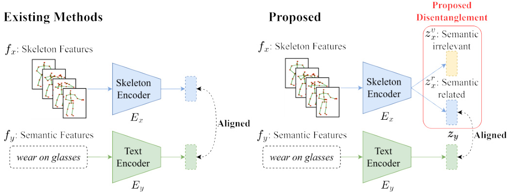
Fig. 1: Comparison with existing methods. Our method is the first to apply feature disentanglement to the problem of skeleton-based zero-shot action recognition. All existing methods directly align skeleton features with textual ones, but ours only aligns a part of semantic-related skeleton features with the textual ones.
图 1: 与现有方法的对比。我们的方法是首个将特征解耦 (feature disentanglement) 应用于基于骨架的零样本动作识别问题的方法。现有方法都直接将骨架特征与文本特征对齐,而我们仅将语义相关的部分骨架特征与文本特征对齐。
However, to the best of our knowledge, all existing methods assume that the group of skeleton sequences are well captured and highly consistent so their ideas mainly focus on how to semantically optimize text representation. After carefully examining the source videos in two widely used benchmark datasets NTU RGB+D and PKU-MMD, we found the assumption is questionable. We observe that for some labels, the camera positions and actors’ action differences do bring in significant noise. To address this observation, we seek an effective way to deal with the problem. Inspired by an existing ZSL method [3] which shows semantic-irrelevant features can be separated from semantic-related ones, we propose SA-DVAE for skeleton-based action recognition. SA-DVAE tackles the generalization problem by disentangling the skeleton latent feature space into two components: a semantic-related term and a semantic-irrelevant term as shown in Fig. 1. This enables the model to learn more robust and generalizable visual embeddings by focusing solely on the semantic-related term for action recognition. In addition, SA-DVAE implements a learned total correlation penalty that encourages independence between the two factorized latent features and minimizes the shared information captured by the two representations. This penalty is realized by an adversarial disc rim in at or that aims to estimate the lower bound of the total correlation between the factorized latent features.
然而,据我们所知,现有方法均假设骨架序列组已被完整捕捉且高度一致,因此其核心思路集中于如何从语义层面优化文本表示。通过细致分析NTU RGB+D和PKU-MMD这两个广泛使用的基准数据集中的源视频,我们发现该假设存在疑问。我们观察到,对于某些动作标签,摄像机位姿与演员动作差异确实会引入显著噪声。针对这一现象,我们探索了有效的解决方案。受现有零样本学习方法[3](证明语义无关特征可与语义相关特征分离)的启发,我们提出了基于骨架的动作识别模型SA-DVAE。如图1所示,SA-DVAE通过将骨架潜在特征空间解耦为两个组件来解决泛化问题:语义相关项与语义无关项。该设计使模型能仅聚焦语义相关项进行动作识别,从而学习更具鲁棒性和泛化能力的视觉嵌入。此外,SA-DVAE采用学习型总相关性惩罚机制,通过对抗判别器估算解耦潜在特征间总相关性下界,强制两项特征保持独立性并最小化表征间的共享信息。
The contributions of our paper are as follows:
本文的贡献如下:
2 Related Work
2 相关工作
The proposed SA-DAVE method covers two research fields: zero-shot learning and action recognition, and it uses feature disentanglement to deal with skeleton data noise. Here we discuss the most related research reports in the literature.
提出的SA-DAVE方法涵盖了两个研究领域:零样本学习和动作识别,并利用特征解耦处理骨骼数据噪声。以下我们讨论文献中最相关的研究报告。
Skeleton-Based Zero-Shot Action Recognition. ZSL aims to train a model under the condition that some classes are unseen during training. The more challenging GZSL expands the task to classify both seen and unseen classes during testing [19]. ZSL relies on semantic information to bridge the gap between seen and unseen classes.
基于骨架的零样本动作识别。ZSL旨在训练一个模型,使其在训练过程中某些类别不可见的情况下仍能工作。更具挑战性的GZSL将任务扩展为在测试时同时分类可见和不可见类别[19]。ZSL依赖语义信息来弥合可见与不可见类别之间的鸿沟。
Existing methods address the skeleton and text zero-shot action recognition problem by constructing a shared space for both modalities. ReViSE [13] learns auto encoders for each modality and aligns them by minimizing the maximum mean discrepancy loss between the latent spaces. Building on the concept of feature generation, CADA-VAE [22] employs variation al auto encoders (VAEs) for each modality, aligning the latent spaces through cross-modal reconstruction and minimizing the Wasser stein distance between the inference models. These methods then learn class if i ers on the shared space to conduct classification.
现有方法通过构建两种模态的共享空间来解决骨架和文本零样本动作识别问题。ReViSE [13] 为每种模态学习自动编码器,并通过最小化潜在空间之间的最大均值差异损失来对齐它们。基于特征生成的概念,CADA-VAE [22] 为每种模态使用变分自动编码器 (VAE),通过跨模态重构对齐潜在空间,并最小化推理模型之间的Wasserstein距离。这些方法随后在共享空间上学习分类器以进行分类。
SynSE [8] and JPoSE [25] are two methods that leverage part-of-speech (PoS) information to improve the alignment between text descriptions and their corresponding visual representations. SynSE extends CADA-VAE by decomposing text descriptions by PoS tags, creating individual VAEs for each PoS label, and aligning them in the skeleton space. Similarly, JPoSE [25] learns multiple shared latent spaces for each PoS label using projection networks. JPoSE employs uni-modal triplet loss to maintain the neighborhood structure of each modality within the shared space and cross-modal triplet loss to align the two modalities.
SynSE [8] 和 JPoSE [25] 是两种利用词性 (PoS) 信息来改善文本描述与其对应视觉表征对齐的方法。SynSE 通过按词性标签分解文本描述,为每个词性标签创建独立的 VAE (Variational Autoencoder) ,并在骨架空间中对齐它们,从而扩展了 CADA-VAE。类似地,JPoSE [25] 使用投影网络为每个词性标签学习多个共享潜在空间。JPoSE 采用单模态三元组损失来保持共享空间内各模态的邻域结构,并采用跨模态三元组损失来对齐两种模态。
On the other hand, SMIE [29] focuses on maximizing mutual information between skeleton and text feature spaces, utilizing a Jensen-Shannon Divergence estimator trained with contrastive learning. It also considers temporal information in action sequences by promoting an increase in mutual information as more frames are observed.
另一方面,SMIE [29] 专注于最大化骨架与文本特征空间之间的互信息,利用通过对比学习训练的 Jensen-Shannon 散度估计器。它还通过促进观察到更多帧时互信息的增加来考虑动作序列中的时序信息。
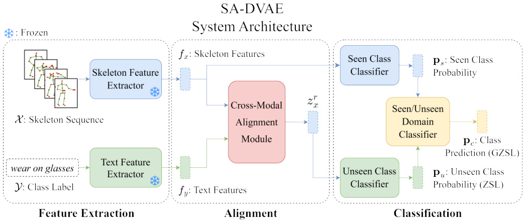
Fig. 2: System Architecture of SA-DVAE. Initially, the feature extractors are employed to extract features. Subsequently, the cross-modal alignment module aligns the two modalities and generates semantic-related unseen skeleton features $(z_{x}^{r}$ ). These generated features are utilized to train class if i ers.
图 2: SA-DVAE系统架构。首先通过特征提取器提取特征,随后跨模态对齐模块对两种模态进行对齐并生成语义相关的未见骨骼特征$(z_{x}^{r}$)。这些生成的特征用于训练分类器。
While JPoSE and SynSE demonstrate the benefits of incorporating PoS information, they rely heavily on it and require additional PoS tagging effort. Furthermore, the two methods neglect the inherent asymmetry between modalities, aligning semantic-related and irrelevant terms to the semantic features and missing the chance to improve recognition accuracy further. In contrast, our approach uses simple class labels without the need of PoS tags, and uses only semantic-related skeleton information to align text data.
虽然JPoSE和SynSE展示了融入词性(PoS)信息的优势,但它们过度依赖该信息且需要额外的词性标注工作。此外,这两种方法忽视了模态间固有的不对称性,将语义相关与无关的术语都对齐到语义特征上,错失了进一步提升识别准确率的机会。相比之下,我们的方法仅使用简单的类别标签而无需词性标注,并且仅利用语义相关的骨架信息来对齐文本数据。
Feature Disentanglement in Generalized Zero-Shot Learning. Feature disentanglement refers to the process of separating the underlying factors of variation in data [2]. Because methods of zero-shot learning are sensitive to the quality of both visual and semantic features, feature disentanglement serves as an effective approach to scrutinize either visual or semantic features, as well as addressing the domain shift problem [19], thereby generating more robust and generalized representations.
广义零样本学习中的特征解耦。特征解耦 (feature disentanglement) 指分离数据中潜在变化因素的过程 [2]。由于零样本学习方法对视觉和语义特征的质量均较为敏感,特征解耦可作为审视视觉/语义特征的有效途径,同时解决域偏移问题 (domain shift) [19],从而生成更具鲁棒性和泛化能力的表征。
SDGZSL [3] decomposes visual embeddings into semantic-consistent and semantic-unrelated components using shared class-level attributes, and learns an additional relation network to maximize compatibility between semanticconsistent representations and their corresponding semantic embeddings. This approach is motivated by the transfer of knowledge from intermediate semantics (e.g., class attributes) to unseen classes. In contrast, SA-DVAE addresses the inherent asymmetry between the text and skeleton modalities, enabling the direct use of text descriptions instead of relying on predefined class attributes.
SDGZSL [3] 利用共享的类级别属性将视觉嵌入分解为语义一致和语义无关的组件,并学习一个额外的关系网络来最大化语义一致表示与其对应语义嵌入之间的兼容性。该方法的动机是将知识从中间语义(如类属性)迁移到未见类别。相比之下,SA-DVAE解决了文本与骨骼模态之间固有的不对称性,使得可以直接使用文本描述,而无需依赖预定义的类属性。
3 Methodology
3 方法论
We show the overall architecture of our method as Fig. 2, which consists of three main components: a) two modality-specific feature extractors, b) a crossmodal alignment module, and c) three class if i ers for seen/unseen actions and their domains. The cross-modal alignment module learns a shared latent space via cross-modality reconstruction, where feature disentanglement is applied to prioritize the alignment of semantic-related information ( $z_{x}^{r}$ and $z_{y}$ ). To improve the effectiveness of the disentanglement, we use a disc rim in at or as an adversarial total correlation penalty between the disentangled features.
图 2: 展示了我们方法的整体架构,包含三个主要组件:a) 两个模态特定特征提取器,b) 跨模态对齐模块,以及 c) 三个用于可见/不可见动作及其领域的分类器。跨模态对齐模块通过跨模态重构学习共享潜在空间,其中应用特征解耦以优先对齐语义相关信息 ( $z_{x}^{r}$ 和 $z_{y}$ )。为提高解耦效果,我们使用判别器作为解耦特征间的对抗性总相关惩罚项。
Problem Definition. Let $\mathcal{D}$ be a skeleton-based action dataset consisting of a skeleton sequences set $\mathcal{X}$ and a label set $\mathcal{V}$ , in which a label is a piece of text description. The $\mathcal{X}$ is split into a seen and unseen subset $\mathcal{X}{s}$ and $\mathcal{X}{u}$ where we can only use $\mathcal{X}{s}$ and $\mathcal{V}$ to train a model to classify $x\in\mathcal{X}{u}$ . By definition, there are two types of evaluation protocols. The GZSL one asks to predict the class of $x$ among all classes $\mathcal{V}$ , and the ZSL only among $\mathcal{V}{u}={y_{i}:x_{i}\in\mathcal{X}_{u}}$ .
问题定义。设 $\mathcal{D}$ 为基于骨架的动作数据集,由骨架序列集 $\mathcal{X}$ 和标签集 $\mathcal{V}$ 组成,其中标签为文本描述。$\mathcal{X}$ 被划分为可见子集 $\mathcal{X}{s}$ 和不可见子集 $\mathcal{X}{u}$,我们只能使用 $\mathcal{X}{s}$ 和 $\mathcal{V}$ 训练模型以对 $x\in\mathcal{X}{u}$ 进行分类。根据定义,存在两种评估协议:GZSL要求在所有类别 $\mathcal{V}$ 中预测 $x$ 的类别,而ZSL仅在 $\mathcal{V}{u}={y_{i}:x_{i}\in\mathcal{X}_{u}}$ 中进行预测。
Cross-Modal Alignment Module. We train a skeleton representation model (Shift-GCN [4] or ST-GCN [26], depending on experimental settings) on the seen classes using standard cross-entropy loss. This model extracts our skeleton features, denoted as $f_{x}$ . We use a pre-trained language model (Sentence-BERT [21] or CLIP [20]) to extract our label’s text features, denoted as $f_{y}$ . Because $f_{x}$ and $f_{y}$ belong to two unrelated modalities, we train two modality-specific VAEs to adjust $f_{x}$ and $f_{y}$ for our recognition task and illustrate their data flow in Fig. 3. Our encoders $E_{x}$ and $E_{y}$ transform $f_{x}$ and $f_{y}$ into representations $z_{x}$ and $z_{y}$ in a shared latent space via the re parameter iz ation trick [15]. To optimize the VAEs, we introduce a loss as the form of the Evidence Lower Bound
跨模态对齐模块。我们在可见类上使用标准交叉熵损失训练一个骨架表示模型(根据实验设置选用Shift-GCN [4]或ST-GCN [26])。该模型提取的骨架特征记为$f_{x}$。我们使用预训练语言模型(Sentence-BERT [21]或CLIP [20])提取标签的文本特征,记为$f_{y}$。由于$f_{x}$和$f_{y}$属于两种不相关的模态,我们训练了两个模态特定的VAE来调整$f_{x}$和$f_{y}$以适应识别任务,其数据流如图3所示。编码器$E_{x}$和$E_{y}$通过重参数化技巧[15]将$f_{x}$和$f_{y}$转换到共享潜在空间中的表示$z_{x}$和$z_{y}$。为优化VAE,我们引入证据下界形式的损失函数。
$$
\mathcal{L}=\mathbb{E}{q_{\phi}(z|f)}[\log p_{\theta}(f|z)]-\beta D_{K L}\bigl(q_{\phi}(z|f)\bigr|\bigl|p_{\theta}(z)\bigr),
$$
$$
\mathcal{L}=\mathbb{E}{q_{\phi}(z|f)}[\log p_{\theta}(f|z)]-\beta D_{K L}\bigl(q_{\phi}(z|f)\bigr|\bigl|p_{\theta}(z)\bigr),
$$
where $\beta$ is a hyper parameter, $f$ and $z$ are the observed data and latent variables, the first term is the reconstruction error, and the second term is the Kullback-Leibler divergence between the approximate posterior $q(z|f)$ and $p(z)$ . The hyper parameter $\beta$ balances the quality of reconstruction with the alignment of the latent variables to a prior distribution [9]. We use multivariate Gaussian as the prior distribution.
其中 $\beta$ 是一个超参数,$f$ 和 $z$ 分别是观测数据和潜在变量,第一项是重构误差,第二项是近似后验 $q(z|f)$ 与 $p(z)$ 之间的 Kullback-Leibler 散度。超参数 $\beta$ 用于平衡重构质量与潜在变量对齐先验分布的程度 [9]。我们采用多元高斯分布作为先验分布。
Feature Disentanglement. We observe that although two skeleton sequences belong to the same class (i.e. they share the same text description), their movement varies substantially due to stylistic factors such as actors’ body shapes and movement ranges, and cameras’ positions and view angles. To the best of our knowledge, existing methods never address this issue. For example, Zhou et $a l$ . [29] and Gupta et al . [8] neglect this issue and force $f_{x}$ and $f_{y}$ to be aligned. Therefore, we propose to tackle the problem of inherent asymmetry between the two modalities to improve the recognition performance.
特征解耦。我们观察到,尽管两个骨架序列属于同一类别(即它们共享相同的文本描述),但由于演员体型、动作幅度以及摄像机位置和视角等风格因素,它们的运动差异很大。据我们所知,现有方法从未解决这一问题。例如,Zhou等[29]和Gupta等[8]忽略了这一问题,强制对齐$f_{x}$和$f_{y}$。因此,我们提出解决两种模态之间固有不对称性的问题以提高识别性能。
We design our skeleton encoder $E_{x}$ as a two-head network, of which one head generates a semantic-related latent vector $z_{x}^{r}$ and the other generates a semanticirrelevant vector $z_{x}^{v}$ . We assume each of $z_{x}^{r}$ and $z_{x}^{v}$ has its own multi variant normal distribution $N(\mu_{x}^{r},\Sigma_{x}^{r})$ and $N(\mu_{x}^{v},\Sigma_{x}^{v})$ , and our text encoder $E_{y}$ generates a latent feature $z_{y}$ , which also has a multi variant normal distribution $N(\mu_{y},\Sigma_{y})$ .
我们设计的骨架编码器 $E_{x}$ 是一个双头网络,其中一个头生成语义相关的潜在向量 $z_{x}^{r}$,另一个头生成语义无关的向量 $z_{x}^{v}$。我们假设 $z_{x}^{r}$ 和 $z_{x}^{v}$ 各自服从多元正态分布 $N(\mu_{x}^{r},\Sigma_{x}^{r})$ 和 $N(\mu_{x}^{v},\Sigma_{x}^{v})$,而文本编码器 $E_{y}$ 生成的潜在特征 $z_{y}$ 也服从多元正态分布 $N(\mu_{y},\Sigma_{y})$。
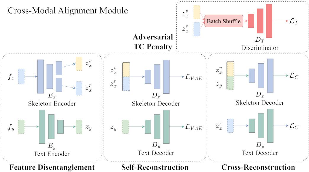
Fig. 3: Cross-Modal Alignment Module. This module serves two primary tasks: latent space construction through self-reconstruction and cross-modal alignment via crossreconstruction. The skeleton features are disentangled into semantic-related ( $z_{x}^{r}$ ) and irrelevant $(z_{x}^{v}$ ) factors.
图 3: 跨模态对齐模块。该模块执行两个主要任务:通过自重构构建潜在空间,以及通过交叉重构实现跨模态对齐。骨架特征被解耦为语义相关 ($z_{x}^{r}$) 和无关 $(z_{x}^{v}$) 因子。
where $\beta_{x}$ and $\beta_{y}$ are hyper parameters, $p_{\theta}(z_{x}^{r})$ , $p_{\theta}(z_{x}^{v})$ , $p_{\theta}(f_{x}|z_{x})$ , $p_{\theta}(z_{y})$ , and $p_{\theta}(f_{y}|z_{y})$ are the probabilities of their presumed distributions, $q_{\phi}(z_{x}|f_{x})$ , $q_{\phi}(z_{x}^{r}|f_{x})$ and $q_{\phi}(z_{x}^{v}|f_{x})$ are the probabilities calculated through our skeleton encoder $E_{x}$ , and $q_{\phi}(z_{y}|f_{y})$ is the one through our text encoder $E_{y}$ . We set the overall VAE loss as
其中 $\beta_{x}$ 和 $\beta_{y}$ 是超参数, $p_{\theta}(z_{x}^{r})$ 、 $p_{\theta}(z_{x}^{v})$ 、 $p_{\theta}(f_{x}|z_{x})$ 、 $p_{\theta}(z_{y})$ 以及 $p_{\theta}(f_{y}|z_{y})$ 是假定分布的概率, $q_{\phi}(z_{x}|f_{x})$ 、 $q_{\phi}(z_{x}^{r}|f_{x})$ 和 $q_{\phi}(z_{x}^{v}|f_{x})$ 是通过我们的骨架编码器 $E_{x}$ 计算出的概率, $q_{\phi}(z_{y}|f_{y})$ 是通过文本编码器 $E_{y}$ 计算出的概率。我们将整体VAE损失设为
$$
\mathcal{L}{V A E}=\mathcal{L}{x}+\mathcal{L}_{y}.
$$
$$
\mathcal{L}{V A E}=\mathcal{L}{x}+\mathcal{L}_{y}.
$$
To better understand our method, we present the $\mathrm{t}$ -SNE visualization of the semantic-related and semantic-irrelevant terms, $z_{x}^{r}$ and $z_{x}^{v}$ in Fig. 4. Figure 4a displays the $\mathrm{t}$ -SNE results for $z_{x}^{r}$ , showing clear class clusters that demonstrate effective disentanglement. In contrast, Figure 4b shows the $\mathrm{t}$ -SNE results for $z_{x}^{v}$ , where class separation is less distinct. This indicates that while our method effectively clusters related semantic features, the irrelevant features remain more dispersed as they contain instance-specific information.
为了更好地理解我们的方法,我们在图4中展示了语义相关项 $z_{x}^{r}$ 和语义无关项 $z_{x}^{v}$ 的 $\mathrm{t}$ -SNE可视化结果。图4a展示了 $z_{x}^{r}$ 的 $\mathrm{t}$ -SNE结果,显示出清晰的类别聚类,表明有效的解耦效果。相比之下,图4b展示了 $z_{x}^{v}$ 的 $\mathrm{t}$ -SNE结果,其类别区分度较低。这表明我们的方法能有效聚类相关语义特征,而无关特征由于包含实例特定信息仍保持较分散状态。
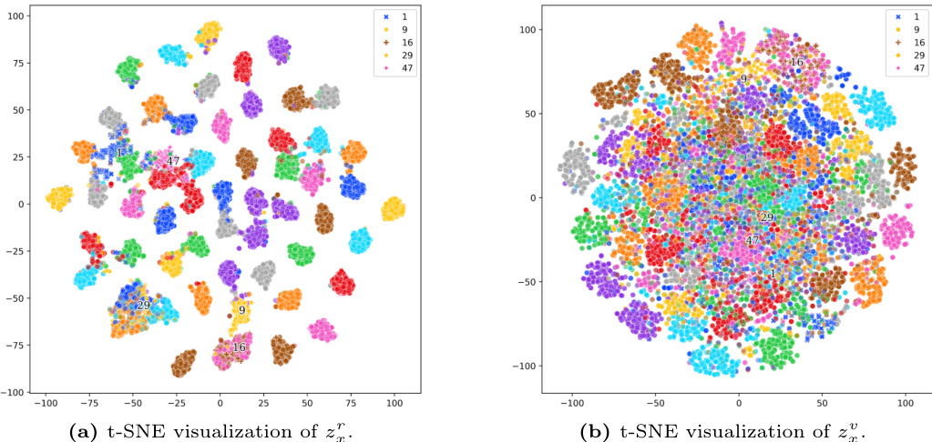
Fig. 4: $\mathrm{t}$ -SNE visualization s of $z_{x}^{\prime}$ and $z_{x}^{v}$ . Best viewed in color.
图 4: $\mathrm{t}$ -SNE 对 $z_{x}^{\prime}$ 和 $z_{x}^{v}$ 的可视化。建议彩色查看。
Cross-Alignment Loss. Because we want our latent text features $z_{y}$ to align with semantic-related skeleton features $z_{x}^{r}$ only, regardless of the semantic-irrelevant features $z_{x}^{v}$ , we regulate them by setting up a cross-alignment loss
交叉对齐损失。我们希望潜在文本特征 $z_{y}$ 仅与语义相关的骨架特征 $z_{x}^{r}$ 对齐,而不受语义无关特征 $z_{x}^{v}$ 的影响,因此通过设置交叉对齐损失进行调控。
$$
\mathcal{L}{C}=|D_{y}(z_{x}^{r})-f_{y}|{2}^{2}+|D_{x}(z_{x}^{v}\oplus z_{y})-f_{x}|_{2}^{2}
$$
$$
\mathcal{L}{C}=|D_{y}(z_{x}^{r})-f_{y}|{2}^{2}+|D_{x}(z_{x}^{v}\oplus z_{y})-f_{x}|_{2}^{2}
$$
to train our VAEs for skeleton and text respectively. This loss enforces skeleton features to be reconstruct able from text features and vice versa. To reconstruct skeleton features from text features, $z_{x}^{v}$ is employed to incorporate necessary style information to mitigate the information gap between the class label and the skeleton sequence.
训练我们的骨架和文本VAE时分别使用。该损失函数强制骨架特征可以从文本特征重建,反之亦然。为了从文本特征重建骨架特征,使用$z_{x}^{v}$来整合必要的风格信息,以缓解类别标签与骨架序列之间的信息差距。
Adversarial Total Correlation Penalty. We expect the features $z_{x}^{r}$ and $z_{x}^{v}$ to be statistically independent, so we impose an adversarial total correlation penalty [3] on them. We train a disc rim in at or $D_{T}$ to predict the probability of a given latent skeleton vector $z_{x}^{v}\oplus z_{x}^{r}$ whether the $z_{x}^{v}$ and $z_{x}^{r}$ come from the same skeleton feature $f_{x}$ . In the ideal case, $D_{T}$ will return $^{1}$ if $z_{x}^{v}$ and $z_{x}^{r}$ are generated together, and $0$ otherwise. To train $D_{T}$ , we design a loss
对抗性总相关惩罚。我们希望特征$z_{x}^{r}$和$z_{x}^{v}$在统计上独立,因此对它们施加了对抗性总相关惩罚[3]。我们训练一个判别器$D_{T}$来预测给定潜在骨架向量$z_{x}^{v}\oplus z_{x}^{r}$的概率,即$z_{x}^{v}$和$z_{x}^{r}$是否来自同一骨架特征$f_{x}$。在理想情况下,如果$z_{x}^{v}$和$z_{x}^{r}$是一起生成的,$D_{T}$将返回$^{1}$,否则返回$0$。为了训练$D_{T}$,我们设计了一个损失函数
$$
\begin{array}{r}{\mathcal{L}{T}=\log D_{T}(z_{x})+\log(1-D_{T}(\tilde{z}_{x})),}\end{array}
$$
$$
\begin{array}{r}{\mathcal{L}{T}=\log D_{T}(z_{x})+\log(1-D_{T}(\tilde{z}_{x})),}\end{array}
$$
where $\tilde{z}{x}$ is an altered feature vector. We create $\tilde{z}{x}$ as the following steps. From a batch of $N$ training samples, our encoder $E_{x}$ generates $N$ pairs of $z_{x,i}^{v}$ and $z_{x,i}^{r}$ , $i=1\ldots N$ . We randomly permute the indices $i$ of $z_{x,i}^{v}$ but keep $z_{x,i}^{r}$ unchanged, and then we concatenate them as $\tilde{z}{x}$ . $D_{T}$ is trained to maximize $L_{T}$ , while $E_{x}$ is adversarial ly trained to minimize it. This training process encourages the encoder to generate latent representations that are independent. Combining the three losses, we set the overall loss
其中 $\tilde{z}{x}$ 是一个经过修改的特征向量。我们通过以下步骤创建 $\tilde{z}{x}$:从包含 $N$ 个训练样本的批次中,编码器 $E_{x}$ 生成 $N$ 对 $z_{x,i}^{v}$ 和 $z_{x,i}^{r}$($i=1\ldots N$)。我们随机置换 $z_{x,i}^{v}$ 的索引 $i$,但保持 $z_{x,i}^{r}$ 不变,然后将它们拼接为 $\tilde{z}{x}$。判别器 $D_{T}$ 被训练以最大化 $L_{T}$,而编码器 $E_{x}$ 则通过对抗训练最小化该损失。这一训练过程促使编码器生成相互独立的潜在表示。结合这三部分损失,我们设定整体损失为
$$
\mathcal{L}=\mathcal{L}{V A E}+\lambda_{1}\mathcal{L}{C}+\lambda_{2}\mathcal{L}_{T},
$$
$$
\mathcal{L}=\mathcal{L}{V A E}+\lambda_{1}\mathcal{L}{C}+\lambda_{2}\mathcal{L}_{T},
$$
where we balance the three losses by hyper parameters $\lambda_{1}$ and $\lambda_{2}$ .
我们通过超参数 $\lambda_{1}$ 和 $\lambda_{2}$ 来平衡这三个损失函数。
Seen, Unseen and Domain Classifier. Because there are two protocols, ZSL and GZSL, to evaluate a zero-shot recognition model, we use two different settings for the two protocols. For the ZSL protocol, we only need to predict the probabilities of classes ${\mathcal{V}}{u}$ from a given skeleton sequence, so we propose a classifier $C_{u}$ as a single-layer MLP (Multilayer Perception) with a softmax output layer yielding the probabilities to predict probabilities of classes ${\mathcal{V}}{u}$ from $z_{y}$ by
可见类、未见类与领域分类器。由于评估零样本识别模型存在ZSL和GZSL两种协议,我们针对这两种协议采用不同设置。对于ZSL协议,只需从给定骨骼序列预测类别${\mathcal{V}}{u}$的概率,因此我们提出一个单层MLP(多层感知器)分类器$C_{u}$,其softmax输出层通过$z_{y}$计算${\mathcal{V}}_{u}$类别的预测概率。
$$
\mathbf{p}{u}=C_{u}(z_{y})=C_{u}(E_{y}(f_{y})),
$$
$$
\mathbf{p}{u}=C_{u}(z_{y})=C_{u}(E_{y}(f_{y})),
$$
where $\mathrm{dim}({\bf p}{u})=|\mathcal{V}{u}|$ . During inference and given an unseen skeleton feature $f_{x}^{u}$ , we get $z_{x}^{u}=E_{x}(f_{x}^{u})$ , separate $z_{x}^{u}$ into zv,u and z $z_{x}^{r,u}$ , and generate $\mathbf{p}{u}=C{u}(z_{x}^{r,u})$ to predict its class as $y_{i}$ and
其中 $\mathrm{dim}({\bf p}{u})=|\mathcal{V}{u}|$。在推理阶段,给定未见过的骨架特征 $f_{x}^{u}$,我们得到 $z_{x}^{u}=E_{x}(f_{x}^{u})$,将 $z_{x}^{u}$ 分离为 $z_{v,u}$ 和 $z_{x}^{r,u}$,并生成 $\mathbf{p}{u}=C_{u}(z_{x}^{r,u})$ 以预测其类别为 $y_{i}$ 且
$$
\hat{i}=\underset{i=1,...,|\mathcal{V}{u}|}{\arg\operatorname*{max}}p_{u}^{i},
$$
$$
\hat{i}=\underset{i=1,...,|\mathcal{V}{u}|}{\arg\operatorname*{max}}p_{u}^{i},
$$
where $p_{u}^{i}$ is the i-th probability value of $\mathbf{p}_{u}$ .
其中 $p_{u}^{i}$ 是 $\mathbf{p}_{u}$ 的第 i 个概率值。
For the GZSL protocol, we need to predict the probabilities of all classes in $\mathcal{V}=\mathcal{V}{u}\cup\mathcal{V}{s}$ where $\mathcal{V}{s}={y_{i}:x_{i}\in\mathcal{X}{s}}$ . We follow the same approach proposed by Gupta et al . [8] to use an additional class classifier $C_{s}$ for seen classes and a domain classifier $C_{d}$ to merge two arrays of probabilities. Gupta et $a l$ . first apply Atzmon and Chechik’s idea [1] to a skeleton-based action recognition problem and outperform the typical single-classifier approach. The advantage of using dual class if i ers is reported in a review paper [19]. Our $C_{s}$ is also a single-layer MLP with a softmax output layer like $C_{u}$ , but it uses skeleton features $f_{x}$ rather than latent features to produce probabilities
对于GZSL协议,我们需要预测$\mathcal{V}=\mathcal{V}{u}\cup\mathcal{V}{s}$中所有类别的概率,其中$\mathcal{V}{s}={y_{i}:x_{i}\in\mathcal{X}{s}}$。我们沿用Gupta等人[8]提出的方法,使用额外的可见类分类器$C_{s}$和域分类器$C_{d}$来合并两个概率数组。Gupta等人首次将Atzmon和Chechik的思想[1]应用于基于骨架的动作识别问题,其性能超越了典型的单分类器方法。双分类器的优势已在综述论文[19]中得到验证。我们的$C_{s}$与$C_{u}$类似,也是带有softmax输出层的单层MLP,但使用骨架特征$f_{x}$而非潜在特征来生成概率。
$$
\mathbf{p}{s}=C_{s}(f_{x}),
$$
$$
\mathbf{p}{s}=C_{s}(f_{x}),
$$
where $\mathrm{dim}(\mathbf{p}{s})=|\mathcal{V}_{s}|$ .
其中 $\mathrm{dim}(\mathbf{p}{s})=|\mathcal{V}_{s}|$。
We train $C_{s}$ and $C_{u}$ first, and then we freeze their parameters to train $C_{d}$ , which is a logistic regression with an input vector $\mathbf{p}{s}^{\prime}\oplus\mathbf{p}{u}$ where ${\bf p}{s}^{\prime}$ is the temperature-tuned [10] top $k$ -pooling result of $\mathbf{p}{s}$ and the number $k=\dim({\bf p}{u})$ . $C_{d}$ yields a probability value $p_{d}$ of whether the source skeleton belongs to a seen class. We use the LBFGS algorithm [16] to train $C_{d}$ and use it during inference to predict the probability of $x$ as
我们首先训练 $C_{s}$ 和 $C_{u}$,然后冻结它们的参数来训练 $C_{d}$。$C_{d}$ 是一个逻辑回归模型,其输入向量为 $\mathbf{p}{s}^{\prime}\oplus\mathbf{p}{u}$,其中 ${\bf p}{s}^{\prime}$ 是 $\mathbf{p}{s}$ 经过温度调节 [10] 后的 top $k$ 池化结果,且 $k=\dim({\bf p}{u})$。$C_{d}$ 输出一个概率值 $p_{d}$,表示源骨架是否属于已见过的类别。我们使用 LBFGS 算法 [16] 训练 $C_{d}$,并在推理时用它来预测 $x$ 的概率为
$$
\mathbf{p}(y|x)=C_{d}(\mathbf{p}{s}^{\prime}\oplus\mathbf{p}{u})\mathbf{p}{s}\oplus(1-C_{d}(\mathbf{p}{s}^{\prime}\oplus\mathbf{p}{u}))\mathbf{p}{u}=p_{d}\mathbf{p}{s}\oplus(1-p_{d})\mathbf{p}_{u}
$$
$$
\mathbf{p}(y|x)=C_{d}(\mathbf{p}{s}^{\prime}\oplus\mathbf{p}{u})\mathbf{p}{s}\oplus(1-C_{d}(\mathbf{p}{s}^{\prime}\oplus\mathbf{p}{u}))\mathbf{p}{u}=p_{d}\mathbf{p}{s}\oplus(1-p_{d})\mathbf{p}_{u}
$$
and decide the class of $x$ as $y_{i}$ and
并将 $x$ 的类别判定为 $y_{i}$
$$
\hat{i}=\underset{i=1,\ldots,|y|}{\arg\operatorname*{max}}p^{i},
$$
$$
\hat{i}=\underset{i=1,\ldots,|y|}{\arg\operatorname*{max}}p^{i},
$$
where $p^{i}$ is the i-th probability value of ${\bf p}(y\vert x)$ .
其中 $p^{i}$ 是 ${\bf p}(y\vert x)$ 的第 i 个概率值。
4 Experiments
4 实验
Datasets. We conduct experiments on three datasets and show their statistics in Table 1. We adopt the cross-subject split, where half of the subjects are used for training and the other half for validation. We use NTU-60 and NTU120 as synonyms for the NTU RGB+D and NTU RGB+D 120 datasets. Due to discrepancies in class labels between the official website5 and the GitHub codebase $^6$ of NTU-60 and NTU-120 datasets (e.g. the label of class 18 is “put on glasses” in their website but “wear on glasses” in GitHub), we follow existing methods by using the class labels provided in their codebase.
数据集。我们在三个数据集上进行实验,统计数据如表 1 所示。采用跨受试者划分方式,其中一半受试者用于训练,另一半用于验证。NTU-60 和 NTU120 是 NTU RGB+D 与 NTU RGB+D 120 数据集的同义词。由于 NTU-60 和 NTU-120 数据集在官网5与 GitHub 代码库6的类别标签存在差异(例如类别 18 的标签在官网为 "put on glasses" 而在 GitHub 为 "wear on glasses"),我们遵循现有方法采用其代码库提供的类别标签。
Table 1: Statistics of datasets used in our experiments
表 1: 实验所用数据集统计
| Name | Class | Subject | Joint Sample | Camera View |
|---|---|---|---|---|
| NTURGB+D [23] | 40 | 25 | 56,880 | 3 |
| NTU RGB+D 120 [17] | 120 | 106 | 114,480 | 3 |
| PKU-MMD [5] | 66 | 25 | 28,443 | 3 |
Implementation Details. We implement the disc rim in at or $D_{T}$ as a two-layer MLP with ReLU activation and a Sigmoid output layer, and the encoders $E_{x}$ , $E_{y}$ , decoders $D_{x}$ , $D_{y}$ , seen and unseen class if i ers $C_{s}$ , $C_{u}$ as single-layer MLPs. During training, we alternatively train VAEs and $D_{T}$ . We train VAEs first, and after training VAEs $n_{d}$ times, we train $D_{T}$ once.
实现细节。我们将判别器 $D_{T}$ 实现为带有ReLU激活函数和Sigmoid输出层的两层MLP,编码器 $E_{x}$、$E_{y}$,解码器 $D_{x}$、$D_{y}$,以及可见类和未见类分类器 $C_{s}$、$C_{u}$ 则实现为单层MLP。训练过程中,我们交替训练VAE和 $D_{T}$:先训练VAE $n_{d}$ 次,再训练一次 $D_{T}$。
We use the LBFGS implementation from Scikit-learn [18] to train $C_{d}$ and divide our training set into a validation seen set and a validation unseen set. As the training of $C_{d}$ requires seen and unseen skeleton features $(f_{x}^{s},f_{x}^{u})$ , we re-train other components using the validation seen set and use the validation unseen set to provide unseen skeleton features to train $C_{d}$ . Finally, the trained $C_{d}$ is used to make inferences on the testing set. The number of classes in the validation unseen set is the same as the original unseen class set $|\mathcal{V}_{u}|$ .
我们使用Scikit-learn [18]中的LBFGS实现来训练$C_{d}$,并将训练集划分为验证可见集和验证未见集。由于$C_{d}$的训练需要可见和未见骨架特征$(f_{x}^{s},f_{x}^{u})$,我们使用验证可见集重新训练其他组件,并通过验证未见集提供未见骨架特征来训练$C_{d}$。最终,训练好的$C_{d}$用于在测试集上进行推断。验证未见集中的类别数量与原始未见类别集$|\mathcal{V}_{u}|$相同。
We use the cyclical annealing schedule [7] to train our VAEs because cyclical annealing mitigates the KL divergence vanishing problem. At the beginning of each epoch, we set the actual training hyper parameters $\lambda_{2}^{\prime}$ , $\beta_{1}^{\prime}$ , and $\beta_{2}^{\prime}$ as $0$ until we use one-third training samples. Thereafter, we progressively increase $\lambda_{2}^{\prime}$ , $\beta_{1}^{\prime}$ , and $\beta_{2}^{\prime}$ to $\lambda_{2}$ , $\beta_{x}$ , and $\beta_{y}$ based on the number of trained samples, e.g,
我们采用周期性退火策略 [7] 来训练变分自编码器 (VAE),因为周期性退火能缓解KL散度消失问题。在每个训练周期开始时,我们将实际训练超参数 $\lambda_{2}^{\prime}$、$\beta_{1}^{\prime}$ 和 $\beta_{2}^{\prime}$ 设为 $0$,直到使用三分之一训练样本为止。之后,根据已训练样本数量,我们逐步将 $\lambda_{2}^{\prime}$、$\beta_{1}^{\prime}$ 和 $\beta_{2}^{\prime}$ 提升至 $\lambda_{2}$、$\beta_{x}$ 和 $\beta_{y}$。例如,
where $k$ and $n$ are the index and total number of training samples in an epoch. We set $\lambda_{1}$ as $0$ in our first epoch and 1 for all subsequent epochs. We conduct our experiments on a machine equipped with an Intel i7-13700 CPU, an NVIDIA RTX 3090 GPU, and 32GB RAM. We implement our method using PyTorch 2.1.0, scikit-learn 1.3.2, and scipy 1.11.3. It takes 4.6 hours to train our model for a 55/5 split of the NTU RGB+D 60 dataset, and 8.7 hours for a 110/10 split of the NTU RGB+D 120 dataset. We determine the hyper parameters through random search, as listed in Tables 2 and 5. The hyper parameter search space is detailed in Supplementary Materials Section A.
其中 $k$ 和 $n$ 分别表示一个训练周期中样本的索引和总数。我们将第一周期的 $\lambda_{1}$ 设为 $0$ ,后续所有周期设为 1。实验在一台配备 Intel i7-13700 CPU、NVIDIA RTX 3090 GPU 和 32GB 内存的机器上进行,采用 PyTorch 2.1.0、scikit-learn 1.3.2 和 scipy 1.11.3 实现。在 NTU RGB+D 60 数据集 55/5 划分方案下训练耗时 4.6 小时,NTU RGB+D 120 数据集 110/10 划分方案下耗时 8.7 小时。超参数通过随机搜索确定,具体数值见表 2 和表 5,搜索空间详见补充材料 A 节。
Table 2: Setting for comparison with existing methods.
表 2: 与现有方法对比的实验设置
| NTU-60 | NTU-120 |
|---|---|
| SkeletonFeatureExtractor TextFeatureExtractor | Shift-GCN [4] Sentence-BERT [21] |
| Epochs Optimizer | 10 Adam |
| Optimizer Momentum | β1 = 0.9,β2 = 0.999 |
| Batch size | 32 |
| Learning rate | 3.39e-05 3.48e-05 |
| Weights of DkL in LvAE | βx =0.023,βy = 0.011 |
| Weight of LT | 入2 = 0.011 |
| Discriminator steps nd | 5 4 |
| Hidden dim. of zr and zy | 160 256 |
| Hidden dim. of z2 | 8 32 |
Table 3: ZSL accuracy ( $%$ ) on the NTU RGB+D datasets.
表 3: NTU RGB+D 数据集上的零样本学习 (ZSL) 准确率 ( $%$ )
| 方法 | NTU-60 | NTU-120 |
|---|---|---|
| 17.49 | 1 0 1 1 1 | |
| ReViSE [13] | 53.91 | 55.04 32.38 |
| JPoSE [25] CADA-VAE [22] | 64.82 28.75 76.84 | 51.93 32.44 |
| SynSE [8] | 28.96 75.81 | 59.53 35.77 |
| SMIE [29] | 33.30 77.98 40.18 | 62.69 38.70 65.74 45.30 |
| SA-DVAE | 82.37 41.38 | 68.77 46.12 |
Comparison with SOTA methods. We compare our method with several state-of-the-art zero-shot action recognition methods using the setting shown in Table 2 and report their results in Tables 3 and 4. We use the same feature extractors and class splits as the one used by SynSE, and the only difference lies in the network architecture.
与SOTA方法的对比。我们使用表2所示的设置,将我们的方法与几种最先进的零样本动作识别方法进行比较,并在表3和表4中报告它们的结果。我们使用了与SynSE相同的特征提取器和类别划分,唯一的区别在于网络架构。
The results show that SA-DVAE works well, in particular for unseen classes. Furthermore, for the more challenging GZSL task, SA-DVAE even improves more over existing methods. On the NTU RGB+D 60 dataset, SA-DVAE improves the accuracy of $(+7.25%$ and $+6.23%$ ) in the GZSL protocol, greater than the $(+4.39%$ and $+1.2%$ ) in the ZSL one.
结果表明,SA-DVAE表现良好,尤其对于未见过的类别。此外,在更具挑战性的GZSL任务中,SA-DVAE相比现有方法提升更为显著。在NTU RGB+D 60数据集上,SA-DVAE在GZSL协议中将准确率提高了$(+7.25%$和$+6.23%),高于ZSL协议中的$(+4.39%$和$+1.2%)。
Random Class Splits and Improved Feature Extractors. The setting of class splits is crucial for accuracy calculation and Tables 3 and 4 only show results of a few predefined splits, which can not infer the overall performance on a complete dataset. Thus, we follow Zhou et al.’s approach [29] to randomly select several unseen classes as a new split, repeat it three times, and report the average performance. In addition, we use improved skeleton feature extractor ST-GCN [26] and text extractor CLIP [20], chosen for their broad applicability and robust performance across different domains. We also tested different feature extractors, which can be found in Supplementary Materials Section B.
随机类别划分与改进的特征提取器。类别划分的设置对准确率计算至关重要,表3和表4仅展示了几种预定义划分的结果,无法推断模型在完整数据集上的整体表现。因此,我们采用Zhou等人[29]的方法,随机选择若干未见类别作为新划分,重复三次并报告平均性能。此外,我们选用具有广泛适用性和跨领域稳健表现的改进骨架特征提取器ST-GCN[26]及文本提取器CLIP[20]。其他特征提取器的测试结果详见补充材料B章节。
Table 4: GZSL metrics: seen class accuracy $A c c_{s}$ , unseen class accuracy $A c c_{u}$ , and their harmonic mean $H(%)$ on the NTU RGB+D datasets. *: SynSE paper reports 29.22, but it is a miscalculation.
表 4: GZSL指标: 可见类准确率 $A c c_{s}$ 、不可见类准确率 $A c c_{u}$ 及其调和平均数 $H(%)$ 在NTU RGB+D数据集上的表现。*: SynSE论文报告值为29.22,但这是计算错误。
| Method | NTU-60 | NTU-120 | ||
|---|---|---|---|---|
| 55/5 split | 48/12 split | 110/10 split | 96/24 split | |
| Accs AcCu H | Accs AcCu H | Accs AcCu H | Accs AcCu H | |
| ReViSE [13] | 74.22 34.73 347.32* | 62.36 20.77 31.16 | 48.69 44.84 46.68 | 49.66 25.06 33.31 |
| JPoSE [25] | 64.44 50.29 56.49 | 60.49 20.62 30.75 | 47.66 46.40 47.05 | 538.62 22.79 28.67 |
| CADA-VAE[22] | 69.38 61.79 65.37 | 51.32 27.03 35.41 | 47.16 49.78 48.44 | 41.11 34.14 137.31 |
| SynSE [8] | 61.27 56.93 59.02 | 52.21 27.85 36.33 | 52.51 57.60 54.94 | 56.39 32.25 41.04 |
| SA-DVAE | 62.28 70.80 66.27 | 50.20 36.94 42.56 | 61.10 59.75 60.42 | 58.82 35.79 44.50 |
Table 5: Settings for the random-split experiment.
表 5: 随机分割实验的设置。
| NTU-60 | NTU-120 | PKU-MMD | |
|---|---|---|---|
| SkeletonFeatureExtractor | ST-GCN [26] | ||
| TextFeatureExtractor | CLIP-ViT-B/32 [20] | ||
| Epochs | 10 | ||
| Optimizer | Adam | ||
| No. of unseen classes | 5 | 10 | 5 |
| OptimizerMomentum | β1 = 0.9, β2 = 0.999 | ||
| Batch size | 32 | 32 | 64 |
| Learning rate | 3.60e-05 | 7.36e-5 | 3.07e-05 |
| Weights of DkL in LvAE | βx = 0.023, βy = 0.011 | ||
| Weight of LT | λ2 = 0.011 | ||
| Discriminator steps nd | 7 | 12 | 2 |
| Hidden dim. of zr and zy | 224 | 176 | 128 |
| Hidden dim. of z | 16 | 20 | 16 |
Table 5 shows our settings and Tables 6 and 7 show the results, where naive alignment means that we disable $D_{T}$ and remove the extra head for $z_{x}^{v}$ , and FD means that we disable $D_{T}$ . The results show that both feature disentanglement and total correlation penalty contribute to accuracy improvements, and feature disentanglement is the major contributor, e.g., $+12.95%$ on NTU-60 compared to naive alignment in Table 6. The adversarial total correlation penalty (TC) slightly reduces the accuracy for seen classes but significantly improves unseen and overall accuracy. This is because TC enhances the embedding quality by reducing feature redundancy, making the domain classifier less biased towards seen classes. Consequently leading to improved generalization. The results in Tab. 7 highlight this trade-off, where the improved harmonic mean indicates a more balanced and robust performance across both seen and unseen classes.
表5展示了我们的设置,表6和表7则呈现了实验结果。其中,朴素对齐(naive alignment)表示我们禁用了$D_{T}$并移除了$z_{x}^{v}$的额外头部,FD表示我们禁用了$D_{T}$。结果表明,特征解耦(feature disentanglement)和总相关惩罚(total correlation penalty)都对精度提升有所贡献,且特征解耦是主要贡献因素,例如在表6中NTU-60数据集上相比朴素对齐提升了$+12.95%$。对抗性总相关惩罚(TC)略微降低了已见类别的准确率,但显著提升了未见类别和整体准确率。这是因为TC通过减少特征冗余提升了嵌入质量,使得领域分类器对已见类别的偏向性降低,从而改善了泛化能力。表7的结果凸显了这种权衡关系,其中提升的调和平均数(harmonic mean)表明模型在已见和未见类别上取得了更均衡、更鲁棒的性能。
Table 6: Average ZSL accuracy ( $%$ ) under the random split setting on the NTU60, NTU-120, and PKU-MMD datasets. FD: feature disentanglement. TC: adversarial total correlation penalty. †: PoS tags for the PKU-MMD dataset are obtained from spaCy [12].
表 6: NTU60、NTU-120和PKU-MMD数据集在随机划分设置下的平均零样本学习(ZSL)准确率( $%$ )。FD: 特征解耦。TC: 对抗性总相关惩罚。†: PKU-MMD数据集的词性标注(PoS tags)来自spaCy [12]。
| 方法 | NTU-60 NTU-120 55/5划分 110/10划分 | PKU-MMD 46/5划分 |
|---|---|---|
| ReViSE [13] | 60.94 44.90 | 59.34 |
| JPoSEt [25] | 59.44 46.69 | 57.17 |
| CADA-VAE [22] | 61.84 45.15 | 60.74 |
| SynSE+ [8] | 64.19 47.28 | 53.85 |
| SMIE [29] | 65.08 46.40 | 60.83 |
| Naive alignment | 69.26 39.73 | 60.13 |
| FD | 82.21 49.18 | 60.97 |
| SA-DVAE C (FD+TC) | 84.20 50.67 | 66.54 |
Table 7: Average GZSL metrics: seen class accuracy $A c c_{s}$ , unseen class accuracy $A c c_{u}$ , and their harmonic mean $H(%)$ under the random split setting on the NTU-60, NTU120, and PKU-MMD datasets. FD: feature disentanglement. TC: adversarial total correlation penalty. $^\dagger$ : PoS tags for the PKU-MMD dataset are obtained from spaCy [12].
表 7: 在NTU-60、NTU120和PKU-MMD数据集随机划分设置下的平均广义零样本学习(GZSL)指标:可见类准确率$Acc_{s}$、不可见类准确率$Acc_{u}$及其调和均值$H(%)$。FD:特征解耦。TC:对抗性总相关惩罚。$^\dagger$:PKU-MMD数据集的词性标注(PoS tags)来自spaCy [12]。
| 方法 | NTU-60 55/5划分 | NTU-120 110/10划分 | PKU-MMD 46/5划分 | |||
|---|---|---|---|---|---|---|
| Accs AcCu | H | Accs AcCu | H | Accs AcCu | H | |
| ReViSE [13] | 71.75 52.06 | 60.34 | 48.29 34.64 | 40.34 | 60.89 42.16 | 49.82 |
| JPoSE + [25] | 66.25 54.92 | 60.05 | 49.43 39.14 | 43.69 | 60.26 45.18 | 51.64 |
| CADA-VAE [22] | 77.35 58.14 | 66.38 | 51.09 41.24 | 45.64 | 63.17 35.86 | 45.75 |
| SynSE + [8] | 75.84 60.77 | 67.47 | 41.73 45.36 | 43.47 | 63.09 40.69 | 49.47 |
| Naivealignment | 82.11 47.99 | 60.58 | 57.01 31.62 | 40.68 | 58.76 43.14 | 49.75 |
| FD | 82.31 61.98 | 370.71 | 58.57 37.83 | 45.97 | 58.11 48.15 | 52.66 |
| SA-DVAE (FD+TC) | 78.16 72.60 | 75.27 | 58.09 40.23 | 47.54 | 58.49 51.40 | 54.72 |
From our three runs of the random-split experiment on the NTU-60 dataset (average results is shown in Table 6), we pick the most challenging run and show its per-class accuracy in Fig. 5 and the t-SNE visualization of skeleton features ( $f_{x}$ ) in Fig. 6. The labels of classes 16 and 17 are “wear a shoe” and “take off a shoe” and their movements are acted as a person sitting on a chair who bends down her upper body and stretches her arm to touch her shoe. The skeleton sequences of the two classes are highly similar so are their extracted features. In Fig. 6, samples of classes 16 and 17 are overlapped, and naive alignment generates poor accuracy on class 16. Similarly, naive alignment generates nearzero accuracy on classes 9 and 29. Since both classes 9 and 16 share similar skeleton sequences and were unseen during training, their features appear highly similar. This similarity leads naive alignment to mis classify samples belonging to class 9 as class 16. We can see significant improvements with the addition of FD and TC. These techniques allow the model to prioritize semantic-related information and improve classification performance.
我们在NTU-60数据集上进行了三次随机分割实验(平均结果如表6所示),选取最具挑战性的一次运行结果展示其每类准确率(图5)及骨架特征( $f_{x}$ )的t-SNE可视化(图6)。类别16和17的标签分别为"穿鞋"和"脱鞋",其动作表现为人坐在椅子上俯身伸手触鞋。这两类的骨架序列高度相似,提取的特征也极为接近。图6显示类别16和17的样本存在重叠,朴素对齐方法在类别16上准确率极低。同理,该方法在类别9和29上的准确率近乎为零。由于类别9与16的骨架序列相似且训练时未出现,它们的特征表现出高度相似性,导致朴素对齐将类别9样本误判为类别16。通过引入FD(特征解耦)和TC(时间对比)技术,分类性能得到显著提升,这些技术使模型能聚焦语义相关信息。

Fig. 5: Unseen per-class accuracy of the NTU-60 dataset. The unseen split {1, 9, 16, 29, 47} is used in a challenging run of our random-split GZSL experiments.
图 5: NTU-60数据集的未见类别准确率。在我们的随机分割广义零样本学习(GZSL)实验的挑战性测试中,使用了未见分割{1, 9, 16, 29, 47}。
Table 8: Average GZSL metrics ( $%$ ) of different seen classifier input under the random split setting on the NTU-60, NTU-120, and PKU-MMD datasets.
表 8: 不同可见分类器输入在NTU-60、NTU-120和PKU-MMD数据集随机划分设置下的平均广义零样本学习(GZSL)指标( $%$ )。
| 方法 | NTU-60 55/5划分 | NTU-120 110/10划分 | PKU-MMD 46/5划分 |
|---|---|---|---|
| Accs AcCu | H | Accs AcCu | |
| SA-DVAE (2作为输入) | 72.00 71.48 | 71.74 | 55.35 39.00 |
| SA-DVAE (fx作为输入) | 78.16 72.60 | 75.27 | 58.09 40.23 47.54 58.49 51.40 54.72 |
Impact of Replacing Skeleton Feature $f_{x}$ with Semantic-Related Latent Vector $z_{x}^{r}$ in Seen Classifier We replace the input skeleton feature $f_{x}$ of the seen classifier with the disentangled semantic-related latent vector $z_{x}^{r}$ under the random-split setting listed in Tab. 5 and report results in Tab. 8. Notably, since the semantic-irrelevant terms also contain information that is beneficial for classification but not necessary related to the text descriptions, $f_{x}$ retains both semantic-related and irrelevant details. This dual retention enhances performance compared to $z_{x}^{r}$ , which focuses solely on semantic-related information.
用语义相关隐向量 $z_{x}^{r}$ 替换骨架特征 $f_{x}$ 对可见分类器的影响
在表5所列的随机划分设置下,我们将可见分类器的输入骨架特征 $f_{x}$ 替换为解耦的语义相关隐向量 $z_{x}^{r}$ ,结果如表8所示。值得注意的是,由于语义无关项也包含对分类有益但与文本描述非必要关联的信息, $f_{x}$ 同时保留了语义相关和无关的细节。这种双重保留使得其性能优于仅聚焦语义相关信息的 $z_{x}^{r}$ 。
We incorporate zero-shot learning and action recognition techniques, including pose canonical iz ation [11] and enhanced action descriptions [29], with additional experimental results in Supplementary Materials Section C.
我们结合了零样本 (zero-shot) 学习和动作识别技术,包括姿态规范化 (pose canonicalization) [11] 和增强动作描述 (enhanced action descriptions) [29],并在补充材料C部分提供了更多实验结果。

Fig. 6: $\mathrm{t}$ -SNE visualization of $f_{x}$ of the NTU-60 dataset. The unseen split is used in a run of our random-split GZSL experiments. Best viewed in color.
图 6: NTU-60 数据集 $f_{x}$ 的 $\mathrm{t}$-SNE 可视化。在我们的随机分割广义零样本学习 (GZSL) 实验中使用了未见过的分割 。建议彩色查看。
5 Conclusion
5 结论
ZSL study aims to leverage knowledge from one domain to help solve problems in another domain and has been proven useful for action recognition tasks, in particular for 3D skeleton data because it is expensive and labor-consuming to build accurately labeled datasets. Although there are several existing methods in the literature, they never address the asymmetry problem between skeleton data and text description. In this paper, we propose SA-DVAE, a cross-modality alignment model using the feature disentanglement approach to differentiate skeleton data into two independent representations, the semantic-related and irrelevant ones. Along with an adversarial disc rim in at or to enhance the feature disentanglement, our experiments show that the proposed method generates better performance over existing methods on three benchmark datasets in both ZSL and GZSL protocols.
零样本学习 (ZSL) 研究旨在利用一个领域的知识帮助解决另一个领域的问题,并已被证明对动作识别任务特别有用,尤其是针对3D骨骼数据,因为构建精确标注的数据集成本高昂且耗时。尽管文献中存在多种现有方法,但它们从未解决骨骼数据与文本描述之间的不对称性问题。本文提出SA-DVAE,这是一种跨模态对齐模型,采用特征解耦方法将骨骼数据分解为两个独立表示:语义相关和语义无关。通过引入对抗判别器来增强特征解耦,实验表明,在零样本学习和广义零样本学习 (GZSL) 协议下,所提方法在三个基准数据集上的性能优于现有方法。