TS-SEP: Joint Di ari z ation and Separation Conditioned on Estimated Speaker Embeddings
TS-SEP:基于估计说话人嵌入的联合二值化与分离
Christoph Boeddeker, Aswin Shanmugam Subramania n, Gordon Wichern, Reinhold Haeb-Umbach, and Jonathan Le Roux
Christoph Boeddeker、Aswin Shanmugam Subramanian、Gordon Wichern、Reinhold Haeb-Umbach 和 Jonathan Le Roux
Abstract—Since di ari z ation and source separation of meeting data are closely related tasks, we here propose an approach to perform the two objectives jointly. It builds upon the targetspeaker voice activity detection (TS-VAD) di ari z ation approach, which assumes that initial speaker embeddings are available. We replace the final combined speaker activity estimation network of TS-VAD with a network that produces speaker activity estimates at a time-frequency resolution. Those act as masks for source extraction, either via masking or via beam forming. The technique can be applied both for single-channel and multi-channel input and, in both cases, achieves a new state-of-the-art word error rate (WER) on the LibriCSS meeting data recognition task. We further compute speaker-aware and speaker-agnostic WERs to isolate the contribution of di ari z ation errors to the overall WER performance.
摘要:由于会议数据的说话人日志化(diarization)和源分离是密切相关的任务,我们在此提出一种联合实现这两个目标的方法。该方法基于目标说话人语音活动检测(TS-VAD)的说话人日志化方案,该方案假设初始说话人嵌入是可用的。我们将TS-VAD最终组合的说话人活动估计网络替换为一个能在时频分辨率下生成说话人活动估计的网络。这些估计通过掩蔽或波束成形作为源提取的掩码。该技术可同时应用于单通道和多通道输入,在这两种情况下都在LibriCSS会议数据识别任务上实现了最新的词错误率(WER)最优水平。我们进一步计算了说话人相关和说话人无关的WER,以分离说话人日志化错误对整体WER性能的贡献。
Index Terms—Meeting recognition, meeting separation, speaker di ari z ation
索引术语—会议识别、会议分离、说话人日志
I. INTRODUCTION
I. 引言
URRENT research in meeting transcription is not only concerned with transcribing the audio recordings of meetings into machine-readable text, but also with enriching the transcription with di ari z ation information about “who spoke when”. Much of the difficulty of these two tasks can be attributed to the interaction dynamics of multi-talker conversational speech. Speakers articulate themselves in an intermittent manner with alternating segments of speech inactivity, singletalker speech, and multi-talker speech. In particular, overlapping speech, where two or more people are talking at the same time, is known to pose a significant challenge not only to ASR but also to di ari z ation [1].
当前会议转录的研究不仅关注将会议录音转写为机器可读文本,还致力于通过添加"谁在何时发言"的说话人日志(diarization)信息来丰富转录内容。这两项任务的主要难点源于多人对话语音的交互动态特性:发言者以间歇方式表达,交替出现静默、单人发言和多人同时发言的片段。特别是重叠语音(即两人或多人同时说话)现象,已知会对自动语音识别(ASR)和说话人日志[1]都构成重大挑战。
There is no obvious choice whether to start the processing with a di ari z ation or with a separation/enhancement module [2]. An argument in favor of first separating the overlapped speech segments, and at the same time removing other acoustic distortions, and then carrying out di ari z ation, is the fact that the di ari z ation task is much easier when performed on speech without overlap. This processing order was advocated in [2]. Also, the continuous speech separation (CSS) pipeline starts with a separation module [3]. Early di ari z ation systems, such as the clustering-based approaches that were predominant in
在处理流程中,是优先进行说话人日志化 (diarization) 还是先进行分离/增强模块 [2],并没有一个明确的选择。支持先分离重叠语音段,同时去除其他声学失真,再进行说话人日志化的观点认为,当处理没有重叠的语音时,说话人日志化任务会简单得多。[2] 中提倡了这一处理顺序。此外,连续语音分离 (CSS) 流程也是从分离模块开始的 [3]。早期的说话人日志化系统,如当时主流的基于聚类的方法...
C. Boeddeker and R. Haeb-Umbach are with Paderborn University, Paderborn, 33098, Germany (e-mail: {boeddeker,haeb}@nt.upb.de). A. S. Subramania n was with Mitsubishi Electric Research Laboratories (MERL), Cambridge, MA 02139, USA, and is now with Microsoft Corporation, One Microsoft Way, Redmond, WA 98052, USA (e-mail: asubra $13\ @$ alumni.jh.edu). G. Wichern and J. Le Roux are with Mitsubishi Electric Research Laboratories (MERL), Cambridge, MA 02139, USA (e-mail: {wichern,leroux}@merl.com).
C. Boeddeker 和 R. Haeb-Umbach 就职于德国 33098 帕德博恩大学帕德博恩分校 (邮箱: {boeddeker,haeb}@nt.upb.de)。A. S. Subramanian 曾就职于美国马萨诸塞州剑桥市 02139 三菱电机研究实验室 (MERL),现就职于美国华盛顿州雷德蒙市 98052 微软大道一号微软公司 (邮箱: asubra$13\ @$alumni.jh.edu)。G. Wichern 和 J. Le Roux 就职于美国马萨诸塞州剑桥市 02139 三菱电机研究实验室 (MERL) (邮箱: {wichern,leroux}@merl.com)。
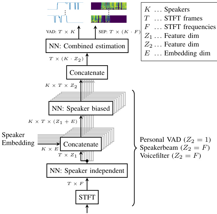
Fig. 1. TS-VAD and TS-SEP structure for one microphone. Speakers indicated as “shading”.
图 1: 单麦克风的 TS-VAD 和 TS-SEP 结构。说话人用"阴影"表示。
the first editions of the DiHARD di ari z ation challenge, were generally unable to properly cope with overlapping speech, and thus performed poorly on data with a significant amount of concurrent speech [4].
DiHARD语音分离挑战赛的前几届版本通常无法有效处理重叠语音,因此在存在大量并发语音的数据上表现不佳 [4]。
On the other hand, starting the processing with the diarization component can be advantageous, because signal extraction is eased if information about the segment boundaries of speech absence, single-, and multi-talker speech is given. This order of processing has for example been adopted in the CHiME6 baseline system [1]. However, this requires the di ari z ation component to be able to cope with overlapped speech.
另一方面,先进行说话人日志(diarization)处理具有优势,因为若已知语音静默段、单人说话段和多人重叠说话段的边界信息,信号提取会更容易。这种处理顺序已被CHiME6基线系统[1]采用,但要求说话人日志组件能够处理重叠语音。
These different points of view highlight the interdependence of the two tasks, and they are a clear indication that a joint treatment of di ari z ation and separation/source extraction can be beneficial. Indeed, subtasks to be solved in either of the two are similar: while di ari z ation is tasked with determining the speakers that are active in each time frame, mask-based source extraction in essence identifies the active speakers for each time-frequency (TF) bin, the difference thus being only the resolution, time vs. time-frequency.
这些不同观点凸显了两项任务的相互依存性,也明确表明将说话人日志化(diarization)与分离/源提取进行联合处理可能带来益处。事实上,两个子任务需要解决的环节具有相似性:说话人日志化需要确定每个时间帧中的活跃说话人,而基于掩码的源提取本质上识别的是每个时频(TF)单元中的活跃说话人,两者的区别仅在于分辨率不同(时间维度 vs. 时频维度)。
Early examples of joint di ari z ation and source separation systems are spatial mixture models (SMMs) using timevarying mixture weights [5], [6]. There, the estimates of the prior probabilities of the mixture components, after appropriate quantization, give the di ari z ation information about who speaks when, while the posterior probabilities have TFresolution and can be employed to extract each source present in a mixture, either by masking or by beam forming. A crucial issue is the initialization of the mixture weights or posterior probabilities. In the guided source separation (GSS) framework [7], which was part of the baseline system of the CHiME6 challenge [1], manual annotation of the segment boundaries, and later estimates thereof [8], were used to initialize the timevarying mixture weights. An initialization scheme exploiting the specifics of meeting data, in which most of the time only a single speaker is active, was introduced in [6].
联合说话人日志和源分离系统的早期例子是使用时变混合权重的空间混合模型 (SMM) [5], [6]。其中,混合分量先验概率的估计经过适当量化后可提供"谁在何时说话"的日志信息,而后验概率具有时频分辨率,可通过掩蔽或波束成形来提取混合信号中的各个声源。关键问题在于混合权重或后验概率的初始化。在CHiME6挑战赛基线系统[1]采用的引导源分离(GSS)框架[7]中,最初使用人工标注的片段边界[8]来初始化时变混合权重。文献[6]提出了一种针对会议数据特性的初始化方案,该场景下多数时间只有单个说话人处于活跃状态。
However, this approach to joint di ari z ation and separation depends on the availability of multi-channel input, and, due to the iterative nature of the expectation maximization (EM) algorithm, it is computationally demanding. Furthermore, the EM algorithm is, at least in its original formulation, an offline algorithm that is not well suited for processing arbitrarily long meetings. There exist recursive online variants of the EM algorithm, which are nevertheless computationally intense and need careful parameter tuning, in particular in dynamic scenarios [9].
然而,这种联合对角化和分离的方法依赖于多通道输入的可用性,并且由于期望最大化 (EM) 算法的迭代特性,其计算需求较高。此外,EM 算法至少在其原始形式中是一种离线算法,不太适合处理任意长度的会议。虽然存在递归的在线 EM 算法变体,但它们计算量仍然很大,并且需要仔细调整参数,特别是在动态场景中 [9]。
In light of their recent success, both in di ari z ation and source separation, neural networks appear to be promising for developing an integrated solution to the problem of joint di ari z ation and separation/extraction. Well-known methods for extracting a target speaker from a mixture include SpeakerBeam [10] and Voice Filter [11]. Both require an enrollment utterance of the target speaker to be extracted. In the Speaker Beam approach, the target speaker embedding and the extraction network are trained jointly, while Voice Filter employs a separately trained speaker embedding computation network. However, their reliance on the availability of an enrollment sentence somewhat limits their usefulness for some applications. Furthermore, they have been designed for a typical source separation/extraction scenario, where it is a priori known that the target speaker is active most of the time. Only recently has an extension of the Speaker Beam system been proposed, to deal with meeting data [12].
鉴于神经网络在语音活动检测 (diarization) 和源分离领域的最新成功,它们似乎有望为联合语音活动检测与分离/提取问题提供集成解决方案。从混合音频中提取目标说话人的知名方法包括 SpeakerBeam [10] 和 Voice Filter [11]。两者都需要目标说话人的注册语音进行提取。在 Speaker Beam 方法中,目标说话人嵌入 (embedding) 和提取网络是联合训练的,而 Voice Filter 则采用单独训练的说话人嵌入计算网络。然而,它们对注册语句可用性的依赖在一定程度上限制了某些应用场景的实用性。此外,这些方法是为典型的源分离/提取场景设计的,即预先知道目标说话人大部分时间处于活跃状态。直到最近才提出了 Speaker Beam 系统的扩展版本,用于处理会议数据 [12]。
In the field of di ari z ation, end-to-end neural di ari z ation (EEND) has recently made significant inroads, because it can cope with overlapping speech by casting di ari z ation as a multilabel classification problem [13]–[16]. EEND processes the input speech in blocks of a few seconds. This introduces a block permutation problem, which can for example be solved by subsequent clustering [17].
在说话人日志化(diarization)领域,端到端神经说话人日志化(EEND)最近取得了重大进展,因为它通过将说话人日志化转化为多标签分类问题[13]-[16]来处理重叠语音。EEND以几秒为块处理输入语音,这引入了块排列问题,例如可以通过后续聚类来解决[17]。
The target-speaker voice activity detection (TS-VAD) diarization system [8], [18], which emerged from the earlier personal VAD approach [19], has demonstrated excellent performance on the very challenging CHiME-6 data set [1]. Assuming that the total number of speakers in a meeting is known, and that embedding vectors representing the speakers are available, TS-VAD estimates the activity of all speakers simultaneously, as illustrated in Fig. 1. This combined estimation was shown to be key to high di ari z ation performance. Rather than relying on enrollment utterances, it estimates speaker profiles from estimated single-speaker regions of the recording to be diarized. It was later shown that the exact knowledge of the number of speakers is unnecessary, as long as a maximum number of speakers potentially present can be given [20], and the attention approach of [21] could do away even with this requirement.
目标说话人语音活动检测 (TS-VAD) 的说话人日志系统 [8][18] 源于早期的个人 VAD 方法 [19],在极具挑战性的 CHiME-6 数据集 [1] 上表现出色。该系统在已知会议中说话人总数、且能获取说话人嵌入向量的前提下,可同步估算所有说话人的活动状态,如图 1 所示。这种联合估算被证明是实现高精度说话人日志的关键。不同于依赖注册语音的方法,它通过待标注录音中估计的纯单人语音区域来推算说话人特征。后续研究 [20] 表明,只要给出可能存在的最大说话人数,精确的说话人数量并非必需条件,而文献 [21] 的注意力机制甚至能突破这一限制要求。
However, TS-VAD is unable to deliver TF-resolution activity, which is highly desirable to be able to extract the individual speakers’ signals from a mixture of overlapping speech. We here propose a joint approach to di ari z ation and separation that is an extension of the TS-VAD architecture: its last layer is replicated $F$ times, where $F$ is the number of frequency bins, see Fig. 1. With this modification, the system is now able to produce time-frequency masks. We call this approach target-speaker separation (TS-SEP).
然而,TS-VAD无法提供时频(TF)分辨率的语音活动信息,而这对于从重叠语音混合中提取单个说话人信号至关重要。本文提出一种联合处理说话人日志化(diarization)和分离的方法,该方法是对TS-VAD架构的扩展:通过将其最后一层复制$F$次($F$为频点数,见图1),使系统能够生成时频掩码。我们将这种方法称为目标说话人分离(TS-SEP)。
While this may appear to be a small change to the original TS-VAD architecture, the impact is profound: it results in a joint di ari z ation and separation system that is trained under a common objective function.
虽然这看似是对原始 TS-VAD 架构的微小改动,但影响深远:它形成了一个在共同目标函数下训练的联合对角化和分离系统。
Such a joint di ari z ation and separation with neural networks (NNs), where all speakers are simultaneously considered, has so far not been done. Existing works either do not do the combined estimation of all speakers for separation [12], which was a key for the success of TS-VAD, or do experiments on short recordings [22]–[24] where di ari z ation is not necessary and hence it is not clear how the approaches would work on long data with many speakers.
这种利用神经网络(NNs)同时处理所有说话人的联合语音活动检测与分离方法,目前尚未实现。现有研究要么未对所有说话人进行联合估计分离[12](这正是TS-VAD成功的关键要素),要么仅在无需语音活动检测的短录音上进行实验[22][24],因此无法验证这些方法在包含多说话人的长音频上的实际表现。
In the following, we first introduce the signal model and notations in Section II. Then, in Section III, we describe the TS-VAD architecture, from which we derive the proposed TSSEP in Section IV. Section V presents a detailed experimental evaluation. Notably, we achieve a new state-of-the-art WER on the LibriCSS data set.
下文首先在第二节介绍信号模型和符号表示。随后第三节阐述TS-VAD架构,并基于该架构在第四节推导出TSSEP方法。第五节呈现详细的实验评估,值得注意的是,我们在LibriCSS数据集上取得了最新的最优词错误率(WER)记录。
II. SIGNAL MODEL
II. 信号模型
We assume that the observation $\mathbf{y}{\ell}$ is the sum of $K$ speaker signals $\mathbf{x}{\ell,k}$ and a noise signal $\mathbf{n}_{\ell}$ :
我们假设观测值 $\mathbf{y}{\ell}$ 是 $K$ 个说话人信号 $\mathbf{x}{\ell,k}$ 与噪声信号 $\mathbf{n}_{\ell}$ 的叠加:
$$
{\mathbf{y}}{\ell}=\sum_{k}{\mathbf{x}}{\ell,k}+{\mathbf{n}}_{\ell}\in\mathbb{R}^{D},
$$
$$
{\mathbf{y}}{\ell}=\sum_{k}{\mathbf{x}}{\ell,k}+{\mathbf{n}}_{\ell}\in\mathbb{R}^{D},
$$
where $\ell$ is the sample index, and $\mathbf{y}{\ell},\mathbf{x}{\ell,k}$ , and $\mathbf{n}{\ell}$ are vectors of dimension $D$ , the total number of microphones. We use $d$ as microphone index, e.g., $y_{\ell,d}$ is the $d$ ’s entrix of $\mathbf{y}{\ell}$ . Note that we will also cover the single-channel case, where $D=1$ . Since we consider a long audio recording scenario, it is natural to assume that speaker signals $\mathbf{x}_{\ell,k}$ have active and inactive time intervals. We make this explicit by introducing a speaker activity variable $a\ell,k\in{0,1}$ :
其中 $\ell$ 为样本索引,$\mathbf{y}{\ell},\mathbf{x}{\ell,k}$ 和 $\mathbf{n}{\ell}$ 是维度为 $D$ (麦克风总数) 的向量。使用 $d$ 作为麦克风索引,例如 $y_{\ell,d}$ 是 $\mathbf{y}{\ell}$ 的第 $d$ 个元素。注意本文也涵盖单通道情况 ($D=1$)。由于考虑长时音频录制场景,自然假设说话人信号 $\mathbf{x}{\ell,k}$ 存在活跃与非活跃时段。为此引入说话人活跃度变量 $a_{\ell,k}\in{0,1}$ 进行显式建模:
$$
{\bf y}{\ell}=\sum_{k}a_{\ell,k}{\bf x}{\ell,k}+{\bf n}_{\ell}.
$$
$$
{\bf y}{\ell}=\sum_{k}a_{\ell,k}{\bf x}{\ell,k}+{\bf n}_{\ell}.
$$
Note that $a_{\ell,k}$ has no effect on the equation, because $\mathbf{x}{\ell,k}$ is zero when $a_{\ell,k}$ is zero. Going to the short-time Fourier transform (STFT) domain, we have
注意到 $a_{\ell,k}$ 对方程没有影响,因为当 $a_{\ell,k}$ 为零时 $\mathbf{x}_{\ell,k}$ 也为零。转换到短时傅里叶变换 (STFT) 域后,我们得到
$$
\mathbf{Y}{t,f}=\sum_{k}A_{t,k}\mathbf{X}{t,f,k}+\mathbf{N}_{t,f},
$$
$$
\mathbf{Y}{t,f}=\sum_{k}A_{t,k}\mathbf{X}{t,f,k}+\mathbf{N}_{t,f},
$$
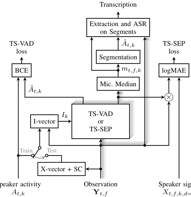
Fig. 2. System overview: Pre training with TS-VAD loss, training with TSSEP loss and predicting transcriptions at inference. Microphones indicated as “shading”.
图 2: 系统概览: 使用TS-VAD损失进行预训练, 使用TSSEP损失进行训练, 并在推理时预测转录文本。麦克风以"阴影"表示。
where $t~\in~{1,\ldots,T}$ and $f\in{1,\ldots,F}$ are the time frame and frequency bin indices, and $T$ and $F$ are the total number of time frames and frequency bins, respectively, while $\mathbf{Y}{t,f}$ , $\mathbf{X}{t,f,k}$ , and $\mathbf{N}{t,f}$ are the STFTs of $\mathbf{y}{\ell}$ , $\mathbf{x}{\ell,k}$ , and $\mathbf{n}{\ell}$ , respectively. Further, $A_{t,k}\in{0,1}$ is the activity of the $k$ -th speaker at frame $t$ , which is derived from $a_{\ell,k}$ by temporally quantizing to time frame resolution.
其中 $t~\in~{1,\ldots,T}$ 和 $f\in{1,\ldots,F}$ 分别表示时间帧和频段的索引,$T$ 和 $F$ 则分别是总时间帧数和总频段数。而 $\mathbf{Y}{t,f}$、$\mathbf{X}{t,f,k}$ 和 $\mathbf{N}{t,f}$ 分别是 $\mathbf{y}{\ell}$、$\mathbf{x}{\ell,k}$ 和 $\mathbf{n}{\ell}$ 的短时傅里叶变换 (STFT)。此外,$A_{t,k}\in{0,1}$ 表示第 $k$ 个说话者在第 $t$ 帧的活动状态,这是通过对 $a_{\ell,k}$ 进行时间帧分辨率量化得到的。
III. TS-VAD
III. TS-VAD
In the CHiME-6 challenge, target-speaker voice activity detection (TS-VAD) [8], [18] achieved impressive results for the di ari z ation task, outperforming other approaches by a large margin. The basic idea is similar to personal VAD [19]: an NN is trained to predict the speech activity $\boldsymbol{A}{t,k}$ of a target speaker $k$ from a mixture $\mathbf{Y}{t,f}$ , given an embedding $I_{k}$ representing the speaker, as illustrated in Fig. 1.
在CHiME-6挑战赛中,目标说话人语音活动检测 (TS-VAD) [8][18] 在语音分离任务中取得了显著成果,大幅领先其他方法。其核心思想与个人语音活动检测 (personal VAD) [19] 类似:如图 1 所示,给定代表说话人的嵌入向量 $I_{k}$,通过神经网络从混合语音 $\mathbf{Y}{t,f}$ 中预测目标说话人 $k$ 的语音活动 $\boldsymbol{A}_{t,k}$。
TS-VAD has two main differences to prior work: first, the speaker embeddings are estimated from the recording instead of utilizing enrollment utterances, as illustrated in Fig. 2, and second, a combination layer estimates the activities of all speakers in a segment simultaneously, given an embedding for each speaker, as illustrated in Fig. 1.
TS-VAD与先前工作有两大主要区别:首先,如图2所示,说话人嵌入(embedding)是从录音中估算得出,而非使用注册语音样本;其次,如图1所示,在给定每个说话人嵌入的情况下,组合层会同时估算片段中所有说话人的活动状态。
A. Speaker embedding estimation
A. 说话人嵌入估计
Here, $\operatorname{Emb}{\cdot}$ symbolizes the computation of the embedding vector from segments of speech from the first microphone where a single speaker is active. Furthermore, $\hat{\boldsymbol{a}}_{\ell,k}$ is an estimate for aℓ,k.
这里,$\operatorname{Emb}{\cdot}$ 表示从第一个麦克风中仅包含单个说话者的语音片段计算嵌入向量。此外,$\hat{\boldsymbol{a}}_{\ell,k}$ 是对 aℓ,k 的估计。
While this approach does not require an enrollment utterance, it makes TS-VAD dependent on another, initial diarization system. Thus, TS-VAD can be viewed as a refinement system: given the estimate of a first di ari z ation, TS-VAD is applied to estimate a better di ari z ation. In [18], it was reported that I-vector embeddings are superior to $\mathrm{X}$ -vectors for TSVAD, which is in contrast to other publications that suggest a superiority of X-vectors over I-vectors for di ari z ation tasks [25]. We follow [18] and use I-vectors.
虽然这种方法不需要注册语音,但它使得 TS-VAD 依赖于另一个初始的说话人日志系统。因此,TS-VAD 可视为一种优化系统:在给定初始说话人日志估计的基础上,应用 TS-VAD 来获得更优的日志结果。[18] 中指出,对于 TS-VAD 任务,I-vector 嵌入优于 $\mathrm{X}$-vector,这与其它文献提出的 X-vector 在说话人日志任务中优于 I-vector 的结论 [25] 相反。我们遵循 [18] 的方法,采用 I-vector。
B. TS-VAD architecture
B. TS-VAD 架构
The TS-VAD network consists of three components, with stacking operations between them, as shown in Fig. 1. First, the logarithmic spec tr ogram and the logarithmic mel filterbank features of one microphone of the mixture are stacked and encoded by a few speaker-independent layers, which can be viewed as feature extraction layers, into matrices with dimension $\mathbb{R}^{T\times Z_{1}}$ , where $Z_{1}$ is the size of a single framewise representation.
TS-VAD网络由三个组件构成,组件间采用堆叠操作连接,如图1所示。首先,混合信号中单个麦克风的对数频谱图和对数梅尔滤波器组特征经过若干说话人无关层的堆叠编码(可视为特征提取层),转换为维度为$\mathbb{R}^{T\times Z_{1}}$的矩阵,其中$Z_{1}$表示单帧表征的尺寸。
Next, for each speaker $k$ , the framewise representation is concatenated with the speaker embedding of that speaker, resulting in an input to the second network component of dimension $\mathbb{R}^{T\times(Z_{1}+E)}$ . This second network component processes each speaker independently, nevertheless the NN layer parameters are shared between the speakers. As a consequence, a discrimination of the speakers can only be achieved through the speaker embeddings, not through the NN layer parameters. For each speaker, the output of the second network component has a dimension of $\mathbb{R}^{T\times Z_{2}}$ , with $Z_{2}$ denoting the size per frame. Until this point, the NN design matches that of personal VAD [19].
接下来,对于每个说话者 $k$,将帧级表示与该说话者的说话者嵌入(embedding)拼接,形成维度为 $\mathbb{R}^{T\times(Z_{1}+E)}$ 的输入,作为第二网络组件的输入。该第二网络组件独立处理每个说话者,但其神经网络层参数在说话者间共享。因此,说话者的区分只能通过说话者嵌入实现,而非神经网络层参数。每个说话者在第二网络组件输出的维度为 $\mathbb{R}^{T\times Z_{2}}$,其中 $Z_{2}$ 表示每帧的大小。至此,神经网络设计与personal VAD [19]保持一致。
Before the last NN layers, the hidden features of all speakers are concatenated to obtain one large feature matrix of dimension $\mathbb{R}^{T\times(K\cdot Z_{2})}$ . The final layers produce an output of dimension $\mathbb{R}^{T\times K}$ , which, after threshold ing and smoothing (see Section IV-C), gives the activity estimate $\hat{A}_{t,k}$ for all speakers $k$ and frames $t$ simultaneously. This combined estimation makes it easier to distinguish between similar speakers. In fact, it was shown in [18] that the combined estimation layers at the end were instrumental in obtaining good performance.
在最后的神经网络层之前,所有说话者的隐藏特征会被拼接成一个维度为$\mathbb{R}^{T\times(K\cdot Z_{2})}$的大型特征矩阵。最终层输出维度为$\mathbb{R}^{T\times K}$的结果,经过阈值化和平滑处理(参见第IV-C节)后,同时得到所有说话者$k$和帧$t$的活动估计$\hat{A}_{t,k}$。这种联合估计方式更易于区分相似说话者。实际上,[18]的研究表明,末端的联合估计层对获得良好性能起到了关键作用。
From this description, it is obvious that TS-VAD assumes knowledge of the total number $K$ of speakers in the meeting to be diarized, because $K$ defines the dimensionality of the network output. This constraint can be relaxed by incorporating an attention mechanism as was shown in [21], for the case of fully overlapped speech separation. Nevertheless, we keep the original TS-VAD stacking, only increasing the number of speakers from 4 in [18] to 8. We do so first because an upper bound of 8 speakers is already large for many meetings, and second to allow for a better comparison with [20], where this stacking is also used.
从这段描述可以明显看出,TS-VAD需要预先知道待分割会议中的说话人总数K,因为K决定了网络输出的维度。虽然文献[21]已证明通过引入注意力机制可以放宽这一限制(针对完全重叠语音分离场景),但我们仍保持原始TS-VAD堆叠结构,仅将说话人数量从文献[18]的4人提升至8人。这样做首先是因为8人上限对多数会议场景已足够大,其次是为了与同样采用该堆叠结构的文献[20]进行更有效的对比。
C. From single-channel to multi-channel
C. 从单通道到多通道
When multiple channels are available, there are different approaches to utilize them, e.g., via spatial features like inter channel phase differences (IPD) [28], for intermediate signal reduction such as in an attention layer [18], and output signal reduction [29]. Each of them has different advantages and disadvantages. We use here an output signal reduction: this means the NN is applied independently to each channel and the output is reduced to a single estimate with a median operation. Incorporating multiple channels in this way allowed us to train the NN with a single channel and use all channels at test time. Besides this, this makes our method agnostic to the array geometry and number of microphones, and the presence of moving speakers, as in CHiME-6 [1], becomes less critical. Finally, this approach was shown to be robust to a mismatch between simulated training data and real test data [29].
当存在多个通道时,可采用不同方法利用它们,例如通过空间特征(如通道间相位差(IPD) [28])、中间信号降维(如在注意力层[18]中)或输出信号降维[29]。每种方法各有优劣。本文采用输出信号降维方案:即神经网络(NN)独立处理每个通道后,通过中值运算将输出降维为单一估计值。这种多通道整合方式使我们能够用单通道数据训练神经网络,而在测试时使用全部通道。此外,该方法对阵列几何结构和麦克风数量具有无关性,且如CHiME-6[1]所示,移动说话人的影响也会降低。最后,该方法被证明能有效应对模拟训练数据与真实测试数据不匹配的情况[29]。
For ease of notation, we ignore microphone indices for the NN input and output in the following section. At training time, we use only a reference microphone, and at test time, the NN is applied independently to each microphone and then the median is used.
为便于表述,下文将忽略神经网络输入和输出中的麦克风索引。训练时仅使用参考麦克风,测试时则独立地将神经网络应用于每个麦克风,随后取中位数。
IV. FROM TS-VAD TO TS-SEP
IV. 从 TS-VAD 到 TS-SEP
We are now going to describe our modifications to the TS-VAD architecture in order to do joint di ari z ation and separation. The key difference between di ari z ation and (maskbased) separation is that di ari z ation output has time resolution, while separation requires time-frequency resolution.
我们现在将描述对TS-VAD架构的修改,以实现联合说话人日志(diarization)和分离。说话人日志与(基于掩码的)分离的关键区别在于,说话人日志输出具有时间分辨率,而分离需要时频分辨率。
A. From Frame to Time-Frequency Resolution
A. 从帧到时频分辨率
Starting from the TS-VAD system, the output size of the last layer is changed from $K$ speakers to $K$ speakers times $F$ frequency bins: $\mathbb{R}^{T\times K}\rightarrow\mathbb{R}^{T^{\setminus}(F\cdot K)}$ , where $\rightarrow$ denotes the “repeat” operation, which is done by repeating the weights of the last layer. Rearranging the output from $\mathbb{R}^{T\times(F\cdot K)}$ to $\mathbb{R}^{T\times F\times K}$ , we obtain a $(T\times F)$ -dimensional spectro-temporal output for each speaker $k$ . With a sigmoid non linearity, which ensures that values are in $[0,1]$ , this can be interpreted as a mask $m_{t,f,k},\forall t,f,k$ , that can be used for source extraction, for example via masking:
从TS-VAD系统出发,将最后一层的输出维度从$K$个说话人改为$K$个说话人乘以$F$个频点:$\mathbb{R}^{T\times K}\rightarrow\mathbb{R}^{T^{\setminus}(F\cdot K)}$,其中$\rightarrow$表示通过重复最后一层权重实现的"复制"操作。将$\mathbb{R}^{T\times(F\cdot K)}$的输出重排为$\mathbb{R}^{T\times F\times K}$后,我们得到每个说话人$k$对应的$(T\times F)$维时频谱输出。通过sigmoid非线性函数(确保数值落在$[0,1]$区间)处理后,可将其解释为掩码$m_{t,f,k},\forall t,f,k$,该掩码可用于语音分离任务,例如通过掩蔽操作实现:
$$
\hat{X}{t,f,k}=m_{t,f,k}Y_{t,f,d=1},
$$
$$
\hat{X}{t,f,k}=m_{t,f,k}Y_{t,f,d=1},
$$
where $d=1$ is the reference microphone. We denote this system as target-speaker separation (TS-SEP).
其中 $d=1$ 为参考麦克风。我们将此系统称为目标说话人分离 (TS-SEP)。
The sketches at the top of Fig. 1 illustrate the different outputs of TS-VAD and TS-SEP and Fig. 2 gives an overview of TS-SEP, whose components are described in the following.
图 1 顶部的示意图展示了 TS-VAD 和 TS-SEP 的不同输出结果,图 2 则概述了 TS-SEP 的结构,其组件将在下文中详细描述。
B. Training Schedule and Objective
B. 训练计划与目标
As TS-SEP emerged from TS-VAD, an obvious choice for training is a two-stage training schedule: in the first, pre training stage, an ordinary TS-VAD system is trained, until it starts to distinguish between speakers; then, the last layer is copied $F$ times to obtain the desired time-frequency resolution; the second training stage is then the training of the
由于 TS-SEP 源自 TS-VAD,一个明显的训练选择是采用两阶段训练方案:在第一预训练阶段,先训练一个普通的 TS-VAD 系统,直到它能够区分说话人;接着将最后一层复制 $F$ 次以获得所需的时频分辨率;随后第二训练阶段即对
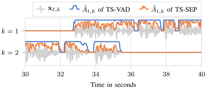
Fig. 3. Estimated speaker activity $\tilde{A}{}{t,k}$ for 2 of 8 speakers from the LibriCSS DEV OV40 dataset, shown together with the corresponding clean speaker time signals $\mathbf{x}_{\ell,k}$ . Best viewed in color.
图 3: LibriCSS DEV OV40 数据集中 8 个说话人里 2 个的估计说话人活动度 $\tilde{A}{}{t,k}$,与对应的纯净说话人时间信号 $\mathbf{x}_{\ell,k}$ 一同展示。建议彩色查看。
TS-SEP system, initialized with the parameters of the TS-VAD system.
TS-SEP系统,使用TS-VAD系统的参数进行初始化。
For the TS-VAD pre training, we used the training loss proposed in the original publication [18], which is the sum of the binary cross entropy (BCE) losses between estimated and ground-truth activities for all speakers.
对于TS-VAD的预训练,我们采用了原始文献[18]提出的训练损失函数,即所有说话人估计活动与真实活动之间的二元交叉熵(BCE)损失之和。
There are several choices for the training objective of the TS-SEP system. We opted for a time-domain reconstruction loss, since it implicitly accounts for phase information (see [30], [31] for a discussion of time- vs. frequency-domain reconstruction losses). To be specific, a time-domain signal reconstruction loss is computed by applying an inverse STFT to $\hat{X}{t,f,k}$ to obtain $\hat{x}{\ell,k}$ and measuring the logarithmic mean absolute error (LogMAE) from the ground truth $x_{\ell,k}$ :
TS-SEP系统的训练目标有几种选择。我们选择了时域重建损失,因为它隐含地考虑了相位信息(关于时域与频域重建损失的讨论参见[30]、[31])。具体而言,通过对$\hat{X}{t,f,k}$应用逆短时傅里叶变换得到$\hat{x}{\ell,k}$,并计算其与真实值$x_{\ell,k}$的对数平均绝对误差(LogMAE)来获得时域信号重建损失:
$$
\mathcal{L}=\log_{10}\frac{1}{L}\sum_{k}\sum_{\ell}\left|\hat{x}{\ell,k}-x_{\ell,k}\right|.
$$
$$
\mathcal{L}=\log_{10}\frac{1}{L}\sum_{k}\sum_{\ell}\left|\hat{x}{\ell,k}-x_{\ell,k}\right|.
$$
Clearly, other loss functions, such as the MAE, mean squared error (MSE), or signal-to-distortion ratio (SDR) can also be employed. However, it is important to note that for reconstruction losses that contain a log operation, the sum across the speakers should be performed before applying the log operation. Otherwise, the loss is undefined and the training can become unstable if a speaker is completely silent [32].
显然,也可以使用其他损失函数,如 MAE (平均绝对误差)、MSE (均方误差) 或 SDR (信噪比)。但需要注意的是,对于包含对数运算的重构损失,应在应用对数运算之前对各扬声器进行求和。否则,如果扬声器完全静音,损失将无法定义且训练可能变得不稳定 [32]。
We also experimented with training the TS-SEP system from scratch. However, this turned out to be far more sensitive to the choice of training loss. We found that only a modified binary cross entropy loss, where we artificially gave a higher weight to loss contributions corresponding to “target present”, was able to learn from scratch, while other choices did not converge at all1. But even with this loss, the final performance was worse than with the two-stage training2. Here, we therefore only report experiments with the described two-stage training.
我们还尝试了从头开始训练 TS-SEP 系统。然而,这种方法对训练损失函数的选择极为敏感。我们发现,只有采用改进的二元交叉熵损失(人为赋予"目标存在"情况更高权重)时才能实现从零学习,而其他损失函数选择完全无法收敛[1]。但即便使用该损失函数,最终性能仍不及两阶段训练方案[2]。因此,本文仅汇报所述两阶段训练的实验结果。
C. Activity estimation / Segmentation
C. 活动估计/分割
TS-SEP outputs a mask with TF resolution. To get an estimate like TS-VAD with only time resolution, we take the
TS-SEP输出一个具有时频(TF)分辨率的掩码。为了获得像TS-VAD那样仅具有时间分辨率的估计值,我们采用
1The networks learned first to predict only zeros and were not able to leave these local optima.
1这些网络最初只学会了预测零值,无法跳出这些局部最优解。
$^2\mathrm{In}$ some preliminary experiments, we obtained $8.72%$ concatenated minimum-permutation word error rate (cpWER) for two-stage training, while training from scratch led to $100%$ cpWER with the LogMAE loss (because of zero estimates) and $12.0%$ cpWER with the binary cross entropy-based loss.
$^2\mathrm{在}$ 一些初步实验中,我们通过两阶段训练获得了 $8.72%$ 的拼接最小排列词错误率 (cpWER) ,而从头开始训练时,使用 LogMAE 损失函数 (由于零估计) 导致 $100%$ 的 cpWER,使用基于二元交叉熵的损失函数则得到 $12.0%$ 的 cpWER。
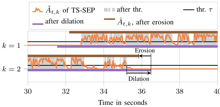
Fig. 4. Threshold ing and “closing” morphological operation (dilation followed by erosion) on $\tilde{A}{t,k}^{\mathrm{~~}}$ to obtain $\hat{A}_{t,k}$ , for 2 of 8 speakers from the LibriCSS DEV OV40 dataset. Best viewed in color.
图 4: 对 $\tilde{A}{t,k}^{\mathrm{~~}}$ 进行阈值化和"闭运算"形态学操作(先膨胀后腐蚀)以得到 $\hat{A}_{t,k}$ ,展示了LibriCSS DEV OV40数据集中8个说话人中的2个示例。建议彩色查看。
mean across the frequencies:
频率均值:
$$
\tilde{A}{t,k}=\frac{1}{F}\sum_{f}m_{t,f,k}.
$$
$$
\tilde{A}{t,k}=\frac{1}{F}\sum_{f}m_{t,f,k}.
$$
Typically, this estimate has spikes for each word and is close to zero between words, see Fig. 3. To fill those gaps, we followed [6] and used threshold ing and the “closing” morphological operation (see Fig. 4), known from image processing [33]: in a first dilation step, a sliding window is moved over the signal with a shift of one, and the maximum value inside the window is taken as the new value for its center sample; in a subsequent erosion step, we do the same, however with the minimum operation, leading to the final smoothed activity estimate
通常,这个估计值在每个单词处会出现峰值,在单词之间则接近于零,见图 3。为了填补这些间隙,我们参考 [6] 采用了阈值处理和来自图像处理 [33] 的“闭运算”形态学操作(见图 4):在第一步膨胀操作中,滑动窗口以步长 1 在信号上移动,并将窗口内的最大值作为中心样本的新值;在随后的腐蚀操作中,我们采用相同方式但使用最小值运算,最终得到平滑后的活动估计。
$$
\hat{A}{t,k}=\operatorname{Erosion}(\operatorname{Dilation}(\delta(\tilde{A}_{t,k}\geq\tau))).
$$
$$
\hat{A}{t,k}=\operatorname{Erosion}(\operatorname{Dilation}(\delta(\tilde{A}_{t,k}\geq\tau))).
$$
Here, $\tau$ is the threshold and $\delta(x)$ denotes the Kronecker delta which evaluates to one if $x$ is true and zero otherwise. When the window for the dilation is larger than the window for erosion, the speech activity is overestimated, i.e., the difference divided by two is added to the beginning and end of the segment, as illustrated in Fig. 4. While an over estimation will likely worsen the di ari z ation performance, this may not be the case for automatic speech recognition (ASR): it is indeed common to train ASR systems with recordings that contain a single utterance plus some silence (or background noise) at the beginning and end of the recording. We investigate the over estimation later in Section V-H.
这里,$\tau$ 是阈值,$\delta(x)$ 表示克罗内克函数 (Kronecker delta),当 $x$ 为真时其值为1,否则为0。当膨胀操作的窗口大于腐蚀操作的窗口时,语音活动会被高估,即差值的一半会被添加到片段的开始和结束处,如图 4 所示。虽然高估可能会降低语音活动检测性能,但对于自动语音识别 (ASR) 来说可能并非如此:实际上,训练 ASR 系统时通常会使用包含单个语音片段并在录音开头和结尾带有一些静音(或背景噪声)的录音。我们将在第 V-H 节中进一步研究高估问题。
At activity change points of $\hat{A}_{t,k}$ , the speakers’ signals are cut, leading to segments of constant speaker activity.
在 $\hat{A}_{t,k}$ 的活动变化点处,说话者的信号被切断,导致产生恒定说话者活动的片段。
This threshold ing and “closing” procedure departs from the median-based smoothing typically used for TS-VAD. When the di ari z ation system is trained to fill gaps of short inactivity (e.g., pauses between words), median-based smoothing is fine. But in TS-SEP, the system is trained to predict a timefrequency reconstruction mask for each speaker, so typically the mask values are smaller than the VAD values, short inactivity produces zeros, and values are smaller in overlap regions than in non-overlap regions. The threshold ing and closing morphological operations help to fill the gaps.
该阈值处理和"闭合"操作不同于TS-VAD常用的基于中值的平滑方法。当二值化系统被训练用于填补短暂静默间隙(如词语间的停顿)时,基于中值的平滑方法效果良好。但在TS-SEP中,系统被训练为每个说话者预测时频重建掩码,因此掩码值通常小于语音活动检测(VAD)值,短暂静默会产生零值,且重叠区域的数值小于非重叠区域。阈值处理和形态学闭合操作有助于填补这些间隙。
D. Extraction
D. 提取
At evaluation time, an estimate of the signal of speaker $k$ is obtained by multiplying the mask with the STFT of the input speech, see Eq. (5). If multi-channel input is available, an alternative to mask multiplication for source extraction is to utilize the estimated masks to compute beamformer coefficients [29]. For beam forming, the spatial covariance matrices of the desired signal
在评估阶段,通过将掩码与输入语音的短时傅里叶变换 (STFT) 相乘来估计说话人 $k$ 的信号,参见式 (5)。若存在多通道输入,另一种源信号提取方法是通过估计的掩码计算波束成形系数 [29]。对于波束成形,需计算目标信号的空间协方差矩阵
$$
\Phi_{x x,f,b}=\frac{1}{\left|{\cal T}{b}\right|}\sum_{t\in\mathcal{T}{b}}m_{t,f,k_{b}}{\bf Y}{t,f}{\bf Y}_{t,f}^{\mathrm{H}}
$$
$$
\Phi_{x x,f,b}=\frac{1}{\left|{\cal T}{b}\right|}\sum_{t\in\mathcal{T}{b}}m_{t,f,k_{b}}{\bf Y}{t,f}{\bf Y}_{t,f}^{\mathrm{H}}
$$
and of the distortion
失真
$$
\Phi_{d d,f,b}=\frac{1}{|\mathcal{T}{b}|}\sum_{t\in\mathcal{T}{b}}\operatorname*{max}\left(\varepsilon,\sum_{\tilde{k}\neq k_{b}}m_{t,f,\tilde{k}}\right)\mathbf{Y}{t,f}\mathbf{Y}_{t,f}^{\mathrm{H}}
$$
$$
\Phi_{d d,f,b}=\frac{1}{|\mathcal{T}{b}|}\sum_{t\in\mathcal{T}{b}}\operatorname*{max}\left(\varepsilon,\sum_{\tilde{k}\neq k_{b}}m_{t,f,\tilde{k}}\right)\mathbf{Y}{t,f}\mathbf{Y}_{t,f}^{\mathrm{H}}
$$
are first computed. Here, $b$ denotes the segment index, $\tau_{b}$ is the set of frame indices that belong to segment $b$ , $k_{b}$ is the index of the speaker active in segment $b$ who is to be extracted3, $\varepsilon=$ 0.0001 is a small value introduced for stability, and kk denotes the summation over all speaker indices, exce pt $k_{b}$ .
首先进行计算。这里,$b$ 表示段索引,$\tau_{b}$ 是属于段 $b$ 的帧索引集合,$k_{b}$ 是段 $b$ 中待提取的活跃说话人索引3,$\varepsilon=$ 0.0001 是为稳定性引入的小值,kk 表示对所有说话人索引(除 $k_{b}$ 外)的求和。
With these covariance matrices, the beamformer coefficients can be computed for example using a minimum variance distort ion less response (MVDR) beamformer in the formulation of [34]:
利用这些协方差矩阵,可以计算波束形成系数,例如采用[34]中提出的最小方差无失真响应(MVDR)波束形成器:
$$
\begin{array}{r}{\mathbf{w}{f,b}=\mathrm{MVDR}(\Phi_{x x,f,b},\Phi_{d d,f,b}).}\end{array}
$$
$$
\begin{array}{r}{\mathbf{w}{f,b}=\mathrm{MVDR}(\Phi_{x x,f,b},\Phi_{d d,f,b}).}\end{array}
$$
Finally, source extraction is performed by applying the beamformer to the input speech:
最后,通过将波束形成器应用于输入语音来执行源提取:
$$
\hat{X}{t,f,k_{b}}=\mathbf{w}{f,b}^{\mathrm{H}}\mathbf{Y}{t,f},\quad\forall t\in\mathcal{T}_{b}.
$$
$$
\hat{X}{t,f,k_{b}}=\mathbf{w}{f,b}^{\mathrm{H}}\mathbf{Y}{t,f},\quad\forall t\in\mathcal{T}_{b}.
$$
In our experiments, we also combined beam forming with mask multiplication [35], which led to somewhat better suppression of competing speakers:
在我们的实验中,我们还结合了波束成形(beam forming)与掩码乘法(mask multiplication) [35],这在一定程度上更好地抑制了竞争说话者:
$$
\hat{X}{t,f,k_{b}}=\mathbf{w}{f,b}^{\mathrm{H}}\mathbf{Y}{t,f}\operatorname*{max}(m_{t,f,k_{b}},\xi),\quad\forall t\in\mathcal{T}_{b},
$$
$$
\hat{X}{t,f,k_{b}}=\mathbf{w}{f,b}^{\mathrm{H}}\mathbf{Y}{t,f}\operatorname*{max}(m_{t,f,k_{b}},\xi),\quad\forall t\in\mathcal{T}_{b},
$$
where $\xi\in[0,1]$ is a lower bound/threshold for the mask.
其中 $\xi\in[0,1]$ 是掩码的下界/阈值。
The lower bound can be motivated by the observations from [36]: pure NN based speech enhancement can degrade the ASR performance compared to doing nothing; when adding a scaled version of the observation to the enhanced signal, the ASR performance can improve compared to doing nothing.
下界可以通过[36]中的观察结果得到解释:与不进行任何处理相比,基于纯神经网络(NN)的语音增强可能会降低自动语音识别(ASR)性能;当向增强信号中添加观测信号的缩放版本时,ASR性能相比不处理会有所提升。
E. Guided Source Separation (GSS)
E. 引导式源分离 (GSS)
An alternative to the immediate use of the mask for extraction is to fine-tune the mask first. If multi-channel input is available, this can be achieved by an SMM, which utilizes spatial information. Here, we employ the GSS proposed in [7], where the guiding information is given by the di ari z ation information $\check{\boldsymbol{A}}{t,k}$ : the posterior probability that the $k$ -th mixture component is active in a frame $t$ can only be non-zero if $\hat{A}{t,k}$ is one. The SMM is applied to segments $b$ whose boundaries are determined by $\hat{A}_{t,k}$ , plus some context. The EM iterations using the guiding information are complemented with a non-guided EM step. The finally estimated class posterior probabilities form the speaker-specific time-frequency masks that are used for source extraction by beam forming. For details on GSS, see [7].
一种替代直接使用掩码进行提取的方法是对掩码先进行微调。如果有多通道输入可用,这可以通过利用空间信息的SMM(空间混合模型)实现。此处我们采用[7]中提出的GSS(引导源分离)方法,其引导信息由二值化信息$\check{\boldsymbol{A}}{t,k}$提供:当$\hat{A}{t,k}$为1时,第$k$个混合成分在帧$t$中活跃的后验概率才可能非零。SMM应用于由$\hat{A}_{t,k}$及其上下文确定的片段$b$。使用引导信息的EM(期望最大化)迭代会辅以一个非引导的EM步骤。最终估计的类别后验概率形成说话人特定的时频掩码,用于通过波束成形进行源提取。关于GSS的详细信息,请参阅[7]。
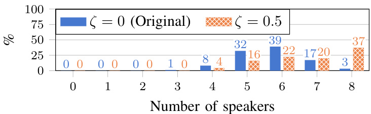
Fig. 5. Distribution of the number of speakers active in 1-minute chunks of the training data, depending on the probability $\zeta$ to use superposition/mixup $\zeta=0$ corresponds to the original dataset without superposition).
图 5: 训练数据中1分钟片段内活跃说话者数量的分布情况,取决于使用叠加/混合 (superposition/mixup) 的概率 $\zeta$ ( $\zeta=0$ 对应未使用叠加的原始数据集)。
While earlier works initialized the SMM by broadcasting voice activity detection (VAD) information $\hat{A}{t,k}^{\mathrm{~~}}$ over the frequency axis that was available either from manual annotation (CHiME-5 [37]) or determined automatically (CHiME-6 Track 2 [1]), we here propose to initialize the posterior of the SMM with $m_{t,f,k}$ , which is only available for TS-SEP, while voice activity information $\hat{A}_{t,k}$ is available for TS-VAD and TS-SEP.
早期研究通过沿频率轴广播语音活动检测 (VAD) 信息 $\hat{A}{t,k}^{\mathrm{~~}}$ 来初始化 SMM (speaker mask model),这些信息或来自人工标注 (CHiME-5 [37]) 或通过自动检测确定 (CHiME-6 Track 2 [1])。本文提出使用 $m_{t,f,k}$ 初始化 SMM 后验概率,该参数仅适用于 TS-SEP (target speaker separation),而语音活动信息 $\hat{A}_{t,k}$ 则同时适用于 TS-VAD (target speaker voice activity detection) 和 TS-SEP。
V. EXPERIMENTS
五、实验
A. Training and Test Datasets
A. 训练与测试数据集
Di ari z ation and recognition experiments are carried out on the LibriCSS data set, which is a widely used data set for evaluating meeting recognition systems [3]. It contains rerecordings of loudspeaker playback of Libri Speech sentences mixed in a way to reflect a typical meeting scenario. The dataset consists of 10 one-hour-long sessions, where each session is subdivided into six 10-minute-long mini sessions that have different overlap ratios, ranging from 0 to $40%$ . In each session, a total of eight speakers are active. The recording device was a seven-channel circular microphone array. Following [2], we used the first session as development (DEV) set and the other 9 as evaluation (EVAL) set.
在LibriCSS数据集上进行了切分和识别实验,该数据集是广泛用于评估会议识别系统的基准[3]。它包含通过扬声器重放的LibriSpeech句子混合录音,模拟典型会议场景。数据集包含10个时长1小时的会话,每个会话被细分为6段10分钟的片段,各片段具有0%至40%的不同重叠比例。每个会话共有8名活跃说话人,录音设备采用七通道环形麦克风阵列。参照[2]的方法,我们使用第一个会话作为开发(DEV)集,其余9个作为评估(EVAL)集。
As training data, we employed simulated meeting data created with scripts4 from the LibriCSS authors. While each training meeting contains 8 speakers, we trained only on chunks of 1 minute. Since within a chunk usually fewer speakers are active, as shown in Fig. 5, we superposed segments of speech to artificially increase the number of active speakers, see Section V-D for a discussion on this.
作为训练数据,我们采用了LibriCSS作者用脚本生成的模拟会议数据。虽然每次训练会议包含8位发言者,但我们仅对1分钟的片段进行训练。如图5所示,由于单个片段内通常活跃发言者较少,我们通过叠加语音片段人为增加了活跃发言者数量(具体讨论见第V-D节)。
B. Performance Measures
B. 性能指标
Since this work focuses on meeting transcription enriched with information about who spoke when, we measure both di ari z ation and word error rate performance.
由于本研究重点关注包含说话人时间信息的会议转录,因此我们同时测量了说话人分离 (diarization) 和词错误率 (word error rate) 性能。
As the di ari z ation performance measure, we employ the widely used di ari z ation error rate (DER), which is measured with the “md-eval-22.pl” script from NIST [38]. The DER is the sum of false alarms, missed hits, and speaker confusion errors divided by the total speaker time.
作为日记化性能衡量指标,我们采用广泛使用的日记化错误率(DER),该指标通过NIST的"md-eval-22.pl"脚本[38]进行测量。DER是误报、漏报和说话人混淆错误的总和除以总说话时长。
For the recognition of partially overlapping speech of multiple speakers, there are several word error rate (WER) definitions [39]. Since TS-VAD groups utterances of the same speaker, we mainly report the concatenated minimumpermutation word error rate (cpWER), where all transcriptions of one speaker are concatenated and the word error rate is computed on the mapping between estimated transcriptions and the ground-truth word sequences of the different speakers that results in the lowest word error rate.
针对多人部分重叠语音的识别,存在多种词错误率 (WER) 定义 [39]。由于 TS-VAD 会对同一说话人的语音片段进行分组,我们主要报告拼接最小排列词错误率 (cpWER) —— 该方法将所有同一说话人的文本转录拼接起来,通过计算估计转录与不同说话人真实词序列之间的映射关系(选择能产生最低词错误率的映射方案)来得出最终词错误率。
Note that the cpWER also counts recognition errors caused by wrong di ari z ation. For example, if the di ari z ation swaps the speaker identity of an utterance, this adds to the deletion error count of the correct speaker’s transcription, and, furthermore, adds to the insertion error count of the wrongly identified speaker, regardless of whether the recognized words were correct or not.
需要注意的是,cpWER (concatenated minimum-permutation word error rate) 也会统计因错误说话人分离 (diarization) 导致的识别错误。例如,若说话人分离环节交换了某段语音的说话人身份,无论识别文本是否正确,这都会计入正确说话人转录文本的删除错误数,同时会计入错误识别说话人的插入错误数。
Since we are interested in knowing the contribution of di ari z ation errors, we also computed the assignment $k_{b}$ of recognized segment transcriptions to the ground-truth transcription streams such that the cpWER is as small as possible. In other words, we use as the speaker label for each segment $b$ the label that minimizes the cpWER, instead of the estimated speaker label $k_{b}$ that was obtained from $\hat{A}_{t,k}$ , while keeping the estimated segment start and end times. This is similar to the MIMO-WER defined in [39], but ground-truth and estimate are swapped. The error rate computed in this way ignores contributions from di ari z ation errors, hence we call it di ari z ation invariant concatenated minimum-permutation word error rate (DI-cpWER). The difference between the cpWER and DI-cpWER can then be interpreted as the errors caused by di ari z ation mistakes.
由于我们关注的是说话人日志 (diarization) 错误的贡献度,因此还计算了识别片段转写结果到真实转写流的最优分配 $k_{b}$ ,使得 cpWER 尽可能小。换句话说,对于每个片段 $b$ ,我们使用使 cpWER 最小化的标签作为说话人标签,而非从 $\hat{A}{t,k}$ 获得的估计说话人标签 $k{b}$ ,同时保留估计的片段起止时间。这与 [39] 中定义的 MIMO-WER 类似,但互换了真实值和估计值的位置。通过这种方式计算的错误率忽略了说话人日志错误的贡献,因此我们称之为说话人日志不变的拼接最小置换词错误率 (DI-cpWER)。cpWER 与 DI-cpWER 之间的差值可解释为说话人日志错误导致的误差。
In the literature, the asclite tool is often used to compute the WER of multi-speaker transcriptions [40]. It ignores diarization errors as well, but is limited to shorter segments and fewer estimated “speakers”. It has been used on LibriCSS in the past, however with so-called continuous speech separation (CSS) systems that separate the data into two streams where each stream contains the signals of several speakers who do not overlap [3]. In our setup, we produce eight streams, one for each speaker in the meeting, and because the computation and memory demands of asclite increase exponentially with the number of streams, it is computationally infeasible to use asclite for our system.
文献中常用asclite工具计算多说话人转写的词错误率(WER) [40]。该工具同样忽略说话人日志错误,但仅适用于较短片段和较少预估"说话人"的场景。过去它曾被用于LibriCSS数据集,但仅限于所谓的连续语音分离(CSS)系统——这类系统将数据分离为两条流,每条流包含若干互不重叠说话人的信号[3]。在我们的配置中,系统会生成八条流(对应会议中每位说话人),由于asclite的计算量和内存需求随流数量呈指数级增长,对我们的系统而言使用该工具在计算上不可行。
Both asclite and DI-cpWER calculate a WER where diarization errors are ignored. The numbers obtained are thus roughly comparable, and we shall use speaker agnostic WER (WER) as a general name for those WERs that ignore di ari z ation errors.
asclite和DI-cpWER计算的WER均忽略说话人分离错误。因此所得数值大致可比,我们将使用说话人无关WER (WER)作为这类忽略分离错误的WER统称。
We used two different pretrained ASR systems from the ESPnet framework [41] to estimate the transcription. Both are used “out of the box” without any fine-tuning. The first, which we refer to as “base”5 [42], has a transformer architecture. It is designed and trained on Libri Speech and achieves a WER of $2.7%$ on the clean test set of Libri Speech. The second, which we refer to as “WavLM”6 [43], is a conformer based ASR system that utilizes WavLM [44] features. It is designed for CHiME-4 [45] and uses Libri-Light [46], GigaSpeech [47], VoxPopuli [48], CHiME-4 [45], and WSJ0/1 [49] for training. On the clean test set of Libri Speech, it achieves a WER of $1.9%$ .
我们使用ESPnet框架[41]中的两种不同预训练ASR(自动语音识别)系统来估算转录结果。两者均直接使用"开箱即用"模式,未进行任何微调。第一个系统(我们称为"base"[42])采用Transformer架构,基于Libri Speech数据集设计训练,在Libri Speech干净测试集上达到2.7%的词错误率(WER)。第二个系统(称为"WavLM"[43])是基于Conformer架构的ASR系统,采用WavLM[44]特征,专为CHiME-4[45]设计,训练数据包括Libri-Light[46]、GigaSpeech[47]、VoxPopuli[48]、CHiME-4[45]和WSJ0/1[49],在Libri Speech干净测试集上取得1.9%的词错误率。
The results in the following tables have been obtained using all seven channels of the LibriCSS dataset, unless otherwise stated. Note that masks are estimated for each channel independently, and the median is then applied across the channels to obtain the final mask, see Fig. 2.
以下表格中的结果均使用了LibriCSS数据集的所有七个通道,除非另有说明。请注意,每个通道的掩码是独立估计的,然后对各通道应用中位数以得到最终掩码,见图2。
C. Preprocessing
C. 预处理
The speech data is transformed to the STFT domain with a $64\mathrm{ms}$ window and 16 ms shift. In the STFT domain, the logarithmic spec tr ogram and mel frequency cepstral coefficients (MFCC) are stacked as input features for the NN.
语音数据通过64ms窗口和16ms移位的STFT变换到频域。在STFT域中,对数频谱图(logarithmic spectrogram)和梅尔频率倒谱系数(MFCC)被堆叠作为神经网络的输入特征。
For the computation of the speaker embeddings, we followed [18]: at training time, we used oracle annotations to identify single-speaker regions, from which I-vectors are estimated; at test time, we employed an X-vector extractor and spectral clustering (SC) from the ESPnet LibriCSS recipe [41] to obtain estimates of the annotations, to be used for I-vector extraction 7. Note that this initial estimate is unable to identify overlapping speech, and thus overlapping speech cannot be excluded for the embedding calculation.
在说话人嵌入的计算上,我们遵循[18]的方法:训练阶段使用标注真值识别单说话人区域并提取I-vector;测试阶段采用ESPnet LibriCSS方案[41]中的X-vector提取器和谱聚类(SC)算法估计标注信息,进而用于I-vector提取7。需注意的是,该初始估计无法识别重叠语音,因此嵌入计算时无法排除重叠语音段。
In Kaldi [50], and hence also in the original implementation of TS-VAD [18], it is common to compute a mean and variance vector for each data set and normalize the input feature vectors with them. We initially skipped this normalization, but we observed a serious performance degradation without this domain adaptation, with an increase of the WER from $7.7%$ to $21.5%$ . Therefore, for all experiments reported here, we employed moment (mean and variance) matching between the simulated validation dataset and the rerecorded DEV and EVAL LibriCSS datasets for the input features and the Ivectors.
在Kaldi [50]以及TS-VAD [18]的原始实现中,通常会对每个数据集计算均值向量和方差向量,并用它们对输入特征向量进行归一化。我们最初跳过了这一归一化步骤,但发现缺乏这种域适应会导致性能严重下降,WER从$7.7%$上升至$21.5%$。因此,在本文报告的所有实验中,我们对模拟验证数据集与重新录制的DEV和EVAL LibriCSS数据集之间的输入特征及Ivectors进行了矩(均值和方差)匹配。
As an additional enhancement, weighted prediction error (WPE) based de reverberation [51], [52] was carried out prior to the NN and the extraction at test time.
作为额外增强措施,在神经网络(NN)和测试阶段特征提取之前,先进行了基于加权预测误差(WPE)的去混响处理 [51][52]。
D. Training Details
D. 训练细节
While developing this system, we found several aspects that had a higher impact on the convergence properties or the final performance than we expected, for example reducing the time until the network starts to learn from weeks to hours. We will not provide detailed experiments for each of the modifications we found useful, but we want to present our findings for the benefit of the community.
在开发该系统时,我们发现某些因素对收敛特性或最终性能的影响超出了预期,例如将网络开始学习的时间从数周缩短至数小时。虽然不会对我们认为有效的每项修改进行详细实验,但希望分享这些发现以回馈社区。
We used one-minute-long chunks of data for the training. To reduce the dependency on the artificial speaker ordering, we followed [18] in randomly permuting the speaker embeddings at the input and reversing the permutation after the NN.
我们使用一分钟长的数据块进行训练。为了减少对人工说话人排序的依赖性,我们遵循[18]的方法,在输入时随机排列说话人嵌入,并在神经网络(NN)后反转排列。
TABLE I COMPARISON OF OUR TS-VAD IMPLEMENTATION WITH THAT OF [20], USING VARIOUS DI ARI Z ATION INFORMATION TO SEGMENT THE OBSERVATION AND APPLYING VARIOUS ASR SYSTEMS, WITHOUT INTERMEDIATE SEPARATION OF OVERLAPPING SPEECH. THE FIRST MICROPHONE OF LIBRICSS IS USED.
表 1: 我们的TS-VAD实现与[20]的对比,使用不同语音分割信息对观测进行分段并应用不同ASR系统,不进行重叠语音的中间分离。使用LIBRICSS的第一个麦克风。
| ID | Ref. | Diarization | ASR | DEV DER | EVAL DER | DEV cpWER | EVAL cpWER |
|---|---|---|---|---|---|---|---|
| (1) | [20] Oracle | HMM-DNN | 一 | 23.1 | |||
| (2) | [20] | TS-VAD | HMM-DNN | 一 | 7.6 | 25.8 | |
| (3) | [44] | Oracle | WavLM | 一 | 一 | 6.0 | |
| (4) | Oracle | Base | 0.0 | 0.0 | 19.17 | 19.77 | |
| (5) | SC | Base | 18.93 | 17.93 | 29.07 | 27.77 | |
| (6) | TS-VAD | Base | 6.30 | 5.65 | 21.55 | 21.27 | |
| (7) | TS-VAD | WavLM | 6.30 | 5.65 | 10.39 | 9.13 | |
| (8) | Oracle | WavLM | 0.0 | 0.0 | 6.79 | 6.01 |
Furthermore, we observed a better training convergence when executing the NN two times with different permutations and averaging the outputs, after inverting the permutations, before the last non linearity. This idea was mentioned in [18] to be used for the evaluation of some preliminary experiments.
此外,我们观察到,在执行神经网络两次不同排列并反转排列后、在最终非线性层之前对输出取平均时,训练收敛性更好。这一思路在[18]中被提及用于某些初步实验的评估。
For separation systems, we observed better convergence properties when more overlap was present in the beginning of the training. We also observed this behavior for TSVAD based di ari z ation, hence we used the superposition idea from [53], which is similar to mixup [54] and took, with $\zeta~=~50%$ probability, the sum of a minute of data with the following minute as training data instead of the original data. To compute the TS-VAD targets for this superposition, we used the logical or operator. Although this superposition introduced a mismatch between training and test (e.g., self overlap and more simultaneous and total active speakers), we observed better convergence and a better final performance. We show the distribution of the number of active speakers in the training data with and without superposition in Fig. 5.
对于分离系统,我们观察到在训练初期存在更多重叠时能获得更好的收敛特性。基于TSVAD的说话人日志任务中也发现了这一现象,因此我们采用了[53]提出的叠加思想(类似于mixup[54]),以$\zeta~=~50%$的概率将一分钟数据与下一分钟数据求和作为训练数据,而非使用原始数据。计算这种叠加的TS-VAD目标时,我们采用了逻辑或运算。虽然这种叠加会导致训练与测试之间存在不匹配(例如自重叠、更多同时活跃说话人及总活跃说话人数量增加),但我们观察到了更好的收敛性和最终性能。图5展示了使用与不使用叠加时训练数据中活跃说话人数量的分布对比。
E. Post processing / Segmentation
E. 后处理/分割
For the pretrained ASR system named “base”, we observed a strange behavior for long segments8, hence we split long activities at silence positions, according to $\tilde{A}{}_{t,k}$ , such that no segment is longer than 12 s. As minimum segment length, we used 40 frames (0.64 s), but this was only necessary when no over estimation was used.
对于名为"base"的预训练ASR系统,我们观察到长片段8的异常行为,因此根据$\tilde{A}{}_{t,k}$在静音位置分割长活动片段,确保每个片段不超过12秒。最小片段长度设为40帧(0.64秒),但该设置仅在不使用过估计时必要。
F. Baselines and reference results
F. 基线方法和参考结果
The public source code of TS-VAD [18] is written in Kaldi for the CHiME-6 data, and the modifications for LibriCSS [20] are not publicly available. We re implemented TS-VAD in PyTorch [55] and tried to follow the original implementation as closely as possible. For example, for the NN layers, we used one BLSTMP9 [57], two BLSTMP, and one BLSTMP followed by a feed forward layer for the three NN blocks in
TS-VAD [18] 的公开源代码是用 Kaldi 为 CHiME-6 数据编写的,而针对 LibriCSS [20] 的修改并未公开。我们用 PyTorch [55] 重新实现了 TS-VAD,并尽可能贴近原始实现。例如,在神经网络层方面,我们为三个神经网络模块分别使用了一个 BLSTMP9 [57]、两个 BLSTMP 以及一个带前馈层的 BLSTMP。
TABLE II RESULTS OF TS-SEP WITH VARIOUS ENHANCEMENT STRATEGIES, USING SEGMENTATION HYPER PARAMETERS THR. $\tau=0.6$ , DIL. $=161$ , AND $\mathrm{ERO.}=81\$ .
表 II TS-SEP 采用不同增强策略的结果,使用分割超参数 THR. $\tau=0.6$、DIL. $=161$ 和 $ERO=81$。
| ID | 提取 | DER | cpWER |
|---|---|---|---|
| WPE BF | Masking () | DEV | |
| (1) | 一 | 15.47 | |
| (2) | 15.35 | ||
| (3) | /(0.0) | 15.35 | |
| (4) | /(0.5) | 15.35 | |
| (5) | 一 | 15.35 | |
| (6) | √ /(0.0) | 15.35 | |
| (7) | √ /(0.01) | 15.35 | |
| (8) | /(0.05) | 15.35 | |
| (9) | < /(0.2) | 15.35 | |
| (10) | /(0.5) | 15.35 | |
| (11) | 一 | /(0.5) | 15.47 |
Fig. 1. Nevertheless, they may differ in some details. We therefore first verify if our implementation is competitive. In Table I, we see that the DER and WER of our implementation is similar to the original implementation (lines (6) vs. (2)). The TS-VAD is able to improve over SC (lines (6) vs. (5)) and, with the WavLM-based ASR system, we achieved our best WER without doing any enhancement (line (7)).
图 1: 尽管如此,它们在细节上可能存在差异。因此我们首先验证了自身实现的竞争力。在表 I 中可见,本实现的 DER 和 WER 指标与原版实现相当 (对比行 (6) 与行 (2) )。TS-VAD 能够超越 SC 的表现 (对比行 (6) 与行 (5)),且基于 WavLM 的 ASR 系统在不进行任何增强的情况下实现了最佳 WER 成绩 (行 (7))。
G. Extraction and enhancement
G. 提取与增强
TABLE III RESULTS OF TS-SEP WITH VARIOUS SEGMENTATION HYPER PARAMETERS, USING WPE $\mathrm{i+BF+}$ MASKING $\xi=0.5$ ) ASENHANCEMENT.
表 III 采用 WPE $\mathrm{i+BF+}$ 掩蔽 $\xi=0.5$ ) 作为增强时,TS-SEP 在不同分割超参数下的结果
| ID | 分割 | DER | cpWER | |||
|---|---|---|---|---|---|---|
| Thr. T | Dil. Ero. | DEV | EVAL | DEV | EVAL | |
| (1) | 0.3 201 | 81 | 24.91 | 21.94 | 10.41 | 8.26 |
| (2) | 0.3 | 161 81 | 17.23 | 14.69 | 10.06 | 7.72 |
| (3) | 0.3 | 121 81 | 9.89 | 7.89 | 9.99 | 7.70 |
| (4) | 0.3 81 | 81 | 7.61 | 6.49 | 12.98 | 11.16 |
| (5) | 0.1 | 161 81 | 19.55 | 16.46 | 10.36 | 7.98 |
| (6) | 0.2 | 161 81 | 18.22 | 15.38 | 10.27 | 7.79 |
| (8) | 0.3 | 161 81 | 17.23 | 14.69 | 10.06 | 7.72 |
| (9) | 0.4 161 | 81 | 16.44 | 14.16 | 9.95 | 7.72 |
| (10) | 0.6 161 | 81 | 15.35 | 13.68 | 10.16 | 8.42 |
| (11) | 0.3 | 141 61 | 17.14 | 14.61 | 10.01 | 7.72 |
| (12) | 0.3 | 161 81 | 17.23 | 14.69 | 10.06 | 7.72 |
| (13) | 0.3 | 181 101 | 17.41 | 14.85 | 10.06 | 7.75 |
In Table II, we analyze the performance of our proposed TS-SEP, which computes a mask to extract the source signals of the speakers from the observation, under various extraction strategies. We first use no enhancement (line (1)) to see the di ari z ation performance. Note that we used a dilation of 161 frames in Table II instead of the 81 frames used in Table I. The higher DER is caused by the resulting over estimation, and the cpWER gets slightly worse compared to TS-VAD (we explain why in the next section). Including WPE-based de reverberation slightly improved the performance (line (2)), and using masking for enhancement gave a big jump down to $10.49%$ cpWER (line (3)). With beam forming (line (5)), we were able to further improve the cpWER to $8.82%$ . Doing masking after beam forming (line (6)) yielded worse results, probably due to the artifacts introduced by masking. But by selecting a proper lower threshold $\xi=0.5$ for the mask, we were able to obtain a slight improvement and achieved $8.42%$ cpWER (line (10)). We also include line (11) to help illustrate the effect of WPE.
在表 II 中,我们分析了提出的 TS-SEP 在不同提取策略下的性能,该方法通过计算掩码从观测信号中提取说话人的源信号。我们首先不使用增强(行 (1))来观察分离性能。注意,表 II 中使用了 161 帧的膨胀,而非表 I 中的 81 帧。更高的 DER 是由于过度估计导致的,而 cpWER 相比 TS-VAD 略有下降(原因将在下一节解释)。加入基于 WPE 的去混响略微提升了性能(行 (2)),而使用掩码增强则使 cpWER 大幅降至 $10.49%$(行 (3))。通过波束成形(行 (5)),我们进一步将 cpWER 提升至 $8.82%$。在波束成形后进行掩码处理(行 (6))效果更差,可能是由于掩码引入的伪影。但通过为掩码选择合适的较低阈值 $\xi=0.5$,我们实现了小幅改进,达到了 $8.42%$ 的 cpWER(行 (10))。我们还包含了行 (11) 以帮助说明 WPE 的效果。
The effect of the lower threshold is in line with the observations made in [36] for speech enhancement 10: for ASR, the artifacts produced by masking have a negative effect, but using a carefully chosen lower threshold for the mask improves the ASR performance.
下限阈值的影响与[36]中语音增强的观察结果一致:对于自动语音识别(ASR),掩蔽产生的伪影具有负面影响,但为掩蔽精心选择较低阈值可提升ASR性能。
$^{10}\mathrm{{In}}$ [36], a scaled version of the observation is added to the estimate, which in our system corresponds to adding a constant to the mask. Note that we do not add the observation, since it contains the cross-talker and beamformed signals are known to work well for ASR [29].
[36] 中提出将观测值的缩放版本加入估计值,在我们的系统中相当于给掩码添加一个常数。需要注意的是,我们并未直接加入观测值,因为其中包含串扰信号,而波束成形信号已被证明对语音识别 (ASR) [29] 效果良好。
H. Segmentation
H. 分割
In preliminary experiments not reported here, we optimized the segmentation parameters to minimize the DER when using a TS-VAD system. With the TS-SEP system, two things changed. First, an over estimation of the interval length of activity might be non-critical for source extraction, because potentially active cross-talkers at the borders can be suppressed by the enhancement. Further, an over estimation yields utterance boundaries that better match the typical training data of ASR systems, as mentioned in Section IV-C. Second, TS-SEP is trained to predict a reconstruction mask, so the activity estimates $\tilde{A}_{t,k}$ are often smaller than with TS-VAD, especially in TF bins where the speaker is inactive or less active, as shown in Fig. 3. The TS-VAD system, on the other hand, is trained to yield values close to one for the full duration of an utterance. Because of this training mismatch, we expected TS-SEP to prefer a smaller threshold $\tau$ in Eq. (8).
在未列出的初步实验中,我们优化了分割参数以最小化使用TS-VAD系统时的DER(说话人错误率)。采用TS-SEP系统后,出现了两个变化:首先,对活动区间长度的高估可能对源信号提取影响不大,因为边界处潜在的交叉对话者可以通过增强过程被抑制。此外,如第IV-C节所述,高估产生的语句边界更符合ASR系统典型训练数据的特征。其次,TS-SEP通过训练预测重构掩码,因此活动估计值$\tilde{A}_{t,k}$通常小于TS-VAD的结果,尤其在说话人非活跃或低活跃的时频单元中(如图3所示)。而TS-VAD系统被训练为在语句持续期间输出接近1的值。由于这种训练目标的差异,我们预期TS-SEP会倾向于选择式(8)中更小的阈值$\tau$。
We verified both hypotheses in the experiments of Table III. When optimizing the segmentation hyper parameters, the DER and WER showed opposite behavior. For the DER, as expected, an over estimation has a negative effect (lines (4) vs. (1) to (3)). For the WER, on the contrary, some over estimation is helpful, as argued in the previous paragraph. While in preliminary experiments a threshold of $\tau=0.6$ was a good choice for TS-VAD, smaller values in the range of 0.3 to 0.4 led to best performance for TS-SEP (lines (5) to (10)). Simultaneously expanding or reducing the dilation and erosion windows had only a minor effect (lines (11) to (13)).
我们在表3的实验中验证了这两个假设。优化分割超参数时,DER(说话人错误率)和WER(词错误率)呈现相反的变化趋势。对于DER而言,正如预期那样,过高估计会产生负面影响(对比第(4)行与第(1)-(3)行)。相反地,对于WER来说,如前一节所述,一定程度的高估反而有益。虽然在初步实验中$\tau=0.6$的阈值对TS-VAD效果良好,但TS-SEP在0.3至0.4范围内的小数值表现最佳(第(5)-(10)行)。同步扩大或缩小膨胀窗与腐蚀窗仅产生微小影响(第(11)-(13)行)。
I. Single-channel system
I. 单通道系统
In Table IV, we replaced components of our system with single-channel counterparts to end up with a single-channel system: beam forming, masking, de reverberation, and domain adaptation (DA). Using beam forming obviously requires multiple channels, so the single-channel alternative is simply not to use any beam forming. By contrast, a mask for source extraction can be computed either from a single (reference) channel or in a multi-channel fashion by applying the mask estimation NN independently to each channel and reducing the resulting masks to a single mask with the median operation. Similarly, WPE-based de reverberation is usually done jointly over all available channels, but can also be applied to each channel independently. For the domain adaptation, we used by default one channel of the simulated validation set to compute the training time statistics, and all channels from the rerecorded test set to compute the test time statistics. To make it single-channel, we compute the test time statistics independently on each channel. For the DEV set, we observed some outliers for the $\mathrm{{cpWER}^{11}}$ , hence we report here also the DI-cpWER, which is more robust.
在表 IV 中,我们将系统的组件替换为单通道版本以构建单通道系统:波束成形 (beam forming)、掩码 (masking)、去混响 (de reverberation) 和域适应 (domain adaptation, DA)。使用波束成形显然需要多通道,因此单通道替代方案直接不采用任何波束成形。相比之下,源提取的掩码既可以从单(参考)通道计算,也可以通过将掩码估计神经网络 (NN) 独立应用于每个通道并用中值操作将生成的掩码简化为单一掩码,以多通道方式计算。类似地,基于 WPE 的去混响通常在所有可用通道上联合完成,但也可以独立应用于每个通道。对于域适应,默认情况下我们使用模拟验证集的一个通道计算训练时统计量,并利用重录测试集的所有通道计算测试时统计量。为了实现单通道化,我们独立计算每个通道的测试时统计量。对于 DEV 集,我们观察到 $\mathrm{{cpWER}^{11}}$ 存在一些异常值,因此这里也报告了更稳健的 DI-cpWER。
TABLE IV TOWARDS A SINGLE-CHANNEL SYSTEM. A $\checkmark$ INDICATES THAT A COMPONENT IS SINGLE-CHANNEL AND A – INDICATES THAT THE COMPONENT USESMULTIPLE CHANNELS. DA MEANS DOMAIN ADAPTATION, WHERE WE DISTINGUISH WHETHER IT IS DONE FOR ALL CHANNELS SIMULTANEOUSLY $(-)$ ORPER CHANNEL $(\checkmark)$ .
表 IV 迈向单通道系统。$\checkmark$ 表示组件为单通道,- 表示组件使用多通道。DA 表示域适应 (Domain Adaptation),其中我们区分是同时对所有通道进行处理 $(-)$ 还是逐通道处理 $(\checkmark)$。
| cpWER | DI-cpWER | ||||||||||
|---|---|---|---|---|---|---|---|---|---|---|---|
| DEV | EVAL | DEV | EVAL | ||||||||
| DA: - | DA:√ | DA: - | DA:√ | DA: - | DA:√ | DA: - | DA:√ | ||||
| (1) | (median) | (BF+Masking (=0.5)) | 10.06 | 9.83 | 7.72 | 7.70 | 5.41 | 5.12 | 5.92 | 5.85 | |
| (2) | — | (reference) | (BF+Masking (=0.5)) | 8.96 | 8.45 | 9.05 | 7.80 | 5.94 | 5.37 | 6.59 | 5.98 |
| (3) | — | (median) | (Masking (f = 0.0)) | 12.14 | 11.90 | 10.11 | 10.00 | 7.55 | 7.27 | 8.34 | 8.20 |
| (4) | (reference) | (Masking (=0.0)) | 11.83 | 11.07 | 12.04 | 10.30 | 8.80 | 8.07 | 9.70 | 8.51 | |
| (5) | √ | V(reference) | (Masking (f = 0.0)) | 13.40 | 12.12 | 13.27 | 11.55 | 10.45 | 9.01 | 10.83 | 9.74 |
TABLE V TS-VAD VS TS-SEP WITH DIFFERENT EXTRACTIONS AND ASR SYSTEMS, WHERE DIL. $=161$ , ERO. $=81$ AND THR. IS SET TO $\tau=0.6$ (TS-VAD) OR $\tau=0.3$ (TS-SEP).
表 5: TS-VAD 与 TS-SEP 在不同提取方式和 ASR 系统下的对比 (DIL. $=161$, ERO. $=81$, 阈值设为 $\tau=0.6$ (TS-VAD) 或 $\tau=0.3$ (TS-SEP))
| ID | 分离方式 | 提取方法 | ASR | DEV (DER) | EVAL (DER) | DEV (cpWER) | EVAL (cpWER) | DEV (DI-cpWER) | EVAL (DI-cpWER) |
|---|---|---|---|---|---|---|---|---|---|
| (1) | TS-VAD | BF+Masking ( = 0.5) | Base | 18.72 | 16.28 | 17.26 | 15.98 | 13.22 | 13.87 |
| (2) | TS-VAD | GSS T-init | Base | 18.72 | 16.28 | 9.09 | 6.43 | 4.74 | 4.32 |
| (3) | TS-SEP | BF+Masking ( = 0.5) | Base | 17.23 | 14.69 | 10.06 | 7.72 | 5.41 | 5.92 |
| (4) | TS-SEP | GSS T-init | Base | 17.23 | 14.69 | 8.93 | 6.32 | 4.23 | 4.54 |
| (5) | TS-SEP | GSS TF-init | Base | 17.23 | 14.69 | 8.80 | 6.15 | 4.07 | 4.37 |
| (6) | TS-VAD | BF+Masking ( = 0.5) | WavLM | 18.72 | 16.28 | 12.13 | 9.50 | 7.95 | 7.35 |
| (7) | TS-VAD | GSS T-init | WavLM | 18.72 | 16.28 | 8.44 | 5.47 | 4.20 | 3.32 |
| (8) | TS-SEP | BF+Masking ( = 0.5) | WavLM | 17.23 | 14.69 | 8.55 | 5.76 | 3.85 | 3.92 |
| (9) | TS-SEP | GSS T-init | WavLM | 17.23 | 14.69 | 8.12 | 5.10 | 3.40 | 3.29 |
| (10) | TS-SEP | GSS TF-init | WavLM | 17.23 | 14.69 | 8.11 | 5.06 | 3.32 | 3.26 |
Switching one component after each other to the singlechannel variant increased the cpWER, except for the domain adaptation, which had a positive effect. We investigated this surprising result with more experiments. It turned out that on the LibriCSS data, which are true recordings with a circular microphone array including a microphone in the center of the circle, the reference microphone, which was the center microphone, had notably different statistics compared to the other microphones. This is different from the simulated data, which employed omni directional microphone characteristics, where no relevant differences in the statistics between the microphones were observable. With a completely single-channel system, we finally arrive at a cpWER of $11.55%$ and a DIcpWER of $9.74%$ .
逐个将组件切换为单通道变体后,cpWER(会议段落级词错误率)有所上升,但领域适应组件产生了积极效果。我们通过更多实验研究这一意外现象,发现LibriCSS数据(使用环形麦克风阵列的真实录音,包含圆心处的参考麦克风)中,中心参考麦克风的统计特性与其他麦克风存在显著差异。这与采用全向麦克风特性的模拟数据不同——模拟数据中各麦克风的统计特性未呈现明显差异。最终完全单通道系统的cpWER达到$11.55%$,DIcpWER(去口吃会议段落级词错误率)为$9.74%$。
11The DEV set was chosen for di ari z ation-agnostic metrics, where 6 recordings are enough. On di ari z ation-aware metrics, one wrong assignment can have a large impact because of the set’s small size.
为选择与说话人无关的指标,我们采用了DEV集,其中6段录音已足够。而在说话人感知指标上,由于集合规模较小,一次错误的分配可能产生较大影响。

Fig. 6. TS-SEP with GSS for different numbers of guided EM steps and different amounts of temporal context, where VAD (T-init) or mask initialization (TF-init) is used for GSS.
图 6: 采用不同引导EM步数和不同时间上下文长度的TS-SEP结合GSS效果对比 (其中GSS使用VAD (T-init) 或掩码初始化 (TF-init) 。
J. TS-VAD vs. TS-SEP and mask refinement with GSS
J. TS-VAD 与 TS-SEP 及基于 GSS 的掩码优化
GSS can be considered to be an alternative to TS-SEP to expand voice activity information from time to time-frequency resolution. However, it can also be used as a mask refinement operation to be applied to the TS-SEP output. In Table V, we explore these two different setups.
GSS可被视为TS-SEP的替代方案,用于将语音活动信息从时域扩展到时频分辨率。但它也可作为掩模细化操作应用于TS-SEP的输出。表V中我们探讨了这两种不同配置。
To start with, we compared the performance of TS-VAD with TS-SEP without post processing their outputs with GSS (lines (1) and (3)). We see a clear advantage of using a mask with time-frequency resolution for the cpWER $7.72%$ vs. $15.98%$ ). Next, only temporal activity information (Tinit) instead of a time-frequency mask are used from TS-SEP (same for TS-VAD, naturally). Expanded by GSS to a timefrequency mask, the mask is used for source extraction (lines (2) and (4)). Both configurations benefit from GSS, however TS-VAD benefits considerably more than TS-SEP, such that the margin between them is drastically reduced to $6.43%$ vs. $6.32%$ cpWER. In contrast to TS-VAD, TS-SEP can utilize GSS as mask refinement (TF-init), which slightly improves the cpWER to $6.15%$ .
首先,我们比较了未经GSS后处理的TS-VAD与TS-SEP的性能(第(1)和(3)行)。结果表明,使用时频分辨率掩模在cpWER上具有明显优势(7.72% vs. 15.98%)。接着,仅从TS-SEP中提取时间活动信息(Tinit)而非时频掩模(TS-VAD同理),并通过GSS扩展为时频掩模用于源分离(第(2)和(4)行)。两种配置均受益于GSS,但TS-VAD的增益显著大于TS-SEP,使得两者差距大幅缩小至6.43% vs. 6.32% cpWER。与TS-VAD不同,TS-SEP可将GSS作为掩模优化手段(TF-init),从而将cpWER略微提升至6.15%。
For GSS, we used a context length of $\pm15\mathrm{s}$ , such that each segment to which the EM algorithm is applied is expanded by $30\mathrm{s}$ . While it appears that the advantage of TS-SEP over TSVAD is almost lost if GSS is used as a post processing step, this conclusion should be reconsidered in light of the high computational complexity of $\mathrm{GSS^{12}}$ . In Fig. 6, we considered different initialization based on the output of TS-SEP and different context lengths, and used up to 20 guided and one non-guided EM steps, which are the default. It can be seen that mask-based initialization (TF-init) of GSS is always better than temporal activity based initialization (T-init). Further, using the mask allows one to reduce the number of EM steps without a relevant effect on the WER. That fewer EM steps are necessary is expected, since the mask is already a solid starting point.
对于GSS,我们使用了$\pm15\mathrm{s}$的上下文长度,因此应用EM算法的每个片段被扩展了$30\mathrm{s}$。虽然看起来如果将GSS作为后处理步骤,TS-SEP相对于TSVAD的优势几乎消失,但考虑到$\mathrm{GSS^{12}}$的高计算复杂度,这一结论应重新审视。在图6中,我们考虑了基于TS-SEP输出的不同初始化方法和不同上下文长度,并使用了最多20次引导和1次非引导EM步骤(默认设置)。可以看出,GSS基于掩码的初始化(TF-init)始终优于基于时间活动的初始化(T-init)。此外,使用掩码可以减少EM步骤的数量,而对WER没有显著影响。由于掩码已经是一个可靠的起点,因此需要更少的EM步骤是预期的。
Further, the context by which the segments are expanded can be significantly reduced with mask initialization. This can also be well explained by the ambiguity incurred if two speakers overlap for the whole duration of a segment: while a mask-based TF-level initialization can then still distinguish between the speakers, the temporal activity information is sometimes insufficient to do so, and left and right contexts need to be added to have a greater chance that the activity patterns between speakers are sufficiently different. See [7] for a detailed discussion on the virtue of context expansion for GSS.
此外,通过掩码初始化可以显著减少用于扩展片段的上下文信息。这也可以用以下情况很好地解释:如果两个说话人在整个片段时长内重叠,基于掩码的时频(TF)级初始化仍能区分说话人,但有时仅凭时序活动信息不足以实现区分,此时需要添加上下文左右部分以提高说话人之间活动模式差异的识别概率。关于上下文扩展对广义信号分离(GSS)优势的详细讨论,请参阅 [7]。
Table $\mathrm{v}$ further contains results with the WavLM model, from which similar conclusions can be drawn. Using the stronger WavLM-based ASR system, we obtained our best cpWER of $5.06%$ for TS-SEP.
表 $\mathrm{v}$ 进一步展示了使用 WavLM 模型的结果,从中可以得出类似的结论。通过采用基于 WavLM 的更强大 ASR 系统,我们在 TS-SEP 上取得了最佳 cpWER 值 $5.06%$。
Note that the table also includes the DI-cpWER results, which is speaker agnostic and thus does not count the contribution of di ari z ation errors to the WER. Here, the best configuration achieves a WER of $3.26%$ .
需要注意的是,该表还包含了DI-cpWER结果,该指标与说话人无关,因此不考虑口音化错误对WER的贡献。在此配置下,最佳成绩达到了$3.26%$的WER。
K. Comparison with the literature
K. 与文献对比
LibriCSS is a publicly available dataset and thus allows for a comparison of our system with the performance achieved by others. We compiled some relevant results in Table VI. For completeness, we furthermore report the performance of our systems as a function of the speech overlap condition in Table VII.
LibriCSS是一个公开可用的数据集,因此可以将我们的系统与其他系统的性能进行比较。我们在表6中汇总了一些相关结果。为了完整起见,我们还在表7中报告了系统性能随语音重叠条件的变化情况。
In our experiments until here, we followed the convention proposed in [2] that the first session of LibriCSS is used for DEV and the remaining 9 for EVAL. For some of the results from the literature that we report here, it is not clear from the publication if this convention is followed, or if the results are for $\mathrm{DEV{+}E V A L}$ . For the sake of fairness, we thus report in this table our results for $\mathrm{DEV{+}E V A L}$ , as they are in our case slightly worse than for EVAL alone.
在我们目前的实验中,遵循了[2]提出的惯例:LibriCSS的第一个会话用于DEV集,其余9个会话用于EVAL集。对于文献中引用的部分结果,尚不清楚原作者是否遵循该惯例,或结果是否基于$\mathrm{DEV{+}E V A L}$。为确保公平性,本表统一报告$\mathrm{DEV{+}E V A L}$的结果,因为在我们案例中该组合指标略逊于单独EVAL集的表现。
TABLE VI LITERATURE COMPARISON. THE STYLE COLUMN INDICATES HOW THE SYSTEM IS DESIGNED, WHERE D, S, AND A SIGNIFY DI ARI Z ATION,SEPARATION, AND ASR, RESPECTIVELY. AN $\rightarrow$ INDICATES A SEQUENCE AND A $^+$ INDICATES A COUPLING BETWEEN COMPONENTS. THE $\dagger$ INDICATES THAT THE CPWER IS CALCULATED ON ROUGHLY 1 MINUTE CHUNKS OF THE 10 MINUTE DATA.
表 VI 文献对比。Style 列表示系统设计方式,其中 D、S 和 A 分别表示说话人日志 (Diarization)、分离 (Separation) 和自动语音识别 (ASR)。$\rightarrow$ 表示处理顺序,$^+$ 表示组件耦合。$\dagger$ 表示 cpWER 是在 10 分钟数据中截取约 1 分钟片段计算的。
| System (other) | Style | Single Ch. | cpWER | SAg-WER asclite |
|---|---|---|---|---|
| CSS with DOA Dia [58] | S→D→A | - | 12.98 | |
| CSS with DOA Dia [58] | S→D→A | - | 12.40 | - |
| SMM [6] | D→S→A | - | 5.9 | |
| CSS → SC [2] | S→D→A | - | 12.7 | |
| t-SOT TT [59] | E2E | 7.6 | ||
| CSS [60] | S→A | - | 10.15 | |
| CSS [60] | S→A | - | 5.85 | |
| Transcribe-to-Diarize [61] | E2E | 11.6 | ||
| TS-VAD + Speakerbeam [12] | D→S→A | 18.8 | - | |
| TS-VAD + GSS [12] | D→S→A | - | 11.2 | - |
| SC + GSS [62] | D→S→A | 12.12 | - | |
| Single | SAg-WER | |||
| System (mixed) | Style | Ch. | cpWER | DI-cpWER |
| SC [62] → GSS → WavLM | D→S→A | - | 13.85 | 8.82 |
| Single | SAg-WER | |||
| System (our) | Style | Ch. | cpWER | DI-cpWER |
| TS-VAD → GSS → Base | D→S→A | 6.70 | 4.36 | |
| TS-VAD → WavLM | D→A | 9.26 | 7.16 | |
| TS-VAD → GSS → WavLM | D→S→A | - | 5.77 | 3.40 |
| TS-SEP → Mask. → Base | D+S→A | 11.61 | 9.66 | |
| TS-SEP → GSS → Base | D+S→A | - | 6.42 | 4.34 |
| TS-SEP → Mask. → WavLM | D+S→A | 7.81 | 5.80 | |
| TS-SEP → GSS → WavLM | D+S→A | - | 5.36 | 3.27 |
TABLE VII BREAKDOWN OF CPWER FOR DIFFERENT OVERLAP SUBSETS, FROM NO OVERLAP WITH LONG (0L) OR SHORT (0S) PAUSES TO OVERLAP RATIOS BETWEEN 10 AND 40 PERCENT.
表 VII: 不同重叠子集的 CPWER 分解,从无重叠(长停顿 0L 或短停顿 0S)到 10% 至 40% 的重叠比例。
| 系统 | OL | OS | 10 | 20 | 30 | 40 | |
|---|---|---|---|---|---|---|---|
| TS-VAD→GSS→Base | 5.76 | 4.34 | 6.73 | 8.12 | 8.04 | 6.53 | 6.70 |
| TS-VAD→WavLM | 5.05 | 5.04 | 7.89 | 10.78 | 12.27 | 11.90 | 9.26 |
| TS-VAD→C GSS→WavLM | 4.66 | 3.51 | 5.96 | 7.59 | 7.02 | 5.24 | 5.77 |
| TS-SEP→Mask.→Base | 7.91 | 5.57 | 9.34 | 13.27 | 15.09 | 15.58 | 11.61 |
| TS-SEP→GSS→Base | 6.15 | 3.71 | 6.32 | 7.90 | 7.12 | 6.80 | 6.42 |
| TS-SEP→Mask.→WavLM | 5.25 | 3.63 | 6.63 | 9.53 | 9.84 | 10.10 | 7.81 |
| TS-SEP→GSS→WavLM | 5.02 | 2.75 | 5.35 | 7.14 | 5.91 | 5.55 | 5.36 |
The best WERs for LibriCSS that we found are $3.34%$ from Raj et al. [62] and $3.97%$ from Wang et al. [63]. But both used oracle di ari z ation to obtain those numbers. Besides those experiments, Wang et al. [63] also reported, as far as we know, the best asclite-based WER on LibriCSS of $5.85%$ by using multiple channels. They used a CSS pipeline, where a system produced two streams from the observation, each stream containing no overlap. When they restricted the system to single-channel data, they obtained $10.15%$ WER. In a side experiment of $[59]^{13}$ , Kanda et al. reported an asclitebased WER of $7.6%$ , only utilizing a single channel for their serialized output training based system, which yields directly the transcriptions, instead of producing an intermediate overlap-free audio signal. Later, Kanda et al. [61] proposed Transcribe-to-Diarize, which includes di ari z ation information, and reported a cpWER of $11.6%$ , which is the best singlechannel cpWER that we found.
我们在LibriCSS上找到的最佳词错误率(WER)来自Raj等人[62]的3.34%和Wang等人[63]的3.97%,但两者都使用了预设分段(oracle diarization)来获得这些数据。除这些实验外,据我们所知,Wang等人[63]还报告了基于asclite的LibriCSS最佳WER5.85%(使用多通道)。他们采用连续语音分离(CSS)流程,系统从观测数据生成两个无重叠的音频流。当限制使用单通道数据时,其WER为10.15%。在Kanda等人[59]的对比实验中,基于单通道序列化输出训练的系统(直接生成文本而非中间无重叠音频)实现了7.6%的asclite WER。随后Kanda等人[61]提出包含分段信息的Transcribe-to-Diarize方法,报告了11.6%的说话人归一化词错误率(cpWER),这是我们找到的最佳单通道cpWER结果。
In [12], Delcroix et al. reported a combination of TS-VAD and Speaker beam for single-channel processing and obtained a cpWER of $18.8%$ . To interpret this WER, they also tried TS-VAD with GSS and obtained a cpWER of $11.2%$ , which is the best cpWER (without single-channel constraint) that we found for LibriCSS.
在[12]中,Delcroix等人报告了将TS-VAD与Speaker beam结合用于单通道处理的方法,获得了$18.8%$的cpWER。为了解释这一WER值,他们还尝试了TS-VAD与GSS的组合,获得了$11.2%$的cpWER,这是我们发现的LibriCSS数据集上最佳cpWER(无单通道约束)。
In [6], an SMM was applied to LibriCSS, but it had issues with the memory consumption and was therefore only applied to the sub segmented data with an average duration of around $1\mathrm{min}$ , which is typically used for CSS pipelines with asclitebased WER evaluations. The SMM obtained a cpWER of $5.9%$ on the sub segmented data. In [58], a direction of arrival (DOA) approach is used to do di ari z ation after a CSS-based separation. This is one of the few publications that report cpWER on both the 1 min data and the full 10 minute long mini sessions, and thus can be used to estimate the impact of the session length on the WER performance. They observed an improvement of $0.58%$ when using the shorter data. An improvement is reasonable, since shorter data can compensate some di ari z ation errors in cpWER.
在[6]中,SMM被应用于LibriCSS,但由于内存消耗问题,仅适用于平均时长约$1\mathrm{min}$的子分段数据,这类数据通常用于基于asclite的WER评估的CSS流程。该SMM在子分段数据上取得了$5.9%$的cpWER。文献[58]采用到达方向(DOA)方法,在基于CSS的分离后执行去混响处理。这是少数同时报告1分钟数据和完整10分钟迷你会话cpWER的研究之一,可用于评估会话时长对WER性能的影响。研究者发现使用较短数据时性能提升$0.58%$,这种改善是合理的,因为较短数据能补偿部分去混响误差对cpWER的影响。
By using the publicly available pretrained “base” ASR system from mid 2020, which was available for all mentioned references and used in [6], we are able to outperform or be similar to all systems, except [59] for the asclite-based WER under the single-channel constraint. By using the recently released “WavLM” based ASR, we are able to outperform all systems. Note that the combination of our re implemented TSVAD and the pretrained “WavLM”, without any enhancements, is a single-channel system and has a better cpWER on the 10- minute data than all references, regardless of whether they use single- or multi-channel data.
通过使用2020年中公开可用的预训练“基础”ASR系统(该系统在所有提及的参考文献中均可获取,并在[6]中使用),我们能够在单通道约束下基于asclite的WER指标上超越或接近所有系统,除了[59]。而采用最新发布的基于“WavLM”的ASR系统后,我们实现了对所有系统的全面超越。值得注意的是,我们重新实现的TSVAD与预训练“WavLM”的组合(未进行任何增强)是一个单通道系统,在10分钟数据上的cpWER表现优于所有参考文献,无论这些文献使用的是单通道还是多通道数据。
The di ari z ation estimates of [62] are publicly available 14. We applied GSS and the “WavLM” based ASR to them and observed a degradation of the cpWER, which highlights the strength of our di ari z ation performance.
[62]的说话人日志(diarization)估计结果已公开14。我们对这些数据应用了GSS和基于"WavLM"的ASR,观察到cpWER指标下降,这凸显了我们说话人日志性能的优势。
Interestingly, we also obtained some WERs that are better than those from the literature while solving a more difficult task. Without using oracle di ari z ation, we were able to obtain a speaker agnostic WER of $3.27%$ , while the so far best WER is $3.34%$ [62], where oracle di ari z ation was used. While [63] uses a speaker agnostic WER to obtain $5.85%$ , our proposed system is able to achieve a WER of $5.36%$ while additionally counting errors caused by di ari z ation.
有趣的是,我们在解决更复杂任务的同时,还获得了优于文献记录的词错误率(WER)。在不使用真实分段信息的情况下,我们实现了与说话人无关的 $3.27%$ WER,而目前文献最佳结果为使用真实分段的 $3.34%$ [62]。虽然[63]采用与说话人无关的WER获得了 $5.85%$ 的结果,但我们提出的系统在额外计算分段错误的情况下,仍能达到 $5.36%$ 的WER。
VI. CONCLUSION AND OUTLOOK
VI. 结论与展望
By expanding the output from time to time-frequency resolution, we were able to extend the TS-VAD di ari z ation system to a joint di ari z ation and separation method. The approach, which we named TS-SEP, is general in the sense that it can be used both for single- and multi-channel input data. While TS-SEP can be viewed as an alternative to GSS, it can also be combined with it for further performance improvement on multi-channel data. We discussed various training details of TS-VAD and TS-SEP, and presented an extensive experimental evaluation on the LibriCSS meeting data set. Performance was measured in terms of di ari z ation error rate and in terms of both di ari z ation dependent and independent word error rates, to assess the impact of di ari z ation errors on ASR. Obtaining $11.61%$ and $6.42%$ for the single- and multi-channel cases with a “base” ASR model, and $7.81%$ and $5.36%$ with WavLM features for ASR, we were able to achieve a new state of the art in di ari z ation dependent WER. The best result translates into a WER of $3.27%$ for di ari z ation error independent evaluation.
通过将输出从时间分辨率扩展到时频分辨率,我们成功将TS-VAD说话人日志系统扩展为联合说话人日志与分离方法。该方案被命名为TS-SEP,其通用性体现在可同时处理单通道和多通道输入数据。虽然TS-SEP可视为GSS的替代方案,但也能与之结合以进一步提升多通道数据性能。我们详细探讨了TS-VAD和TS-SEP的训练细节,并在LibriCSS会议数据集上进行了全面实验评估。性能指标采用说话人日志错误率,以及说话人日志相关/无关的字错误率,以评估日志错误对ASR的影响。使用基础ASR模型时,单通道和多通道分别取得11.61%和6.42%的WER;采用WavLM特征时则达到7.81%和5.36%,创下说话人日志相关WER的新标杆。最佳结果在说话人日志无关评估中实现了3.27%的WER。
Going forward, we plan to apply TS-SEP to real recordings such as CHiME-6. Since TS-SEP can also be trained with the TS-VAD objective, a hybrid training is possible, where we simultaneously train with the VAD objective on real data and with a separation objective on simulated data, in order to enable training on real data for separation without a separation target.
未来,我们计划将TS-SEP应用于真实录音(如CHiME-6)。由于TS-SEP也可通过TS-VAD目标进行训练,因此可采用混合训练策略:在真实数据上使用VAD目标训练的同时,在模拟数据上使用分离目标训练,从而实现在无分离目标的情况下对真实数据进行分离训练。