Revisiting Oxford and Paris: Large-Scale Image Retrieval Benchmarking
重访牛津与巴黎:大规模图像检索基准测试
Abstract
摘要
In this paper we address issues with image retrieval benchmarking on standard and popular Oxford $5k$ and Paris 6k datasets. In particular, annotation errors, the size of the dataset, and the level of challenge are addressed: new annotation for both datasets is created with an extra attention to the reliability of the ground truth. Three new pro- tocols of varying difficulty are introduced. The protocols allow fair comparison between different methods, including those using a dataset pre-processing stage. For each dataset, 15 new challenging queries are introduced. Finally, a new set of 1M hard, semi-automatically cleaned distractors is selected.
本文探讨了标准且广泛使用的Oxford 5k和Paris 6k数据集在图像检索基准测试中存在的问题。重点关注了标注错误、数据集规模和挑战级别:我们为两个数据集重新创建了标注,并特别关注真实标注的可靠性。引入了三种不同难度的新评估协议,这些协议支持包括使用数据集预处理阶段在内的各类方法进行公平比较。针对每个数据集新增了15个具有挑战性的查询项。最后,我们还筛选出一组包含100万张经过半自动清理的困难干扰图像。
An extensive1 comparison of the state-of-the-art methods is performed on the new benchmark. Different types of methods are evaluated, ranging from local-feature-based to modern CNN based methods. The best results are achieved by taking the best of the two worlds. Most importantly, image retrieval appears far from being solved.
在新基准上对当前最先进方法进行了全面比较。评估了从基于局部特征到现代CNN (Convolutional Neural Network) 方法的各类技术,最佳结果通过融合两类方法的优势获得。最重要的是,图像检索领域显然远未达到成熟阶段。
1. Introduction
1. 引言
Image retrieval methods have gone through significant development in the last decade, starting with descriptors based on local-features, first organized in bagof-words [41], and further expanded by spatial verification [33], hamming embedding [16], and query expan- sion [7]. Compact representations reducing the memory footprint and speeding up queries started with aggregating local descriptors [18]. Nowadays, the most efficient retrieval methods are based on fine-tuned convolutional neural networks (CNNs) [10, 37, 30].
图像检索方法在过去十年中经历了显著发展,最初是基于局部特征的描述符,首次以词袋模型 [41] 组织,随后通过空间验证 [33]、汉明嵌入 [16] 和查询扩展 [7] 进一步扩展。减少内存占用并加速查询的紧凑表示始于局部描述符聚合 [18]。如今,最高效的检索方法基于微调的卷积神经网络 (CNN) [10, 37, 30]。
In order to measure the progress and compare different methods, standardized image retrieval benchmarks are used. Besides the fact that a benchmark should simulate a realworld application, there are a number of properties that determine the quality of a benchmark: the reliability of the annotation, the size, and the challenge level.
为了衡量进展并比较不同方法,通常会使用标准化的图像检索基准测试。一个优质的基准测试除了需要模拟真实应用场景外,还需具备以下关键特性:标注的可靠性、数据规模以及挑战难度。
Errors in the annotation may systematically corrupt the comparison of different methods. Too small datasets are prone to over-fitting and do not allow the evaluation of the efficiency of the methods. The reliability of the annotation and size of the dataset are competing factors, as it is difficult to secure accurate human annotation of large datasets. The size is commonly increased by adding a distractor set, which contains irrelevant images that are selected in an automated manner (different tags, GPS information, etc.) Finally, benchmarks where all the methods achieve almost perfect results [23] cannot be used for further improvement or qualitative comparison.
标注中的错误可能会系统性破坏不同方法的比较。过小的数据集容易导致过拟合,且无法评估方法的效率。标注的可靠性和数据集规模是相互制约的因素,因为很难确保对大型数据集进行准确的人工标注。通常通过添加干扰集来增加规模,这些干扰集包含以自动化方式选择的无关图像(不同标签、GPS信息等)。最后,所有方法都取得近乎完美结果的基准 [23] 无法用于进一步改进或定性比较。
Many datasets have been introduced to measure the performance of image retrieval. Oxford [33] and Paris [34] datasets belong to the most popular ones. Numerous methods of image retrieval [7, 31, 5, 27, 47, 3, 48, 20, 37, 10] and visual localization [9, 1] have used these datasets for evaluation. One reason for their popularity is that, in contrast to datasets that contain small groups of 4-5 similar images like Holidays [16] and UKBench [29], Oxford and Paris contain queries with up to hundreds of positive images.
许多数据集被引入用于评估图像检索性能。Oxford [33]和Paris [34]数据集属于最受欢迎的基准集。大量图像检索方法[7, 31, 5, 27, 47, 3, 48, 20, 37, 10]与视觉定位研究[9, 1]都采用这些数据集进行评测。相较于Holidays [16]和UKBench [29]等仅含4-5张相似图像的小规模数据集,Oxford和Paris的流行优势在于其查询样本可包含多达数百张正例图像。
Despite the popularity, there are known issues with the two datasets, which are related to all three important properties of evaluation benchmarks. First, there are errors in the annotation, including both false positives and false negatives. Further inaccuracy is introduced by queries of different sides of a landmark, sharing the annotation despite being visually distinguishable. Second, the annotated datasets are relatively small (5,062 and 6,392 images respectively). Third, current methods report near-perfect results on both the datasets. It has become difficult to draw conclusions from quantitative evaluations, especially given the annotation errors [14].
尽管这两个数据集广受欢迎,但它们存在一些已知问题,涉及评估基准的三大关键特性。首先,标注中存在错误,包括误报和漏报。此外,由于地标不同侧面的查询共享标注(尽管视觉上可区分),进一步引入了不准确性。其次,标注数据集规模相对较小(分别为5,062和6,392张图像)。第三,当前方法在这两个数据集上报告的结果近乎完美。考虑到标注错误[14],从定量评估中得出结论已变得十分困难。
The lack of difficulty is not caused by the fact that nontrivial instances are not present in the dataset, but due to the annotation. The annotation was introduced about ten years ago. At that time, the annotators had different perception of what the limits of image retrieval are. Many instances that are nowadays considered as a change of viewpoint expected to be retrieved, are de facto excluded from the evaluation by being labelled as Junk.
难度不足并非源于数据集中缺乏复杂实例,而是由标注方式导致。该标注体系引入于约十年前,当时标注者对图像检索的边界认知存在差异。如今被视为视角变化且应被检索到的众多实例,实际上因被标记为Junk (垃圾数据) 而被排除在评估范围之外。
The size issue of the datasets is partially addressed by the Oxford 100k distractor set. However, this contains false negative images, as well as images that are not challenging. State-of-the-art methods maintain near-perfect results even in the presence of these distract or s. As a result, additional computational effort is spent with little benefit in drawing conclusions.
牛津100k干扰集部分解决了数据集规模问题。然而,该集合包含假阴性图像以及缺乏挑战性的图像。即使存在这些干扰项,最先进方法仍能保持近乎完美的结果。因此,额外的计算投入对得出结论几乎无益。
Contributions. As a first contribution, we generate new annotation for Oxford and Paris datasets, update the evaluation protocol, define new, more difficult queries, and create new set of challenging distract or s. As an outcome we produce Revisited Oxford, Revisited Paris, and an accompanying distractor set of one million images. We refer to them as ROxford, RParis, and ${\mathcal{R}}1\mathbf{M}$ respectively.
贡献。首先,我们为Oxford和Paris数据集生成新的标注,更新评估协议,定义新的、更具挑战性的查询,并创建一组新的干扰图像。最终我们构建了Revisited Oxford、Revisited Paris数据集,以及一个包含一百万张图像的干扰集,分别简称为ROxford、RParis和${\mathcal{R}}1\mathbf{M}$。
As a second contribution, we provide extensive evaluation of image retrieval methods, ranging from local-feature based to CNN-descriptor based approaches, including various methods of re-ranking.
作为第二项贡献,我们对图像检索方法进行了全面评估,涵盖基于局部特征到基于CNN描述符的多种方法,包括各类重排序技术。
2. Revisiting the datasets
2. 重新审视数据集
In this section we describe in detail why and how we revisit the annotation of Oxford and Paris datasets, present a new evaluation protocol and an accompanying challenging set of one million distractor images. The revisited benchmark is publicly available2.
在本节中,我们将详细阐述为何及如何重新审视Oxford和Paris数据集的标注,提出新的评估协议,并附带包含一百万张干扰图像的挑战集。修订后的基准测试已公开提供2。
2.1. The original datasets
2.1. 原始数据集
The original Oxford and Paris datasets consist of 5,063 and 6,392 high-resolution $(1024\times768)$ images, respectively. Each dataset contains 55 queries comprising 5 queries per landmark, coming from a total of 11 landmarks. Given a landmark query image, the goal is to retrieve all database images depicting the same landmark. The original annotation (labeling) is performed manually and consists of 11 ground truth lists since 5 images of the same landmark form a query group. Three labels are used, namely, positive, junk, and negative 3.
牛津和巴黎原始数据集分别包含5,063张和6,392张高分辨率$(1024\times768)$图像。每个数据集包含55个查询(每个地标5个查询),共涵盖11个地标。给定一个地标查询图像,目标是检索出描绘同一地标的所有数据库图像。原始标注(标签)为人工完成,包含11个基准真值列表(因为同一地标的5张图像构成一个查询组)。标注使用三种标签:正样本、干扰样本和负样本[3]。
Positive images clearly depict more than $25%$ of the landmark, junk less than $25%$ , while the landmark is not shown in negative ones. The performance is measured via mean average precision (mAP) [33] over all 55 queries, while junk images are ignored, i.e. the evaluation is performed as if they were not present in the database.
正样本图像清晰展示了超过25%的地标区域,干扰样本则少于25%,而负样本中完全不包含该地标。性能评估采用所有55个查询的平均精度均值(mAP) [33],其中干扰样本被忽略(即评估时视为数据库中不存在这些样本)。
2.2. Revisiting the annotation
2.2. 重新审视标注
The annotation is performed by five annotators, and it is performed in the following steps.
标注工作由五名标注员完成,具体步骤如下。
Query groups. Query groups share the same groundtruth list and simplify the labeling problem, but also cause some inaccuracies in the original annotation. Balliol and Christ Church landmarks are depicted from a different (not fully symmetric) side in the $2^{\mathrm{nd}}$ and $4^{\mathrm{th}}$ query, respectively. Arc de Triomphe has three day and two night queries, while day-night matching is considered a challenging problem [49, 35]. We alleviate this by splitting these cases into separate groups. As a result, we form 13 and 12 query groups on Oxford and Paris, respectively.
查询组。查询组共享相同的地面实况列表,简化了标注问题,但也导致原始标注存在一些不准确性。Balliol和Christ Church地标在第2次和第4次查询中分别从不同(非完全对称)的侧面进行描绘。凯旋门(Arc de Triomphe)包含三个白天和两个夜晚的查询,而昼夜匹配被认为是一个具有挑战性的问题[49,35]。我们通过将这些案例拆分为独立组来缓解这一问题。最终,我们在Oxford和Paris数据集上分别形成了13个和12个查询组。
Additional queries. We introduce new and more challenging queries (see Figure 1) compared to the original ones. There are 15 new queries per dataset, originating from five out of the original 11 landmarks, with three queries per landmark. Along with the 55 original queries, they comprise the new set of 70 queries per dataset. The query groups, defined by visual similarity, are 26 and 25 for $\mathcal{R}$ Oxford and RParis, respectively. As in the original datasets, the query object bounding boxes are simulating not only a user attempting to remove background clutter, but also cases of large occlusion.
附加查询。我们引入了比原查询更具挑战性的新查询(见图 1)。每个数据集新增 15 个查询,源自原始 11 个地标中的 5 个,每个地标对应 3 个查询。结合原有的 55 个查询,每个数据集现共包含 70 个查询。根据视觉相似性定义的查询组数量分别为:$\mathcal{R}$Oxford 26 组,RParis 25 组。与原数据集一致,查询对象边界框不仅模拟用户试图消除背景干扰的情况,还模拟大面积遮挡的场景。
Labeling step 1: Selection of potential positives. Each annotator manually inspects the whole dataset and marks images depicting any side or version of a landmark. The goal is to collect all images that are originally incorrectly labeled as negative. Even uncertain cases are included in this step and the process is repeated for each landmark. Apart from inspecting the whole dataset, an interactive retrieval tool is used to actively search for further possible positive images. All images marked in this phase are merged together with images originally annotated as positive or junk, creating a list of potential positives for each landmark.
标注步骤1:潜在正样本筛选。每位标注员手动检查整个数据集,标记出描绘地标任何侧面或版本的图像。此阶段目标是收集所有原始标注错误的负样本图像,不确定案例也会被纳入,并针对每个地标重复该流程。除全量数据检查外,还使用交互式检索工具主动搜索更多潜在正样本图像。本阶段标记的图像将与原始标注为正样本或垃圾样本的图片合并,形成每个地标的潜在正样本列表。
Labeling step 2: Label assignment. In this step, each annotator manually inspects the list of potential positives for each query group and assigns labels. The possible labels are Easy, Hard, Unclear, and Negative. All images not in the list of potential positives are automatically marked negative. The instructions given to the annotators for each of the labels are as follows.
标注步骤2:标签分配。在此步骤中,每位标注员手动检查每个查询组的潜在正例列表并分配标签。可能的标签包括简单(Easy)、困难(Hard)、不明确(Unclear)和负例(Negative)。所有不在潜在正例列表中的图像将自动标记为负例。提供给标注员的各标签说明如下。
• Easy: The image clearly depicts the query landmark from the same side, with no large viewpoint change, no significant occlusion, no extreme illumination change, and no severe background clutter. In the case of fully symmetric sides, any side is valid.
- 简单:图像清晰展示了查询地标的同一侧面,无显著视角变化、明显遮挡、极端光照变化或严重背景杂乱。对于完全对称的侧面,任意侧面均有效。
Table 1. Number of images switching their labeling from the original annotation (positive, junk, negative) to the new one (easy, hard, unclear, negative).
| ROxford | RParis | ||||||||||
|---|---|---|---|---|---|---|---|---|---|---|---|
| 标签 | 简单 | 困难 | 不确定 | 负样本 | 标签 | 简单 | 困难 | 不确定 | 负样本 | ||
| 正样本 | 438 | 50 | 93 | 1 | 正样本 | 1222 | 643 | 136 | 6 | ||
| 干扰项 | 50 | 222 | 72 | 9 | 干扰项 | 91 | 813 | 835 | 61 | ||
| 负样本 | 1 | 72 | 133 | 63768 | 负样本 | 16 | 147 | 273 | 71621 |
表 1: 图像标注从原始标注(正样本、干扰项、负样本)切换到新标注(简单、困难、不确定、负样本)的数量统计。
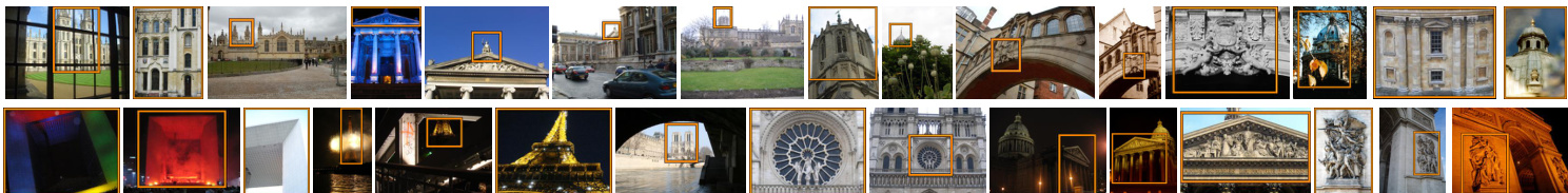
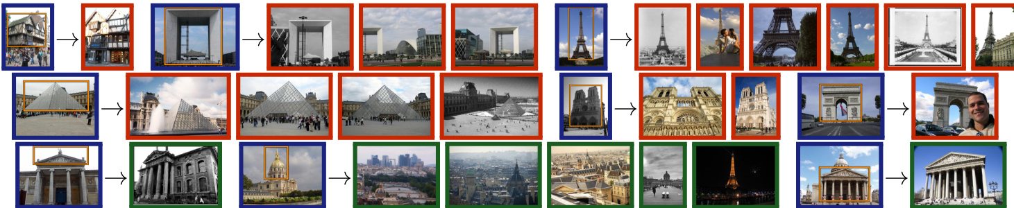
Figure 1. The newly added queries for ROxford(top) and RParis(bottom) datasets. Merged with the original queries, they comprise a new set of 70 queries in total. Figure 2. Examples of extreme labeling mistakes in the original labeling. We show the query (blue) image and the associated databas images that were originally marked as negative (red) or positive (green). Best viewed in color.
图 1: ROxford(上)和RParis(下)数据集新增的查询图像。与原始查询合并后,共计形成包含70个查询的新集合。
图 2: 原始标注中极端错误的示例。我们展示查询(蓝色)图像及原被标记为负样本(红色)或正样本(绿色)的关联数据库图像。建议彩色查看。
Hard: The image depicts the query landmark, but with viewing conditions that are difficult to match with the query. The depicted (side of the) landmark is recognizable without any contextual visual information. • Unclear: (a) The image possibly depicts the landmark in question, but the content is not enough to make a certain guess about the overlap with the query region, or context is needed to clarify. (b) The image depicts a different side of a partially symmetric building, where the symmetry is significant and disc rim i native enough. • Negative: The image is not satisfying any of the previous conditions. For instance, it depicts a different side of the landmark compared to that of the query, with no disc rim i native symmetries. If the image has any physical overlap with the query, it is never negative, but rather unclear, easy, or hard according to the above.
困难:图像描绘了查询地标,但视角条件难以与查询匹配。无需任何上下文视觉信息即可识别所描绘的地标(侧面)。
• 不明确:(a) 图像可能描绘了目标地标,但内容不足以确定与查询区域的重叠程度,或需要上下文来澄清。(b) 图像描绘了部分对称建筑的另一侧,其对称性显著且具有足够区分度。
• 负面:图像不满足上述任何条件。例如,与查询相比,它描绘了地标的另一侧,且无区分性对称特征。若图像与查询存在物理重叠,则根据上述标准归为不明确、简单或困难,而非负面。
Labeling step 3: Refinement. For each query group, each image in the list of potential positives has been assigned a five-tuple of labels, one per annotator. We perform majority voting in two steps to define the final label. The first step is voting for ${{\mathrm{easy}},{\mathrm{hard}}}$ , ${{\mathrm{unclear}}}$ , or ${{\mathrm{negative}}}$ , grouping easy and hard together. In case majority goes to ${\mathrm{easy},\mathrm{hard}}$ , the second step is to decide which of the two. Draws of the first step are assigned to unclear, and of the second step to hard. Illustrative examples are (EEHUU) $\rightarrow$ E, $(\mathrm{EHUUN})\to\mathrm{U}$ , and $(\mathrm{HHUNN})\to\mathrm{U}$ . Finally, for each query group, we inspect images by descending label entropy to make sure there are no errors.
标注步骤3:精修。对于每个查询组,潜在正例列表中的每张图像都被分配了一个五元组标签(每位标注者一个)。我们通过两步多数投票来确定最终标签:第一步在{简单(easy)、困难(hard)}、{不明确(unclear)}或{负例(negative)}之间投票,其中简单和困难归为一组。若多数票属于{easy,hard},则第二步决定具体是二者中的哪一个。第一步平局时归为不明确,第二步平局时归为困难。示例包括(EEHUU)→E、(EHUUN)→U以及(HHUNN)→U。最后,对于每个查询组,我们按标签熵降序检查图像以确保无误。
Revisited datasets: Oxford and Paris. Images from which the queries are cropped are excluded from the evaluation dataset. This way, unfair comparisons are avoided in the case of methods performing off-line preprocessing of the database [2, 14]; any preprocessing should not include any part of query images. The revisited datasets, namely, $\mathcal{R}$ Oxford and RParis, comprise 4,993 and 6,322 images respectively, after removing the 70 queries.
重新评估的数据集:Oxford和Paris。评估数据集中排除了从中裁剪查询的图像。这样可避免对数据库进行离线预处理的方法[2,14]产生不公平比较;任何预处理都不应包含查询图像的任何部分。重新评估的数据集,即$\mathcal{R}$Oxford和RParis,在移除70个查询后分别包含4,993和6,322张图像。
In Table 1, we show statistics of label transitions from the old to the new annotations. Note that errors in the original annotation that affect the evaluation, e.g. negative moving to easy or hard, are not uncommon. The transitions from junk to easy or hard are reflecting the greater challenges of the new annotation. Representative examples of extreme labeling errors of the original annotation are shown in Figure 2. In Figure 3, representative examples of easy, hard, and unclear images are presented for several queries. This will help understanding the level of challenge of each evaluation protocol listed below.
在表1中,我们展示了从旧标注到新标注的标签转换统计。需要注意的是,原始标注中影响评估的错误(例如负面样本转为简单或困难样本)并不罕见。从垃圾样本转为简单或困难样本的转换反映了新标注面临的更大挑战。图2展示了原始标注中极端标签错误的代表性案例。图3则针对多个查询展示了简单、困难和模糊图像的代表性示例,这将有助于理解下文列出的每种评估协议的挑战级别。
2.3. Evaluation protocol
2.3. 评估协议
Only the cropped regions are to be used as queries; never the full image, since the ground-truth labeling strictly considers only the visual content inside the query region.
仅将裁剪区域用作查询;切勿使用完整图像,因为真实标注严格仅考虑查询区域内的视觉内容。
The standard practice of reporting mean average precision (mAP) [33] for performance evaluation is followed. Additionally, mean precision at rank $K$ $(\mathrm{mP}@K)$ is reported. The former reflects the overall quality of the ranked list. The latter reflects the quality of the results of a search engine as they would be visually inspected by a user. More importantly, it is correlated to performance of subsequent processing steps [7, 21]. During the evaluation, positive images should be retrieved, while there is also an ignore list per query. Three evaluation setups of different difficulty are defined by treating labels (easy, hard, unclear) as positive or negative, or ignoring them:
遵循标准做法,报告平均精度均值 (mAP) [33] 进行性能评估。此外,还报告了排名 $K$ 处的平均精度 $(\mathrm{mP}@K)$。前者反映了排序列表的整体质量,后者则反映了搜索引擎结果在用户视觉检查时的质量。更重要的是,它与后续处理步骤的性能相关 [7, 21]。在评估过程中,应检索正样本图像,同时每个查询还有一个忽略列表。通过将标签(简单、困难、不明确)视为正样本、负样本或忽略它们,定义了三种不同难度的评估设置:
Easy (E): Easy images are treated as positive, while Hard and Unclear are ignored (same as Junk in [33]). • Medium (M): Easy and Hard images are treated as positive, while Unclear are ignored. Hard (H): Hard images are treated as positive, while Easy and Unclear are ignored.
简单 (E): 简单图像视为正样本,困难 (Hard) 和模糊 (Unclear) 图像被忽略 (与 [33] 中的 Junk 处理方式相同)。
中等 (M): 简单和困难图像视为正样本,模糊图像被忽略。
困难 (H): 困难图像视为正样本,简单和模糊图像被忽略。
If there are no positive images for a query in a particular setting, then that query is excluded from the evaluation.
如果在特定设置中没有查询的正样本图像,则该查询将从评估中排除。
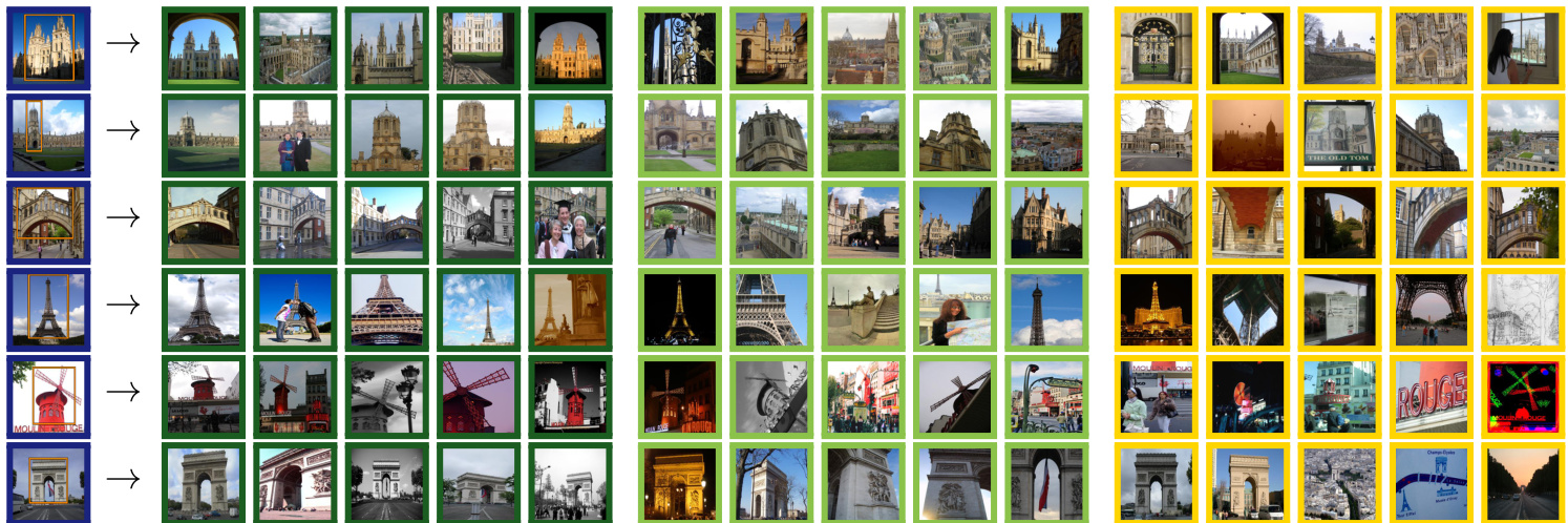
Figure 3. Sample query (blue) images and images that are respectively marked as easy (dark green), hard (light green), and unclear (yellow). Best viewed in color.
图 3: 查询图像(蓝色)示例及分别标记为简单(深绿)、困难(浅绿)和不确定(黄色)的图像。建议彩色查看。
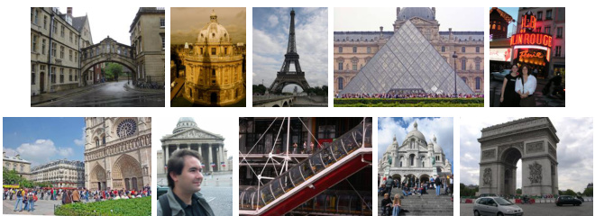
Figure 4. Sample false negative images in Oxford100k.
图 4: Oxford100k数据集中的假阴性样本图像。
The original annotation and evaluation protocol is closest to our Easy setup. Even though this setup is now trivial for the best performing methods, it can still be used for evaluation of e.g. near duplicate detection or retrieval with ultra short codes. The other setups, Medium and Hard, are challenging and even the best performing methods achieve relatively low scores. See Section 4 for details.
原始标注和评估协议最接近我们的简易设置 (Easy setup)。尽管这一设置对性能最佳的方法来说已微不足道,但仍可用于评估近重复检测或超短代码检索等任务。中等 (Medium) 和困难 (Hard) 设置则具有挑战性,即使表现最佳的方法得分也相对较低。详见第4节。
2.4. Distractor set 1M
2.4. 干扰项集 1M
Large scale experiments on Oxford and Paris dataset are commonly performed with the accompanying distractor set of 100k images, namely Oxford100k [33]. Recent results [14, 13] show that the performance only slightly degrades by adding Oxford100k in the database compared to a small-scale setting. Moreover, it is not manually cleaned and, as a consequence, Oxford and Paris landmarks are depicted in some of the distractor images (see Figure 4), hence adding further noise to the evaluation procedure.
在Oxford和Paris数据集上进行的大规模实验通常使用附带的10万张干扰图像集(即Oxford100k [33])。近期研究[14, 13]表明,与小型设置相比,在数据库中添加Oxford100k仅会轻微降低性能。此外,该干扰集未经过人工清理,因此部分干扰图像中仍包含Oxford和Paris地标(见图4),这给评估过程引入了额外噪声。
Larger distactor sets are used in the literature [33, 34, 16, 44] but none of them are standardized to provide a testbed for direct large scale comparison nor are they manually cleaned [16]. Some of the distractor sets are also biased, since they contain images of different resolution than the Oxford and Paris datasets.
文献中使用了更大的干扰项集 [33, 34, 16, 44],但它们均未经过标准化处理以提供直接大规模比较的测试基准,也未经过人工清洗 [16]。部分干扰项集还存在偏差,因为它们包含的图像分辨率与Oxford和Paris数据集不同。
We construct a new distractor set with exactly 1,001,001 high-resolution $(1024\times768)$ images, which we refer to as $\mathcal{R}1\mathbf{M}$ dataset. It is cleaned by a semi-automatic process. We automatically pick hard images for a number of state-of-theart methods, resulting in a challenging large scale setup.
我们构建了一个全新的干扰项集,包含1,001,001张高分辨率 $(1024\times768)$ 图像,称为 $\mathcal{R}1\mathbf{M}$ 数据集。该数据集通过半自动化流程进行清洗,并针对多种前沿方法自动筛选出困难样本,从而形成具有挑战性的大规模实验设置。
YFCC100M and semi-automatic cleaning. We randomly choose 5M images with GPS information from YFCC100M dataset [43]. Then, we exclude UK, France, and Las Vegas; the latter due to the Eiffel Tower and Arc de Triomphe replicas. We end up with roughly 4.1M images that are available for downloading in high resolution. We rank images with the same search tool as used in labeling step 1. Then, we manually inspect the top 2k images per landmark, and remove those depicting the query landmarks (faulty GPS, toy models, and paintings/photographs of landmarks). In total, we find 110 such images.
YFCC100M与半自动清洗。我们从YFCC100M数据集[43]中随机选取500万张含GPS信息的图像,随后排除英国、法国和拉斯维加斯的数据(后者的剔除原因是埃菲尔铁塔和凯旋门的复制品)。最终获得约410万张可下载的高分辨率图像。使用与标注步骤1相同的搜索工具对图像进行排序,随后人工检查每个地标的前2000张图像,剔除包含查询地标的错误数据(GPS错误、玩具模型以及地标的绘画/照片)。共发现110张此类问题图像。
Un-biased mining of distracting images. We propose a way to keep the most challenging 1M out of the 4.1M images. We perform all 70 queries into the 4.1M database with a number of methods. For each query and for each distractor image we count the fraction of easy or hard images that are ranked after it. We sum these fractions over all queries of ROxford and RParis and over different methods, resulting in a measurement of how distracting each distractor image is. We choose the set of 1M most distracting images and refer to it as the ${\mathcal{R}}1\mathbf{M}$ distractor set.
无偏见的干扰图像挖掘。我们提出了一种方法,从410万张图像中筛选出最具挑战性的100万张。通过多种方法对410万数据库执行全部70次查询,针对每个查询和每张干扰图像,统计排在它之后的简单或困难图像比例。我们将这些比例在ROxford和RParis的所有查询及不同方法上求和,从而量化每张干扰图像的干扰程度。最终选出最具干扰性的100万张图像,称为${\mathcal{R}}1\mathbf{M}$干扰集。
Three complementary retrieval methods are chosen to compute this measurement. These are fine-tuned ResNet with GeM pooling [37], pre-trained (on ImageNet) AlexNet with MAC pooling [38], and ASMK [46]. More details on these methods are given in Section 3. Finally, we perform a sanity check to show that this selection process is not significantly biased to distract only those 3 methods. This includes two additional methods, VLAD [18] and finetuned ResNet with R-MAC pooling by Gordo et al. [10]. As shown in Table 2, the performance on the hardest 1M distractors is hardly affected whether one of those additional methods participates or not in the selection process. This suggests that the mining process is not biased towards particular methods.
我们选择了三种互补的检索方法来计算这一指标:采用GeM池化的微调ResNet [37]、基于ImageNet预训练的MAC池化AlexNet [38]以及ASMK [46]。这些方法的详细说明见第3节。最后我们通过验证实验表明,该筛选过程不会显著偏袒那三种方法——我们额外测试了VLAD [18]和Gordo等人提出的R-MAC池化微调ResNet [10]。如表2所示,无论是否加入这两种额外方法参与筛选,在100万最难干扰项上的性能表现几乎不受影响,说明挖掘过程不存在方法偏好性。
Table 2 also shows that the distractor set we choose (version 1M (1,2,3) in the Table) is much harder than a random 1M subset and nearly as hard as all 4M distractor images. Example images from the set ${\mathcal{R}}1\mathbf{M}$ are shown in Figure 5.
表 2 还显示,我们选择的干扰项集 (表格中的 version 1M (1,2,3) ) 比随机 1M 子集要难得多,且几乎与全部 4M 干扰图像难度相当。图 5 展示了来自 ${\mathcal{R}}1\mathbf{M}$ 集合的示例图像。
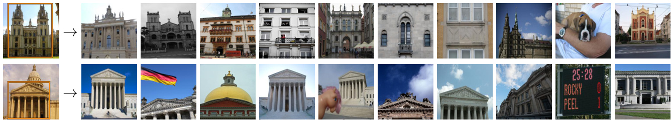
Figure 5. The most distracting images per query for two queries.
图 5: 两个查询中每个查询最分散注意力的图像。
3. Extensive evaluation
3. 广泛评估
We evaluate a number of state-of-the-art approaches on the new benchmark and offer a rich testbed for future comparisons. We list them in this section and they belong to two main categories, namely, classical retrieval approaches using local features and CNN-based methods producing global image descriptors.
我们在新基准上评估了多种先进方法,为未来的比较提供了丰富的测试平台。本节列举的这些方法主要分为两大类:使用局部特征的经典检索方法和生成全局图像描述符的基于CNN的方法。
3.1. Local-feature-based methods
3.1. 基于局部特征的方法
Methods based on local invariant features [25, 26] and the Bag-of-Words (BoW) model [41, 33, 7, 34, 6, 27, 47, 4, 52, 54, 42] were dominating the field of image retrieval until the advent of CNN-based approaches [38, 3, 48, 20, 1, 10, 37, 28, 51]. A typical pipeline consists of invariant local feature detection [26], local descriptor extrac- tion [25], quantization with a visual codebook [41], typ- ically created with $k$ -means, assignment of descriptors to visual words and finally descriptor aggregation in a single embedding [19, 32] or individual feature indexing with an inverted file structure [45, 33, 31]. We consider state-ofthe-art methods from both categories. In particular, we use up-right hessian-affine (HesAff) features [31], RootSIFT (rSIFT) descriptors [2], and create the codebooks on the landmark dataset from [37], same as the one used for the whitening of CNN-based methods. Note that we always crop the queries according to the defined region and then perform any processing to be directly comparable to CNNbased methods.
基于局部不变特征的方法 [25, 26] 和词袋模型 (BoW) [41, 33, 7, 34, 6, 27, 47, 4, 52, 54, 42] 在基于 CNN 的方法 [38, 3, 48, 20, 1, 10, 37, 28, 51] 出现之前一直主导着图像检索领域。典型流程包括:局部不变特征检测 [26]、局部描述子提取 [25]、使用视觉词典进行量化 [41](通常通过 $k$ 均值方法生成)、将描述子分配到视觉单词,最后通过单一嵌入 [19, 32] 进行描述子聚合或采用倒排文件结构 [45, 33, 31] 进行独立特征索引。我们综合考量了两类方法中的前沿技术,具体采用直立海森仿射 (HesAff) 特征 [31]、RootSIFT (rSIFT) 描述子 [2],并在与 CNN 方法白化处理相同的地标数据集 [37] 上构建词典。需注意,我们会根据定义区域裁剪查询图像后再进行所有处理,以确保与基于 CNN 的方法具有直接可比性。
| Distractorset | ROxford | RParis | ||||||||
|---|---|---|---|---|---|---|---|---|---|---|
| 方法 | (1) | (2) | (3) | (4) | (5) | (1) | (2) | (3) | ||
| 4M | 33.3 | 11.1 | 33.2 | 33.7 | 15.6 | 40.7 | 11.4 | 30.0 | 45.4 | |
| 1M (1,2,3) 1M (1,2,3,4) | 33.9 33.7 | 11.1 11.1 | 34.8 34.8 | 33.9 33.8 | 17.4 17.5 | 44.1 43.8 | 11.8 11.8 | 31.7 31.8 | 48.1 47.7 | |
| 1M (1,2,3,5) | 33.7 | 11.1 | 34.6 | 33.9 | 17.2 | 43.5 | 11.7 | 31.4 | 47.7 | |
| 37.6 | ||||||||||
| 1M (random) | 13.7 | 37.4 | 38.9 | 20.4 | 47.3 | 16.2 | 34.2 | 53.1 |
Table 2. Performance (mAP) evaluation with the Medium protocol for different distractor sets. The methods considered are (1) Fine-tuned ResNet101 with GeM pooling [37]; (2) Offthe-shelf AlexNet with MAC pooling [38]; (3) HesAff–rSIFT– ASMK⋆ [46]; (4) Fine-tuned ResNet101 with R-MAC pooling [10]; (5) HesAff–rSIFT–VLAD [18]. The sanity check in- cludes evaluation for different distractor sets, i.e. all, hardest subset chosen by method (1,2,3), (1,2,3,4), (1,2,4,5), and a random 1M sample.
表 2: 采用Medium协议在不同干扰集下的性能(mAP)评估。评估方法包括:(1) 使用GeM池化的微调ResNet101 [37];(2) 使用MAC池化的现成AlexNet [38];(3) HesAff–rSIFT–ASMK⋆ [46];(4) 使用R-MAC池化的微调ResNet101 [10];(5) HesAff–rSIFT–VLAD [18]。完整性检查涵盖不同干扰集的评估,包括:全部样本、由方法(1,2,3)选出的最难子集、(1,2,3,4)、(1,2,4,5)以及随机100万样本。
We additionally follow the same BoW-based pipeline while replacing hessian-affine and RootSIFT with the deep local attentive features (DELF) [30]. The default extraction approach is followed (i.e. at most 1000 features per image), but we reduce the descriptor dimensionality to 128 and not to 40 to be comparable to RootSIFT. This variant is a bridge between classical approaches and deep learning.
此外,我们沿用相同的基于词袋模型(BoW)的流程,但将hessian-affine和RootSIFT替换为深度局部注意力特征(DELF) [30]。遵循默认提取方法(即每张图像最多提取1000个特征),但我们将描述符维度降至128而非40,以保持与RootSIFT的可比性。该变体是经典方法与深度学习之间的桥梁。
VLAD. The Vector of Locally Aggregated Descriptors [18] (VLAD) is created by first-order statistics of the local descriptors. The residual vectors between descriptors and the closest centroid are aggregated w.r.t. a codebook whose size is 256 in our experiments. We reduce its dimensionality down to 2048 with PCA, while square-root normalization is also used [15].
VLAD。局部聚合描述子向量 (VLAD) [18] 是通过局部描述子的一阶统计量构建的。在实验中,我们使用大小为256的码本对描述子与其最近质心之间的残差向量进行聚合,并通过PCA (主成分分析) 将其维度降至2048,同时采用平方根归一化 [15]。
$\mathbf{SMK^{\star}}$ . The binarized version of the Selective Match Kernel [46] $(\mathbf{S}\mathbf{M}\mathbf{K}^{\star})$ ), a simple extension of the Hamming Em- bedding [16] (HE) technique, uses an inverted file structure to separately indexes binarized residual vectors while it performs the matching with a selective monomial kernel function. The codebook size is 65,536 in our experiments, while burstiness normalization [17] is always used. Multiple assignment to three nearest words is used on the query side, while the hamming distance threshold is set to 52 out of 128 bits. The rest are the default parameters.
$\mathbf{SMK^{\star}}$。选择性匹配核[46]的二值化版本$(\mathbf{S}\mathbf{M}\mathbf{K}^{\star})$ )是汉明嵌入[16] (HE) 技术的简单扩展,它使用倒排文件结构分别索引二值化残差向量,同时通过选择性单项核函数进行匹配。我们的实验中码本大小为65,536,且始终使用突发性归一化[17]。查询端采用三近邻词多重分配策略,汉明距离阈值设置为128位中的52位。其余参数保持默认值。
$\mathbf{ASMK^{\star}}$ . The binarized version of the Aggregated Selective Match Kernel [46] $(\mathbf{ASMK}^{\star})$ ) is an extension of $\mathrm{SMK^{\star}}$ that jointly encodes local descriptors that are assigned to the same visual word and handles the burstiness phenomenon. Same para me tri z ation as $\mathrm{SMK^{\star}}$ is used.
$\mathbf{ASMK^{\star}}$。聚合选择性匹配核 [46] 的二进制版本 $(\mathbf{ASMK}^{\star})$ ) 是 $\mathrm{SMK^{\star}}$ 的扩展,它联合编码分配到同一视觉词的局部描述符,并处理突发性现象。参数化方式与 $\mathrm{SMK^{\star}}$ 相同。
SP. Spatial verification (SP) is known to be crucial for particular object retrieval [33] and is performed with the RANSAC algorithm [8]. It is applied on the 100 top-ranked images, as these are formed by a first filtering step, e.g. the $\mathrm{SMK^{\star}}$ or ${\mathrm{ASMK}}^{\star}$ method. Its result is the number of inlier correspondences, which is one of the most intuitive similarity measures and allows to detect true positive images. To assume that an image is spatially verified, we require 5 inliers with ${\mathrm{ASMK}}^{\star}$ and 10 with other methods.
SP. 空间验证 (SP) 对特定物体检索至关重要 [33],通常通过 RANSAC 算法 [8] 实现。该步骤作用于前 100 张候选图像(由 $\mathrm{SMK^{\star}}$ 或 ${\mathrm{ASMK}}^{\star}$ 等方法初步筛选得出),其输出结果为内点匹配数——这是最直观的相似度度量之一,可有效识别真阳性图像。我们设定空间验证通过标准为:使用 ${\mathrm{ASMK}}^{\star}$ 时需至少 5 个内点,其他方法需 10 个内点。
HQE. Query expansion (QE), firstly introduced by Chum et al. [7] in the visual domain, typically uses spatial verification to select true positive among the top retrieved result and issues an enhanced query including the verified images. Hamming Query Expansion [47] (HQE) is combining QE with HE. We use same soft assignment as $\mathrm{SMK^{\star}}$ and the default parameters.
HQE。查询扩展 (query expansion, QE) 最初由 Chum 等人 [7] 在视觉领域提出,通常通过空间验证从检索结果中筛选出真实正例,并生成包含已验证图像的增强查询。汉明查询扩展 [47] (HQE) 将 QE 与 HE 相结合。我们采用与 $\mathrm{SMK^{\star}}$ 相同的软分配策略及默认参数。
3.2. CNN-based global descriptor methods
3.2. 基于CNN的全局描述符方法
We list different aspects of a CNN-based method for image retrieval, which we later combine to form different baselines that exist in the literature.
我们列出基于CNN(卷积神经网络)的图像检索方法的不同方面,后续将组合这些方面以构建文献中存在的不同基线方法。
CNN architectures. We include 3 highly influential CNN architectures, namely AlexNet [22], VGG-16 [40], and ResNet101 [12]. They have different number of layers, complexity, and also produce descriptors of different dimens ional it y (256, 512, and 2048, respectively).
CNN架构。我们选取了3种极具影响力的CNN架构:AlexNet [22]、VGG-16 [40]和ResNet101 [12]。这些架构具有不同的层数、复杂度,并分别生成不同维度的描述符(256、512和2048维)。
Pooling. A common practice is to consider a convolutional feature map and perform a pooling mechanism to construct a global image descriptor. We consider max-pooling (MAC) [38, 48], sum-pooling (SPoC) [3], weighted sum-pooling (CroW) [20], regional max-pooling (R-MAC) [48], generalized mean-pooling (GeM) [37], and NetVLAD pooling [1]. The pooling is always applied on the last convolutional feature map.
池化。常见的做法是考虑卷积特征图并执行池化机制来构建全局图像描述符。我们考虑了最大池化 (MAC) [38, 48]、求和池化 (SPoC) [3]、加权求和池化 (CroW) [20]、区域最大池化 (R-MAC) [48]、广义平均池化 (GeM) [37] 以及 NetVLAD 池化 [1]。池化始终应用于最后一个卷积特征图。
Multi-scale. The input image is resized to a maximum $1024\times1024$ size. Then, three re-scaled versions with scaling factor of 1, $^{1}/{\sqrt{2}}$ , and $^1/2$ are fed to the network. Fi- nally, the resulting descriptors are combined into a single descriptor by average pooling [10] for all methods, except for GeM where generalized-mean pooling is used [37]. This is shown to improve the performance of the CNN-based descriptors [10, 37].
多尺度。输入图像被调整至最大 $1024\times1024$ 尺寸,随后生成缩放因子分别为1、$^{1}/{\sqrt{2}}$ 和 $^1/2$ 的三个重缩放版本输入网络。最终通过平均池化 [10] 将所有方法生成的描述符合并为单一描述符(GeM方法除外,其采用广义均值池化 [37])。研究表明该策略能提升基于CNN的描述符性能 [10, 37]。
Off-the-shelf vs. retrieval fine-tuning. Networks that are pre-trained on ImageNet [39] (off-the-shelf) are directly applicable on image retrieval. Moreover, we consider the following cases of fine-tuning for the task. Radenovic et al. [36] fine-tune a network with landmarks photos using contrastive loss [11]. This is available with MAC [36] and GeM pooling [37]. Similarly, Gordo et al. [10] fine-tune R-MAC pooling with landmark photos and triplet loss [50]. Finally, NetVLAD [1] is fine-tuned using street-view images and GPS information.
现成模型与检索微调对比。在ImageNet [39]上预训练的现成网络可直接应用于图像检索。此外,我们针对该任务考虑了以下微调方案:Radenovic等人 [36] 使用地标照片和对比损失 [11] 对网络进行微调,该方法支持MAC [36] 和GeM池化 [37];类似地,Gordo等人 [10] 采用地标照片和三元组损失 [50] 对R-MAC池化进行微调;NetVLAD [1] 则使用街景图像和GPS信息进行微调。
Descriptor whitening is known to be essential for such descriptors. We use the same landmark dataset [37] to learn the whitening for all methods. We use PCA whitening [15, 3] for all the off-the-shelf networks, and supervised whitening with SfM labels [24, 36] for all the fine-tuned ones. One exception is the tuning that includes the whitening in the network [10].
描述符白化 (whitening) 是此类描述符的关键步骤。我们使用相同的地标数据集 [37] 为所有方法学习白化参数。对于现成网络采用 PCA 白化 [15, 3],对于微调网络则采用基于 SfM 标签的监督式白化 [24, 36]。唯一例外是将白化层集成到网络中的调优方法 [10]。
Query Expansion is directly applicable on top of global CNN-based descriptors. More specifically, we use $\alpha$ query expansion [37] $(\alpha\mathrm{QE})$ and diffusion [14] (DFS).
查询扩展可直接应用于基于全局CNN的描述符之上。具体而言,我们使用 $\alpha$ 查询扩展 [37] $(\alpha\mathrm{QE})$ 和扩散 [14] (DFS)。
Table 3. Performance (mAP) on Oxford (Oxf) and Paris (Par) with the original annotation, and Oxford and Paris with the newly proposed annotation with three different protocol setups: Easy (E), Medium (M), Hard (H).
表 3: 采用原始标注的Oxford (Oxf)和Paris (Par)数据集性能(mAP),以及采用新提出的三种不同协议设置(Easy (E)、Medium (M)、Hard (H))标注的Oxford和Paris数据集性能。
| 方法 | Oxf | ROxford | Par | RParis | ||||
|---|---|---|---|---|---|---|---|---|
| E | M | H | E | M | H | |||
| HesAff-rSIFT-SMK* R-[O]-R-MAC R-[37]-GeM R-[37]-GeM+DFS | 78.1 78.3 87.8 | 74.1 74.2 | 59.4 49.8 | 35.4 18.5 | 74.6 90.9 | 80.6 89.9 | 59.0 74.0 | 31.2 52.1 |
| 方法 | 内存 (GB) | 提取时间 (秒) | 搜索时间 (秒) |
|---|---|---|---|
| GPU | CPU | ||
| HesAff-rSIFT-ASMK*+SP | 62.0 | n/a + 0.06 | 1.08 +2.35 |
| DELF-ASMK*+SP | 10.3 | 0.41 + 0.01 | n/a + 0.54 |
| A-[37]-GeM | 0.96 | 0.12 | 1.99 |
| V-[37]-GeM | 1.92 | 0.23 | 31.11 |
| R-[37]-GeM | 7.68 | 0.37 | 14.51 |
Table 4. Time and memory measurements. Extraction time on a single thread GPU (Tesla P100) / CPU (Intel Xeon CPU E5-2630 $\mathrm{v}2~@~2.60\mathrm{GHz})$ per image of size $1024\mathrm{x}768$ , the memory requirements and the search time (single thread CPU) reported for the database of $\mathcal{R}\mathrm{Oxford+}\mathcal{R}\mathrm{lM}$ images. Feature extraction $^+$ visual word assignment is reported for ${\mathrm{ASMK}}^{\star}$ . SP: Geometry information is loaded from the disk and the loading time is included in search time. We did not consider geometry quantization [31].
表 4: 时间和内存测量。单线程 GPU (Tesla P100) / CPU (Intel Xeon CPU E5-2630 $\mathrm{v}2~@~2.60\mathrm{GHz}$) 对尺寸为 $1024\mathrm{x}768$ 的单张图像提取时间,以及 $\mathcal{R}\mathrm{Oxford+}\mathcal{R}\mathrm{lM}$ 图像数据库的内存需求和搜索时间 (单线程 CPU)。${\mathrm{ASMK}}^{\star}$ 报告了特征提取 $^+$ 视觉词分配。SP: 几何信息从磁盘加载,加载时间包含在搜索时间内。我们未考虑几何量化 [31]。
4. Results
4. 结果
We report a performance comparison between the old and the revisited datasets. Additionally, we provide an extensive evaluation of the state-of-the-art methods on the revisited dataset, with and without the new large-scale distractor set, setting up a testbed for future comparisons.
我们报告了新旧数据集之间的性能对比。此外,我们对当前最先进方法在修订版数据集上进行了全面评估(包含和不包含新的大规模干扰集),为未来比较建立了测试基准。
The evaluation includes local feature-based approaches (see Section 3.1 for details and abbreviations), referred to by the combination of local feature type and representation method, e.g. HesAff–rSIFT–ASMK⋆. CNN-based global descriptors are denoted with the following abbreviations. Network architectures are AlexNet (A), VGG-16 (V), and ResNet101 (R). The fine-tuning options are triplet loss with GPS guided mining [1], triplet loss with spatially verified positive pairs [10], contrastive loss with mining from 3D models [36] and [37], and finally the off-the-shelf [O] networks. Pooling approaches are as listed in Section 3.2. For instance, ResNet101 with GeM pooling that is fine-tuned with contrastive loss and the training dataset by Radenovic et al. [37] is referred to as R–[37]–GeM.
评估包括基于局部特征的方法(详见第3.1节及其缩写),通过局部特征类型与表示方法的组合来指代,例如HesAff–rSIFT–ASMK⋆。基于CNN的全局描述符采用以下缩写表示:网络架构为AlexNet (A)、VGG-16 (V)和ResNet101 (R)。微调选项包括采用GPS引导挖掘的三元组损失[1]、空间验证正样本对的三元组损失[10]、基于3D模型挖掘的对比损失[36]和[37],以及现成的[O]网络。池化方法如第3.2节所列。例如,采用GeM池化的ResNet101,使用Radenovic等人[37]的训练数据集通过对比损失微调,记作R–[37]–GeM。
Revisited vs. original. We compare the performance when evaluated on the original datasets, and the revisited annotation with the new protocols. The results for four representative methods are presented in Table 3. The old setup appears to be close to the new Easy setup, while Medium and Hard appear to be more challenging. We observe that the performance of the Easy setup is nearly saturated and, therefore, do not use it but only evaluate Medium and Hard setups in the subsequent experiments.
重评估 vs. 原始数据。我们比较了在原始数据集上的评估性能,以及采用新协议重新标注后的结果。四种代表性方法的结果如表 3 所示。旧设置似乎接近于新的简单 (Easy) 设置,而中等 (Medium) 和困难 (Hard) 设置则更具挑战性。我们观察到简单设置的性能已接近饱和,因此在后续实验中仅评估中等和困难设置。
Table 5. Performance evaluation (mAP, $\mathrm{mP}@10,$ ) on ROxford (ROxf) and RParis (RPar) without and with ${\cal{R}}1\mathbf{M}$ distract or s. We report results with the revisited annotation, using Medium and Hard evaluation protocols. We use a color-map that is normalized according to the minimum (white) and maximum (green / orange) value per column.
| 方法 | ROxf mAP | ROxf mP@10 | ROxf+R1M mAP | ROxf+R1M mP@10 | RPar mAP | RPar mP@10 | RPar+R1M mAP | RPar+R1M mP@10 | ROxf mAP | ROxf mP@10 | ROxf+R1M mAP | ROxf+R1M mP@10 | RPar mAP | RPar mP@10 | RPar+R1M mAP | RPar+R1M mP@10 |
|---|---|---|---|---|---|---|---|---|---|---|---|---|---|---|---|---|
| HesAff-rSIFT-VLAD | 33.9 | 54.9 | 17.4 | 34.8 | 43.6 | 90.9 | 19.6 | 76.1 | 13.2 | 18.1 | 5.6 | 7.0 | 17.5 | 50.7 | 3.3 | 21.1 |
| HesAff-rSIFT-SMK* | 59.4 | 83.6 | 35.8 | 64.6 | 59.0 | 97.4 | 34.1 | 89.1 | 35.4 | 53.7 | 16.4 | 27.7 | 31.2 | 72.6 | 10.5 | 47.6 |
| HesAff-rSIFT-ASMK* | 60.4 | 85.6 | 45.0 | 76.0 | 61.2 | 97.9 | 42.0 | 95.3 | 36.4 | 56.7 | 25.7 | 42.1 | 34.5 | 80.6 | 16.5 | 63.4 |
| HesAff-rSIFT-SMK*+SP | 60.6 | 86.1 | 46.8 | 79.6 | 61.4 | 97.9 | 42.3 | 95.3 | 36.7 | 57.0 | 26.9 | 45.3 | 35.0 | 81.7 | 16.8 | 65.3 |
| HesAff-rSIFT-ASMK*+SP | 87.9 | 53.8 | 81.1 | 76.9 | 99.3 | 57.3 | 98.3 | 43.1 | 62.4 | 31.2 | 50.7 | 55.4 | 93.4 | 26.4 | 75.7 | |
| DELF-ASMK*+SP | 67.8 | 44.7 | 14.1 | 28.3 | 47.3 | 88.6 | 18.7 | 69.4 | 8.8 | 15.5 | 3.5 | 5.1 | 23.1 | 61.6 | 4.1 | |
| A-[O]-MAC | 28.3 | 33.8 | 51.2 | 16.3 | 32.4 | 52.7 | 90.1 | 23.8 | 78.1 | 10.4 | 16.7 | 3.9 | 6.3 | 26.0 | 68.0 | 5.5 |
| A-[O]-GeM | 41.3 | 62.1 | 23.9 | 43.0 | 56.4 | 92.9 | 29.6 | 85.4 | 17.8 | 28.2 | 8.4 | 11.9 | 28.7 | 69.3 | 8.5 | 31.6 |
| A-[37]-GeM | 43.3 | 62.1 | 24.2 | 42.8 | 58.0 | 91.6 | 29.9 | 84.6 | 17.1 | 26.2 | 9.4 | 11.9 | 29.7 | 67.6 | 8.4 | 39.6 |
| V-[O]-MAC | 37.8 | 57.8 | 21.8 | 39.7 | 59.2 | 93.3 | 33.6 | 87.1 | 14.6 | 27.0 | 7.4 | 11.9 | 35.9 | 78.4 | 13.2 | 54.7 |
| V-[O]-SPoC | 38.0 | 54.6 | 17.1 | 33.3 | 59.8 | 93.0 | 30.3 | 83.0 | 11.4 | 20.9 | 0.9 | 2.9 | 32.4 | 69.7 | 7.6 | 30.6 |
| V-[O]-CroW | 41.4 | 58.8 | 22.5 | 40.5 | 62.9 | 94.4 | 34.1 | 87.1 | 13.9 | 25.7 | 3.0 | 6.6 | 36.9 | 77.9 | 10.3 | 45.1 |
| V-[O]-GeM | 40.5 | 60.3 | 25.4 | 45.6 | 63.2 | 94.6 | 37.5 | 88.6 | 15.7 | 28.6 | 7.6 | 12.1 | 38.8 | 79.0 | 14.2 | 55.9 |
| V-[O]-R-MAC | 42.5 | 62.8 | 21.7 | 40.3 | 66.2 | 95.4 | 39.9 | 88.9 | 12.0 | 26.1 | 1.7 | 5.8 | 40.9 | 77.1 | 14.8 | 54.0 |
| V-[1]-NetVLAD | 37.1 | 56.5 | 20.7 | 37.1 | 59.8 | 94.0 | 31.8 | 85.7 | 13.8 | 23.3 | 6.0 | 8.4 | 35.0 | 73.7 | 11.5 | 46.6 |
| V-[36]-MAC | 58.4 | 81.1 | 39.7 | 68.6 | 66.8 | 97.7 | 42.4 | 92.6 | 30.5 | 48.0 | 17.9 | 27.9 | 42.0 | 82.9 | 17.7 | 63.7 |
| V-[37]-GeM | 61.9 | 82.7 | 42.6 | 68.1 | 69.3 | 97.9 | 45.4 | 94.1 | 33.7 | 51.0 | 19.0 | 29.4 | 44.3 | 83.7 | 19.1 | 64.9 |
| R-[O]-MAC | 41.7 | 65.0 | 24.2 | 43.7 | 66.2 | 96.4 | 40.8 | 93.0 | 18.0 | 32.9 | 5.7 | 14.4 | 44.1 | 86.3 | 18.2 | 67.7 |
| R-[O]-SPoC | 39.8 | 61.0 | 21.5 | 40.4 | 69.2 | 96.7 | 41.6 | 92.0 | 12.4 | 23.8 | 2.8 | 5.6 | 44.7 | 78.0 | 15.3 | 54.4 |
| R-[O]-CroW | 42.4 | 61.9 | 21.2 | 39.4 | 70.4 | 97.1 | 42.7 | 92.9 | 13.3 | 27.7 | 3.3 | 9.3 | 47.2 | 83.6 | 16.3 | 61.6 |
| R-[O]-GeM | 45.0 | 66.2 | 25.6 | 45.1 | 70.7 | 97.0 | 46.2 | 94.0 | 17.7 | 32.6 | 4.7 | 13.4 | 48.7 | 88.0 | 20.3 | 70.4 |
| R-[O]-R-MAC | 49.8 | 68.9 | 29.2 | 48.9 | 74.0 | 97.7 | 49.3 | 93.7 | 18.5 | 32.2 | 4.5 | 13.0 | 52.1 | 87.1 | 21.3 | 67.4 |
| R-[37]-GeM | 64.7 | 84.7 | 45.2 | 71.7 | 77.2 | 98.1 | 52.3 | 95.3 | 38.5 | 53.0 | 19.9 | 34.9 | 56.3 | 89.1 | ||
| R-[10]-R-MAC | 60.9 | 78.1 | 39.3 | 62.1 | 78.9 | 96.9 | 54.8 | 93.9 | 32.4 | 50.0 | 12.5 | 24.9 | 59.4 | 86.1 | 24.7 | 28.0 |
表 5. ROxford (ROxf) 和 RParis (RPar) 在有/无 ${\cal{R}}1\mathbf{M}$ 干扰项时的性能评估 (mAP, $\mathrm{mP}@10$)。我们使用修订后的标注报告结果,采用Medium和Hard评估协议。颜色映射根据每列的最小值(白色)和最大值(绿色/橙色)进行归一化。
State of the art evaluation. We perform an extensive evaluation of the state-of-the-art methods for image retrieval. We present time/memory measurements in Table 4 and performance results in Table 5. We additionally show the average precision (AP) per query for a set of representative methods in Figures 6 and 7, for Oxford and $\mathcal{R}$ Paris, respectively. The representative set covers the progress of methods over time in the task of image retrieval. In the evaluation, we observe that there is no single method achieving the highest score on every protocol per dataset. Localfeature-based methods perform very well on ROxford, especially at large scale, achieving state-of-the-art performance, while CNN-based methods seem to dominate on $\mathcal{R}$ Paris. We observe that BoW-based classical approaches are still not obsolete, but their improvement typically comes at significant additional cost. Recent CNN-based local features, i.e. DELF, reduce the number of features and improve the performance at the same time.
最新技术评估。我们对图像检索领域的最新技术方法进行了全面评估。表4展示了时间/内存测量结果,表5呈现了性能指标。此外,图6和图7分别展示了牛津数据集和$\mathcal{R}$巴黎数据集上代表性方法的每查询平均精度(AP)。这组代表性方法涵盖了图像检索任务中技术随时间发展的进程。评估发现,没有单一方法能在每个数据集的全部评测协议上均取得最高分。基于局部特征的方法在ROxford数据集表现优异(尤其在大规模场景下达到最优性能),而基于CNN的方法则在$\mathcal{R}$Paris数据集占据优势。我们注意到基于BoW的经典方法仍未过时,但其性能提升通常伴随显著额外成本。基于CNN的最新局部特征方法(如DELF)在减少特征数量的同时提升了性能。
CNN fine-tuning consistently brings improvements over the off-the-shelf networks. The new protocols make it clear that improvements are needed at larger scale and the hard setup. Many images are not retrieved, while the top 10 results mostly contain false positives. Interestingly, we observe that query expansion approaches (e.g. diffusion) degrade the performance of queries with few relevant images (see Figures 6 and 7). This phenomenon is more pronounced in the revisited datasets, where the the query images are removed from the preprocessing. We did not include separate regional representation and indexing [38], which is previously shown to be beneficial. Preliminary experiments with ResNet and GeM pooling show that it does not deliver improvements that are significant enough to justify the additional memory and complexity cost.
CNN微调始终能带来优于现成网络的改进效果。新协议明确表明,需要在大规模和困难场景下进行改进。许多图像未被检索到,而前10个结果大多包含误报。有趣的是,我们观察到查询扩展方法(如扩散法)会降低相关图像较少的查询性能(见图6和图7)。这种现象在修订版数据集中更为明显,因为查询图像在预处理阶段已被移除。我们未采用单独的区域表示和索引方法[38],尽管先前研究已证明其有效性。使用ResNet和GeM池化的初步实验表明,其带来的改进效果不足以抵消额外的内存和复杂度开销。
The best of both worlds. The new dataset and protocols reveal space for improvement by CNN-based global descriptors in cases where local features are still better. Diffusion performs similarity propagation by starting from the query’s nearest neighbors according to the CNN global descriptor. This inevitably includes false positives, especially in the case of few relevant images. On the other hand, local features, e.g. with $\mathrm{ASMK^{\star}}+\mathrm{SP}$ , offer a verified list of relevant images. Starting the diffusion process from geometrically verified images obtained by BoW methods combines the benefits of the two worlds. This combined approach, shown at the bottom part of Table 5, improves the performance and supports the message that both worlds have their own benefits. Of course this experiment is expensive and we perform it to merely show a possible direction to improve CNN global descriptors. There are more methods that combine CNNs and local features [53], but we focus on the results related to methods included in our evaluation.
两全其美。新数据集和协议揭示了基于CNN的全局描述符在局部特征仍占优势场景下的改进空间。扩散方法通过从CNN全局描述符得出的查询最近邻开始进行相似性传播,这不可避免地包含误匹配(尤其在相关图像较少的场景中)。而局部特征(例如采用$\mathrm{ASMK^{\star}}+\mathrm{SP}$时)能提供经过几何验证的相关图像列表。从BoW方法获得的几何验证图像启动扩散过程,可结合两种方法的优势。表5底部展示的这种组合方案提升了性能,印证了"二者各有优势"的观点。当然该实验成本较高,我们仅以此展示改进CNN全局描述符的潜在方向。现有更多结合CNN与局部特征的方法[53],但我们聚焦于评估范围内相关方法的结果。

Figure 6. Performance (AP) per query on ROxford $^+$ R1M with Medium setup. AP is shown with a bar for 8 methods. The methods, from left to right, are HesAff-rSIFT-ASMK*+SP, DELF-ASMK*+SP, DELF-HQE+SP, V-[O]-R-MAC, R-[O]-GeM, R-[37]-GeM, R-[37]-GeM+DFS, HesAff-rSIFT-ASMK*+SP $\xrightarrow{}$ R-[37]-GeM+DFS. The total number of easy and hard images is printed on each histogram. Best viewed in color.
图 6: 在 ROxford$^+$R1M 中等配置下每个查询的性能 (AP)。AP 以条形图形式展示了 8 种方法的结果。从左到右依次为:HesAff-rSIFT-ASMK*+SP、DELF-ASMK*+SP、DELF-HQE+SP、V-[O]-R-MAC、R-[O]-GeM、R-[37]-GeM、R-[37]-GeM+DFS、HesAff-rSIFT-ASMK*+SP$\xrightarrow{}$R-[37]-GeM+DFS。每个直方图上标明了简单和困难图像的总数。建议彩色查看。

Figure 7. Performance (AP) per query on RParis $+\mathbf{\mathscr{R}}1\mathbf{M}$ with Medium setup. AP is shown with a bar for 8 methods. The methods, from left to right, are HesAff-rSIFT-ASMK*+SP, DELF-ASMK*+SP, DELF-HQE+SP, V-[O]-R-MAC, R-[O]-GeM, R-[37]-GeM, R-[37]-GeM+DFS, HesAff-rSIFT-ASMK*+SP $\Rightarrow$ R-[37]-GeM+DFS. The total number of easy and hard images is printed on each histogram. Best viewed in color.
图 7: RParis $+\mathbf{\mathscr{R}}1\mathbf{M}$ 数据集中等难度设置下各查询的性能(AP)。柱状图展示了8种方法的AP值,从左至右依次为:HesAff-rSIFT-ASMK*+SP、DELF-ASMK*+SP、DELF-HQE+SP、V-[O]-R-MAC、R-[O]-GeM、R-[37]-GeM、R-[37]-GeM+DFS、HesAff-rSIFT-ASMK*+SP $\Rightarrow$ R-[37]-GeM+DFS。每个直方图上标注了简单与困难图像的总数。建议彩色查看效果。
5. Conclusions
5. 结论
We have revisited two of the most established image retrieval datasets, that were perceived as performance saturated. To make it suitable for modern image retrieval benchmarking, we address drawbacks of the original annotation. This includes new annotation for both datasets that was created with an extra attention to the reliability of the ground truth, and an introduction of 1M hard distractor set.
我们重新审视了两个最成熟的图像检索数据集,这些数据集曾被认为性能已趋饱和。为了使它们适用于现代图像检索基准测试,我们解决了原始标注的缺陷。这包括为两个数据集创建的新标注(特别关注真实标签的可靠性),以及引入100万张困难干扰图像集。
An extensive evaluation provides a testbed for future comparisons and concludes that image retrieval is still an open problem, especially at large scale and under difficult viewing conditions.
一项广泛的评估为未来比较提供了测试基准,并得出结论:图像检索仍是一个待解决的问题,尤其在大规模和复杂观察条件下。