Efficient Sequence Transduction by Jointly Predicting Tokens and Durations

高效序列转导：联合预测Token与持续时间

Abstract

摘要

This paper introduces a novel Token-andDuration Transducer (TDT) architecture for sequence-to-sequence tasks. TDT extends conventional RNN-Transducer architectures by jointly predicting both a token and its duration, i.e. the number of input frames covered by the emitted token. This is achieved by using a joint network with two outputs which are independently normalized to generate distributions over tokens and durations. During inference, TDT models can skip input frames guided by the predicted duration output, which makes them significantly faster than conventional Transducers which process the encoder output frame by frame. TDT models achieve both better accuracy and significantly faster inference than conventional Transducers on different sequence transduction tasks. TDT models for Speech Recognition achieve better accuracy and up to $2.82{\mathrm X}$ faster inference than conventional Transducers. TDT models for Speech Translation achieve an absolute gain of over 1 BLEU on the MUST-C test compared with conventional Transducers, and its inference is $2.27\mathrm{X}$ faster. In Speech Intent Classification and Slot Filling tasks, TDT models improve the intent accuracy by up to over $1%$ (absolute) over conventional Transducers, while running up to $1.28\mathrm{X}$ faster. Our implementation of the TDT model will be open-sourced with the NeMo (https: //github.com/NVIDIA/NeMo) toolkit.

本文介绍了一种用于序列到序列任务的新型Token-and-Duration Transducer (TDT)架构。TDT通过联合预测token及其持续时间(即所生成token覆盖的输入帧数)，扩展了传统RNN-Transducer架构。这是通过使用具有两个输出的联合网络实现的，这两个输出独立归一化以生成token和持续时间的分布。在推理过程中，TDT模型可以根据预测的持续时间输出跳过输入帧，这使其比传统逐帧处理编码器输出的Transducer快得多。在不同序列转导任务中，TDT模型不仅精度更高，而且推理速度显著快于传统Transducer。语音识别的TDT模型比传统Transducer精度更高，推理速度最高快$2.82{\mathrm X}$。语音翻译的TDT模型在MUST-C测试集上比传统Transducer绝对提升超过1 BLEU，推理速度快$2.27\mathrm{X}$。在语音意图分类和槽填充任务中，TDT模型将意图准确率最高提升超过$1%$(绝对值)，同时运行速度最高快$1.28\mathrm{X}$。我们的TDT模型实现将通过NeMo(https://github.com/NVIDIA/NeMo)工具包开源。

1. Introduction

1. 引言

Over the past years, automatic speech recognition (ASR) models have undergone shifts from conventional hybrid models (Jelinek, 1998; Woodland et al., 1994; Povey et al., 2011) to end-to-end ASR models, including attention-based encoder and decoder (AED) models (Chorowski et al., 2015; Chan et al., 2016), Connection is t Temporal Classification (CTC) (Graves et al., 2006), and Transducers (Graves, 2012). Those models are commonly used in academia and industry, and there exist open-source toolkits with efficient implementation for those methods, including ESPNet (Watanabe et al., 2018), NeMo (Kuchaiev et al., 2019), Espresso (Wang et al., 2019), Speech Brain (Ravanelli et al., 2021) etc.

近年来，自动语音识别 (ASR) 模型经历了从传统混合模型 (Jelinek, 1998; Woodland et al., 1994; Povey et al., 2011) 到端到端 ASR 模型的转变，包括基于注意力的编码器-解码器 (AED) 模型 (Chorowski et al., 2015; Chan et al., 2016)、连接时序分类 (CTC) (Graves et al., 2006) 以及 Transducer (Graves, 2012)。这些模型在学术界和工业界广泛应用，并有高效实现的开源工具包，如 ESPNet (Watanabe et al., 2018)、NeMo (Kuchaiev et al., 2019)、Espresso (Wang et al., 2019) 和 Speech Brain (Ravanelli et al., 2021) 等。

This paper focuses on Transducer models. There have been a significant number of works that improve different aspects of the original Transducer (Graves, 2012). For example, the original LSTM encoder of transducer models has been replaced with Transformers (Tian et al., 2019; Yeh et al., 2019; Zhang et al., 2020), Contextnet (Han et al., 2020) and Conformers (Gulati et al., 2020). Decoders for transducers are well-investigated as well, e.g. (Ghodsi et al., 2020) used stateless decoders instead LSTM decoders; (Shri vast ava et al., 2021) proposed Echo State Networks and showed that a decoder with random parameters could perform as well as a well-trained decoder. The loss function of Transducers has also been an active research area. FastEmit (Yu et al., 2021) introduces biases in the gradient update of the transducer loss to reduce latency. Multi-blank Transducers (Xu et al., 2022) introduce a generalized Transducer architecture and loss function with big blank symbols that cover multiple frames of the input.

本文聚焦于Transducer模型。已有大量工作对原始Transducer (Graves, 2012) 的不同方面进行了改进。例如，原始LSTM编码器已被Transformer (Tian et al., 2019; Yeh et al., 2019; Zhang et al., 2020)、ContextNet (Han et al., 2020) 和Conformer (Gulati et al., 2020) 取代。Transducer的解码器也得到深入研究：如 (Ghodsi et al., 2020) 采用无状态解码器替代LSTM解码器；(Shrivastava et al., 2021) 提出回声状态网络，证明随机参数解码器可达到与训练有素的解码器相当的性能。Transducer的损失函数同样是活跃的研究领域：FastEmit (Yu et al., 2021) 通过在梯度更新中引入偏置来降低延迟；多空白Transducer (Xu et al., 2022) 提出覆盖多帧输入的广义架构及带大空白符号的损失函数。

RNN-Ts have achieved impressive accuracy in speech tasks, but the auto-regressive decoding makes their inference comput ation ally costly. To alleviate this issue, we propose a new Transducer architecture that jointly predicts a token and its duration. The predicted token duration can direct the model decoding algorithm to skip frames during inference. We call it a TDT (Token-and-Duration Transducer) model. The primary contributions of this paper are:

RNN-T在语音任务中取得了令人印象深刻的准确率，但其自回归解码方式导致推理计算成本高昂。为缓解这一问题，我们提出了一种新型Transducer架构，可联合预测token及其持续时间。预测得到的token持续时间能指导模型解码算法在推理时跳过部分帧。我们将其命名为TDT（Token-and-Duration Transducer）模型。本文的主要贡献包括：

TDT models achieve better accuracy and significant inference speed-up compared to original RNN-Ts for 3 different tasks – speech recognition, speech translation, and spoken language understanding.
在语音识别、语音翻译和口语理解这3项不同任务中，TDT模型相比原始RNN-T实现了更高的准确率和显著的推理加速。

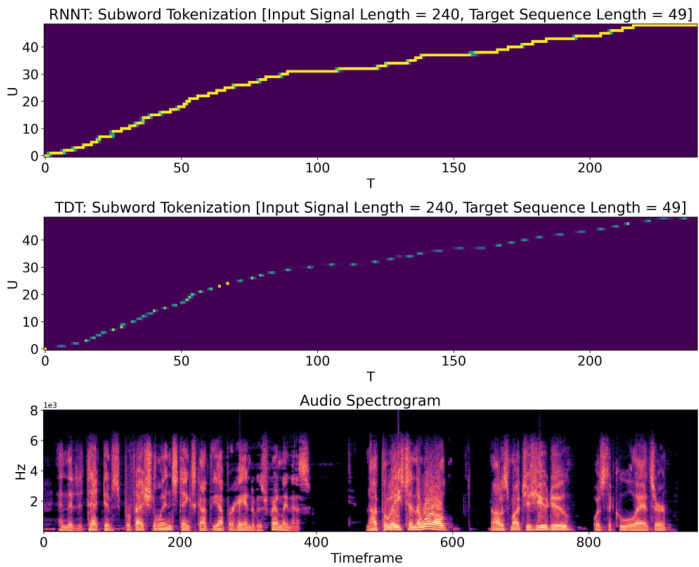
Figure 1. From top to bottom: alignments generated with conventional RNNT, TDT models with config [0-8], and the corresponding spec tr ogram. Each unit in the $T$ axis of the alignment corresponds to 4 frames in the spec tr ogram due to sub sampling. Note, TDT model learns to skip frames. Long skips are not frequently used in the audio where speech is present, but for the 4 relatively silent segments in the audio, where conventional RNNT’s alignment shows mostly horizontal lines, the TDT model uses long durations to skip the majority of frames.

图 1: 从上至下分别为：传统RNNT生成的对齐结果、配置为[0-8]的TDT模型生成的对齐结果，以及对应的频谱图。由于子采样处理，对齐结果中$T$轴的每个单位对应频谱图中的4帧。值得注意的是，TDT模型学会了跳帧机制。在语音活跃的音频段中较少出现长跳帧，但在音频中4段相对静默的片段（传统RNNT对齐结果呈现为水平线）中，TDT模型采用长持续时间跳过了大部分帧。

TDT-based ASR models are more robust to noise than conventional RNN-Ts models, and they don’t suffer from the performance degradation for speech corresponding to the text with repeated tokens.
基于TDT的ASR模型比传统RNN-T模型对噪声更鲁棒，且在文本包含重复token的语音上不会出现性能下降。

Our TDT model implementation will be open-sourced with NVIDIA’s NeMo 1 toolkit.

我们的TDT模型实现将通过NVIDIA的NeMo工具包开源。

2. Background: Transducers

背景：Transducers

An RNN-Transducer 2 (Graves, 2012) consists of an encoder, a decoder (or a prediction network), and a joint network (or a joiner). The encoder and decoder extract higher-level represent at ions of the acoustic and text and feed the output to the joint network, which generates a probability distribution over the vocabulary. The vocabulary includes a special blank symbol $\mathrm{\o}$ ; a text sequence could be augmented by adding an arbitrary number of blanks between any adjacent tokens. During training, we maximize the log-probability $\log P_{\mathrm{RNNT}}(y|x)$ for an audio utterance $x$ with corresponding text $y$ , which requires summing over all possible ways to augment the text sequence to match the audio:

RNN-Transducer 2 (Graves, 2012) 由编码器、解码器 (或称预测网络) 和联合网络 (或称连接器) 组成。编码器与解码器分别提取声学和文本的高阶表征，并将其输出馈送至联合网络，由后者生成词汇表上的概率分布。词汇表包含特殊空白符号 $\mathrm{\o}$，通过在相邻token间插入任意数量空白符可实现文本序列的扩展。训练时，我们通过最大化对数概率 $\log P_{\mathrm{RNNT}}(y|x)$ 来优化音频话语 $x$ 与其对应文本 $y$ 的匹配，这需要穷举所有可能的文本扩展方式来对齐音频：

$$
\begin{array}{l}{{\displaystyle{\mathcal L}{\mathrm{RNNT}}(y|x)=\log P_{\mathrm{RNNT}}(y|x)}}\ {~=\log\sum_{\pi:B^{-1}(\pi)=y}P_{\mathrm{frame-level}}(\pi|x),}\end{array}
$$

where $\pi$ represents an augmented sequence (including $\varnothing$ ), $B(.)$ is the operation to augment a sequence by adding blanks, and $B^{-1}$ is the inverse of the operation $B$ , which removes all the blanks in the sequence.

其中 $\pi$ 表示一个增广序列(包括 $\varnothing$)，$B(.)$ 是通过添加空白来增广序列的操作，而 $B^{-1}$ 是操作 $B$ 的逆运算，它会移除序列中的所有空白。

Computing $P_{\mathrm{RNNT}}(y|x)$ using its definition is intractable since it needs to sum over exponentially many possible augmented sequences. In practice, the probability can be efficiently computed with the forward variables $\alpha(t,u)$ or backward variables $\beta(t,u)$ , which are calculated recursively:

根据其定义计算 $P_{\mathrm{RNNT}}(y|x)$ 是不可行的，因为它需要对指数级数量的可能增广序列求和。实际上，可以通过递归计算前向变量 $\alpha(t,u)$ 或后向变量 $\beta(t,u)$ 来高效求解该概率：

$$
\begin{array}{r l}&{\alpha(t,u)=\alpha(t-1,u)P(\varnothing|t-1,u)}\ &{\phantom{\alpha(t,u)=}+\alpha(t,u-1)P(y_{u}|t,u-1)}\ &{\beta(t,u)=\beta(t+1,u)P(\varnothing|t,u)}\ &{\phantom{\beta(t,u)=}+\beta(t,u+1)P(y_{u+1}|t,u).}\end{array}
$$

with recursion base conditions $\alpha(1,0)=1$ and $\beta(T,U)=$ $P(\emptyset|T,U)$ . In order to make this recursion well-defined, we require that both $\alpha(t,u)$ and $\beta(t,u)$ are zero outside domain $1\leq t\leq T$ and $0\leq u\leq U$ . With those quantities defined, $P_{\mathrm{RNNT}}(y|x)$ could be computed with either the $\alpha$ or $\beta$ efficiently:

递归基条件为 $\alpha(1,0)=1$ 和 $\beta(T,U)=$ $P(\emptyset|T,U)$。为确保递归定义明确，我们要求 $\alpha(t,u)$ 和 $\beta(t,u)$ 在定义域 $1\leq t\leq T$ 和 $0\leq u\leq U$ 之外均为零。定义这些量后，$P_{\mathrm{RNNT}}(y|x)$ 可以通过 $\alpha$ 或 $\beta$ 高效计算：

$$
P_{\mathrm{RNNT}}(y|x)=\alpha(T,U)P(\varnothing|T,U)=\beta(1,0).
$$

Then we could compute the loss function as,

然后我们可以计算损失函数为，

$$
\begin{array}{r}{\mathcal{L}{\mathrm{RNNT}}(y|x)=\log P_{\mathrm{RNNT}}(y|x).}\end{array}
$$

3. Token-and-Duration Transducers

3. Token 与时长传感器

A Token-and-Duration Transducer (TDT) differs from conventional transducers in that it predicts the token duration of the current emission. Namely, the TDT joiner generates two sets of output, one for the output token, and the other for the duration of the token (see Fig. 2). 3 Let us first define a joint probability $P(v,d|t,u)$ as the probability of generating token $v$ ( $v$ could either be a text token or $\mathrm{\o}$ ), with duration $d$ at location $(t,u)$ . We assume that token and durations are conditionally independent:

Token-and-Duration Transducer (TDT) 与传统转换器的区别在于它能预测当前发射的token时长。具体而言，TDT连接器会生成两组输出：一组对应输出token，另一组对应token的时长 (见图2)。3 我们首先定义联合概率 $P(v,d|t,u)$ 为在位置 $(t,u)$ 处生成token $v$ ( $v$ 可以是文本token或 $\mathrm{\o}$ ) 且时长为 $d$ 的概率。假设token与时长是条件独立的：

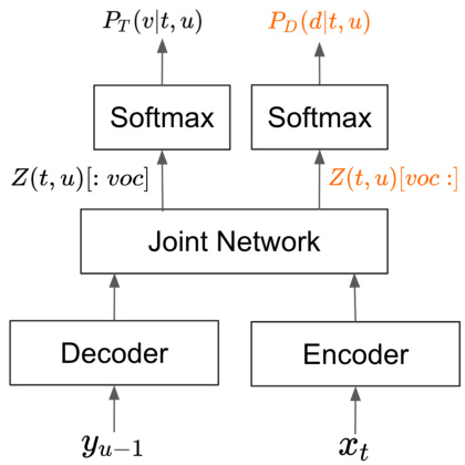
Figure 2. Architecture of a TDT model, which contains an encoder, a decoder, and a joint network. The TDT joint network emits two sets of output, one for the output token $Z(t,u)[:\mathrm{voc}]$ , and the other for the duration of the token $Z(t,u)[\operatorname{voc}[$ . The two distributions are jointly trained during model training.

图 2: TDT模型架构，包含编码器、解码器和联合网络。TDT联合网络输出两组结果：一组用于输出token $Z(t,u)[:\mathrm{voc}]$ ，另一组用于token持续时间 $Z(t,u)[\operatorname{voc}[$ 。这两个分布在模型训练过程中联合训练。

$$
P(v,d|t,u)=P_{T}(v|t,u)P_{D}(d|t,u)
$$

where $P_{T}(.)$ and $P_{D}(.)$ correspond to the token distribution and duration distribution, respectively. Next, we can compute the forward variables $\alpha(t,u)$ :

其中 $P_{T}(.)$ 和 $P_{D}(.)$ 分别对应 token 分布和时长分布。接下来，我们可以计算前向变量 $\alpha(t,u)$：

$$
\begin{array}{r l}{\alpha(t,u)=}&{\displaystyle\sum_{d\in\mathcal{D}\backslash{0}}\alpha(t-d,u)P(\mathcal{D},d|t-d,u)}\ &{\quad\quad+\displaystyle\sum_{d\in\mathcal{D}}\alpha(t-d,u-1)P(y_{u},d|t-d,u-1)}\end{array}
$$

with the same base condition $\alpha(1,0)=1$ as that of the conventional Transducer. Note, this Equation differs from 2 in that, for both non-blank and blank emissions, we need to sum over durations in $\mathcal{D}$ to consider all possible contributions from states that can reach $(t,u)$ , weighted by the corresponding duration probabilities.4 Readers are encouraged to compare those Equations with the transition arcs in Figure 3 to see the connections. The total output probability

在基础条件 $\alpha(1,0)=1$ 与传统Transducer相同的情况下。需要注意的是，该方程与式2的区别在于，对于非空白和空白发射，我们需要在 $\mathcal{D}$ 中对持续时间求和，以考虑所有可能到达状态 $(t,u)$ 的贡献，并按相应的持续时间概率加权。4 建议读者将这些方程与图3中的转移弧进行比较以理解其关联。总输出概率

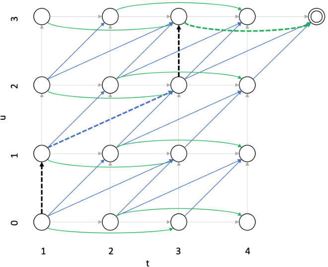
Figure 3. Output probability lattice of TDT model with supported durations $^{{0,1,2}}$ . We follow the convention in (Graves, 2012) making $t$ start with 1 and $u$ with 0. The probability of observing the first $u$ output labels in the first $t$ frames is represented by node $(t,u)$ . Dotted arrows constitute a complete path in the lattice.

图 3: 支持时长 $^{{0,1,2}}$ 的TDT模型输出概率网格。我们遵循 (Graves, 2012) 的惯例，令 $t$ 从1开始，$u$ 从0开始。节点 $(t,u)$ 表示在前 $t$ 帧观测到前 $u$ 个输出标签的概率。虚线箭头构成网格中的完整路径。

$P_{\mathrm{TDT}}(y|x)$ is computed through $\alpha$ at the terminal node: 5

$P_{\mathrm{TDT}}(y|x)$ 通过终端节点的 $\alpha$ 计算得出：5

$$
P_{\mathrm{TDT}}(y|x)=\alpha(T+1,U)
$$

The backward variables $(\beta)$ are computed as,

后向变量 $(\beta)$ 的计算公式为,

$$
\begin{array}{r}{\beta(t,u)=\displaystyle\sum_{d\in\mathcal{D}\backslash{0}}\beta(t+d,u)P(\emptyset,d|t,u)\quad}\ {+\displaystyle\sum_{d\in\mathcal{D}}\beta(t+d,u+1)P(y_{u+1},d|t,u)\quad}\end{array}
$$

with the base condition $\beta(T+1,U)=1$ . The probability of the whole sequence is $P_{\mathrm{TDT}}(y|x)=\beta(1,0)$ .

初始条件为 $\beta(T+1,U)=1$。整个序列的概率为 $P_{\mathrm{TDT}}(y|x)=\beta(1,0)$。

With those quantities defined, we define TDT loss as

在定义这些量的基础上，我们将TDT损失定义为

$$
{\mathcal{L}}{\mathrm{TDT}}=-\log P_{\mathrm{TDT}}(y|x)
$$

3.1. TDT Gradient Computation

3.1. TDT梯度计算

We derive an analytical solution for the gradient of the TDT loss, since automatic differentiation for transducer loss is highly inefficient. 6 The gradient of the TDT loss $\mathcal{L}$ has two parts. The first part is the gradient with respect to the token probabilities $P_{T}(v|t,u)$ :

我们推导了TDT损失的梯度解析解，因为自动微分计算换能器损失效率极低。TDT损失$\mathcal{L}$的梯度包含两部分：第一部分是关于token概率$P_{T}(v|t,u)$的梯度：

$$
\frac{\partial\mathcal{L}{\mathrm{TDT}}}{\partial P_{T}(v|t,u)}=-\frac{\alpha(t,u)b(v,t,u)}{P_{\mathrm{TDT}}(y|x)}
$$

Note, $b(v,t,u)$ can be interpreted as a weighted sum of $\beta$ ’s that are reachable from $(t,u)$ , where the weights are from the duration probabilities.

注意，$b(v,t,u)$ 可以解释为从 $(t,u)$ 可达的 $\beta$ 的加权和，其中权重来自持续时间概率。

The second part is the gradient with respect to the duration probabilities $P_{D}(d|t,u)$ :

第二部分是关于时长概率 $P_{D}(d|t,u)$ 的梯度：

$$
\frac{\partial\mathcal{L}{\mathrm{TDT}}}{\partial P_{D}(d|t,u)}=-\frac{\alpha(t,u)c(d,t,u)}{P(y|x)}
$$

3.2. Gradient with Transducer Function Merging

3.2. 基于Transducer函数融合的梯度

The $P_{T}(v|t,u)$ terms in the Transducer loss are usually computed with a softmax function. Thus the gradients of the TDT loss have to go through the gradient of the softmax function to be passed to the previous layers, which could be costly. We use Transducer function merging proposed in (Li et al., 2019) to directly compute the gradient of the Transducer loss with respect to the pre-softmax logits $(h^{v}(t,u))$ :

Transducer损失中的$P_{T}(v|t,u)$项通常通过softmax函数计算。因此，TDT损失的梯度需经过softmax函数的梯度传递至前层，这一过程可能代价高昂。我们采用(Li et al., 2019)提出的Transducer函数合并方法，直接计算Transducer损失相对于softmax前对数$(h^{v}(t,u))$的梯度：

$$
\frac{\partial\mathcal{L}{\mathrm{TDT}}(y|x)}{\partial h^{v}(t,u)}=\frac{P_{T}(v|t,u)\alpha(t,u)\Big[\beta(t,u)-b(v,t,u)\Big]}{P_{\mathrm{TDT}}(y|x)}
$$

where $b(v,t,u)$ is defined in Eq. 11. Note we apply function merging only to the token logits, not duration logits since the latter usually has very small dimensions, and the negligible efficiency improvements do not outweigh the added complexity in implementation.

其中 $b(v,t,u)$ 由公式 11 定义。请注意，我们仅对 token 逻辑值 (token logits) 应用函数合并，而不对持续时间逻辑值 (duration logits) 应用该操作，因为后者通常具有非常小的维度，且可忽略的效率提升无法抵消实现中增加的复杂性。

3.3. Logits Under-normalization

3.3. Logits 欠归一化

We adopt the logit under-normalization method from $\mathrm{{{Xu}}}$ et al., 2022) during the training of TDT models, in order to encourage longer durations. In our TDT implementations, we compute $P_{T}(v|t,u)$ in the log domain in order to have better numerical stability. The log probabilities $\log P_{T}(v|t,u)$ are computed from the logits $h^{v}(t,u)$ corresponding to token $v$ :

我们在TDT模型训练中采用了$\mathrm{{{Xu}}}$等人(2022)提出的对数欠归一化方法，以鼓励生成长持续时间片段。具体实现时，我们在对数域计算$P_{T}(v|t,u)$以获得更好的数值稳定性。其中对数概率$\log P_{T}(v|t,u)$由token $v$对应的logits $h^{v}(t,u)$计算得出：

$$
\begin{array}{r}{\log P_{T}(v|t,u)=\log\mathrm{{softmax}}_{v^{\prime}}(h^{v^{\prime}}(t,u)).}\end{array}
$$

Algorithm 1 Greedy Inference of Conventional Transducer

算法 1 传统 Transducer 的贪心推理

| | 1: 输入: 声学输入 c |
| | 2: enc = 编码器(c) |
| | 3: hyp =[] |
| 4:t=0 | |
| | 5: while t < len(enc) do |
| 6: | dec = 解码器(hyp) |
| 7: | joined = 联合(enc[t], dec) |
| 8: | idx = argmax(joined) |
| 9: | if token 不为空 then |
| 10: | hyp.append(idx2token[idx]) |
| 11: | else |
| 12: | t+=1 |
| 13: | end if |
| 14:endwhile | |
| | 15: return hyp |

The TDT model uses the pseudo “probability” $P_{T}^{\prime}(v|t,u)$ in its forward and backward computation, which undernormalize the logits in the following way:

TDT模型在其前向和后向计算中使用伪"概率" $P_{T}^{\prime}(v|t,u)$ ，通过以下方式对logits进行欠规范化：

$$
\log P_{T}^{\prime}(v|t,u)=\log\mathrm{{.softmax}}_{v^{\prime}}(h^{v^{\prime}}(t,u))-\sigma.
$$

The under-normalization is only used in training, which encourages TDT models to prioritize emissions of any token (blank or non-blank) with longer durations. The gradients that incorporate the logit under-normalization method are shown in Eq. 17,

训练中仅采用欠归一化方法，以促使TDT模型优先输出持续时间更长的任何token（空白或非空白）。结合对数欠归一化方法的梯度计算如公式17所示，

$$
\frac{\partial\mathcal{L}{\mathrm{TDT}}(y|x)}{\partial h^{v}(t,u)}=\frac{P_{T}(v|t,u)\alpha(t,u)\Big[\beta(t,u)-\frac{b(v,t,u)}{\exp(\sigma)}\Big]}{\exp\Big[\mathcal{L}_{\mathrm{TDT}}(y|x)\Big]}
$$

where $b(v,t,u)$ are defined in Eq. 11.7 Note that Eq. 17 is similar to Eq. 14, with the only difference being for TDT, the b(v, t, u) term is scaled by exp1(σ) .

其中 $b(v,t,u)$ 由式 11.7 定义。注意式 17 与式 14 相似，唯一区别在于 TDT 中 b(v, t, u) 项按 exp1(σ) 进行了缩放。

3.4. TDT Inference

3.4. TDT 推理

We compare the inference algorithms of conventional Transducer models (Algorithm 1) and TDT models (Algorithm 2), which fully utilize the duration output. Note, that for TDT, an additional distribution over durations is computed from the joiner (line 9). This duration can increment $t$ by more than one (line 13), compared with line 12 of conventional Transducer algorithm, where $t$ could only be incremented by 1 at a time, and this only happens for blank emissions. This is the key place that makes TDT inference faster.

我们比较了传统Transducer模型（算法1）和TDT模型（算法2）的推理算法，后者充分利用了时长输出。需要注意的是，TDT模型通过联结器额外计算了时长分布（第9行）。与传统Transducer算法第12行（每次只能将$t$递增1，且仅发生在空白符发射时）相比，此时长可使$t$的递增幅度大于1（第13行）。这正是TDT推理速度更快的关键所在。

4. Experiments

4. 实验

Algorithm 2 Greedy Inference of TDT Models

算法 2 TDT模型的贪婪推断

TDT配置	WER(%)	时间(s)	相对加速
RNNT	2.14	256
0-2	2.35	175	1.46X
0-4	2.17	129	1.98X
0-6	2.14	119	2.15X
0-8	2.11	117	2.19X

We evaluate our model in three different tasks: speech recognition, speech translation, and spoken language understanding. We use the NeMo (Kuchaiev et al., 2019) toolkit for all experiments. Unless specified otherwise, we use ConformerLarge for all tasks. 8 For acoustic feature extraction, we use audio frames of $10\mathrm{ms}$ and window sizes of $25~\mathrm{ms}$ . Our model has a conformer encoder with 17 layers with numheads $=8$ , and relative position embeddings. The hidden dimension of all the conformer layers is set to 512, and for the feed-forward layers in the conformer, an expansion factor of 4 is used. The convolution layers use a kernel size of 31. At the beginning of the encoder, convolution-based subs-ampling is performed with sub sampling rate 4. All models have around 120M parameters, The exact number of parameters may vary, depending on the size of the subword vocabulary and durations used with TDT models. We use different subword-based tokenizers for different models, which will be described in their respective sections. Unless specified otherwise, logit under-normalization is used during training with $\sigma=0.05$ . For all experiments, we train our models for no more than 200 epochs, and run checkpoint-averaging performed on 5 checkpoints with the best performance on validation data, to generate the model for evaluation. We run non-batched greedy search inference 9 for all evaluations reported in this Section. TDT Batched inference is discussed in Section 5.2. No external LM is used in any of our experiments.

我们在三项不同任务中评估模型：语音识别、语音翻译和口语理解。所有实验均使用NeMo (Kuchaiev et al., 2019)工具包。除非另有说明，所有任务均采用ConformerLarge架构。声学特征提取采用$10\mathrm{ms}$音频帧和$25~\mathrm{ms}$窗长。模型配置为17层Conformer编码器，注意力头数$=8$并采用相对位置编码。所有Conformer层的隐藏维度设为512，前馈网络扩展因子为4。卷积层核尺寸为31。编码器起始端采用基于卷积的4倍降采样。模型参数量约1.2亿，具体数值因TDT模型采用的子词词表规模和时长而异。不同模型使用差异化子词分词器，详见各章节说明。训练默认采用$\sigma=0.05$的对数弱归一化。所有实验训练不超过200轮，选取验证集表现最佳的5个检查点进行平均后评估。本节报告结果均采用非批处理贪婪搜索推断，批处理推断详见5.2节。所有实验均未使用外部语言模型。

Table 1. English ASR, Libri speech test-clean. TDT vs RNNT: WER, decoding time, and relative speed-up against the RNNT.

Table 2. English ASR, Libri speech test-other. TDT vs RNNT: WER, decoding time, and relative speed-up against the RNNT.

表 1: 英语ASR (Automatic Speech Recognition)，Libri speech test-clean。TDT与RNNT对比：词错误率(WER)、解码时间及相对于RNNT的加速比。

TDT配置	WER(%)	时间(秒)	相对加速
RNNT	5.11	244
0-2	5.50	171	1.43X
0-4	5.06	128	1.91X
0-6	5.05	118	2.07X
0-8	5.16	115	2.12X

表 2: 英语ASR (Automatic Speech Recognition)，Libri speech test-other。TDT与RNNT对比：词错误率(WER)、解码时间及相对于RNNT的加速比。

4.1. Speech Recognition

4.1. 语音识别

We evaluate TDT for English, German, and Spanish ASR. All ASR models uses Conformer-Large encoder with stateless decoders (Ghodsi et al., 2020), which concatenates the embeddings of the last 2 history words as the decoder output. All models use Byte-Pair Encoding (BPE) (Sennrich et al., 2015) as the text representation with vocabulary size $=1024$ . Fast-emit (Yu et al., 2021) regular iz ation is used in all our models, with $\lambda=0.01$ .

我们对英语、德语和西班牙语的自动语音识别(ASR)进行了TDT评估。所有ASR模型均采用Conformer-Large编码器和无状态解码器(Ghodsi等人，2020)，该架构会将最近两个历史词的嵌入向量拼接作为解码器输出。所有模型均使用字节对编码(BPE)(Sennrich等人，2015)作为文本表示方式，词表大小设为$=1024$。所有模型都采用了快速发射(Fast-emit)(Yu等人，2021)正则化方法，参数设为$\lambda=0.01$。

For each language, the baseline is the conventional Transducer model. We test TDT models with different $\mathcal{D}$ config u rations. We choose consecutive integers as our config u rations, and use a shorthand notation to represent durations from 0 to the maximum value, e.g. $\mathbf{\hat{\Sigma}}^{\omega}0–4\mathbf{\hat{\Sigma}}^{,}$ means $\mathcal{D}={0,1,2,3,4}$ . All models have been trained only on public datasets to make the experiments reproducible.

对于每种语言，基线模型均为传统的Transducer模型。我们测试了不同$\mathcal{D}$配置的TDT模型。选用连续整数作为配置参数，并用简写符号表示从0到最大值的持续时间范围，例如$\mathbf{\hat{\Sigma}}^{\omega}0–4\mathbf{\hat{\Sigma}}^{,}$表示$\mathcal{D}={0,1,2,3,4}$。所有模型仅在公开数据集上训练以确保实验可复现性。

4.1.1. ENGLISH ASR

4.1.1. 英语自动语音识别 (English ASR)

Our English ASR models are trained on the Libri speech (Panayotov et al., 2015) set with 960 hours of speech. Speed perturbation with factors (0.9, 1.0, 1.1) is performed to augment the dataset. TDT models achieve similar accuracy compared to the baseline (RNNT). TDT models are also significantly faster in inference, up to 2.19X and 2.12X with config 0-8 for test-clean and test-other, respectively (see Tables 1 and 2).

我们的英语ASR模型基于960小时的Libri语音数据集(Panayotov et al., 2015)进行训练。采用(0.9, 1.0, 1.1)倍速扰动进行数据增强。TDT模型在准确率上与基线(RNNT)相当，但在推理速度上显著提升：test-clean和test-other测试集在0-8配置下分别达到2.19倍和2.12倍加速(见表1和表2)。

4.1.2. SPANISH ASR

4.1.2. 西班牙语ASR (Automatic Speech Recognition)

Our Spanish models are trained on combination of Mozilla Common Voice (MCV) (Ardila et al., 2019), Multilingual

我们的西班牙语模型训练数据结合了Mozilla Common Voice (MCV) (Ardila et al., 2019) 和多语言

Table 3. Spanish ASR, on CallHome dataset. TDT vs RNNT: WER, decoding time, and relative speed-up against RNNT.

表 3: CallHome数据集上的西班牙语ASR。TDT与RNNT对比：WER、解码时间及相对于RNNT的加速比。

TDT配置	WER(%)	时间(s)	相对加速比
RNNT	19.84	47
0-2	17.95	33	1.42X
0-4	18.57	26	1.81X
0-6	18.06	24	1.96X
0-8	18.73	24	1.96X

Table 4. German ASR on MLS set. TDT vs RNNT: WER, decoding time, and relative speed-up against RNNT.

表 4: MLS数据集上的德语ASR。TDT与RNNT对比：WER、解码时间及相对于RNNT的加速比。

TDT配置	WER(%)	时间(s)	相对加速比
RNNT	3.99	558
0-2	4.10	352	1.59X
0-4	3.93	232	2.41X
0-6	4.00	207	2.70X
0-8	3.95	198	2.82X

Libri speech (MLS) (Pratap et al., 2020), Voxpopuli (Wang et al., 2021a), and Fisher (LDC2010S01) dataset with 1340 hours in total. We evaluate our model on the Spanish Callhome (LDC96S35) test set. We see consistent WER improvement with TDT models compared to RNNT, with up to almost 2 absolute WER points for $0{\cdot}2\mathrm{TDT}$ , and over 1 absolute WER point for our fastest model with configuration $=0{-}8$ (See Table 3). TDT models are much faster than RNNT, with maximum speed up factor of 1.96 for 0-6 and 0-8 TDT configurations.

Libri speech (MLS) (Pratap et al., 2020)、Voxpopuli (Wang et al., 2021a) 和 Fisher (LDC2010S01) 数据集，总计1340小时。我们在西班牙语Callhome (LDC96S35) 测试集上评估模型。与RNNT相比，TDT模型展现出持续的WER提升：$0{\cdot}2\mathrm{TDT}$ 配置下提升近2个绝对WER点，最快模型配置 $=0{-}8$ 时提升超过1个绝对WER点 (参见表3)。TDT模型速度显著快于RNNT，0-6和0-8配置下最高加速比达1.96倍。

4.1.3. GERMAN ASR

4.1.3. 德语ASR (Automatic Speech Recognition)

The German ASR was trained on MCV, MLS, and Voxpopuli datasets, with a total of around 2000 hours. Models are evaluated on MLS test set. TDT models have accuracy similar or better than RNNTs (Table 4). We also observe 2.82X speed up on German MLS test for TDT 0-8 configuration, which is higher than on other datasets.10

德语ASR模型在MCV、MLS和Voxpopuli数据集上进行了训练，总时长约2000小时。模型在MLS测试集上进行评估。TDT模型的准确率与RNNTs相当或更优（表4）。我们还观察到，在德语MLS测试中，TDT 0-8配置实现了2.82倍的加速，这比其他数据集上的表现更高。10

4.2. Speech Translation

4.2. 语音翻译

We evaluate TDT models on English-to-German Speech Translation. For baseline, we directly applies a Conformer Transducer model on speech translation datasets, without any changes to the model. To the best of our knowledge, at the time of writing this paper, there are no reported results with such models, while the closest are from (Xue et al., 2022), where the authors added attention pooling to the joint network in the Transducer model in order to better model reordering in translations. We train our models on a combination of MUST-C V2 (Cattoni et al., 2021), CoVoST V2 (Wang et al., 2021b), ST-TED (Niehues et al., 2018), Europarl-ST (Iranzo-Sanchez et al., 2020), as well as English audio data from Common Voice v6 and VoxPopuli v2 with German text generated with an NMT model trained on WMT21 (Farhad et al., 2021) data. Token iz ation of the text uses the You Token ToMe 11 tokenizer, with a 16k vocabulary size. All models are trained from scratch using the aforementioned training set. Table 5 shows our results on the MUST-C V2 Test dataset. For reference, we also include results of the best publicly available model at the time of writing from (Indurthi et al., 2021).12 Note, the models are not directly comparable with our RNNT and TDT models, since they are trained on different datasets. We see that while baseline RNNT gives a decent result of a BLEU score of 23.21, TDT models consistently improve that with up to 1.26 BLEU score points, and the inference is up to 2.27X faster (see Table 5). TDT models demonstrate a stronger modeling capacity over conventional RNNTs.

我们在英德语音翻译任务上评估TDT模型。基线方案直接使用Conformer Transducer模型处理语音翻译数据集，未对模型结构进行任何修改。据我们所知，截至本文撰写时尚未见此类模型的公开结果，最接近的是(Xue et al., 2022)通过在Transducer模型的联合网络中添加注意力池化来改进翻译中的词序建模。我们的训练数据整合了MUST-C V2 (Cattoni et al., 2021)、CoVoST V2 (Wang et al., 2021b)、ST-TED (Niehues et al., 2018)、Europarl-ST (Iranzo-Sanchez et al., 2020)等数据集，以及来自Common Voice v6和VoxPopuli v2的英文音频数据（其对应德文文本由基于WMT21 (Farhad et al., 2021)训练的NMT模型生成）。文本Token化采用You Token ToMe分词器，词表规模为16k。所有模型均基于上述训练集从头开始训练。

表5展示了我们在MUST-C V2测试集上的结果。作为参照，我们还列出了当前最佳公开模型(Indurthi et al., 2021)的结果。需注意这些模型与我们的RNNT/TDT模型因训练数据差异而不具备直接可比性。实验表明：基线RNNT取得23.21 BLEU分的尚可成绩，而TDT模型能稳定提升最高1.26个BLEU分，推理速度最快提升至2.27倍（见表5）。TDT模型展现出比传统RNNT更强的建模能力。

模型	BLEU (%) 时间(秒)		加速比
(Indurthi et al., 2021)	28.88	N/A	N/A
RNNT	23.21	218
TDT0-2	24.03	143	1.52倍
TDT0-4	24.15	106	2.06倍
TDT 0-8	24.47	96	2.27倍

Table 5. Speech Translation, MUST-C V2 Test dataset. TDT vs RNNT: BLEU score, inference time, and relative inference speedup of different speech translation models.

表 5: 语音翻译，MUST-C V2 测试集。TDT 对比 RNNT：不同语音翻译模型的 BLEU 分数、推理时间及相对推理加速比。

4.3. Spoken Language Understanding

4.3. 口语理解

In this section, we apply TDT models to spoken language understanding (SLU), specifically the Speech Intent Classification and Slot Filling (SICSF) task, which takes audio as input to detect user intents and extract the corresponding lexical fillers for detected entity slots (Bastia nell i et al., 2020). An intent is composed of a scenario type and an action type, while slots and fillers are represented by key-value pairs. The ground-truth intents and slots of input are organized as a Python dictionary, represented as a Python string. The SICSF task is to predict this text based on the input audio. Experiments are conducted using the SLURP (Bastia nell i et al., 2020) dataset, where intent accuracy and SLURP-F1 are used as the evaluation metric.

在本节中，我们将TDT模型应用于口语理解(SLU)任务，具体针对语音意图分类与槽位填充(SICSF)任务。该任务以音频作为输入，检测用户意图并提取对应实体槽位的词法填充物(Bastia nell i et al., 2020)。意图由场景类型和动作类型组成，而槽位及其填充物以键值对形式表示。输入的基准意图与槽位信息以Python字典形式组织，并表示为Python字符串。SICSF任务的目标是根据输入音频预测这段文本。实验采用SLURP数据集(Bastia nell i et al., 2020)，使用意图准确率和SLURP-F1作为评估指标。

Table 6. Speech intent classification and slot filling on SLURP dataset. TDT vs RNNT: Relative speed-up against RNNT.

模型	参数量 (百万)	意图准确率	SLURP F1值	相对加速比
SpeechBrain	96	87.7	76.19	不适用
ESPnet-SLU	109	86.52	76.91	不适用
RNNT	119	88.53	79.41	-
TDT 0-2	119	87.12	79.43	1.17倍
TDT 0-4	119	89.85	80.03	1.17倍
TDT 0-6	119	89.28	80.61	1.28倍
TDT 0-8	119	90.07	79.90	1.28倍

表 6: SLURP数据集上的语音意图分类与槽填充任务性能对比。TDT与RNNT对比：相对RNNT的加速倍数。

Figure 4. Duration distribution during inference on Libri speech test-other. The model is trained with 4X sub sampling. The y-axis shows the number of emissions of different types of durations during the inference of Libri speech test-other datasets.

图 4: Libri speech test-other 推理过程中的时长分布。该模型采用 4 倍子采样训练。y 轴表示在 Libri speech test-other 数据集推理过程中不同类型时长的发射次数。

Our baseline model is a Conformer Transducer model, initialized from our pretrained ASR model 13. We also include results from two state-of-the-art models from ESPNetSLU (Arora et al., 2022) and Speech Brain (Wang et al., 2021c) for comparison. Both ESPNet-SLU and SpeechBrain use HuBERT (Hsu et al., 2021) encoders pretrained on LibriLight-60k (Kahn et al., 2020), while ESPNet-SLU further finetunes the encoder on Libri Speech before training on SLURP. For our TDTs, we use the same duration configurations that contain maximum durations 2, 4, 6, and 8. Different from our ASR and ST experiments that use $\sigma=0.05$ , here we use $\sigma=0.02$ for all experiments since we found using $\sigma=0.05$ may destabilize training for SLURP14.

我们的基线模型是一个Conformer Transducer模型，初始化自我们预训练的ASR模型[13]。为了比较，我们还包含了来自ESPNetSLU (Arora等人，2022)和SpeechBrain (Wang等人，2021c)的两个最先进模型的结果。ESPNet-SLU和SpeechBrain都使用了在LibriLight-60k (Kahn等人，2020)上预训练的HuBERT (Hsu等人，2021)编码器，而ESPNet-SLU在训练SLURP之前进一步在Libri Speech上对编码器进行了微调。对于我们的TDTs，我们使用了相同的持续时间配置，包含最大持续时间2、4、6和8。与使用$\sigma=0.05$的ASR和ST实验不同，这里我们对所有实验使用$\sigma=0.02$，因为我们发现使用$\sigma=0.05$可能会使SLURP14的训练不稳定。

The results are shown in Table 6. While the RNNT baseline already has better performance than ESPNet-SLU and Speech Brain baselines, TDT models with [0-4], [0-6], and [0-8] configurations achieve even better accuracy which makes the new state-of-the-art in the SICSF. In addition, the TDT [0-8] model is $1.28\mathrm{X}$ faster in inference than RNNT.15 The results demonstrate not only the effectiveness but also the efficiency of TDT algorithm applied in SICSF tasks.

结果如表 6 所示。虽然 RNNT 基线模型已经比 ESPNet-SLU 和 Speech Brain 基线表现更好，但采用 [0-4]、[0-6] 和 [0-8] 配置的 TDT 模型实现了更高的准确率，创造了 SICSF 任务的新最优性能。此外，TDT [0-8] 模型的推理速度比 RNNT 快 $1.28\mathrm{X}$。这些结果不仅证明了 TDT 算法在 SICSF 任务中的有效性，还展现了其高效性。

We notice relatively smaller speed-up factors with TDT in this task. This could be explained by the much lower average audio-to-token-length ratio for SICSF tasks. For example, in ASR tasks, the typical ratio between audio length to text length is around 7:1, and the ratio is around 0.89:1 for the

我们注意到在此任务中TDT带来的加速因子相对较小。这可能是由于SICSF任务的平均音频到token长度比低得多所致。例如在ASR任务中，音频长度与文本长度的典型比例约为7:1，而该任务的比例约为0.89:1。

SLURP testset, with average text sequence being longer than audio sequence16. Nevertheless, we see a significant speed up, which also shows that TDT models can bring improvement even for scenarios where the audio sequence is longer than the text sequences.

SLURP测试集，其文本序列平均长度超过音频序列16。尽管如此，我们仍观察到显著的加速效果，这表明TDT模型即使在音频序列长于文本序列的场景下也能带来性能提升。

5. Discussion

5. 讨论

5.1. TDT Emission Analysis

5.1. TDT 排放分析

In this section, we investigate the output distribution of TDT models using Libri speech test-other dataset. First, we collect statistics on the duration predicted during decoding, with different TDT configurations (Fig. 4). For the baseline RNN-T, we treat blank and non-blank symbol emissions as having durations 1 and 0, respectively, since blank advances the $t$ by one and non-blank does not. TDT models with configs [0-2] and [0-4] fully utilize longer durations during inference, with almost all of the durations predicted for the [0-2] model, and around $90%$ of durations for the [0-4] model have the maximum duration. For [0-6] and [0-8] models, the frequencies of predicted long durations are reduced. This is expected since our analysis shows the average ratio of audio length to text length for Libri speech test-other is 5.5:1, smaller than 6. Hence, it is not possible to always emit such long durations.

在本节中，我们使用Libri speech test-other数据集研究TDT模型的输出分布。首先，我们收集了不同TDT配置下解码过程中预测时长的统计信息（图4）。对于基准RNN-T模型，我们将空白(blank)和非空白(non-blank)符号的发射时长分别视为1和0，因为空白会使$t$前进一个单位而非空白不会。采用[0-2]和[0-4]配置的TDT模型在推理过程中充分利用了更长的持续时间——[0-2]模型的预测时长几乎全部达到最大值，而[0-4]模型中约$90%$的预测时长达到最大值。对于[0-6]和[0-8]模型，预测长时长的频率有所降低。这与我们的分析结果一致：Libri speech test-other数据集的音频长度与文本长度平均比值为5.5:1，小于6，因此不可能总是发射如此长的时长。

Next, we collect the frequency of blank emissions vs nonblank emissions (Fig. 5). We can see that as the model incorporates longer durations, fewer and fewer blank emissions are produced with TDT models, while the number of non-blank emissions remains unchanged. TDT models with durations [0-6] and [0-8] have very few blank emissions, indicating that TDT models are close to the theoretical lower bound in terms of the least number of decoding steps.

接下来，我们统计空白发射(blank emissions)与非空白发射(nonblank emissions)的频率(图5)。可以看出，随着模型纳入更长的持续时间，TDT模型产生的空白发射越来越少，而非空白发射的数量保持不变。持续时间[0-6]和[0-8]的TDT模型几乎不产生空白发射，这表明TDT模型在最少解码步数方面已接近理论下限。

Figure 5. Emission counts of blanks VS non-blanks in Libri speech test-other. The model is trained with 4X sub sampling. The y-axis shows the number of emissions of either a blank symbol (red) or a non-blank symbol (blue) during the inference of Libri speech test-other datasets.

图 5: Libri语音测试集(test-other)中空白与非空白符号的发射计数。模型训练采用4倍子采样。y轴表示在Libri语音测试集(test-other)推理过程中空白符号(红色)或非空白符号(蓝色)的发射次数。

5.2. TDT Batched Inference

5.2. TDT 批量推理

Note, the conventional transducer loss $\scriptstyle{\mathcal{L}}{\mathrm{Transducer}}$ is computed on the token logits only, and the duration logits will not take part in the computation nor get updated. We found that the sampled loss solves the aforementioned performance degradation issue. Table 7 shows the ASR performance and inference speed of TDT models when training with $\omega=0.1$ , and running inference with batch ${}_{=4}$ . We even see slightly improved ASR accuracy, as well as inference speed-up with batched inference with TDT. 17

需要注意的是，传统的传感器损失 $\scriptstyle{\mathcal{L}}{\mathrm{Transducer}}$ 仅基于 token 逻辑值计算，持续时间逻辑值不参与计算也不会更新。我们发现采样损失解决了上述性能下降问题。表 7 展示了 TDT 模型在训练时使用 $\omega=0.1$ 并以 batch ${}_{=4}$ 进行推理时的 ASR 性能和推理速度。在使用 TDT 进行批处理推理时，我们甚至观察到 ASR 准确率略有提升，同时推理速度也有所加快。17

TDT配置	干净数据	其他数据	总耗时	相对加速比
RNNT	2.13	5.11	274	—
0-2	2.10	4.94	182	1.51倍
0-4	2.15	5.04	151	1.81倍
0-6	2.10	4.91	146	1.88倍
0-8	2.13	5.03	159	1.79倍

Table 7. Batched inference for TDT ASR models, trained with loss sampling $\omega=0.1$ . WER $(%)$ on Libri speech test-clean and test-other. Batch-size ${=}4$ . When different utterances in the same batch predict different durations, we take the minimum of those predictions and advance all utterances in the batch by that amount.

表 7: 采用损失采样 $\omega=0.1$ 训练的 TDT ASR 模型批量推理结果，展示 LibriSpeech 测试集 test-clean 和 test-other 的 WER $(%)$ 。批处理大小 ${=}4$ 。当同一批次中不同语音片段预测出不同时长时，取预测最小值作为批次统一推进步长。

5.3. TDT Robustness to noise

5.3. TDT 对噪声的鲁棒性

In this section, we compare the noise robustness for TDT and RNNT ASR models. For this, we run inference on Libri speech test-clean augmented with noise in different signal-noise-ratios (SNRs). For each utterance, we ran-domly select a noise sample from MUSAN (Snyder et al., 2015) and Freesound 18. The noise sample is sub-segmented if it’s longer than the utterance, or repeated if it’s shorter than the utterance. The utterance samples are augmented with noise samples in 0, 5, 10, 15, and 20 SNRs. We report the WER and inference time of conventional Transducers and TDT models with configuration 0-8. We found TDT models perform much better in noisy conditions than conventional Transducers, both in terms of accuracy and speed (Fig. 6). While RNN-T and TDT models achieve similar WERs for clean speech, TDT models gradually outperform RNNT as more noise is added. The inference time for TDT is practically the same for all SNRs. More details of those experiments are in Appendix E.

在本节中，我们比较了TDT和RNNT语音识别(ASR)模型的噪声鲁棒性。为此，我们在不同信噪比(SNR)下对添加噪声的LibriSpeech test-clean数据集进行推理测试。对于每条语音，我们从MUSAN (Snyder et al., 2015)和Freesound 18中随机选择噪声样本：若噪声长于语音则截取子片段，若短于语音则循环填充。测试语音分别在0、5、10、15和20 SNR下进行噪声增强。我们对比了传统Transducer与配置0-8的TDT模型的词错误率(WER)和推理时间。实验发现TDT模型在噪声环境下的准确率和速度均显著优于传统Transducer (图6)。虽然RNN-T和TDT在纯净语音上WER相近，但随着噪声增强，TDT逐渐展现出优势。TDT的推理时间在不同SNR下保持稳定。更多实验细节见附录E。

Figure 6. TDT vs RNNT ASR on noisy speech. WER $(%)$ for Libri speech test-clean with noise added at different SNRs. WER on the original test-clean is shown at $\mathrm{SNR}=+\mathrm{inf}$ . While TDT and RNNT achieve similar WER at low noise conditions, TDT is more robust to noise.

图 6: 带噪语音上的 TDT 与 RNNT ASR 对比。展示了不同信噪比 (SNR) 下添加噪声的 Libri speech test-clean 的单词错误率 (WER $(%)$ )。原始 test-clean 的 WER 显示在 $\mathrm{SNR}=+\mathrm{inf}$ 处。虽然在低噪声条件下 TDT 和 RNNT 的 WER 相近，但 TDT 对噪声具有更强的鲁棒性。

Table 8. WERs with different Transducer models on TTS generated dataset with repeated digits.

模型	词错误率(WER%)
RNNT-LSTM	59.95
RNNT-stateless	64.62
TDT [0-2]	12.59
TDT [0-4]	9.35
TDT [0-6]	6.12
TDT [0-8]	5.78

表 8: 不同Transducer模型在TTS生成数字重复数据集上的词错误率

5.4. TDT Robustness with respect to repeated tokens

5.4. 重复Token下的TDT鲁棒性

We notice that RNN-T model performance significantly degrades when the text sequence has repetitions of the same (subword) tokens, for example:

我们注意到，当文本序列中出现相同（子词）token重复时，RNN-T模型性能会显著下降，例如：

We find TDT models are significantly more robust than RNN-Ts for such cases. We use NeMo TTS to generate 100 audios containing random digits repeating 3 - 5 times and run ASR with different models with results in Table 8. We see that while the conventional RNN-Ts achieve very bad word error rates (all of them with error rates more than $50%$ , regardless of the type of decoder used), TDT models are able to achieve significantly lower error rates, and this effect is more prominent for TDT models with longer durations. With TDT models with durations 0-8, we achieve a word error rate of $5.78%$ , which is more than 10X error rate reduction compared to conventional Transducers.

我们发现TDT模型在此类情况下的鲁棒性显著优于RNN-T。利用NeMo TTS生成100段包含随机数字重复3-5次的音频后，使用不同模型进行自动语音识别(ASR)，结果如表 8 所示。传统RNN-T的词错误率表现极差（无论采用何种解码器类型，错误率均超过 $50%$ ），而TDT模型能实现显著更低的错误率，且持续时间更长的TDT模型优势更为突出。采用持续时间0-8的TDT模型时，词错误率可降至 $5.78%$ ，较传统Transducer模型实现了超过10倍的错误率降低。

This set of experiments also shows that TDT models do not suffer from the potential issue of accumulation of errors induced by consecutive duration predictions that might be inaccurate. More details on the analysis of repeated tokens and our experiments can be found in Appendix F.

这组实验还表明，TDT模型不会因连续持续时间预测可能不准确而导致的误差累积问题受到影响。关于重复token的分析及实验的更多细节见附录F。

5.5. TDT Comparison with Multi-blank Transducers

5.5. TDT与多空白转导器的对比

Multi-blank Transducer (MBT) (Xu et al., 2022) introduces big blank symbols that cover multiple input frames. During inference, when a big blank is emitted, the MBT model skips frames according to the duration of the emitted blank symbol. Compared to multi-blank Transducers which skip frames only with certain blank symbols, TDT models allow frame-skipping for both non-blank and blank symbols, which means potentially larger speed-up factors. We compare MBT and TDT in Table 9. We see that while both MBT

多空白符转导器 (Multi-blank Transducer, MBT) (Xu et al., 2022) 引入了覆盖多个输入帧的大空白符。在推理过程中，当大空白符被发射时，MBT模型会根据发射的空白符时长跳过相应帧数。与仅通过特定空白符跳帧的多空白符转导器相比，TDT模型允许非空白符和空白符同时触发跳帧，这意味着潜在更高的加速比。我们在表9中对比了MBT和TDT的性能差异。

模型	最大时长	词错误率 (WER)	时间	相对加速
RNNT		5.11	244	-
MBT	2	5.15	208	1.17倍
TDT	2	5.50	171	1.43倍
MBT	4	5.05	161	1.52倍
TDT	4	5.06	128	1.91倍
MBT	8	5.18	139	1.76倍
TDT	8	5.16	115	2.12倍

Table 9. Inference and accuracy comparison between 3 type of ASR models: RNNT, multi-blank RNNT (MBT), and TDT. Greedy WER $(%)$ and the total decoding time of the Libri speech test-other with batch $=1$ . Relative speed-up is measured against the RNNT. For MBT max-duration ${1=4}$ means MBT model with big-blankduration $=[2,3,4]$ in addition to the conventional blank. For TDT models, max-duration ${}_{=4}$ means model with durations [0,1,2,3,4].

表 9. 三种ASR模型(RNNT、多空白RNNT(MBT)和TDT)的推理与准确率对比：基于Libri speech test-other数据集(批处理量=1)的贪婪WER $(%)$ 及总解码时间。相对加速比以RNNT为基准。对于MBT模型，max-duration ${1=4}$ 表示除常规空白外还包含大空白时长 $=[2,3,4]$ 的MBT模型。对于TDT模型，max-duration ${}_{=4}$ 表示包含时长[0,1,2,3,4]的模型。

and TDT models give comparable WERs, larger inference speedup factors are seen with TDT models when using the same max-duration configs.

TDT模型在相同最大时长配置下能获得更大的推理加速效果，同时保持与基准模型相当的词错误率(WER)。

6. Conclusion

6. 结论

In this paper, we propose Token-and-Duration Transducers, which extend conventional Transducer models by adding explicit duration modeling. We present detailed derivations of the extended forward-backward algorithm used for TDT models, as well as the close-form solutions for TDT model training. We show that TDT models are superior to conventional Transducers across multiple sequence tasks, including speech recognition, speech translation, and spoken language understanding. In all those tasks, we see better or similar performances with TDT models than conventional Transducers, while TDT models run inference significantly faster, with up to 2.82X speed up. TDT is also more noise-robust, and robust to token repetition than conventional RNN-Ts. Our TDT imple ment ation will be open-sourced in NVIDIA’s NeMo https://github.com/NVIDIA/NeMo toolkit.

本文提出Token-and-Duration Transducers (TDT)模型，通过显式时长建模扩展了传统Transducer模型。我们详细推导了TDT模型使用的扩展前向后向算法，并给出TDT模型训练的闭式解。实验表明，在语音识别、语音翻译和口语理解等多序列任务中，TDT模型均优于传统Transducer：在保持相当或更好性能的同时，推理速度显著提升（最高达2.82倍）。相比传统RNN-T，TDT模型还具有更强的抗噪能力和token重复鲁棒性。我们的TDT实现将在NVIDIA NeMo工具包(https://github.com/NVIDIA/NeMo)中开源。

For future work, we will work on other ways to improve the computational efficiency and accuracy of TDT models, as well as algorithms and implementation for efficient beamsearch with TDT models.

未来工作将探索提升TDT模型计算效率和准确性的其他方法，以及基于TDT模型的高效beamsearch算法与实现方案。

[论文翻译]高效序列转导：联合预测Token与持续时间

原文地址：https://arxiv.org/pdf/2304.06795v2