Robust Lane Detection through Self Pre-training with Masked Sequential Auto encoders and Fine-tuning with Customized PolyLoss
基于掩码序列自编码器自预训练和定制化PolyLoss微调的鲁棒车道线检测
Abstract—Lane detection is crucial for vehicle localization which makes it the foundation for automated driving and many intelligent and advanced driving assistant systems. Available vision-based lane detection methods do not make full use of the valuable features and aggregate contextual information, especially the interrelationships between lane lines and other regions of the images in continuous frames. To fill this research gap and upgrade lane detection performance, this paper proposes a pipeline consisting of self pre-training with masked sequential auto encoders and fine-tuning with customized PolyLoss for the end-to-end neural network models using multi-continuous image frames. The masked sequential auto encoders are adopted to pretrain the neural network models with reconstructing the missing pixels from a random masked image as the objective. Then, in the fine-tuning segmentation phase where lane detection segmentation is performed, the continuous image frames are served as the inputs, and the pre-trained model weights are transferred and further updated using the back propagation mechanism with customized PolyLoss calculating the weighted errors between the output lane detection results and the labeled ground truth. Extensive experiment results demonstrate that, with the proposed pipeline, the lane detection model performance on both normal and challenging scenes can be advanced beyond the state-of-theart, delivering the best testing accuracy $(98.38%)$ ), precision (0.937), and F1-measure (0.924) on the normal scene testing set, together with the best overall accuracy $(98.36%)$ and precision (0.844) in the challenging scene test set, while the training time can be substantially shortened.
摘要—车道检测对车辆定位至关重要,是自动驾驶及众多智能高级驾驶辅助系统的基础。现有基于视觉的车道检测方法未能充分利用有价值的特征和聚合上下文信息,特别是连续帧中车道线与图像其他区域的相互关系。为填补这一研究空白并提升检测性能,本文提出一种结合掩码序列自编码器自预训练与定制化PolyLoss微调的端到端神经网络流程,采用多帧连续图像作为输入。通过掩码序列自编码器以随机掩码图像像素重建为目标进行模型预训练,在微调分割阶段将预训练权重迁移至车道检测任务,采用定制化PolyLoss通过反向传播机制计算输出结果与标注真值间的加权误差。大量实验表明,该方案能使模型在常规和复杂场景下的性能均超越现有最优水平:常规场景测试集获得最佳准确率$(98.38%)$、精确率(0.937)和F1值(0.924),复杂场景测试集取得最优整体准确率$(98.36%)$和精确率(0.844),同时大幅缩短训练时间。
Index Terms— Lane Detection, Self Pre-training, Masked Sequential Auto encoders, PolyLoss, Deep Neural Network
索引术语——车道检测 (Lane Detection)、自预训练 (Self Pre-training)、掩码序列自编码器 (Masked Sequential Autoencoders)、PolyLoss、深度神经网络 (Deep Neural Network)
I. INTRODUCTION
I. 引言
L ANE detection is one of the crucial parts of automated d riving and is the foundation of many intelligent and advanced driving assistant systems. However, lane detection has always been a challenging task, for complex and variable realistic road conditions (these scenes are easily disturbed by factors including shadows, degraded road signs, blocking, poor lighting, and bad weather), and the curved and elongated features of lane lines [1].
车道检测 (Lane detection) 是自动驾驶的关键环节之一,也是众多智能高级驾驶辅助系统的基础。然而,由于现实道路环境复杂多变(易受阴影、路面标识退化、遮挡、光照不足及恶劣天气等因素干扰),加之车道线具有弯曲细长的特征 [1],该任务始终面临巨大挑战。
In recent years, many deep learning models have been
近年来,许多深度学习模型已经
Manuscript submitted for review on August $11^{\mathrm{th}}$ , 2022, revised on May $21^{\mathrm{st}}$ 2023, accepted on July $26^{\mathrm{{th}}}$ , 2023. This work was supported by the Applied and Technical Sciences (TTW), a subdomain of the Dutch Institute for Scientific Research (NWO) through the Project Safe and Efficient Operation of Automated and Human-Driven Vehicles in Mixed Traffic (SAMEN) under Contract 17187. (Corresponding author: Yongqi Dong).
稿件于2022年8月11日提交评审,2023年5月21日修订,2023年7月26日被接收。本研究由荷兰科学研究组织(NWO)下属应用与技术科学部(TTW)通过项目"混合交通中自动与人工驾驶车辆的安全高效运行(SAMEN)"资助(合同号17187)。(通讯作者:Yongqi Dong)
proposed for vision-based lane detection [2]. Before the emergence of deep learning, traditional methods mainly utilize traditional computer vision techniques, which rely on manually manipulated operators to extract handcrafted features, including geometry [3], [4], color [5], etc., to do the detection, and then refine the results using a series of fitting methods, such as Hough transform [6] and B-spline fitting [7]. Although some progress had been made, traditional methods are not robust to complex and challenging traffic scenes. In contrast, deep learning based methods can extract more favorable features automatically and achieve superior performance in a variety of complex environments [2]. Generally, deep learning approaches are currently developed from three main perspectives: segmentation-based [1], [8]–[17], anchor-based [18]–[21], and parameter-based [22], [23], among which the most commonly used approach is the segmentation-based method. The performance of segmentation-based methods for lane detection has been continuously improving with various neural network structures developed. Getting rid of dense layers, fully Convolutional Networks (FCNs) [12], [24] employ solely locally connected layers, e.g., convolution, pooling, and upsampling, to enable efficient learning of inputs images with arbitrary sizes, which makes it well-suited for the varying input images of lane detection. Spatial convolutional neural network (SCNN) [8] adopts customized spatial convolutional layers using slice-by-slice convolutions for message passing to capture essential spatial information and correlation for lane detection. UNet-based [1], [9]–[11], [17], [25] neural networks with symmetrical encoder-decoder structures, can extract features at multiple scales, leading to accurately identifying lane markings of different sizes and shapes. Using similar symmetrical encoder-decoder structures, SegNet-based [26]– [28] models employ pooling indices for upsampling, reducing trainable parameters and memory requirements. Generative Adversarial Neural Network (GAN) [29] with embedding loss can preserve label-resembling qualities and improve the outputs' realism and structure preservation, reducing the need for complex post-processing in lane detection.
针对基于视觉的车道检测提出了多种方法 [2]。在深度学习兴起之前,传统方法主要依赖传统计算机视觉技术,通过人工设计的算子提取手工特征(包括几何特征 [3][4]、颜色特征 [5] 等)进行检测,再使用霍夫变换 [6]、B样条拟合 [7] 等拟合方法优化结果。尽管取得了一定进展,但传统方法对复杂交通场景的鲁棒性不足。相比之下,基于深度学习的方法能自动提取更优特征,在各种复杂环境中表现优异 [2]。
当前深度学习方法主要从三个方向展开研究:基于分割的方法 [1][8-17]、基于锚点的方法 [18-21] 以及基于参数的方法 [22][23],其中基于分割的方法应用最为广泛。随着神经网络结构的演进,基于分割的车道检测性能持续提升。全卷积网络 (FCN) [12][24] 摒弃密集连接层,仅采用卷积、池化和上采样等局部连接层,可高效学习任意尺寸的输入图像,非常适合车道检测中多变的输入场景。空间卷积神经网络 (SCNN) [8] 通过逐片卷积的自定义空间卷积层传递信息,捕捉车道检测所需的关键空间信息与相关性。
基于UNet [1][9-11][17][25] 的对称编码器-解码器结构神经网络能提取多尺度特征,精准识别不同尺寸和形状的车道标线。采用类似对称结构的SegNet系列模型 [26-28] 利用池化索引进行上采样,减少了可训练参数和内存需求。嵌入损失的生成对抗网络 (GAN) [29] 能保持标签相似特性,提升输出结果的真实性和结构保持度,从而降低车道检测中复杂后处理的需求。
On the other hand, self-supervised learning has shown in recent studies [30]–[33] that learning a generic feature representation by self-supervision can enable the downstream tasks to achieve highly desirable performance. The basic idea, masking and then reconstructing, is to input a masked set of image patches to the neural network model and then reconstruct the masked patches at the output, allowing the model to learn more valuable features and aggregate contextual information. When it comes to vision-based lane detection, self-supervised learning can provide stronger feature characterization by exploring interrelationships between lane lines and other regions of the images in the continuous frames for the downstream lane detection task. With self-supervised pretraining, it is also possible to accelerate the model convergence in the training phase reducing training time. Meanwhile, with the aggregated contextual information and valuable features by pre-training, the lane detection results can be further advanced.
另一方面,自监督学习在近期研究[30]–[33]中表明,通过自监督方式学习通用特征表示可使下游任务获得优异性能。其核心思想(掩码重建)是将经过掩码处理的图像块输入神经网络模型,随后在输出端重建被掩码区域,促使模型学习更具价值的特征并聚合上下文信息。在基于视觉的车道线检测任务中,自监督学习能通过探索连续帧中车道线与其他图像区域的关联性,为下游检测任务提供更强的特征表征能力。采用自监督预训练还可加速模型训练阶段的收敛速度,缩短训练时长。同时,预训练获得的聚合上下文信息与高价值特征能进一步提升车道检测效果。
In this paper, a self pre-training paradigm is investigated for boosting the lane detection performance of the end-to-end encoder-decoder neural network using multi-continuous image frames. The masked sequential auto encoders are adopted to pretrain the neural network model by reconstructing the missing pixels from a randomly masked image with mean squared error (MSE) as the loss function. The pre-trained model weights are then transferred to the fine-tuning segmentation phase of the per-pixel image segmentation task in which the transferred model weights are further updated using back propagation with a customized PolyLoss calculating the weighted errors between the output lane detection results and the labeled ground truth. With this proposed pipeline, the model performance for lane detection on both normal and challenging scenes is advanced beyond the state-of-the-art results by considerable ratios.
本文研究了一种自预训练范式,通过利用多连续图像帧提升端到端编码器-解码器神经网络的车道检测性能。该方法采用掩码序列自编码器(masked sequential auto encoders)进行预训练,以均方误差(MSE)作为损失函数重构随机掩码图像的缺失像素。预训练模型权重随后迁移至逐像素图像分割任务的微调阶段,该阶段采用定制化PolyLoss计算车道检测输出与标注真值之间的加权误差,通过反向传播进一步更新迁移权重。实验表明,该方案在常规场景和复杂场景下的车道检测性能均以显著优势超越现有最优结果。
The main contributions of this paper are as follows:
本文的主要贡献如下:
- This study proposes a robust lane detection pipeline through self pre-training with masked sequential auto encoders and fine-tuning with customized PolyLoss, and verified its effectiveness by extensive comparison experiments; 2. A customized PolyLoss is developed and adopted to further improve the capability of the neural network model. Without many extra parameter tuning, the customized PolyLoss can bring a significant improvement in the lane detection segmentation task while substantially accelerating model convergence speed and reducing the training time;
- 本研究提出了一种鲁棒的车道检测流程,通过掩码序列自编码器 (masked sequential auto encoders) 进行自预训练,并采用定制化 PolyLoss 进行微调,通过大量对比实验验证了其有效性;
- 开发并采用了一种定制化 PolyLoss,以进一步提升神经网络模型的能力。无需大量额外参数调整,该定制化 PolyLoss 能在车道检测分割任务中带来显著性能提升,同时大幅加速模型收敛速度并减少训练时间;
- The whole pipeline is tested and verified using three deep neural network structures, i.e., U Net Con vL STM [1], S CNN U Net Con vL STM [10], and S CNN U Net Attention [17], with the S CNN U Net Attention based model delivering the best detection results for normal testing scenes, while S CNN U Net Con vL STM model delivering the best detection results for challenging scenes surpassing baseline models.
- 整个流程使用三种深度神经网络结构进行测试验证,即U Net Con vL STM [1]、SCNN U Net Con vL STM [10]和SCNN U Net Attention [17]。其中基于SCNN U Net Attention的模型在常规测试场景中提供了最佳检测结果,而SCNN U Net Con vL STM模型在挑战性场景中的检测效果超越基线模型。
II. PROPOSED METHOD
II. 研究方法
This study proposes a pipeline for lane detection through self pre-training with masked sequential auto encoders and finetuning segmentation with customized PolyLoss. In the first stage, the images are randomly masked as the inputs, and the neural network model is pre-trained with reconstructing the complete images as the objective. In the second stage, the pretrained neural network model weights are transferred to the segmentation neural network model with the same backbone and only the structure of the output layer is adjusted. In this phase, continuous image frames without any masking are served as inputs. The neural network weights are further updated and fine-tuned by minimizing PolyLoss with the back propagation mechanism. In this study, three neural network models, i.e., U Net Con vL STM [1], S CNN U Net Con vL STM [10], and S CNN U Net Attention [17] are tested. In the last stage, post-processing methods, e.g., Density-based spatial clustering of applications with noise (DBSCAN) [34] for clustering the lane types and curve fitting to smooth the detected lines, are proposed to further improve the overall performance of the detection. However, due to time constraints and computational restrictions and following the convention in literature, e.g., [1], [10], [11], post-processing is not specifically explored in this paper. The framework of the proposed pipeline is illustrated in Fig. 1. In the remaining parts of this section, each phase will be introduced in detail.
本研究提出了一种通过掩码序列自编码器进行自预训练,并结合定制化PolyLoss微调分割的车道检测流程。在第一阶段,图像被随机掩码作为输入,神经网络模型以重建完整图像为目标进行预训练。第二阶段将预训练模型权重迁移至具有相同主干网络的分割模型,仅调整输出层结构。此阶段采用连续无掩码图像帧作为输入,通过反向传播机制最小化PolyLoss来进一步更新和微调网络权重。实验中测试了三种神经网络模型:U-Net-ConvLSTM [1]、SCNN-U-Net-ConvLSTM [10]和SCNN-U-Net-Attention [17]。最后阶段提出采用基于噪声的密度空间聚类(DBSCAN) [34]进行车道类型聚类和曲线拟合平滑检测线等后处理方法以提升整体检测性能。但由于时间限制、计算资源约束及遵循文献惯例[1][10][11],本文未对后处理进行深入探讨。该流程框架如图1所示,本节后续将详细阐述各阶段实现。
A. Preliminary and Network Backbone
A. 初步知识与网络主干
This study tests the proposed pipeline with three hybrid neural network models based on the UNet [25] backbone, i.e, U Net Con vL STM [1], S CNN U Net Con vL STM [10], and S CNN U Net Attention [17]. The three models are in similar structures composing three parts, i.e., encoder Convolutional Neural Network (CNN), Convolutional Long Short-Term Memory (ConvLSTM) block or Attention block, and decoder CNN, and they both work in an end-to-end approach.
本研究基于UNet [25]主干网络测试了三种混合神经网络模型:U-Net-ConvLSTM [1]、SCNN-UNet-ConvLSTM [10]和SCNN-UNet-Attention [17]。这三种模型结构相似,均由三部分组成:编码器卷积神经网络(CNN)、卷积长短期记忆(ConvLSTM)模块或注意力模块、解码器CNN,且均采用端到端的工作方式。
Encoder-decoder is a widely used framework in the field of deep learning with various network structures. It is capable of mapping directly from the original input to the desired output in an end-to-end manner and keeping the input and output of the same size. Such a framework has demonstrated good performances in natural language processing tasks, e.g., machine translation, summary extraction, and computer vision tasks, e.g., target detection, scene perception, and image segmentation e.g., [1], [10], [11], [25]. Lane detection as a typical image semantic segmentation or instance segmentation task can surely be tackled with super results under the encoderencoder structure, e.g., [1], [10], [11], [17].
编码器-解码器 (encoder-decoder) 是深度学习领域广泛采用的框架,具有多种网络结构。它能以端到端方式直接从原始输入映射到目标输出,并保持输入输出尺寸一致。该框架在自然语言处理任务(如机器翻译、摘要生成)和计算机视觉任务(如目标检测、场景感知、图像分割 [1], [10], [11], [25])中均表现出色。作为典型的图像语义分割或实例分割任务,车道线检测在编码器-解码器结构下同样能取得优异效果 [1], [10], [11], [17]。
A commonly used base neural network backbone for lane detection (and also other image segmentation task) is the UNet [25], which is an improved FCN. UNet with a symmetric encoder-decoder structure is originally developed to solve the problem of medical image segmentation. In UNet, a block of its encoder contains two convolutional layers, and the feature map is down sampled using pooling layers to reduce the feature map size and increase the number of channels. The decoder, which is symmetric with the encoder, performs de convolution and upsampling operation for feature recovery and data reconstruction. The decoder CNNs have the same size and number of feature maps as in the encoder but are arranged in the opposite direction, and the feature maps are appended in a direct manner. With symmetrical CNN-based encoder-decoder structure, UNet is widely used in various aspects of segmentation tasks, including lane detection, with outstanding performances.
车道检测(以及其他图像分割任务)常用的基础神经网络主干是UNet [25],它是改进版的FCN。UNet最初是为解决医学图像分割问题而开发的,具有对称的编码器-解码器结构。在UNet中,编码器的每个模块包含两个卷积层,通过池化层对特征图进行下采样以减小尺寸并增加通道数。与编码器对称的解码器则执行反卷积和上采样操作,用于特征恢复和数据重建。解码器的CNN与编码器具有相同尺寸和数量的特征图,但排列方向相反,并以直接拼接方式连接特征图。凭借这种基于CNN的对称编码器-解码器结构,UNet在包括车道检测在内的各类分割任务中表现优异,被广泛采用。
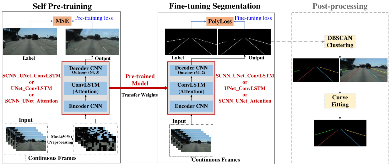
Fig. 1. The framework of the proposed pipeline
图 1: 提出的流程框架
However, the original pure UNet does not consider the slender spatial structure and the correlations and continuity of lane lines in continuous image frames. To tap the temporal continuity of the lane line detection, the ConvLSTM module is embedded between the encoder-decoder in the U Net Con vL STM model [1], which can integrate the time series features extracted from the input multi-continuous frames. To further improve lane detection results, S CNN U Net Con vL STM [10] incorporates SCNN in its single image feature extraction module to make use of the spatial correlations of lane structure and achieves state-of-the-art performance. S CNN U Net Attention [17] which applies a spatial-temporal attention module with liner LSTM in the middle of the encoder and decoder rather than ConvLSTM, can further exploit spatial-temporal correlations and dependencies of different image regions among different frames in the continuous image sequence, and further advance the detection performance. This study implemented and tested U Net Con vL STM, S CNN U Net Con vL STM, and S CNN U Net Attention models to verify the proposed pipeline.
然而,原始的纯UNet未考虑车道线细长的空间结构及其在连续图像帧中的相关性与连续性。为挖掘车道线检测的时间连续性,U Net ConvLSTM模型[1]在编码器-解码器之间嵌入了ConvLSTM模块,可整合从输入的多连续帧中提取的时间序列特征。为进一步提升车道检测效果,SCNN U Net ConvLSTM[10]在其单图像特征提取模块中引入SCNN以利用车道结构的空间相关性,实现了最先进的性能。SCNN U Net Attention[17]则在编码器和解码器中间采用带线性LSTM的时空注意力模块替代ConvLSTM,能更深层次挖掘连续图像序列中不同帧间图像区域的时空关联与依赖关系,从而进一步提升检测性能。本研究实现并测试了U Net ConvLSTM、SCNN U Net ConvLSTM和SCNN U Net Attention模型以验证所提出的流程。
B. Self Pre-training with Masked Sequential Auto encoders
B. 基于掩码序列自编码器的自预训练
For vision-based lane detection, in most of the driving scene image frames, lane lines only account for a small fraction of the whole image, which means there is more spatial redundancy compared to other segmentation tasks. It is vital but challenging to make full use of the valuable features and aggregate contextual information, especially the interrelationships between lane lines and other regions of the images in continuous frames.
基于视觉的车道检测中,在大多数驾驶场景图像帧里,车道线仅占整幅图像的很小部分,这意味着相比其他分割任务存在更多空间冗余。如何充分利用有价值的特征并聚合上下文信息(尤其是连续帧中车道线与图像其他区域的相互关系)至关重要且具有挑战性。
He et al. [31] show that taking advantage of a pre-training strategy by randomly masking a high proportion of input image and reconstructing the original image from the masked patches using the latent representations can improve accuracy and accelerate training speed for downstream tasks. That is, the images with a high masking rate are input into the designed model for reconstruction as a self-supervised learning task, and then the pre-trained model can be migrated to the downstream tasks for fine-tuning. With this pre-training method, the model can gain a better overall "understanding" of the images, since reconstructing the masked pixels in the pre-training phase facilitates the trained model a good generalization capability, which can serve for downstream tasks.
He et al. [31] 研究表明,通过采用随机掩盖高比例输入图像并利用潜在表征从被掩盖区块重建原始图像的预训练策略,可提升下游任务精度并加速训练速度。具体而言,将高掩盖率的图像输入设计模型进行重建作为自监督学习任务,随后将预训练模型迁移至下游任务进行微调。这种预训练方法使模型能获得对图像更全面的"理解",因为在预训练阶段重建被掩盖像素有助于训练模型获得良好的泛化能力,从而服务于下游任务。
Inspired by and upgraded upon the idea of self-training by "random masking-reconstructing" with auto encoders [31], this study proposed to incorporate a pre-training phase with masked sequential auto encoders to pre-train the lane detection models and facilitate their capabilities in aggregating contextual information for feature extraction through continuous frames. In the pre-training phase, $S$ (for the experiments carried out in this study, $S=5$ ) consecutive images are used as the inputs with every image getting certain parts randomly masked. To implement the masking, each of the input images with the size of $(128\times256)$ is firstly divided into non-overlapping patches with the size of $(16\times16)$ , and then random masking is applied to mask a certain ratio of the $(8\times16=128)$ ) patches in each image. The original last image within the input consecutive five image frames is set as the target of the reconstruction task. Using the mean squared error (MSE) as the loss function, the image reconstruction task can be expressed as a minimization problem by (1):
受自编码器通过"随机掩码-重构"进行自训练的思想启发[31],本研究提出引入掩码序列自编码器的预训练阶段,以预训练车道检测模型,并通过连续帧增强其聚合上下文信息进行特征提取的能力。在预训练阶段,使用$S$(本实验取$S=5$)张连续图像作为输入,每张图像随机掩码部分区域。具体实现时,首先将每张尺寸为$(128\times256)$的输入图像划分为$(16\times16)$的非重叠图块,然后随机掩码每张图像中$(8\times16=128)$个图块的一定比例。将连续五帧中的最后一帧原始图像设为重构任务目标,采用均方误差(MSE)作为损失函数,该图像重构任务可表示为式(1)的最小化问题:
$$
\mathrm{min}\qquad\frac{1}{S}{\sum_{k=1}^{S}}d_{2}(M_{k},P_{k})
$$
$$
\mathrm{min}\qquad\frac{1}{S}{\sum_{k=1}^{S}}d_{2}(M_{k},P_{k})
$$
where $S$ is the number of image samples; $M_{k}$ is the pixel value matrix with a size of $(128\times256)$ containing all pixel values in the reconstructed image $k$ reconstructed from the one with masked patches; $P_{k}$ is the pixel value matrix with a size of $(128\times256){,}$ ) containing all pixel values in the original image $k$ ; $d_{2}(\cdot)$ means Euclidean norm which calculates the Euclidean distance between the matrix $M_{k}$ and $P_{k}$ , and can be illustrated by (2):
其中 $S$ 为图像样本数量;$M_{k}$ 是大小为 $(128\times256)$ 的像素值矩阵,包含从掩码块重建的图像 $k$ 中的所有像素值;$P_{k}$ 是大小为 $(128\times256){,}$ 的像素值矩阵,包含原始图像 $k$ 中的所有像素值;$d_{2}(\cdot)$ 表示计算矩阵 $M_{k}$ 与 $P_{k}$ 之间欧氏距离的欧几里得范数,可由式 (2) 表示:
$$
d_{2}(M_{k},P_{k})=\frac{1}{h*w}\sum_{i=1}^{h}\sum_{j=1}^{w}(m_{i,j}-p_{i,j})^{2}
$$
$$
d_{2}(M_{k},P_{k})=\frac{1}{h*w}\sum_{i=1}^{h}\sum_{j=1}^{w}(m_{i,j}-p_{i,j})^{2}
$$
where $m_{i,j}$ and $p_{i,j}$ are the pixel values on $i^{\mathrm{th}}$ row $j^{\mathrm{th}}$ column in the constructed image matrix $M_{k}$ and original image matrix $P_{k}$ respectively; $^h$ is the height of the image with $h=128$ in this study; $w$ is the width of the image with $w=256$ in this study.
其中 $m_{i,j}$ 和 $p_{i,j}$ 分别表示构建图像矩阵 $M_{k}$ 和原始图像矩阵 $P_{k}$ 中第 $i^{\mathrm{th}}$ 行第 $j^{\mathrm{th}}$ 列的像素值;$^h$ 为图像高度 (本研究取 $h=128$);$w$ 为图像宽度 (本研究取 $w=256$)。
Using U Net Con vL STM, S CNN U Net Con vL STM, and S CNN U Net Attention models, the input continuous images with maskings are down sampled four times consecutively by the encoder, and the extracted time-series features of size $(8\times16\times512)$ are then transferred to the ConvLSTM module (or Attention module) for spatial-temporal features integration. Finally, the decoder upsamples the integrated features four times into the same size as the input image and calculates the MSE loss between the reconstructed $5^{\mathrm{th}}$ image and the original $5^{\mathrm{th}}$ image of the input frames. Note in the pre-training phase, the output layers of both U Net Con vL STM, S CNN U Net Con vL STM, and S CNN U Net Attention, are adjusted from the original models reported in [1], [10], and [17], with the number of channels changed to 3 (check Fig. 2).
使用U Net ConvLSTM、SCNN U Net ConvLSTM和SCNN U Net Attention模型时,编码器对带有掩膜的输入连续图像进行四次连续下采样,随后将提取的尺寸为$(8\times16\times512)$的时间序列特征传递至ConvLSTM模块(或Attention模块)进行时空特征整合。最终,解码器对整合后的特征进行四次上采样,使其尺寸与输入图像相同,并计算重建的第$5^{\mathrm{th}}$帧图像与原始输入帧中第$5^{\mathrm{th}}$帧图像之间的均方误差(MSE)损失。需注意的是,在预训练阶段,U Net ConvLSTM、SCNN U Net ConvLSTM和SCNN U Net Attention的输出层均根据[1]、[10]和[17]中报告的原始模型进行了调整,通道数改为3(见图2)。
Regarding the masking ratio, the results of ablation tests with ratios set at $25%$ , $50%$ , or $75%$ found that a $50%$ ratio delivers a balanced performance. Thus, in the pre-training phase, the random masking ratio is set at $50%$ for all models.
关于掩码比例,在分别设置为 $25%$、$50%$ 或 $75%$ 的消融测试中发现,$50%$ 的比例能提供均衡的性能表现。因此,在预训练阶段,所有模型的随机掩码比例均设为 $50%$。
Different from the original masked auto encoders [31] implemented by the vision transformer, the proposed upgrade version of masked sequential auto encoders for pre-training is implemented under the "CNN-ConvLSTM-CNN" or "CNNAttention L STM-CNN" architecture, which can further aggregate valuable image contextual information and spatialtemporal features. By masking the whole continuous 5 image frames and only recovering the last frame, which is also the current frame for lane detection, the proposed upgraded masked sequential auto encoders facilitate the model to learn not only correlations of different regions within one image but also the spatial-temporal interrelationships and dependencies between different regions of the images among continuous frames.
与原始由视觉Transformer实现的掩码自编码器[31]不同,所提出的升级版掩码序列自编码器预训练方案采用"CNN-ConvLSTM-CNN"或"CNN-Attention LSTM-CNN"架构实现,能进一步聚合有价值的图像上下文信息与时空特征。通过掩码连续5帧完整图像并仅恢复最后一帧(即当前车道检测帧),升级版掩码序列自编码器使模型不仅能学习单幅图像内不同区域的关联性,还能掌握连续帧间图像区域的时空交互关系与依赖特性。
C. Fine-tuning with PolyLoss
C. 使用PolyLoss进行微调
Vison-based lane detection as a typical segmentation task aims to classify the image at the pixel level, labeling each pixel with its corresponding class, i.e., lane or background. Generally, for a segmentation task, the input is one image, but in the proposed pipeline, a continuous image sequence is used as input, and only the last image of the continuous sequence is segmented, check Fig 1 for details.
基于视觉的车道检测作为典型的分割任务,旨在像素级别对图像进行分类,将每个像素标记为对应类别(即车道或背景)。通常情况下,分割任务的输入是单张图像,但在本方案中采用连续图像序列作为输入,且仅对连续序列的最后一张图像进行分割,具体细节见图1。
By pre-training with reconstructing the masked patches, the pre-trained model should already get the aggregate contextual information and valuable spatial-temporal features, however, fine-tuning is required to further train the model to adapt it to the per-pixel segmentation task, making full use of those extracted features.
通过预训练重建被遮蔽的补丁,预训练模型应已获得聚合的上下文信息和有价值的时空特征,但仍需微调以进一步训练模型,使其适应逐像素分割任务,充分利用这些提取的特征。
With the elongated structure, lane lines often occupy only a very small fraction of the overall pixels in an image, making lane detection a typical imbalanced two-class segmentation task. Usually, weighted cross entropy loss is adopted for addressing this imbalanced two-class segmentation, which reshapes the standard cross entropy (CE) loss by introducing weighting factors to reduce the weights of the background samples and focus more on the weights of lane pixels. However, literature [35], [36] revealed that weighted CE loss does not perform well under certain situations with severely imbalanced data. To further improve the performance of the lane detection models and improve the capabilities of handling the severe imbalance between lane line and background pixels, this study customizes a PolyLoss (PL for short in the model names), and tests and verifies its effectiveness.
由于车道线具有细长结构,在图像中通常只占极小比例的像素,这使得车道检测成为典型的不平衡二分类分割任务。通常采用加权交叉熵损失(weighted cross entropy loss)来解决这种不平衡问题,该方法通过引入权重因子来降低背景样本的权重,同时增加车道像素的权重,从而重塑标准交叉熵(CE)损失。然而文献[35][36]指出,在数据严重不平衡的特定场景下,加权CE损失表现不佳。为了进一步提升车道检测模型的性能并增强其对车道线与背景像素极端不平衡情况的处理能力,本研究定制了PolyLoss(模型名称中简写为PL),并通过实验验证了其有效性。
PloyLoss is based on the Taylor expansions of CE loss and focal loss (FL), which treats the loss functions as a linear combination of polynomial functions [36]. The CE loss and FL loss can be expressed in (3) and (4):
PolyLoss基于交叉熵损失(CE loss)和焦点损失(focal loss, FL)的泰勒展开式,将损失函数视为多项式函数的线性组合[36]。交叉熵损失和焦点损失可分别表示为式(3)和式(4):
$$
\begin{array}{r l}&{L_{\operatorname{CE}}=-\log(Q_{t})}\ &{L_{\operatorname{FL}}=-\alpha(1-Q_{t})^{\varepsilon}\log(Q_{t})}\end{array}
$$
$$
\begin{array}{r l}&{L_{\operatorname{CE}}=-\log(Q_{t})}\ &{L_{\operatorname{FL}}=-\alpha(1-Q_{t})^{\varepsilon}\log(Q_{t})}\end{array}
$$
where $L_{\mathrm{CE}}$ and $L_{\mathrm{FL}}$ stand for the CE loss and FL loss respectively; $Q_{\imath}$ is the prediction probability of the target ground-truth class; $\alpha,\varepsilon$ are the tunable hyper parameters for $L_{\mathrm{FL}}$
其中 $L_{\mathrm{CE}}$ 和 $L_{\mathrm{FL}}$ 分别代表 CE 损失 (Cross-Entropy loss) 和 FL 损失 (Focal loss);$Q_{\imath}$ 是目标真实类别的预测概率;$\alpha,\varepsilon$ 是 $L_{\mathrm{FL}}$ 的可调超参数。
The loss functions of both CE and $\mathrm{FL}$ can be decomposed into a series of weighted polynomial bases in the form of $\textstyle\sum_{j=1}^{\infty}\alpha_{j}(1-Q_{t})^{j}$ where $j\in\mathbb{Z}^{+}$ , $\alpha_{j}\in R^{+}$ is the polynomial coefficient. Each polynomial basis $(1-Q_{t})^{j}$ is weighted by the corresponding polynomial coefficients $\alpha_{j}\in R^{+}$ , so that it is easy to adjust the different polynomial bases of PolyLoss. The Taylor expansion of FL, indicated by $L_{\mathrm{FL-T}}$ , is given in (5):
CE和$\mathrm{FL}$的损失函数可以分解为一系列加权多项式基的形式$\textstyle\sum_{j=1}^{\infty}\alpha_{j}(1-Q_{t})^{j}$,其中$j\in\mathbb{Z}^{+}$,$\alpha_{j}\in R^{+}$为多项式系数。每个多项式基$(1-Q_{t})^{j}$由对应的多项式系数$\alpha_{j}\in R^{+}$加权,因此可以轻松调整PolyLoss的不同多项式基。FL的泰勒展开式$L_{\mathrm{FL-T}}$如(5)所示:
$$
\begin{array}{l}{{{\cal L}{\mathrm{FL-T}}=-(1-Q_{t})^{\varepsilon}\log(Q_{t})=\displaystyle\sum_{j=1}^{\infty}\frac{(1-Q_{t})^{j+\varepsilon}}{j}}}\ {{{}}}\ {{{\quad\quad=(1-Q_{t})^{1+\varepsilon}+\displaystyle\frac{(1-Q_{t})^{2+\varepsilon}}{2}+\ldots+\displaystyle\frac{(1-Q_{t})^{N+\varepsilon}}{N}+\displaystyle\frac{(1-Q_{t})^{N+1+\varepsilon}}{N+1}+\ldots}}}\end{array}
$$
$$
\begin{array}{l}{{{\cal L}{\mathrm{FL-T}}=-(1-Q_{t})^{\varepsilon}\log(Q_{t})=\displaystyle\sum_{j=1}^{\infty}\frac{(1-Q_{t})^{j+\varepsilon}}{j}}}\ {{{}}}\ {{{\quad\quad=(1-Q_{t})^{1+\varepsilon}+\displaystyle\frac{(1-Q_{t})^{2+\varepsilon}}{2}+\ldots+\displaystyle\frac{(1-Q_{t})^{N+\varepsilon}}{N}+\displaystyle\frac{(1-Q_{t})^{N+1+\varepsilon}}{N+1}+\ldots}}}\end{array}
$$
where $N\in\mathbb{Z}^{+};\varepsilon$ is a modulating factor, with which the FL can simply shift the power $j$ by $\varepsilon$ , i.e., shift all polynomial coefficients horizontally by $\varepsilon$ [36].
其中 $N\in\mathbb{Z}^{+}$;$\varepsilon$ 为调制因子,通过该因子分数阶 (FL) 可将幂次 $j$ 平移 $\varepsilon$,即将所有多项式系数水平平移 $\varepsilon$ [36]。
To improve the model performance and robustness, dropping the higher order polynomials and tuning the leading polynomials are applied in previous studies [36], [37]. Similarly here, after truncating all higher order $\scriptstyle(N+1\to\infty)$ polynomial terms and tuning the leading $N$ polynomials using the perturbation term $\gamma_{j}$ , $j=1,2,3,\cdots,N$ , the truncated $L_{\mathrm{PL-N}}$ is obtained and shown in (6):
为提高模型性能和鲁棒性,先前研究[36]、[37]采用了舍弃高阶多项式并调整主导多项式的方法。类似地,本文在截断所有高阶$\scriptstyle(N+1\to\infty)$多项式项后,通过扰动项$\gamma_{j}$($j=1,2,3,\cdots,N$)调整前$N$项多项式,最终得到截断后的$L_{\mathrm{PL-N}}$如式(6)所示:
$$
\begin{array}{l}{{{\cal L}{\mathrm{PLN}}=(\gamma_{1}+1)(1-Q_{t})^{1+\varepsilon}+(\gamma_{2}+\frac{1}{2})(1-Q_{t})^{2+\varepsilon}+\ldots+(\gamma_{N}+\frac{1}{N})(1-Q_{t})^{N+\varepsilon}}}\ {{\mathrm{}=-(1-Q_{t})^{\varepsilon}\log(Q_{t})+\displaystyle\sum_{j=1}^{N}\gamma_{j}(1-Q_{t})^{j+\varepsilon}}}\end{array}
$$
$$
\begin{array}{l}{{{\cal L}{\mathrm{PLN}}=(\gamma_{1}+1)(1-Q_{t})^{1+\varepsilon}+(\gamma_{2}+\frac{1}{2})(1-Q_{t})^{2+\varepsilon}+\ldots+(\gamma_{N}+\frac{1}{N})(1-Q_{t})^{N+\varepsilon}}}\ {{\mathrm{}=-(1-Q_{t})^{\varepsilon}\log(Q_{t})+\displaystyle\sum_{j=1}^{N}\gamma_{j}(1-Q_{t})^{j+\varepsilon}}}\end{array}
$$
To further simplify the $L_{\mathrm{PL-N}}$ and render it applicable to be easily tuned for different tasks and data sets, Leng et.al [36] carried out extensive experiments and observed that adjusting a single coefficient for the leading polynomial can achieve better performance than the original FL loss. With this, the general form of the finally simplified formula of PolyLoss $L_{\mathrm{{\scriptsize{PL}}}}$ (of FL) is illustrated by (7):
为了进一步简化 $L_{\mathrm{PL-N}}$ 并使其适用于不同任务和数据集的灵活调整,Leng 等人 [36] 进行了大量实验,发现仅调整主导多项式的一个系数即可获得比原始 FL (Focal Loss) 更优的性能。基于此,最终简化的 PolyLoss $L_{\mathrm{{\scriptsize{PL}}}}$ 通用形式如公式 (7) 所示:
$$
L_{\mathrm{pL}}=-\alpha(1-Q_{t})^{\varepsilon}\log(Q_{t})+\gamma(1-Q_{t})^{\varepsilon+1}
$$
$$
L_{\mathrm{pL}}=-\alpha(1-Q_{t})^{\varepsilon}\log(Q_{t})+\gamma(1-Q_{t})^{\varepsilon+1}
$$
where $\alpha,\gamma,\varepsilon$ are the tunable hyper parameters. Adapting it to the imbalanced two-class segmentation task of lane detection, this study further customized (7) into (9) which will be discussed in the following subsection $E$ .
其中 $\alpha,\gamma,\varepsilon$ 是可调超参数。为适应车道检测的不平衡二分类分割任务,本研究进一步将(7)式定制为(9)式,具体讨论见下文 $E$ 小节。
More details about PolyLoss can be referred to in [36].
有关PolyLoss的更多细节可参考[36]。
D. Post processing Phase
D. 后处理阶段
Since in real driving scenarios, it is necessary to identify the types and colors of the lane lines (e.g., dashed lines, continuous double yellow lines), the detected lane lines need to be grouped into different colors to indicate their different types, i.e., lane detection considered as an instance segmentation task. With the fine-tuning lane line segmentation outputs, the DBSCAN [34] algorithm is proposed to cluster the detected lane lines to diffident colors, indicating different types. Then, curve fitting is proposed at the end to smooth the detected lines repairing the discontinuous broken ones (see the post-processing section in Fig. 1). One needs to note that this paper only presents here the idea of post-processing which can serve to upgrade the lane detection results, however, all the results in this paper do not use post-processing which follows the general convention in literature, e.g., [1], [10], [11], [17].
由于在实际驾驶场景中需要识别车道线的类型和颜色(例如虚线、连续双黄线),检测到的车道线需按不同颜色分组以区分其不同类型,即将车道检测视为实例分割任务。基于精细调校的车道线分割输出,本文采用DBSCAN [34]算法对检测到的车道线进行颜色聚类以表征不同类型。最后通过曲线拟合平滑检测线条并修复断裂不连续部分(见图1后处理环节)。需要特别说明的是,本文仅提出可提升车道检测效果的后处理思路,但遵循文献[1][10][11][17]的通用惯例,文中所有实验结果均未使用后处理技术。
E. Implementation Details
E. 实现细节
Configuration Details: In this paper, to reduce the computational payload and save training time, the size of the images for both the training set and test set is set to a resolution of $128\times256$ . In pre-training, the proportion of masked patches is set to $50%$ . Experiments were carried out on two NVIDIA Tesla V100 (32 GB memory) GPUs, using PyTorch version 1.9.0 with CUDA Deep Neural Network library (cuDNN) version 11.1. The batch size is set to be as large as possible, which is 60. The learning rate was initially set to 0.001 with decay applied after each epoch.
配置细节:本文为减少计算负载并节省训练时间,将训练集和测试集的图像尺寸设置为 $128\times256$ 分辨率。在预训练中,掩码块 (masked patches) 的比例设为 $50%$。实验在两块 NVIDIA Tesla V100(32 GB显存)GPU 上完成,使用 PyTorch 1.9.0 版本及 CUDA 深度神经网络库 (cuDNN) 11.1 版本。批次大小 (batch size) 尽可能设为最大值 60,初始学习率为 0.001 并在每轮训练后衰减。
Network Details: In network models of U Net Con vL STM, S CNN U Net Con vL STM, and S CNN U Net Attention, most of the convolutional kernel size is $3\times3$ , except for the SCNN block in S CNN U Net Con vL STM and S CNN U Net Attention. The encoder part (see the left Encoder section in Fig. 2) uses two convolutional layers as a down sampling block, in which the size of the feature map is reduced by half and the number of channels is doubled by the pooling layer. Four successive down sampling blocks are performed, and the last down sampling block does not change the number of output channels compared with its input. The final feature map of the encoder with a size of $8{\times}16{\times}512$ is fed into the spatial-temporal ConvLSTM (or Attention) module.
网络细节:在U Net Con vL STM、SCNN U Net Con vL STM和SCNN U Net Attention的网络模型中,除SCNN U Net Con vL STM和SCNN U Net Attention的SCNN块外,大多数卷积核尺寸为$3\times3$。编码器部分(见图2左侧Encoder部分)使用两个卷积层作为下采样块,其中特征图尺寸通过池化层减半且通道数翻倍。连续执行四个下采样块,最后一个下采样块的输出通道数与其输入保持一致。编码器最终生成尺寸为$8{\times}16{\times}512$的特征图,输入至时空ConvLSTM(或Attention)模块。
The sequential features of the feature map are learned in the ConvLSTM/Attention module, which is equipped with 2 hidden layers of size 512 and outputs an $8{\times}16$ feature map of the same size as its input. The decoder network (check the Decoder part in Fig. 2), is with the same size and number of feature maps as in the encoder but of a reverse-arranged symmetric structure that upsamples the extracted features to the original size of the input image. One needs to note that, in the pre-training task, to recover the image into original RGB pixels, the number of channels in the output layer of the decoder is set as 3; while in the fine-tuning segmentation phase, it is set as 2 for the two-class segmentation task. Therefore, for model weights transfer from the pre-training to fine-tuning phase, the pre-trained model weights are transferred to the fine-tuning model except for the weights of the output layer. Both the pretraining and fine-tuning segmentation phases output images of the same size as the input one. Details can be checked in Fig. 2.
特征图的序列特征在ConvLSTM/Attention模块中学习,该模块配备2个大小为512的隐藏层,并输出一个与输入尺寸相同的$8{\times}16$特征图。解码器网络(见图2中的Decoder部分)具有与编码器相同大小和数量的特征图,但采用反向排列的对称结构,将提取的特征上采样至输入图像的原始尺寸。需要注意的是:在预训练任务中,为将图像恢复至原始RGB像素,解码器输出层的通道数设为3;而在微调分割阶段,针对二分类分割任务则设为2。因此,从预训练到微调阶段的模型权重迁移时,除输出层权重外,预训练模型权重均会迁移至微调模型。预训练和微调分割阶段输出的图像尺寸均与输入一致。具体细节可参见图2。
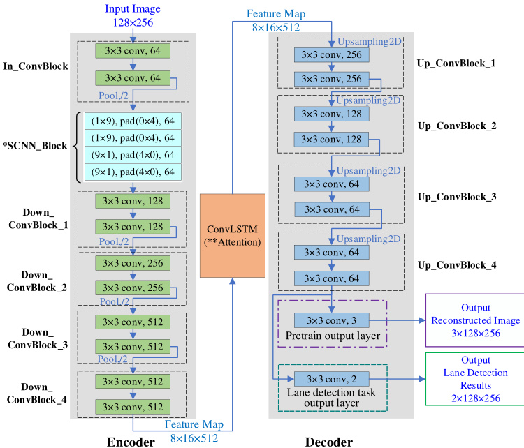
Fig. 2. Pre-training network and lane line detection neural network structure. *SCNN block is for S CNN U Net Con vL STM and S CNN U Net Attention, U Net Con vL STM does not have it. **Attention block is only for S CNN U Net Attention model.
图 2: 预训练网络与车道线检测神经网络结构。*SCNN模块适用于SCNN U Net ConvLSTM和SCNN U Net Attention模型,U Net ConvLSTM不包含该模块。**Attention模块仅适用于SCNN U Net Attention模型。
Loss Function Details: As mentioned before, to make the proposed pipeline work, different loss functions are adopted accordingly in different phases. In the pre-training phase, the objective is to reconstruct the masked images, and for that, the mean square error (MSE) is selected as the loss function.
损失函数细节:如前所述,为了使提出的流程正常工作,不同阶段采用了相应的损失函数。在预训练阶段,目标是重建被遮蔽的图像,为此选择了均方误差 (MSE) 作为损失函数。
While in the fine-tuning segmentation phase, the objective is to segment the pixels into lanes or backgrounds, which is a typical disc rim i native binary segmentation task. This study tested the weighted cross entropy loss and the customized PolyLoss and compared their performances in tackling the imbalanced lane segmentation task. The two tailored losses applied in the fine-tuning segmentation phase are illustrated by (8) and (9).
在微调分割阶段,目标是将像素分割为车道或背景,这是一个典型的圆盘边缘原生二值分割任务。本研究测试了加权交叉熵损失和定制的PolyLoss,并比较了它们在处理不平衡车道分割任务中的性能。微调分割阶段应用的两个定制损失函数如(8)和(9)所示。
$$
\mathrm{CE}=-\frac{1}{T}\sum_{i=1}^{T}[\omega_{1}y_{i}\log(h_{\theta}(x_{i}))+\omega_{0}(1-y_{i})\log(1-h_{\theta}(x_{i}))]
$$
$$
\mathrm{CE}=-\frac{1}{T}\sum_{i=1}^{T}[\omega_{1}y_{i}\log(h_{\theta}(x_{i}))+\omega_{0}(1-y_{i})\log(1-h_{\theta}(x_{i}))]
$$
$$
\operatorname{PL}=-{\frac{1}{T}}\sum_{i=1}^{T}{\left(\alpha{\Biggl[}y_{i}(1-h_{\theta}(x_{i}))^{\varepsilon}\log(h_{\theta}(x_{i}))+{\Biggl]}-\right.}
$$
$$
\operatorname{PL}=-{\frac{1}{T}}\sum_{i=1}^{T}{\left(\alpha{\Biggl[}y_{i}(1-h_{\theta}(x_{i}))^{\varepsilon}\log(h_{\theta}(x_{i}))+{\Biggl]}-\right.}
$$
where $\mathrm{CE}$ and $\mathrm{PL}$ stands for the weighted cross entropy loss and the customized PolyLoss, respectively; $T$ is the number of training examples; $y_{i}$ is the true segmentation label for the training example $i;\omega_{1}$ and $\omega_{\mathrm{0}}$ stands for the weights for lane class and background class respectively; $x_{i}$ is the input training example i; $h_{\theta}(\cdot)$ represents the neural network model with trainable weights $\theta$ ; and $\alpha,\gamma$ , $\varepsilon$ are the tunable hyper parameters for the customized PolyLoss, which are determined by grid search method.
其中 $\mathrm{CE}$ 和 $\mathrm{PL}$ 分别代表加权交叉熵损失和定制化PolyLoss;$T$ 是训练样本数量;$y_{i}$ 是训练样本 $i$ 的真实分割标签;$\omega_{1}$ 和 $\omega_{\mathrm{0}}$ 分别代表车道类和背景类的权重;$x_{i}$ 是输入训练样本 $i$;$h_{\theta}(\cdot)$ 表示具有可训练权重 $\theta$ 的神经网络模型;$\alpha,\gamma$ 和 $\varepsilon$ 是定制化PolyLoss的可调超参数,通过网格搜索方法确定。
Optimizer Details: To efficiently train and validate the proposed model pipeline, different optimizers were tested in different stages. Three optimizers, Stochastic Gradient Descent (SGD), Adaptive Moment Estimation (Adam), and Rectified Adaptive Moment Estimation (RAdam), were tested in the pretraining and fine-tuning segmentation phases. Compared to Adam, SGD requires more parameters, decreases more slowly, and may oscillate continuously on both sides of the gully. Through the tests, Adam performed better than SGD in both the pre-training task and the fine-tuning lane segmentation task. Furthermore, RAdam solves the problem of falling into local optimization that is easily encountered by Adam, and is more robust to the changes of learning rate. Experiments verified that there was even a slight improvement in the model performance of RAdam over Adam. Therefore, the RAdam optimizer was finally chosen for both the pre-training and the fine-tuning segmentation phases.
优化器细节:为高效训练和验证所提出的模型流程,在不同阶段测试了多种优化器。在预训练和微调分割阶段,测试了三种优化器:随机梯度下降 (SGD)、自适应矩估计 (Adam) 和修正自适应矩估计 (RAdam)。与Adam相比,SGD需要更多参数、下降速度更慢,并可能在谷底两侧持续振荡。测试表明,Adam在预训练任务和微调车道分割任务中均优于SGD。此外,RAdam解决了Adam容易陷入局部优化的问题,并对学习率变化具有更强鲁棒性。实验验证RAdam的模型性能相较Adam甚至有轻微提升,因此最终选择RAdam作为预训练和微调分割阶段的优化器。
III. EXPERIMENTS AND RESULTS
III. 实验与结果
A. Datasets Descriptions
A. 数据集描述
To verify the proposed pipeline, a lane image dataset with continuous image frames is required. Although there are various open-sourced lane detection image datasets, e.g., CULane [8], CurveLane [38], seldom do they contain continuous frames. Therefore, this study adopted the tvtLANE [1] dataset, which is upgraded on the TuSimple lane detection challenge dataset, to train and verify the proposed method. There are one integrated training dataset and two testing sets in tvtLANE.
为验证所提出的流程,需要一个包含连续图像帧的车道线数据集。尽管现有多种开源车道检测数据集(如CULane [8]、CurveLane [38]),但大多不包含连续帧。因此本研究采用基于TuSimple车道检测挑战赛数据集升级的tvtLANE [1]数据集进行方法训练与验证。tvtLANE包含一个完整训练集和两个测试集。
The tvtLANE dataset is mainly built based on the TuSimple lane detection challenge dataset. In the original TuSimple dataset, there are 3, 626 training segments and 2, 782 test segments with 20 continuous frames in each segment. The images are collected in different scenes at different times, and only the last frame of each segment, e.g., the $20^{\mathrm{th}}$ frame, is labeled with ground truth. Zou et al. [1] additionally labeled the $13^{\mathrm{th}}$ image in each segment and enlarged the dataset by adding 1, 148 segments of rural driving scenes collected in China. Furthermore, data augmentation methods with cropping, flipping, and rotating operations are employed, and finally a total number 19, 096 continuous segments are produced.
tvtLANE数据集主要基于TuSimple车道检测挑战赛数据集构建。原始TuSimple数据集包含3,626个训练片段和2,782个测试片段,每个片段包含20帧连续图像。这些图像采集自不同时段的不同场景,且仅对每个片段的最后一帧(即第20帧)进行了真实标注。Zou等人[1]额外标注了每个片段的第13帧图像,并通过新增1,148段中国乡村道路驾驶场景片段扩充了数据集规模。此外,研究团队采用裁剪、翻转和旋转等数据增强方法,最终生成了总计19,096个连续片段。
TABLE I SAMPLE METHODS FOR THE TRAINSET AND TESTSET
表 1: 训练集和测试集的采样方法
| 子集 | 标注真值 | 采样步长 | 采样帧 |
|---|---|---|---|
| 训练集 | 第13帧 | 3 | 第1、4、7、10、13帧 |
| 2 | 第5、7、9、11、13帧 | ||
| 1 | 第9、10、11、12、13帧 | ||
| 第20帧 | 3 | 第8、11、14、17、20帧 | |
| 2 | 第12、14、16、18、20帧 | ||
| 1 | 第16、17、18、19、20帧 | ||
| 测试集 #1 正常 | 第13、20帧 | 一 | 第9、10、11、12、13帧 |
| 1 | 第16、17、18、19、20帧 | ||
| 测试集 #2 挑战性 | 全部 | 1 | 第1、2、3、4、5帧 |
| 第2、3、4、5、6帧 | |||
| 第3、4、5、6、7帧 | |||
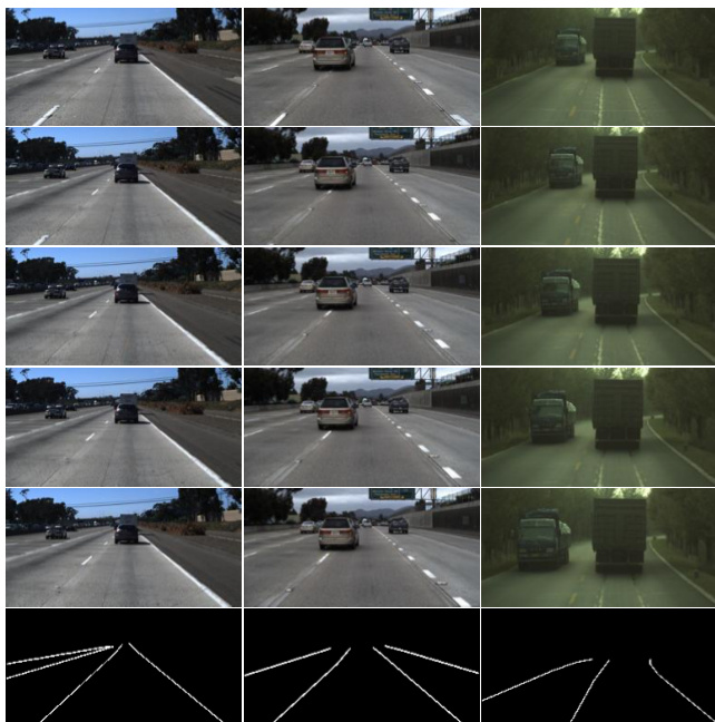
Fig. 3. Image samples in the tvtLANE training set and the test set. The first five images in each column are the inputs of consecutive frames, and the sixth one is the labeled ground truth of the last image in the consecutive frames. The first column is one sample in the training set, the second column is for the test set #1 (normal), and the third column is for test set #2 (challenging).
图 3: tvtLANE 训练集和测试集中的图像样本。每列前五张图像为连续帧输入,第六张为连续帧最后一幅图像的标注真值。第一列为训练集样本,第二列为测试集 #1 (正常场景) ,第三列为测试集 #2 (挑战场景) 。
The tvtLANE consists of two test sets, i.e., test set #1 (normal) which is built on the original TuSimple test set for normal driving scenario testing, and test set #2 (challenging) which consists of 12 challenging driving scenarios for robustness evaluation. More details of tvtLANE can be found in [1], [10].
tvtLANE包含两个测试集:测试集#1(常规)基于原始TuSimple测试集构建,用于常规驾驶场景测试;测试集#2(挑战性)包含12个挑战性驾驶场景,用于鲁棒性评估。更多细节可参阅[1]、[10]。
In this study, 5 images are sampled from the continuous frames with a fixed stride. The sampling strides and frames used in the training and testing sets are elaborated in Table I, and image samples are demonstrated in Fig. 3.
在本研究中,从连续帧中以固定步长采样了5张图像。训练集和测试集中使用的采样步长及帧数详见表1,图像样本示例如图3所示。
B. Evaluation Metrics
B. 评估指标
Overall, the model performance is evaluated in terms of both visual qualitative examination with results demonstration and quantitative analysis with metrics. Considering the visionbased lane detection task as a pixel-level classification task, commonly used metrics, i.e., accuracy, precision, recall, and F1-measure [1], [10], [11], [17], are adopted. The calculations of these metrics are illustrated by (10)-(13).
总体而言,模型性能通过视觉定性展示和定量指标分析两方面进行评估。将基于视觉的车道检测任务视为像素级分类任务时,采用常用指标包括准确率 (accuracy)、精确率 (precision)、召回率 (recall) 和 F1值 (F1-measure) [1][10][11][17],其计算方式如公式(10)-(13)所示。
$$
A c c u r a c y=\frac{T r u l y C l a s s i f i e d P i x e l s}{T o t a l N u m b e r o f P i x e l s}
$$
$$
A c c u r a c y=\frac{T r u l y C l a s s i f i e d P i x e l s}{T o t a l N u m b e r o f P i x e l s}
$$
$$
P r e c i s i o n=\frac{T r u e P o s i t i\nu e}{T r u e P o s i t i\nu e+F a l s e P o s i t i\nu e}
$$
$$
P r e c i s i o n=\frac{T r u e P o s i t i\nu e}{T r u e P o s i t i\nu e+F a l s e P o s i t i\nu e}
$$
$$
R e c a l l=\frac{T r u e P o s i t i\nu e}{T r u e P o s i t i\nu e+F a l s e N e g a t i\nu e}
$$
召回率 = 真阳性 / (真阳性 + 假阴性)
$$
F I-m e a s u r e=2*\frac{P r e c i s i o n*R e c a l l}{P r e c i s i o n+R e c a l l}
$$
$$
F I-m e a s u r e=2*\frac{P r e c i s i o n*R e c a l l}{P r e c i s i o n+R e c a l l}
$$
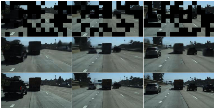
Fig. 4. Visualization of the reconstructing results in the pretraining phase. The first row shows images with $50%$ of the patches masked. The second row shows the reconstructed images after pre-training. The third row shows the original images.
图 4: 预训练阶段重建结果的可视化。第一行展示了被遮挡 50% 图像块 (patches) 的图片。第二行显示了预训练后的重建图像。第三行展示了原始图像。
In the above equations, true positive indicates the number of image pixels that are lane lines and are correctly identified; False positive indicates the number of image pixels that are background but incorrectly classified as lane lines; False negative indicates the number of image pixels that are lane lines but incorrectly classified as background.
在上述等式中,真正例 (true positive) 表示被正确识别为车道线的图像像素数量;假正例 (false positive) 表示实际为背景但被错误分类为车道线的图像像素数量;假负例 (false negative) 表示实际为车道线但被错误分类为背景的图像像素数量。
Furthermore, for estimating the models’ computational complexities, the model parameter size, i.e., Params (M), and the multiply-accumulate (MAC) operations, i.e., MACs (G), are provided.
此外,为估算模型的计算复杂度,提供了模型参数量(即 Params (M))和乘加运算量(即 MACs (G))。
C. Results
C. 结果
In this sub-section, reconstruction performance in the self prtraining phase will be visually demonstrated, while the lane detection testing results of various models on both tvtLANE test set#1 (normal) and tvtLANE test set#2 (challenging) will be evaluated qualitatively and quantitatively.
在本小节中,将直观展示自预训练阶段的重建性能,同时从定性和定量两个维度评估各模型在tvtLANE测试集#1(常规场景)和tvtLANE测试集#2(挑战场景)上的车道线检测效果。
Self pre-training results: Fig. 4 shows the reconstructing results of the masked images in the pr-training phase. It can be seen that the masked patches in the images can be restored very well. Although there are some minor blurs in certain images, the reconstructed images generally recover the main and critical patterns.
自预训练结果:图 4 展示了预训练阶段对掩码图像的重建结果。可以看出,图像中被掩码的区块能够被很好地还原。尽管某些图像存在轻微模糊,但重建后的图像总体上恢复了主要且关键的特征模式。
Testing results on tvtLANE testset#1 (normal): Fig. 5, Fig. 7 (A), and Table. II (a) demonstrate the qualitative and quantitative testing results on tvtLANE testset#1 (normal).
在tvtLANE测试集#1(正常情况)上的测试结果:图5、图7(A)和表II(a)展示了在tvtLANE测试集#1上的定性和定量测试结果。
Qualitatively, for the lane detection segmentation task, the model should be able to accurately predict the total number of lane lines, correctly detecting the location of the lane lines while avoiding unexpected broken lines and blurs. Visualization s of the lane detection results show that models using the proposed self pre-training method generally perform better than those without. Furthermore, models using the customized PolyLoss generally outperform those using weighted cross entropy loss with thinner detected lane lines and fewer blurs. Aligning with previous studies [1], [10], [11], [17], models using multicontinuous image frames defeat those using one single image as indicated in rows (c) and (d) there are fatter lane lines, merged lanes, and blurred areas at the top boundary of the image, and even wrongly detected lane numbers (check the first column in Fig. 7 (A)). One can also notice that even when vehicles or shadings of the vehicles are blocking the lane lines, the models with the proposed pre training method and using the proposed PolyLoss can identify the lane lines completely and continuously with correct locations (check the first, fourth, and sixth columns in Fig. 7 (A)), which is crucial for vehicle localization.
在车道检测分割任务中,该模型应能准确预测车道线总数,正确识别车道线位置,同时避免出现意外的断线和模糊。车道检测结果的可视化显示,采用所提自预训练方法的模型普遍优于未采用该方法的模型。此外,使用定制化PolyLoss的模型相较采用加权交叉熵损失的模型表现更优,检测出的车道线更细且模糊更少。与先前研究[1][10][11][17]一致,如行(c)和(d)所示,使用多连续图像帧的模型优于单帧图像模型——后者会出现车道线变粗、车道合并、图像顶部边界模糊等问题,甚至出现车道数量误判(见图7(A)第一列)。值得注意的是,即使车辆或其阴影遮挡了车道线,采用所提预训练方法并结合PolyLoss的模型仍能完整连续地识别出位置准确的车道线(见图7(A)第一、四、六列),这对车辆定位至关重要。

Fig. 5. Lane detection results obtained by S CNN U Net Attention $\mathrm{PL}^{**}$ on tvtLANE test set #1 (normal) without post-processing.
图 5: 在未进行后处理的情况下,SCNN U-Net Attention $\mathrm{PL}^{**}$ 在tvtLANE测试集#1(正常场景)中获取的车道线检测结果。

Fig. 6 Lane detection results obtained by S CNN U Net Con vL STM PL** on tvtLANE test set #2 (challenging) without post-processing.
图 6: SCNN U-Net ConvLSTM PL**在未进行后处理的情况下,在tvtLANE测试集#2(挑战性场景)中获取的车道检测结果。

Fig. 7 Qualitative visual comparison of the lane detection results testing on tvtLANE test set #1 (normal) (A) and tvtLANE test set #2 (challenging) (B). All results in the figure are without post-processing. (a) Original input images; (b) Ground truth; (c)~(l) are the lane detection results corresponding to the models: (c) SegNet, (d) UNet, (e) Seg Net Con vL STM [1], (f) U Net Con vL STM, (g) U Net Con vL STM CE**, (h) U Net Con vL STM PL**, (i) S CNN Seg Net Con vL STM [10], (j) S CNN U Net Con vL STM, (k) S CNN U Net Con vL STM $\mathrm{CE}^{**}$ , (l) S CNN U Net Con vL STM PL**, (m) S CNN U Net Attention PL**. (Note: CE and PL are short for weighted cross entropy loss and PolyLoss respectively, while ** means the model is pre-trained with the proposed self pre-training method.)
图 7: 在tvtLANE测试集#1(正常)(A)和tvtLANE测试集#2(挑战性)(B)上进行车道检测结果的定性视觉对比。图中所有结果均未经过后处理。(a)原始输入图像;(b)真实标注;(c)~(l)对应各模型的车道检测结果:(c)SegNet,(d)UNet,(e)SegNet ConvLSTM[1],(f)UNet ConvLSTM,(g)UNet ConvLSTM CE**,(h)UNet ConvLSTM PL**,(i)SCNN SegNet ConvLSTM[10],(j)SCNN UNet ConvLSTM,(k)SCNN UNet ConvLSTM $\mathrm{CE}^{**}$,(l)SCNN UNet ConvLSTM PL**,(m)SCNN UNet Attention PL**。(注:CE和PL分别是加权交叉熵损失和PolyLoss的缩写,**表示该模型采用了提出的自预训练方法进行预训练。)
Quantitatively, Table. II (a) demonstrates that the proposed self pre-training method improves the lane detection results for both U Net Con vL STM and S CNN U Net Con vL STM models and the models using the customized PolyLoss all outperform those using the weighted cross entropy loss regarding the accuracy, precision, and F1-measure. To be specific, with the self pre-training pipeline and using the customized PolyLoss, U Net Con vL STM PL** advances a lot from the baseline U Net Con vL STM with testing accuracy improved from $98.00%$ to $98.34%$ , precision improved from 0.857 to 0.921, and F1-measure improved from 0.904 to 0.915; while S CNN U Net Con vL STM PL** also improves a lot from the baseline S CNN U Net Con vL STM with testing accuracy improved from $98.19%$ to $98.38%$ , precision improved from 0.889 to 0.929, and F1-measure improved from 0.918 to 0.922. All the models’ parameter sizes and MACs do not increase.
从量化角度看,表 II (a) 显示所提出的自预训练方法提升了U Net ConvLSTM和SCNN U Net ConvLSTM模型的车道检测效果,且使用定制PolyLoss的模型在准确率、精确率和F1值上均优于使用加权交叉熵损失的模型。具体而言,采用自预训练流程和定制PolyLoss的U Net ConvLSTM PL相比基线U Net ConvLSTM取得显著进步:测试准确率从$98.00%$提升至$98.34%$,精确率从0.857提升至0.921,F1值从0.904提升至0.915;同样地,SCNN U Net ConvLSTM PL相比基线SCNN U Net ConvLSTM也有大幅提升:测试准确率从$98.19%$增至$98.38%$,精确率从0.889增至0.929,F1值从0.918增至0.922。所有模型的参数量与MAC运算量均未增加。
One can find that for both models the most significant improvement was identified in precision, (i.e., 0.857 to 0.921 and 0.889 to 0.929). The higher the precision the lower the false positive is (check (11)) which means the models become more strict on pixel samples to be classified as the lane line contributing to fewer wrong detected lane pixels, which is also illustrated by the thinner detected lane lines in Fig. 7 (A). However, this might increase the number of lane pixels that are incorrectly identified as background, i.e., higher false negative, thus the recall ratio decreases. Therefore, the F1-measure which balances precision and recall, is a more reasonable evaluation measure to serve as the main benchmark [1], [8], [10], [11], [17]. Furthermore, S CNN U Net Attention, which was tested only under the best setting of using pre-training and customized PolyLoss, obtained the best precision (0.937) and F1-measure (0.924) beating all other state-of-the-art baseline models on this tvtLANE testset#1 (normal scene testing).
可以发现,两个模型最显著的提升都体现在精确率上(即从0.857提升至0.921,以及从0.889提升至0.929)。精确率越高,误报率越低(参见(11)),这意味着模型对归类为车道线的像素样本要求更严格,从而减少了错误检测的车道像素,图7(A)中更细的检测车道线也印证了这一点。然而,这可能会增加被误识别为背景的车道像素数量,即更高的漏报率,从而导致召回率下降。因此,平衡精确率与召回率的F1值更适合作为主要评估指标[1][8][10][11][17]。此外,仅在最佳设置(使用预训练和定制化PolyLoss)下测试的SCNN U Net Attention模型,在该tvtLANE测试集#1(正常场景测试)中取得了最佳精确率(0.937)和F1值(0.924),超越了所有其他先进基线模型。
Testing results on tvtLANE test set#2 (challenging): Fig. 6, Fig. 7 (B), and Table II (b) demonstrate the qualitative and quantitative testing results on tvtLANE testset#2 (challenging). Qualitatively, as illustrated in Fig. 6 and Fig. 7 (B), when testing on the challenging driving scenes, all the models do not perform well. However, the results obtained by the models using the proposed self pre-training method are still better than those without pre-training. Especially models adopting the customized PolyLoss still output thinner lanes with less blur and more correct lane numbers.
在tvtLANE测试集#2(挑战性场景)的测试结果:图6、图7(B)和表II(b)展示了tvtLANE测试集#2(挑战性场景)的定性与定量测试结果。定性分析如图6和图7(B)所示,在挑战性驾驶场景测试中,所有模型表现均不理想。但采用本文自预训练方法的模型结果仍优于未预训练模型,尤其采用定制化PolyLoss的模型仍能输出更细、更少模糊且车道数更准确的结果。
Quantitatively, as shown in Table II (b), models with pretraining generally outperform those without regarding the overall accuracy and precision. Typically, using self pretraining method plus the customized PolyLoss, the developed U Net Con vL STM PL** model obtains the best overall accuracy $(98.38%)$ ), and together with other proposed models (with ** in their names), they take all the best accuracies in all 12 challenging scenes; S CNN U Net Con vL STM PL** obtains the best overall precision (0.8444) followed by S CNN U Net Attention $\mathrm{PL}^{**}$ (0.8413), and also together with other proposed models, they fill 11 best precisions out of all the 12 challenging scenes except for only scene 9 blur.
定量分析结果如表 II (b) 所示,在整体准确率和精确率方面,经过预训练的模型普遍优于未预训练的模型。其中,采用自预训练方法结合定制化PolyLoss的U Net Con vL STM PL模型取得了最佳整体准确率$(98.38%)$,同时与其他命名带的模型共同包揽了全部12个挑战场景的最高准确率;SCNN U Net Con vL STM PL*以0.8444的精确率位列榜首,紧随其后的是SCNN U Net Attention $\mathrm{PL}^{**}$ (0.8413),这些模型与其余提案模型共同占据了12个挑战场景中11个场景的最高精确率,仅模糊场景9例外。
TABLE II MODEL PERFORMANCE COMPARISON (a) tvtLANE TEST SET #1 (NORMAL)
表 II: 模型性能对比 (a) tvtLANE 测试集 #1 (正常)
| 模型 | 测试准确率(%) | 精确率 | 召回率 | F1值 | MACs(G) | 参数量(M) |
|---|---|---|---|---|---|---|
| 使用单张图像 | ||||||
| SegNet | 96.93 | 0.796 | 0.962 | 0.871 | 50.2 | 29.4 |
| UNet | 96.54 | 0.790 | 0.985 | 0.877 | 15.5 | 13.4 |
| SCNN* | 96.79 | 0.654 | 0.808 | 0.722 | 77.7 | 19.2 |
| 使用连续多张图像 | ||||||
| LaneNet | 97.94 | 0.875 | 0.927 | 0.901 | 44.5 | 19.7 |
| SegNet_ConvLSTM | 97.92 | 0.874 | 0.931 | 0.901 | 217.0 | 67.2 |
| UNet_ConvLSTM | 98.00 | 0.857 | 0.958 | 0.904 | 69.0 | 51.1 |
| UNet_ConvLSTM_CE** | 98.19 | 0.882 | 0.940 | 0.910 | 69.0 | 51.1 |
| UNet_ConvLSTM_PL** | 98.34 | 0.921 | 0.909 | 0.915 | 69.0 | 51.1 |
| SCNN_SegNet_ConvLSTM | 98.07 | 0.893 | 0.928 | 0.910 | 223.0 | 67.3 |
| SCNN_UNet_ConvLSTM | 98.19 | 0.889 | 0.950 | 0.918 | 93.0 | 51.3 |
| SCNN_UNet_ConvLSTM_CE* | 98.20 | 0.891 | 0.952 | 0.921 | 93.0 | 51.3 |
| SCNN_UNet_ConvLSTM_PL* | 98.38 | 0.929 | 0.915 | 0.922 | 93.0 | 51.3 |
| SCNN_UNet_Attention_PL** | 98.36 | 0.937 | 0.911 | 0.924 | 68.9 | 13.7 |
(b) tvtLANE TEST SET #2 (CHALLENGING)
* Results reported in [11]. ** Results of the models with the proposed self pre-training. $"C E"$ is short for weighted cross entropy loss, and "PL" is short for PolyLoss. Therefore, "U Net Con vL STM $C E^{**\prime\prime}$ means U Net Con vL STM model with self pre-training and using weighted cross entropy loss in the finetuning phase. This naming rule applies to all other models.
(b) tvtLANE 测试集 #2 (挑战场景)
| 挑战场景模型 | overallcurve&o|shadow-3-bright | 1- cclude | 2- bright | 4- occlude | 5- curve | 6-dirty& occlude | 7- urban | 8-blur& curve | 9- blur | 10- shadow | 11- tunnel | 12- dim& occlude |
|---|---|---|---|---|---|---|---|---|---|---|---|---|
| 精度(PRECISION) | ||||||||||||
| SegNet | 0.6080 | 0.6810 | 0.7067 | 0.5987 | 0.5132 | 0.7738 | 0.2431 | 0.3195 | 0.6642 | 0.7091 | 0.7499 | 0.6225 |
| UNet | 0.6754 | 0.7018 | 0.7441 | 0.6717 | 0.6517 | 0.7443 | 0.3994 | 0.4422 | 0.7612 | 0.8523 | 0.7881 | 0.7009 |
| SegNet_ConvLSTM | 0.7563 | 0.8176 | 0.8020 | 0.7200 | 0.6688 | 0.8645 | 0.5724 | 0.4861 | 0.7988 | 0.8378 | 0.8832 | 0.7733 |
| UNet_ConvLSTM | 0.7784 | 0.7591 | 0.8292 | 0.7971 | 0.6509 | 0.8845 | 0.4513 | 0.5148 | 0.8290 | 0.9484 | 0.9358 | 0.7926 |
| UNet_ConvLSTM_CE** | 0.7932 | 0.8004 | 0.8312 | 0.8285 | 0.7661 | 0.8557 | 0.5242 | 0.5567 | 0.7545 | 0.9200 | 0.9312 | 0.8496 |
| UNet_ConvLSTM_PL** | 0.8331 | 0.8429 | 0.8824 | 0.8691 | 0.8125 | 0.9578 | 0.5970 | 0.5591 | 0.8289 | 0.9247 | 0.9634 | 0.7688 |
| SCNN_SegNet_ConvLSTM | 0.7673 | 0.8326 | 0.7497 | 0.7470 | 0.7369 | 0.8647 | 0.6196 | 0.4333 | 0.7371 | 0.8566 | 0.9125 | 0.8153 |
| SCNN_UNet_ConvLSTM | 0.7784 | 0.8182 | 0.8362 | 0.8189 | 0.7359 | 0.8365 | 0.5872 | 0.5377 | 0.8046 | 0.8770 | 0.8722 | 0.7952 |
| SCNN_UNet_ConvLSTM_CE* | 0.8001 | 0.8754 | 0.8672 | 0.8519 | 0.7763 | 0.8664 | 0.5523 | 0.5261 | 0.7396 | 0.8865 | 0.8974 | 0.8115 |
| SCNN_UNet_ConvLSTM_PL** | 0.8444 | 0.9074 | 0.8757 | 0.8644 | 0.8464 | 0.9049 | 0.7177 | 0.4827 | 0.8157 | 0.9440 | 0.9606 | 0.8736 |
| SCNN_UNet_Attention_PL** | 0.8413 | 0.9189 | 0.8763 | 0.8838 | 0.8598 | 0.9238 | 0.6210 | 0.5229 | 0.8847 | 0.9039 | 0.9229 | 0.8408 |
| F1值(F1-MEASURE) | | | | | | | | | | | | |
| SegNet | 0.6727 | 0.8042 | 0.7900 | 0.7023 | 0.6127 | 0.8639 | 0.2110 | 0.4267 | 0.7396 | 0.7286 | 0.7675 | 0.6935 | 0.5822 |
| UNet | 0.6985 | 0.8200 | 0.8408 | 0.7946 | 0.7337 | 0.7827 | 0.3698 | 0.5658 | 0.8147 | 0.7715 | 0.6619 | 0.5740 | 0.4646 |
| SegNet_ConvLSTM | 0.7609 | 0.8852 | 0.8544 | 0.7688 | 0.6878 | 0.9069 | 0.4128 | 0.5317 | 0.7873 | 0.7575 | 0.8503 | 0.7865 | 0.7947 |
| UNet_ConvLSTM | 0.7143 | 0.8465 | 0.8891 | 0.8411 | 0.7245 | 0.8662 | 0.2417 | 0.5682 | 0.8323 | 0.7852 | 0.6404 | 0.4741 | 0.5718 |
| UNet_ConvLSTM_CE** | 0.6537 | 0.8365 | 0.8697 | 0.8263 | 0.7614 | 0.8165 | 0.2440 | 0.5359 | 0.7618 | 0.7206 | 0.4832 | 0.3274 | 0.2595 |
| UNet_ConvLSTM_PL** | 0.6284 | 0.8220 | 0.8731 | 0.8300 | 0.7705 | 0.8295 | 0.1845 | 0.4426 | 0.7278 | 0.5712 | 0.4157 | 0.3545 | 0.4821 |
| SCNN_SegNet_ConvLSTM | 0.7666 | 0.8956 | 0.8237 | 0.7909 | 0.7468 | 0.9108 | 0.4398 | 0.4858 | 0.7379 | 0.7546 | 0.8729 | 0.7963 | 0.8074 |
| SCNN_UNet_ConvLSTM | 0.7024 | 0.8670 | 0.8866 | 0.8405 | 0.7565 | 0.7955 | 0.4179 | 0.5933 | 0.7880 | 0.7285 | 0.6296 | 0.4747 | 0.4134 |
| SCNN_UNet_ConvLSTM_CE* | 0.7327 | 0.8937 | 0.8690 | 0.8426 | 0.7656 | 0.8352 | 0.2493 | 0.5751 | 0.7756 | 0.7122 | 0.7661 | 0.6989 | 0.5420 |
| SCNN_UNet_ConvLSTM_PL** | 0.6711 | 0.8685 | 0.8796 | 0.8161 | 0.7988 | 0.7897 | 0.2853 | 0.4921 | 0.8258 | 0.7255 | 0.5244 | 0.3963 | 0.3255 |
| SCNN_UNet_Attention_PL** | 0.6772 | 0.8530 | 0.8771 | 0.8111 | 0.7579 | 0.7881 | 0.2926 | 0.5057 | 0.8595 | 0.7569 | 0.5857 | 0.3737 | 0.4565 |
| 准确率(ACCURACY %) ** | | | | | | | | | | | | |
| SegNet | 96.57 | 96.72 | 96.16 | 96.01 | 96.83 | 96.50 | 95.93 | 96.16 | 96.39 | 96.12 | 97.26 | 96.79 | 97.37 |
| UNet | 96.68 | 96.68 | 96.00 | 95.78 | 97.06 | 96.35 | 95.45 | 96.35 | 96.58 | 96.62 | 97.50 | 97.53 | 97.58 |
| SegNet_ConvLSTM | 97.83 | 98.10 | 97.38 | 97.52 | 98.17 | 97.72 | 96.98 | 97.92 | 97.61 | 97.08 | 98.39 | 98.07 | 98.26 |
| UNet_ConvLSTM | 97.93 | 97.83 | 97.48 | 97.70 | 97.94 | 97.73 | 97.27 | 97.86 | 97.75 | 97.65 | 98.49 | 98.37 | 98.38 |
| UNet_ConvLSTM_CE | 98.13 | 98.19 | 97.72 | 98.04 | 98.47 | 97.77 | 97.41 | 98.30 | 97.67 | 97.69 | 98.58 | 98.54 | 98.57 |
| UNet_ConvLSTM_PL** | 98.38 | 98.60 | 98.06 | 98.33 | 98.75 | 98.35 | 97.66 | 98.61 | 98.09 | 97.77 | 98.63 | 98.63 | 98.63 |
| SCNN_SegNet_ConvLSTM | 97.90 | 97.95 | 98.08 | 97.21 | 97.68 | 98.39 | 97.73 | 97.11 | 97.80 | 97.48 | 97.29 | 98.50 | - |
- 结果来自文献[11]
** 采用自预训练策略的模型结果
$"CE"$ 表示加权交叉熵损失, "PL" 表示PolyLoss。因此 "UNet_ConvLSTM_CE**" 表示采用自预训练并在微调阶段使用加权交叉熵损失的UNet_ConvLSTM模型。此命名规则适用于所有其他模型。
It is worth noting that the models using the proposed self pretraining deliver slightly worse F1-measures compared to those without pre-training. This is because the models are more strict with the pixels classified as the lane lines which might increase the number of lane pixels that are incorrectly identified as background, i.e., resulting in higher false negatives, thus the recall ratio decreases and the F1-measures get slightly worse (even if there are increases in precisions). From Fig. 7 (B), it is more intuitive to see that the developed models with the proposed pre-training and PolyLoss still show acceptable results better than the baselines.
值得注意的是,采用本文提出的自预训练方案的模型在F1分数上略逊于未预训练的模型。这是因为模型对分类为车道线的像素判定更为严格,可能导致更多车道像素被误识别为背景(即假阴性增加),从而降低召回率,致使F1分数轻微下滑(即使精确度有所提升)。从图7(B)可以更直观地看出,采用所提预训练方案和PolyLoss的模型仍展现出优于基线的可接受结果。
D. Ablation Study and Discussion
D. 消融研究与讨论
Masking ratio: Experimental results in the previous study [32] showed that the masking ratio needs to correspond to the mask patch, i.e., “for a small mask patch size of 8, the masking ratio needs to be as high as $80%$ to perform well”, while “for a large masking patch size of 32, the approach can achieve competitive performance in a wide range of masking ratios $(10%-70%)^{\prime\prime}$ . In this study, the patch size is set as 16, i.e., $(16\times16)$ , and the experimental comparisons were carried out with ratios set as $25%$ , $50%$ , and $75%$ .
掩码比例:先前研究[32]的实验结果表明,掩码比例需与掩码块尺寸相匹配,即"当采用较小的8×8掩码块时,掩码比例需高达80%才能获得良好性能",而"对于32×32的大尺寸掩码块,该方法在较宽的掩码比例范围(10%-70%)内都能保持竞争力"。本研究将块尺寸设定为16×16,并分别采用25%、50%和75%三种比例进行实验对比。
Testing on S CNN U Net Con vL STM model, Fig. 8 (a) shows the average normalized reconstruction loss indicated by mean square error (MSE) of the image reconstruction task during the pre-training phase. It is observed that using a smaller masking ratio leads to lower reconstruction loss, which is easy to understand, as a smaller masking ratio means fewer pixels need to be reconstructed.
在SCNN U Net ConvLSTM模型上的测试中,图8(a)展示了预训练阶段图像重建任务的平均归一化重建损失(以均方误差(MSE)表示)。可以观察到,使用较小的掩蔽比例会导致较低的重建损失,这很容易理解,因为较小的掩蔽比例意味着需要重建的像素更少。
Fig. 8 (b) shows the lane detection performance on the normal driving scene dataset regarding F1-measure with different masking ratios and TABLE III shows the detailed quantitative results.
图 8 (b) 展示了不同遮挡比例下正常驾驶场景数据集的 F1-measure 车道检测性能,表 III 展示了详细的定量结果。
It is found that although the result of masking at a $75%$ ratio achieves the best F1-measure of 0.926 on the normal dataset, it does not perform particularly well on the challenge dataset, where it only achieves an F1-measure of 0.71815 worse than that of masking at a $50%$ ratio (F1-measure at 0.7327).
研究发现,虽然在正常数据集上以75%比例进行掩码 (masking) 的结果达到了最佳F1值0.926,但在挑战数据集上表现欠佳,其F1值仅为0.71815,低于50%掩码比例的结果 (F1值0.7327)。
Furthermore, referring to the results of the pre-training phase, it is clear that masking at a $50%$ ratio delivers balanced results during both the pre-training phase and fine-tuning testing phases. It is more reasonable to adopt the balanced setting to verify the proposed lane detection pipeline and method, and thus, $50%$ was chosen as the masking ratio for all testing models.
此外,参考预训练阶段的结果,显然在预训练阶段和微调测试阶段中,50%的遮蔽比例都能带来平衡的结果。采用这一平衡设定来验证所提出的车道检测流程和方法更为合理,因此所有测试模型均选择50%作为遮蔽比例。
Loss function: Earlier mentioned in this paper, two loss functions (i.e., weighted cross entropy loss and PolyLoss) were tested in the experiments under the proposed pipeline in the fine-tuning segmentation phase. The quantitative comparison results are shown in Table II, and the qualitative results are intuitively demonstrated with visualization s in Fig. 7.
损失函数:前文提到,在微调分割阶段的实验流程中测试了两种损失函数(即加权交叉熵损失和PolyLoss)。定量对比结果如表II所示,定性结果通过图7的可视化效果直观展示。
As shown in Table II (a), testing on tvtLANE test set#1 (normal scene), for both S CNN U Net Con vL STM and
如表 II (a) 所示,在 tvtLANE 测试集#1 (正常场景) 上进行测试时,对于 S CNN U Net Con vL STM 和

Fig 8. Model performance comparison with different masking ratio settings: reconstruction loss in pre-training phase (a), and the F1-measure testing on tvtLANE test set #1 (b)
图 8. 不同掩码比例设置下的模型性能对比:(a) 预训练阶段的重建损失,(b) 在 tvtLANE 测试集 #1 上测试的 F1 值
U Net Con vL STM based models, the overall performance of using PolyLoss outperforms that of weighted cross entropy loss. To be specific, compared with U Net Con vL STM CE**, the U Net Con vL STM PL** model obtains an increase of $0.15%$ in accuracy; a significant increase of 0.039, i.e., around $4.4%$ improvement, in precision; while a bit decrease in recall; and, overall, a better F1-Measure of 0.915 over 0.910. S CNN U Net Con vL STM PL** gets the same superiority patterns over S CNN U Net Con vL STM CE**, and S CNN U Net Con vL STM PL** obtains the second-best F1- measure (0.922), the second-best precision (0.929), and the best accuracy $(98.38%)$ , among all tested models. S CNN U Net Attention $\mathrm{PL}^{**}$ slightly beats S CNN U Net Con vL STM PL in F1-Mesure (0.924) and precision (0.937). The superiority of the customized PolyLoss over weighted cross entropy loss can be explained by that the PolyLoss function is designed as a linear combination of polynomial functions so that the importance of polynomial bases can be adjusted according to the imbalanced dataset and regarding the segmentation task. With the fine-tuned hyper parameters $\alpha,\gamma,\varepsilon$ in (9), the customized PolyLoss is perfectly adjusted to the dedicated lane detection task.
基于U Net Con vL STM的模型中,采用PolyLoss的整体性能优于加权交叉熵损失。具体而言,与U Net Con vL STM CE相比,U Net Con vL STM PL模型的准确率提升了0.15%;精确度显著提高0.039(约4.4%);召回率略有下降;总体F1值从0.910提升至0.915。SCNN U Net Con vL STM PL相较SCNN U Net Con vL STM CE展现出相同优势模式,其F1值(0.922)和精确度(0.929)在所有测试模型中位列第二,准确率(98.38%)则达到最高。SCNN U Net Attention PL**在F1值(0.924)和精确度(0.937)上略胜SCNN U Net Con vL STM PL。这种定制化PolyLoss的优势源于其函数设计:通过多项式基的线性组合,可根据数据不平衡程度和分割任务需求调整各多项式权重。配合公式(9)中调优的超参数α、γ、ε,该损失函数能完美适配车道检测任务。
The model using PolyLoss also performs better than the ones using weighted cross entropy loss in almost all challenging scenes regarding accuracy and precision. In particular, testing on the challenging driving scenes dataset, U Net Con vL STM $\mathrm{PL}^{**}$ gets the highest overall accuracy at $98.38%$ , while S CNN U Net Con vL STM PL** obtains the best overall precision at 0.8444.
使用PolyLoss的模型在几乎所有具有挑战性的场景中,其准确率和精确度均优于采用加权交叉熵损失的模型。特别是在挑战性驾驶场景数据集上的测试中,U Net Con vL STM 以 $98.38%$ 的总准确率位居榜首,而SCNN U Net Con vL STM PL**则以0.8444的总精确度表现最佳。
Training time and model complexity: In addition to the improvement regarding the evaluation metrics, the proposed
训练时间和模型复杂度:除了评估指标的提升外,所提出的
TABLE Ⅲ MODEL PERFORMANCE WITH DIFFERENT MASKING RATIOS (a) tvtLANE TEST SET #1 (NORMAL)
表 III: 不同掩码比例下的模型性能 (a) tvtLANE 测试集 #1 (正常)
| MaskRatio | Test_Acc (%) | Precision | Recall | F1-Measure |
|---|---|---|---|---|
| 25% | 98.36 | 0.927 | 0.915 | 0.921 |
| 50% | 98.20 | 0.891 | 0.952 | 0.921 |
| 75% | 98.40 | 0.933 | 0.918 | 0.926 |
(b) tvtLANE TEST SET #2 (CHALLENGING)
All of the test results in TABLE Ⅲ were tested on the S CNN U Net Con vL STM model
(b) tvtLANE 测试集 #2 (挑战性场景)
| 挑战性场景 | 精确度 (Precision) | F1值 (F1-Measure) | 准确率(%) (Accuracy) | ||||||
|---|---|---|---|---|---|---|---|---|---|
| 掩码比例 (Mask ratio) | 25% | 50% | 75% | 25% | 50% | 75% | 25% | 50% | 75% |
| 整体 (overall) | 0.8248 | 0.8001 | 0.8348 | 0.7196 | 0.7327 | 0.7162 | 98.31 | 98.03 | 98.36 |
| 1-弯道&遮挡 (1-crve&occlude) | 0.8083 | 0.8754 | 0.9433 | 0.8238 | 0.8937 | 0.9260 | 98.58 | 98.33 | 98.83 |
| 2-阴影&强光 (2-shadow-bright) | 0.8881 | 0.8672 | 0.9028 | 30.7953 | 0.869 | 0.8777 | 98.01 | 97.64 | 98.09 |
| 3-强光 (3-bright) | 0.8611 | - | - | 10.8519 | 0.8786 | 0.7944 | 0.8426 | - | 0.8111 |
| 4-遮挡 (4-occlude) | 0.8480 | 0.7763 | 0.8615 | 0.7703 | 0.7656 | 0.7438 | 98.80 | 98.45 | 98.83 |
| 5-弯道 (5-curve) | 0.9327 | 0.8664 | 0.9187 | 0.7660 | 0.8352 | 0.8840 | 98.14 | 97.69 | 98.14 |
| 6-污损&遮挡 (6-dirty&occlude) | 0.7052 | 0.5523 | 0.4813 | 0.3595 | 0.2493 | 0.2655 | 97.55 | 97.42 | 97.44 |
| 7-城市道路 (7-urban) | 0.5090 | 0.5261 | 0.5565 | 0.4939 | 0.5751 | 0.5150 | 98.46 | 97.95 | 98.52 |
| 8-模糊&弯道 (8-blur&curve) | 0.7915 | 0.7396 | 0.7823 | 0.7933 | 0.7756 | 0.7426 | 98.01 | 97.54 | 98.08 |
| 9-模糊 (9-blur) | 0.9473 | 0.8865 | 0.9462 | 0.7396 | 0.7122 | 0.7437 | 97.74 | 97.57 | 97.76 |
| 10-阴影&暗光 (10-shadow&dark) | 0.9553 | 0.8974 | 0.9331 | 0.7942 | 0.7661 | 0.7180 | 98.71 | 98.38 | 98.65 |
| 11-隧道 (11-tunnel) | 0.8427 | - | - | 0.8115 | 0.8956 | 0.7217 | 0.6989 | 0.6667 | 98.44 |
| 12-昏暗&遮挡 (12-dim&occlude) | - | - | - | 0.7588 | 0.9101 | 0.8750 | 0.6173 | 0.542 | 0.5973 |
表 3 中所有测试结果均在 S CNN U Net ConvLSTM 模型上进行测试
V. CONCLUSION
V. 结论
self pre-training pipeline plus the customized PolyLoss can also reduce the training time with the model convergence speed greatly improved. To be specific, tests revealed for U Net Con vL STM based models, U Net Con vL STM PL** converged at the $10^{\mathrm{th}}$ epoch, while U Net Con vL STM CE** converged at the $91^{\mathrm{st}}$ epoch, and U Net Con vL STM without the proposed pertaining needed around 100 epochs to converge [1]. Similarly, for S CNN U Net Con vL STM based models, S CNN U Net Con vL STM PL** converged at the $12^{\mathrm{th}}$ epoch, while S CNN U Net Con vL STM $\mathrm{CE^{**}}$ converged at the $29^{\mathrm{th}}$ epoch, and S CNN U Net Con vL STM without the proposed pre-training needed around 100 epochs to converge.
自预训练流程配合定制的PolyLoss还能大幅缩短训练时间,显著提升模型收敛速度。具体测试数据显示:基于U-Net-ConvLSTM的模型中,U-Net-ConvLSTM-PL在第10个epoch实现收敛,而U-Net-ConvLSTM-CE需91个epoch,未采用本方案的U-Net-ConvLSTM则需要约100个epoch才能收敛[1]。类似地,基于SCNN-U-Net-ConvLSTM的模型中,SCNN-U-Net-ConvLSTM-PL在第12个epoch收敛,SCNN-U-Net-ConvLSTM-CE需29个epoch,未采用预训练的模型仍需约100个epoch收敛。
These results demonstrate that pre-training with masked sequential auto encoders plus fine-tuning with PolyLoss can not only boost the models’ overall performance regarding accuracy, precision, and F1-measure, but also speed up model convergence greatly reducing the training time.
这些结果表明,采用掩码序列自编码器 (masked sequential auto encoders) 进行预训练并结合 PolyLoss 微调,不仅能提升模型在准确率、精确率和 F1 值方面的整体性能,还能大幅加速模型收敛,显著减少训练时间。
Furthermore, from the parameters and MACs illustrated in Table II (a), it is demonstrated that, with the proposed pretraining and customized PolyLoss, the model size and complexity merely change.
此外,从表 II (a) 所示的参数量和 MACs 可以看出,采用所提出的预训练和定制化 PolyLoss 后,模型规模和复杂度几乎没有变化。
In short, the proposed pipeline contributes to the improvement of model efficiency and detection accuracy simultaneously.
简而言之,所提出的流程同时有助于提升模型效率和检测精度。
In this paper, a novel deep learning pipeline integrating self pre-training with masked sequential auto encoders, fine-tuning segmentation with customized PolyLoss, and post-processing with clustering and curve-fitting, is proposed for the visionbased robust lane detection task. With the proposed self pretraining method by reconstructing the randomly masked image frames and the customized PolyLoss for the fine-tuning segmentation phase, the tested three neural network models (i.e., U Net Con vL STM, S CNN U Net Con vL STM, and S CNN U Net Attention) all delivered significantly better performances in comparison to baselines. Through extensive experiments, the models under the proposed pipeline surpass other state-of-the-art models with the best testing accuracy, precision, and F1-measure on the normal driving dataset (i.e., tvtLANE test set #1) and the best overall accuracy and precision on the 12 challenging driving scenarios (tvtLANE test set #2). Furthermore, without changes in the model size and complexity, under the proposed pipeline, the test models converged faster, especially when adopting the customized PolyLoss in the finetuning segmentation phase, while performing better detection results. These findings demonstrate the effectiveness of the proposed lane detection pipeline which upgrades the model training efficiency and detection accuracy simultaneously.
本文提出了一种新颖的深度学习流程,通过整合掩码序列自编码器的自预训练、定制化PolyLoss的微调分割以及聚类与曲线拟合的后处理,实现了基于视觉的鲁棒车道线检测任务。采用随机掩码图像帧重建的自预训练方法,并在微调分割阶段使用定制化PolyLoss后,测试的三种神经网络模型(即U-Net ConvLSTM、SCNN-U-Net ConvLSTM和SCNN-U-Net Attention)均显著优于基线模型。大量实验表明,该流程下的模型在正常驾驶数据集(tvtLANE测试集#1)上取得了最佳测试准确率、精确率和F1值,在12种挑战性驾驶场景(tvtLANE测试集#2)中获得了最优整体准确率和精确率,性能超越其他最先进模型。此外,在不改变模型规模和复杂度的前提下,采用该流程的测试模型收敛速度更快(尤其在微调分割阶段使用定制化PolyLoss时),同时实现了更优的检测效果。这些发现证明了所提车道检测流程能同步提升模型训练效率和检测精度。
It is witnessed that when testing with some brand new challenging samples, i.e., no similar samples are covered in the training phase, the model might be defeated with a low F1- measure. In practice, lane detection models trained on datasets from one certain country might not work well when testing on datasets with different lane structures from another country. To tackle this problem and further enhance the model's robustness, for future studies, it is suggested to investigate domain generalization and adaption methods to transfer the knowledge and patterns learned from available datasets to unseen domains and fields with brand new data.
我们注意到,当使用一些全新的挑战性样本(即在训练阶段未涵盖类似样本)进行测试时,模型的F1值可能较低。在实际应用中,基于某国数据集训练的车道检测模型,在测试其他国家不同车道结构的数据集时可能表现不佳。为解决该问题并进一步提升模型鲁棒性,建议未来研究探索领域泛化与自适应方法,将已学到的知识和模式迁移至包含全新数据的未知领域。