Class-Wise Difficulty-Balanced Loss for Solving Class-Imbalance
类别难度平衡损失函数解决类别不平衡问题
Abstract. Class-imbalance is one of the major challenges in real world datasets, where a few classes (called majority classes) constitute much more data samples than the rest (called minority classes). Learning deep neural networks using such datasets leads to performances that are typically biased towards the majority classes. Most of the prior works try to solve class-imbalance by assigning more weights to the minority classes in various manners (e.g., data re-sampling, cost-sensitive learning). However, we argue that the number of available training data may not be always a good clue to determine the weighting strategy because some of the minority classes might be sufficiently represented even by a small number of training data. Over weighting samples of such classes can lead to drop in the model’s overall performance. We claim that the ‘difficulty’ of a class as perceived by the model is more important to determine the weighting. In this light, we propose a novel loss function named Class-wise Difficulty-Balanced loss, or CDB loss, which dynamically distributes weights to each sample according to the difficulty of the class that the sample belongs to. Note that the assigned weights dynamically change as the ‘difficulty’ for the model may change with the learning progress. Extensive experiments are conducted on both image (artificially induced class-imbalanced MNIST, long-tailed CIFAR and ImageNet-LT) and video (EGTEA) datasets. The results show that CDB loss consistently outperforms the recently proposed loss functions on class-imbalanced datasets irrespective of the data type (i.e., video or image).
摘要。类别不平衡是现实世界数据集中的主要挑战之一,其中少数类别(称为多数类)包含的数据样本远多于其他类别(称为少数类)。使用此类数据集训练深度神经网络通常会导致模型性能偏向多数类。先前的研究大多通过以不同方式(如数据重采样、代价敏感学习)为少数类分配更高权重来解决类别不平衡问题。然而,我们认为可用训练数据量未必总是确定权重分配策略的良好依据,因为某些少数类可能仅需少量训练数据即可充分表征。对此类样本过度加权反而会导致模型整体性能下降。我们提出模型的"类别难度"感知才是确定权重的关键因素。基于此,我们提出了一种名为类别难度平衡损失(Class-wise Difficulty-Balanced loss,CDB损失)的新型损失函数,该函数根据样本所属类别的难度动态分配权重。值得注意的是,随着学习进程中模型感知难度的变化,分配的权重也会动态调整。我们在图像数据集(人工构建类别不平衡的MNIST、长尾CIFAR和ImageNet-LT)和视频数据集(EGTEA)上进行了大量实验。结果表明,无论数据类型(视频或图像)如何,CDB损失在类别不平衡数据集上的表现始终优于最近提出的损失函数。
1 Introduction
1 引言
Since the advent of Deep Neural Networks (DNNs), we have seen significant advancement in computer vision research. One of the reasons behind this success is the wide availability of large-scale annotated image (e.g., MNIST [1], CIFAR [2], ImageNet [3]) and video (e.g., Kinetics [4], Something-Something [5], UCF [6]) datasets. But unfortunately, most of the commonly used datasets do not resemble the real world data in a number of ways. As a result, performance of state-of-the-art DNNs drop significantly in real-world use-cases. One of the major challenges in most real-world datasets is the class-imbalanced data distribution with significantly long tails, i.e., a few classes (also known as ‘majority classes’)
自深度神经网络 (DNN) 问世以来,计算机视觉研究取得了显著进展。这一成功的背后原因之一是大规模标注图像数据集 (如 MNIST [1]、CIFAR [2]、ImageNet [3]) 和视频数据集 (如 Kinetics [4]、Something-Something [5]、UCF [6]) 的广泛可用性。但遗憾的是,大多数常用数据集在多个方面与现实世界数据存在差异。因此,最先进的 DNN 模型在现实应用场景中性能会显著下降。现实世界数据集面临的主要挑战之一是类别不平衡的数据分布存在显著的长尾现象,即少数类别 (也称为"多数类")
have much higher number of data samples compared to the other classes (also known as ‘minority classes’). When DNNs are trained using such real-world datasets, their performance gets biased towards the majority classes, i.e., they perform highly for the majority classes and poorly for the minority classes.
与其他类别(也称为"少数类别")相比,多数类别的数据样本数量要多得多。当使用这种真实世界的数据集训练DNN时,它们的性能会偏向多数类别,即对多数类别表现良好,而对少数类别表现不佳。
Several recent works have tried to solve the problem of class-imbalanced training data. Most of the prior solutions can be fairly classified under 3 categories :- (1) Data re-sampling techniques [7,8,9] (2) Metric learning and knowledge transfer [10,11,12,13] (3) Cost-sensitive learning methods [14,15,16,17]. Data resampling techniques try to balance the number of data samples between the majority and minority classes by either over-sampling from the minority classes or under-sampling from the majority classes or using both. Generating synthetic data samples for minority classes [7,18,19] from given data is another re-sampling technique that tries to increase the number of minority class samples. Since the performance of a DNN depends entirely on it’s ability to learn to extract useful features from data, “what training data is seen by the DNN” is a very important concern. In that context, data re-sampling strategies introduce the risks of losing important training data samples by under-sampling from majority classes and network over fitting due to over-sampling minority classes. Metric-learning [10,11], on the other hand, aims to learn an appropriate representation function that embeds data to a feature space, where the mutual relationships among the data (e.g., similarity/dissimilarity) are preserved. It has the risk of learning a biased representation function that has learned more from the majority classes. Hence some works [12] tend to use sampling techniques with metric learning, which still faces the problems of sampling, as discussed above. Few recent researches have also tried to transfer knowledge from the majority classes to the minority classes by adding an external memory [20], which is non-trivial and expensive. Due to these concerns, the work in this paper focuses on cost-sensitive learning approaches. Cost-sensitive learning methods penalize the DNN higher for making errors on certain samples compared to others. They achieve this by assigning weights to different samples using various strategies. Typically, most prior cost-sensitive learning strategies [21,22,15] assume that the minority classes are always weakly represented. They ensure that the samples of the minority class get higher weights so that the DNN can be penalized more for making mistakes on the minority class samples. One such popular strategy is to distribute weights in inverse proportion to the class frequencies [21,23]. However, certain minority classes might be fairly represented by a small amount of samples.
近期多项研究致力于解决类别不平衡训练数据的问题。现有方法主要可分为三类:(1) 数据重采样技术 [7,8,9];(2) 度量学习与知识迁移 [10,11,12,13];(3) 代价敏感学习方法 [14,15,16,17]。数据重采样通过过采样少数类样本、欠采样多数类样本或两者结合来实现类别平衡。另一种重采样方式是从现有数据生成少数类合成样本 [7,18,19] 以扩充少数类数据。由于深度神经网络(DNN)的性能完全依赖于其从数据中提取有效特征的能力,"DNN接触哪些训练数据"至关重要。在此背景下,数据重采样策略存在两大风险:多数类欠采样可能导致重要样本丢失,而少数类过采样易引发网络过拟合。
度量学习 [10,11] 的目标是学习将数据嵌入特征空间的表示函数,保持数据间相互关系(如相似性/相异性)。但这种方法可能习得偏向多数类的有偏表示函数。因此部分研究 [12] 尝试结合采样技术与度量学习,但仍面临前文所述的采样问题。少数最新研究尝试通过添加外部存储器 [20] 实现多数类向少数类的知识迁移,但这种方法实现复杂且成本高昂。
基于这些考量,本文聚焦代价敏感学习方法。这类方法通过差异化惩罚机制,使DNN对特定样本的错误分类承担更高代价。现有策略通常假设少数类始终表征不足 [21,22,15],因此赋予少数类样本更高权重以加强错误惩罚。其中主流策略是按类别频率反比分配权重 [21,23],但某些少数类可能已通过少量样本获得充分表征。
Fig. 1 gives an example of a class-imbalanced dataset where certain classes such as ‘clean’ and ‘spread’ are sparsely populated but can easily be learned to generalize by the classifier. Over weighting samples of such classes might lead to biasing the DNN’s performance. In such situations, number of available training data per class might not be a good clue to determine sample weights.
图 1: 展示了一个类别不平衡数据集的示例,其中某些类别(如"clean"和"spread")样本稀少,但分类器很容易学习并泛化。对此类样本过度加权可能会导致DNN性能偏差。在这种情况下,每个类别的可用训练数据量可能不是确定样本权重的良好依据。
Instead, we claim that the ‘difficulty’ of a class as perceived by the DNN might be a more important and helpful clue for weight assignment. The concept of ‘difficulty’ has been previously used by some sample-level weight assigning techniques such as focal loss [14] and GHM [17]. They reweight each sample individually by increasing weights for hard samples and reducing weights for easy samples. The increasing popularity of focal loss [14] in class-imbalanced classification tasks is based on the assumption that minority classes should have more hard samples compared to majority classes. The assumption does stand true if we compare the proportion of hard samples for the minority and majority classes. But, in terms of absolute number of hard samples, the majority classes still might surpass the minority classes simply because they have much more data samples than the minority classes. In such cases, giving high weights to all hard samples irrespective of their classes might overweight the majority classes and therefore still bias the performance of the DNN. We believe that the above drawback can be solved by considering class-level difficulty rather than samplelevel. To the best of our knowledge, ours is the first work to introduce the concept of class-level difficulty for solving class-imbalance. Based on the analysis, we develop a novel weighting strategy that dynamically re-balances the loss for each sample based on the instantaneous difficulty of it’s class as perceived by a DNN.
相反,我们认为深度神经网络(DNN)所感知的类别"难度"可能是权重分配中更重要且有效的线索。"难度"概念此前已被焦点损失(focal loss)[14]和GHM[17]等样本级权重分配技术采用,它们通过增加困难样本权重、降低简单样本权重来单独调整每个样本。焦点损失[14]在类别不平衡分类任务中的广泛应用基于一个假设:少数类相比多数类应包含更多困难样本。若比较少数类与多数类的困难样本比例,该假设确实成立。但就困难样本的绝对数量而言,由于多数类样本基数庞大,其困难样本数仍可能超过少数类。此时若对所有困难样本(无论所属类别)赋予高权重,反而会过度强化多数类,导致DNN性能仍存在偏差。我们认为通过考虑类别级(而非样本级)难度可解决上述缺陷。据我们所知,这是首个引入类别级难度概念来解决类别不平衡的工作。基于此分析,我们提出一种新型权重策略:根据DNN实时感知的类别难度,动态调整每个样本的损失权重。
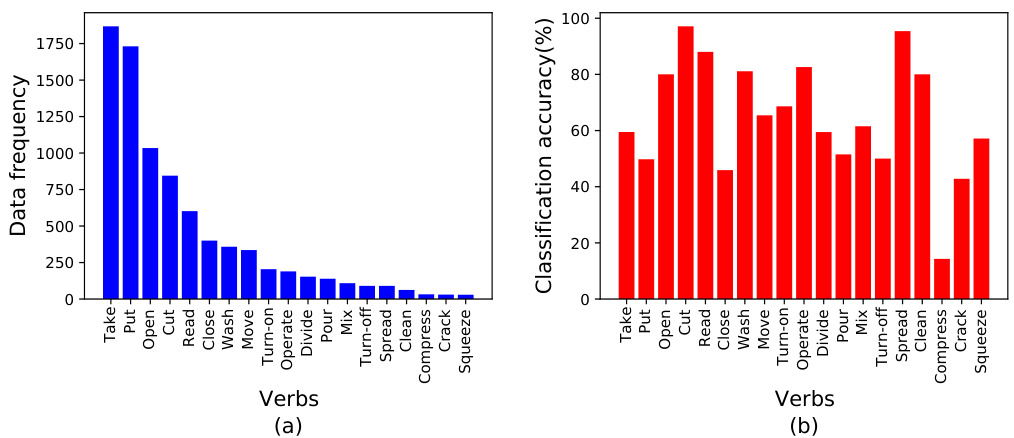
Fig. 1. (a) Class-imbalanced data distribution of EGTEA dataset. (b) Class-wise classification accuracies of a 3D-ResNeXt101 trained on the imbalanced EGTEA dataset using unweighted softmax cross-entropy loss function. It is interesting to notice that even though classes like ‘Clean’ and ‘Spread’ have very small number of data samples, the classifier finds it relatively easier to learn such classes compared to certain densely populated classes such as ‘Take’ and ‘Put’. Therefore it is not obvious to assume that the sparsely populated classes will always be the most weakly represented.
图 1: (a) EGTEA 数据集的类别不平衡数据分布。(b) 使用未加权 softmax 交叉熵损失函数在不平衡 EGTEA 数据集上训练的 3D-ResNeXt101 的逐类分类准确率。有趣的是,尽管像"Clean"和"Spread"这样的类别数据样本数量很少,但分类器发现学习这些类别比某些密集类别(如"Take"和"Put")相对更容易。因此,不能简单地假设稀疏类别总是表现最弱。
Such a strategy measures the instantaneous difficulty of each class without relying on any prior assumptions and then dynamically assigns weights to the samples of the class in proportion to the difficulty of the class. Extensive experiments on multiple datasets indicate that our class-difficulty based dynamic weighting strategy can provide a significant improvement in the performance of the commonly used loss functions under class-imbalanced situations.
该策略无需依赖任何先验假设即可测量每个类别的即时难度,随后根据类别难度动态按比例分配样本权重。在多个数据集上的大量实验表明,我们提出的基于类别难度的动态加权策略能显著提升常用损失函数在类别不平衡场景下的性能表现。
The key contributions of this paper can be summarized as follows: (1) We propose a way to measure the dynamic difficulty of each class during training and use the class-wise difficulty scores to re-balance the loss for each sample, thereby giving a class-wise difficulty-balanced (CDB) loss. (2) We show that using our weighting strategy can give commonly used loss functions (e.g., cross-entropy) a significant boost in performance on multiple class-imbalanced datasets. We conduct experiments on both image and video datasets and find that our weighting strategy works well irrespective of the data type. Our research on quantifying the dynamic difficulty of the classes and using it for weight distribution might prove useful for researchers focusing on class-imbalanced datasets.
本文的主要贡献可总结如下:(1) 我们提出了一种在训练过程中测量每个类别动态难度的方法,并利用类别难度分数重新平衡每个样本的损失,从而得到一种类别难度平衡(CDB)损失函数。(2) 我们证明采用这种加权策略可以显著提升常用损失函数(如交叉熵)在多个类别不平衡数据集上的性能。我们在图像和视频数据集上进行了实验,发现该加权策略对不同数据类型均有效。关于量化类别动态难度并将其用于权重分配的研究,可能对关注类别不平衡数据集的研究者具有参考价值。
2 Related Works
2 相关工作
As discussed in section 1, most prior works that try to solve class-imbalance can be categorized into 3 domains : (1) Data re-sampling techniques, (2) Metric learning and knowledge transfer and (3) Cost-sensitive learning methods.
如第1节所述,大多数解决类别不平衡问题的现有工作可分为三大类:(1) 数据重采样技术,(2) 度量学习和知识迁移,(3) 代价敏感学习方法。
2.1 Data Re-sampling
2.1 数据重采样
Data re-sampling techniques try to balance the number of samples among the classes by using various sampling techniques during the data pre-processing. The sampling techniques, used for the purpose, either randomly over-sample data from the minority classes or randomly under-sample data from the majority classes or both. Over-sampling from the minority classes [8,24] replicates the available data samples in order to increase the number of samples. But such a practice introduces the risk of over fitting. Synthetic Minority Over-sampling Technique (SMOTE) [7], proposed by Chawla et al., increases the number of data samples for the minority classes by creating synthetic data using interpolation among the original data points. Though SMOTE only used the minority class samples while generating data samples, later variants of SMOTE (e.g., Borderline SMOTE [18] and Safe-level SMOTE [19]) take the majority class samples into consideration as well. But such data generation techniques do not guarantee that the synthesized data points will always follow the actual data distribution of the minority classes. On the other hand, under-sampling techniques [9,25] reduce data from the majority classes and might result in cutting out some important data samples.
数据重采样技术通过在数据预处理阶段采用多种采样方法,力求平衡各类别的样本数量。这些采样技术要么对少数类数据进行随机过采样,要么对多数类数据进行随机欠采样,或者两者兼用。少数类过采样[8,24]通过复制现有数据样本来增加样本数量,但这种方法可能带来过拟合风险。Chawla等人提出的合成少数类过采样技术(SMOTE)[7]通过在原始数据点间插值生成合成数据,从而增加少数类的样本数量。尽管SMOTE在生成数据样本时仅使用少数类样本,但其后续改进版本(如Borderline SMOTE[18]和Safe-level SMOTE[19])也考虑了多数类样本。然而这类数据生成技术无法保证合成数据点始终符合少数类的真实数据分布。另一方面,欠采样技术[9,25]通过削减多数类数据来平衡样本,但可能导致部分重要数据样本丢失。
2.2 Metric Learning and Knowledge Transfer
2.2 度量学习与知识迁移
Metric learning aims to learn an embedding function that can embed data to a feature space where the inter-data relationships are preserved. Contrastive embedding [26] is learned using paired data samples to minimize the distance between the features of same class samples while maximizing the distance between different class samples. Song et al. [10] proposed a structured feature embedding based on positive and negative samples pairs in the dataset. Triplet loss [27], on the other hand, uses triplets instead of pairs, where one sample is considered the anchor. Metric learning still faces the risk of learning embedding functions biased towards the majority classes. Some recent works (e.g., OLTR [20]) have also tried to transfer knowledge from the majority classes to the minority classes either by meta learning [13] or by adding an external memory module [20]. Even though OLTR [20] performs well for long-tailed classification, as pointed out by [28], their design of external memory modules might be a non-trivial and expensive task.
度量学习的目标是学习一种嵌入函数,能够将数据映射到一个保留数据间关系的特征空间。对比嵌入 [26] 通过使用配对数据样本来学习,最小化同类样本特征之间的距离,同时最大化不同类样本之间的距离。Song等人 [10] 提出了一种基于数据集中正负样本对的结构化特征嵌入方法。而三元组损失 [27] 则使用三元组而非配对样本,其中一个样本被视为锚点。度量学习仍面临学习偏向多数类的嵌入函数的风险。最近的一些工作(如OLTR [20])尝试通过元学习 [13] 或添加外部记忆模块 [20] 将知识从多数类迁移到少数类。尽管OLTR [20] 在长尾分类中表现良好,但如 [28] 所指出的,其外部记忆模块的设计可能是一项复杂且成本高昂的任务。
2.3 Cost-Sensitive Learning
2.3 代价敏感学习
Cost-sensitive learning techniques try to penalize the DNN higher for making prediction mistakes on certain data samples than on the others. To achieve that, different weights are assigned to different samples and the penalty incurred on each data sample is scaled up/down using the corresponding weight. Research in this domain mainly target to find an effective way to assign these weights to the samples. To solve class-imbalance, majority of the works propose techniques that assign higher weights to the minority class samples. Such techniques ensure that the DNN gets higher penalty for making mistakes on the minority class samples. One such simple and commonly used weight distribution technique is to use the inverse class-frequencies as the weights for the samples each class [21,23]. Later variants of this technique [22] use a smoothed version of the square root of class-frequencies for the weight distribution. Class-balanced loss [15] proposed by Lin et al. calculates the effective number of samples of each class and uses it to assign weights to the samples. All of the above mentioned works assume that the minority classes are always the most weakly represented classes and therefore needs high weights. But that assumption might not always be true because certain minority class might be sufficiently represented by a small number of samples. Giving high weights to the samples of such classes might cause drop in overall performance. Therefore, Tsung-Yi et al. proposed a sample-based weighting technique called “Focal loss” [14], where each sample is assigned a weight based on it’s difficulty. The difficulty of each sample is quantified in terms of the loss incurred by the DNN on that sample, where more lossy samples imply more difficult samples. Though focal loss [14] was originally proposed for dense object detection tasks, it has also become popular in class-imbalanced classification tasks [15]. The minority classes are expected to have more difficult samples compared to the majority classes and therefore get high weights by focal loss. Indeed the proportion of difficult samples in a minority class is more than that in the majority class. However, in terms of absolute number of difficult samples, the majority class surpasses the minority class, as it is much more populated than the minority class. Therefore, giving high weights to all difficult samples irrespective of their classes still biases the DNN’s performance.
成本敏感学习技术试图通过在某些数据样本上做出错误预测时对DNN施加更高的惩罚,而对其他样本则施加较低的惩罚。为实现这一点,不同样本被赋予不同的权重,每个数据样本的惩罚会根据相应权重进行放大或缩小。该领域的研究主要致力于寻找一种有效的方法来为样本分配这些权重。为解决类别不平衡问题,大多数研究提出了为少数类样本分配更高权重的技术。这类技术确保DNN在少数类样本上犯错时受到更严厉的惩罚。其中一种简单且常用的权重分配技术是使用类别频率的倒数作为每个类别样本的权重[21,23]。该技术的后续变体[22]则使用类别频率平方根的平滑版本进行权重分配。Lin等人提出的类别平衡损失[15]通过计算每个类别的有效样本数来分配样本权重。上述所有研究都假设少数类始终是代表性最弱的类别,因此需要高权重。但这一假设未必总是成立,因为某些少数类可能仅需少量样本即可充分表示。对此类样本赋予高权重可能导致整体性能下降。因此,Tsung-Yi等人提出了一种基于样本的权重分配技术"焦点损失(Focal loss)"[14],根据样本难度为每个样本分配权重。样本难度通过DNN在该样本上的损失量化,损失越大表示样本越难。虽然焦点损失[14]最初是为密集目标检测任务提出的,但也在类别不平衡分类任务中广受欢迎[15]。与多数类相比,少数类预期会包含更多困难样本,因此通过焦点损失获得更高权重。事实上,少数类中困难样本的比例确实高于多数类。然而就困难样本的绝对数量而言,多数类因其样本基数更大而超过少数类。因此,不分类别地为所有困难样本赋予高权重仍会导致DNN性能偏差。
Our work also lies in the regime of cost-sensitive learning. We propose a dynamic weighting system that dynamically assigns weights to each sample of each class based on the instantaneous difficulty of the class, rather than that of each sample, as perceived by the DNN. Our weighting system helps to boost the performance of commonly used loss functions (e.g., cross-entropy loss) in class-imbalanced situations.
我们的工作也属于成本敏感学习范畴。我们提出了一种动态加权系统,该系统基于深度神经网络感知的类别瞬时难度(而非样本难度)动态分配每个类别样本的权重。该加权系统能有效提升常用损失函数(如交叉熵损失)在类别不平衡场景下的性能。
3 Proposed Method
3 研究方法
3.1 Measuring Class Difficulty
3.1 衡量类别难度
Human beings use the metric ‘difficulty’ majorly to give a qualitative description of things, for example “this task is very difficult” or “this game is so easy”. Similar behavior can also be seen in neural networks where they find some parts of a task much more difficult to perform compared to the others. For example, while training on a multi-class classification task, the classifier will find some classes easier to learn than the others. We propose to measure the difficulty of each class as perceived by the DNN and use it as clue to determine the weights for the samples. But, as difficulty is a qualitative metric, there is no direct way to add a quantitative value to it. Humans tend to classify a task as difficult, if they can not perform well in it. We use a similar approach to use the neural network’s performance to measure the difficulty of classes. During training, the neural network’s performance for each class is measured on a validation data set, which is then used to calculate the class-wise difficulty. The neural network’s performance for any class $c$ is measured as its classification accuracy on class $c$ , $A_{c}~=~n_{c}/N_{c}$ , where $N_{c}$ denotes the total number of samples of class $c$ in validation data and $n_{c}$ denotes the number of class $c$ samples in validation data that the model classifies correctly. Then the difficulty of class $c$ , $d_{c}$ , is measured as $d_{c}=1-A_{c}$ . A neural network’s perception of “how much a class is difficult to learn” changes as the training process of the network progresses. With time, the network’s performance for each class improves and as a result, the perceived difficulty of each class also reduces. Therefore, we calculate the class-difficulties as a function of time as well. The difficulty of class $c$ after training time (i.e., time during training) $t$ can be calculated as
人类主要使用“难度”这一指标对事物进行定性描述,例如“这项任务非常困难”或“这个游戏很简单”。类似行为也存在于神经网络中,它们会发现任务的某些部分比其他部分更难处理。例如,在进行多类别分类任务训练时,分类器会发现某些类别比其他类别更容易学习。我们提出通过深度神经网络(DNN)感知的各类别难度作为样本权重的确定依据。但由于难度是定性指标,无法直接赋予量化值。人类倾向于将表现不佳的任务归类为困难任务,我们采用类似思路,利用神经网络的表现来衡量类别难度。训练过程中,神经网络在验证数据集上对每个类别的表现被量化为分类准确率 $A_{c}~=~n_{c}/N_{c}$ ,其中 $N_{c}$ 表示验证数据中类别 $c$ 的总样本数, $n_{c}$ 表示模型正确分类的类别 $c$ 样本数。随后,类别 $c$ 的难度 $d_{c}$ 计算为 $d_{c}=1-A_{c}$ 。神经网络对“类别学习难度”的感知会随训练进程动态变化:随着时间推移,网络对各類别的表现提升,其感知难度相应降低。因此,我们将类别难度表述为时间的函数,训练时长 $t$ 后的类别 $c$ 难度可计算为
$$
d_{c,t}=1-A_{c,t},
$$
$$
d_{c,t}=1-A_{c,t},
$$
where $A_{c,t}$ is the neural network’s classification accuracy for class $c$ on the validation data after training time $t$ .
其中 $A_{c,t}$ 表示神经网络在训练时间 $t$ 后对验证数据中类别 $c$ 的分类准确率。
3.2 Difficulty-Based Weight Distribution
3.2 基于难度的权重分配
Once the class-wise difficulty is quantified, then it can be used to assign weights to the classes during training. It is fairly obvious that the classes, that are difficult to learn should be given higher weights compared to the easier classes. Therefore the weight for class $c$ after training time $t$ can be calculated as
一旦量化了各类别的学习难度,便可在训练过程中为不同类别分配权重。显然,相较于简单类别,难学习的类别应被赋予更高权重。因此,训练时间 $t$ 后类别 $c$ 的权重可计算为
$$
w_{c,t}=(d_{c,t})^{\tau}=(1-A_{c,t})^{\tau},
$$
$$
w_{c,t}=(d_{c,t})^{\tau}=(1-A_{c,t})^{\tau},
$$
where $d_{c,t}$ is the difficulty of class $c$ after time $t$ and $\tau$ is a hyper-parameter. The weight distribution $w_{t}={w_{1,t},w_{2,t},\dots,w_{C,t}}$ over all $C$ classes can be computed by repeating Equation 2 for all classes.
其中 $d_{c,t}$ 表示时间 $t$ 后类别 $c$ 的难度,$\tau$ 是一个超参数。通过对所有 $C$ 个类别重复公式 2,可以计算出所有类别上的权重分布 $w_{t}={w_{1,t},w_{2,t},\dots,w_{C,t}}$。
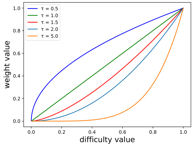
Fig. 2. Effect of changing $\tau$ on the difficulty-based weight distribution. Increasing value of $\tau$ puts heavier weights on the samples of the classes with higher difficulty, while lowering weights for the easier classes.
图 2: 改变 $\tau$ 对基于难度权重分布的影响。增大 $\tau$ 值会给难度较高的类别样本分配更大权重,同时降低简单类别的权重。
The hyper-parameter $\tau$ is introduced to control how much we down-weight the samples of the easy classes. Increasing value of $\tau$ relatively increases the classifier’s focus on the difficult classes.
引入超参数 $\tau$ 来控制对简单类样本的降权程度。增大 $\tau$ 值会相对增强分类器对困难类的关注。
Fig. 2 shows how change in the value of $\tau$ changes the weight values for classes of different difficulties. Its effect is almost similar to that of the focusing parameter $\gamma$ in focal loss [14]. The performance of our proposed method varies significantly with change in value of $\tau$ and the best value for $\tau$ differs from dataset to dataset. Unfortunately, the only way to search for the best value of $\tau$ is by trial and error. To avoid that, we propose a way to dynamically update the value of $\tau$ . For dynamically updating $\tau$ , the value of $\tau$ after training time $t$ is calculated as
图 2: 展示了参数 $\tau$ 值的变化如何影响不同难度类别权重值的调整。其效果与焦点损失 [14] 中的聚焦参数 $\gamma$ 几乎相似。我们提出方法的性能随 $\tau$ 值变化而显著波动,且最佳 $\tau$ 值因数据集而异。遗憾的是,寻找最佳 $\tau$ 值的唯一方法是通过试错。为避免这种情况,我们提出了一种动态更新 $\tau$ 值的方法。对于动态更新 $\tau$,训练时间 $t$ 后的 $\tau$ 值计算公式为
$$
\tau_{t}=\frac{2}{1+\exp(-b_{t})},
$$
$$
\tau_{t}=\frac{2}{1+\exp(-b_{t})},
$$
where $b_{t}$ measures the bias in the performance of the classifier over $C$ classes as
其中 $b_{t}$ 衡量分类器在 $C$ 个类别上的性能偏差为
$$
b_{t}=\frac{\operatorname*{max}{c=1,2,\ldots,C}A_{c,t}}{\operatorname*{min}{c^{\prime}=1,2,\ldots,C}A_{c^{\prime},t}+\epsilon}-1.
$$
$$
b_{t}=\frac{\operatorname*{max}{c=1,2,\ldots,C}A_{c,t}}{\operatorname*{min}{c^{\prime}=1,2,\ldots,C}A_{c^{\prime},t}+\epsilon}-1.
$$
In Equation 4, $\epsilon$ is a small positive value $=+0.0001$ ) introduced to handle situations where $\mathrm{min}{c^{\prime}=1,2,...,C}A_{c^{\prime},t}=0$ . Equation 3 increases the value of $\tau$ when the classification performance of the classifier is highly biased (i.e., high $b_{t}$ ) and decreases it in case of low bias (i.e., less $b_{t}$ ).
在公式4中,$\epsilon$ 是一个小的正值 $=+0.0001$ ),用于处理 $\mathrm{min}{c^{\prime}=1,2,...,C}A_{c^{\prime},t}=0$ 的情况。公式3在分类器性能高度偏差(即高 $b_{t}$ )时增加 $\tau$ 的值,在偏差较低(即较小 $b_{t}$ )时减小它。
3.3 Class-Wise Difficulty-Balanced Softmax Cross-Entropy Loss
3.3 类别难度平衡的Softmax交叉熵损失
Suppose when an input data is fed to the classifier after training time $t$ during training, the predicted output of the classifier for all $C$ classes are $z_{t}=$
假设在训练时间 $t$ 后将输入数据输入分类器时,分类器对所有 $C$ 个类别的预测输出为 $z_{t}=$
${z_{1,t},z_{2,t},\ldots,z_{C,t}}$ . The probability distribution $p_{t}={p_{1,t},p_{2,t},...,p_{C,t}}$ over all the classes is computed using the softmax function, which is
${z_{1,t},z_{2,t},\ldots,z_{C,t}}$。类别概率分布 $p_{t}={p_{1,t},p_{2,t},...,p_{C,t}}$ 通过softmax函数计算得出,其公式为
$$
p_{j,t}=\frac{\exp{z_{j,t}}}{\sum_{i=1}^{C}\exp{z_{i,t}}}\forall j\in{1,2,\ldots,C}.
$$
$$
p_{j,t}=\frac{\exp{z_{j,t}}}{\sum_{i=1}^{C}\exp{z_{i,t}}}\forall j\in{1,2,\ldots,C}.
$$
For an input data sample of class $k$ , cross-entropy (CE) loss function com- putes the loss after training time $t$ as
对于一个类别为 $k$ 的输入数据样本,交叉熵损失函数 (cross-entropy loss) 在训练时间 $t$ 后计算损失值为
$$
\mathrm{CE}(p_{t},k)=-\log p_{k,t}.
$$
$$
\mathrm{CE}(p_{t},k)=-\log p_{k,t}.
$$
For the same input data sample, our class-wise difficulty-balanced softmax crossentropy (CDB-CE) loss function computes the loss after training time $t$ as
对于相同的输入数据样本,我们的类难度平衡softmax交叉熵 (CDB-CE) 损失函数在训练时间 $t$ 后计算损失为
$$
\mathrm{CDB-CE}(w_{t},p_{t},k)=-w_{k,t}\log p_{k,t}.
$$
$$
\mathrm{CDB-CE}(w_{t},p_{t},k)=-w_{k,t}\log p_{k,t}.
$$
To make the weights time-dependent, we calculate them after each epoch using the model’s class-wise validation accuracy.
为了使权重具有时间依赖性,我们在每个训练周期后根据模型的类别验证准确率来计算它们。
4 Experiments
4 实验
To demonstrate our proposed solution’s ability to generalize to any data-type or dataset, we evaluate the effectiveness of our solution on 4 different datasets namely MNIST, long-tailed CIFAR, ImageNet-LT and EGTEA. MNIST, longtailed CIFAR and ImageNet-LT are image datasets while EGTEA is a video dataset.
为验证我们提出的解决方案能够泛化到任意数据类型或数据集,我们在4个不同数据集上评估了方案有效性:MNIST、长尾CIFAR、ImageNet-LT和EGTEA。其中MNIST、长尾CIFAR和ImageNet-LT为图像数据集,EGTEA为视频数据集。
4.1 Datasets
4.1 数据集
MNIST. From the standard MNIST handwritten digit recognition dataset [1], we generate a class-imbalanced binary classification task using a subset of the dataset. The experimental setup is exactly same as given in [29]. We select a total of 5000 training images of class ‘4’ and ‘9’ where ‘9’ is chosen as the majority class. We calculate the ‘majority class ratio’ as
MNIST。我们从标准MNIST手写数字识别数据集[1]中生成一个类别不平衡的二分类任务,使用该数据集的子集。实验设置与[29]中给出的完全相同。我们总共选择了5000张类别为"4"和"9"的训练图像,其中"9"被选为多数类。计算"多数类比例"的公式为
$$
\mathrm{majority class ratio}={\frac{\mathrm{no. of training samples in majority class}}{\mathrm{no. of training~samples}}}.
$$
多数类比例 = (多数类训练样本数 / 总训练样本数)
Increasing the majority class ratio increases the imbalance in the training dataset. We also use a validation set which is created by selecting 500 images for each of the two classes from the original dataset but these images are different from the 5000 images selected for training. A test set was also created by randomly selecting 800 images for each of the classes from the original MNIST test set.
增加多数类比例会加剧训练数据集的不平衡性。我们还构建了一个验证集,从原始数据集中为两个类别各选取500张图像(这些图像与用于训练的5000张图像不同)。测试集则是从原始MNIST测试集中为每个类别随机抽取800张图像构成。
Long-Tailed CIFAR. We conduct experiments on long-tailed CIFAR-100 [2]. First a validation set was created from the original training set by randomly selecting 50 images per class. After the separation of the validation set, the remaining images in the training set were used to create a long-tailed version of the dataset using the exact same procedure as stated in [15]. The number of training images per class are reduced following an exponential function $n=n_{c}\mu^{c}$ , where $c$ is the 0-based index of the class and $n_{c}$ is the remaining number of training images of class $c$ after separation of the validation set and $\mu\in(0,1)$ . Similar to [15], the ‘imbalance’ factor of a dataset is defined as the number of training samples in the largest class divided by that of the smallest class. The test set used for experiment is exactly same as the original CIFAR test set available and is a balanced set.
长尾CIFAR。我们在长尾CIFAR-100 [2]上进行了实验。首先从原始训练集中随机选取每类50张图像创建验证集。分离验证集后,使用与[15]完全相同的流程,将训练集中剩余的图像生成长尾版本数据集。每类训练图像数量按指数函数$n=n_{c}\mu^{c}$递减,其中$c$为类别索引(从0开始),$n_{c}$为分离验证集后类别$c$剩余的训练图像数,$\mu\in(0,1)$。参照[15],数据集的"不平衡"因子定义为最大类训练样本数与最小类的比值。实验使用的测试集与原始CIFAR测试集完全相同,为平衡数据集。
ImageNet-LT. We also conduct experiments on the long-tailed version of the original ImageNet-2012 [3], as constructed in [20]. It comprises of 115,800 images from 1000 categories, where the most frequent class has 1280 image samples and the least frequent class has only 5 images. The test set is balanced. The split constructed by [20] also provides a validation set that is separate from the test set and training set.
ImageNet-LT。我们还在原始ImageNet-2012[3]的长尾版本上进行了实验,该版本由[20]构建。它包含来自1000个类别的115,800张图像,其中最常见类别有1280个图像样本,最不常见类别仅有5张图像。测试集是平衡的。[20]构建的分割还提供了一个独立于测试集和训练集的验证集。
EGTEA. We also conduct experiments on the EGTEA Gaze+ dataset [30]. This is an egocentric dataset that contains trimmed video clips of many kitchenrelated actions. These video clips are extracted segments from longer videos that were collected by 32 different subjects. Each video clip is assigned a single action label and the challenge is to train a classifier to classify the actions from the provided video clips. Each action label is made up of a verb and a set of nouns (e.g., the action ‘Wash Plate’ is made up of the verb ‘Wash’ and noun ‘Plate’). The noun classification task is very similar to the image classification task. So, for our experiments, we focus on the verb classification in order to test our proposed method on diverse tasks. This dataset has 19 different verb classes (e.g., ‘Open’, ‘Wash’ etc.). EGTEA Gaze $^+$ [30] is inherently class-imbalanced. Fig. 1(a) shows the data distribution of the EGTEA dataset. For our experiments, we use the split1 of the EGTEA dataset (8299 training video clips and 2022 testing video clips). We create our validation set by using the training video clips from subjects P20 to P26, resulting in 1927 validation video clips and 6372 training clips.
EGTEA。我们还在EGTEA Gaze+数据集[30]上进行了实验。这是一个以自我为中心的数据集,包含许多厨房相关动作的修剪视频片段。这些视频片段是从32名不同受试者采集的长视频中提取的片段。每个视频片段都有一个动作标签,挑战在于训练一个分类器,根据提供的视频片段对动作进行分类。每个动作标签由一个动词和一组名词组成(例如,动作"Wash Plate"由动词"Wash"和名词"Plate"组成)。名词分类任务与图像分类任务非常相似。因此,在我们的实验中,我们专注于动词分类,以便在不同的任务上测试我们提出的方法。该数据集有19个不同的动词类别(例如"Open"、"Wash"等)。EGTEA Gaze$^+$[30]本质上存在类别不平衡问题。图1(a)显示了EGTEA数据集的数据分布。在我们的实验中,我们使用EGTEA数据集的split1(8299个训练视频片段和2022个测试视频片段)。我们通过使用受试者P20到P26的训练视频片段创建验证集,得到1927个验证视频片段和6372个训练片段。
4.2 Implementation Details
4.2 实现细节
We use a LeNet-5 [31] model for MNIST unbalanced binary classification experiments following [29]. The model is trained for 4000 epochs on a single NVIDIA GeForce GTX 1080 GPU with a batch size of 100. As optimizer, we use Stochastic Gradient Descent (SGD) with momentum of 0.9, weight decay of 0.0005 and an initial learning rate of 0.001, which is decayed by 0.1 after 3000 epochs. The trained model is tested on the balanced test set.
我们采用LeNet-5 [31]模型进行MNIST不平衡二分类实验,方法参照[29]。该模型在NVIDIA GeForce GTX 1080单显卡上训练4000轮次,批量大小为100。优化器采用带动量(0.9)的随机梯度下降法(SGD),权重衰减率为0.0005,初始学习率设为0.001并在3000轮次后衰减为原值的0.1倍。最终模型在平衡测试集上进行评估。
For experiments on long-tailed CIFAR, we follow the exact same implementation strategy as provided in [15]. We train a ResNet-32 [32] model for 200 epochs using a batch size of 128 on 4 NVIDIA Titan X GPUs. We use SGD optimizer with momentum 0.9 and weight decay of 0.0005. An initial learning rate of 0.1 is used, which is decayed by 0.01 after 160 and 180 epochs.
在长尾CIFAR数据集上的实验中,我们完全遵循[15]提供的实现策略。使用4块NVIDIA Titan X GPU训练ResNet-32 [32]模型200个周期,批量大小为128。采用SGD优化器,动量0.9,权重衰减0.0005。初始学习率为0.1,并在160和180周期后衰减0.01。
For experiments on ImageNet-LT, we use the same setup as in [20]. We use ResNet-10 [32] model for the purpose. The trained model is tested on the balanced test data.
在ImageNet-LT上的实验中,我们采用与[20]相同的设置。为此我们使用ResNet-10 [32]模型。训练好的模型在平衡测试数据上进行评估。
For EGTEA dataset, we use a 3D-ResNeXt101 [33,34] model and train it for 100 epochs on 8 NVIDIA Titan X GPUs using a batch size of 32. SGD with momentum 0.9 is used with a weight decay of 0.0005 and an initial learning rate of 0.001, which is decayed by 0.1 after 60 epochs. During training, we sample 10 RGB frames from each video clip by dividing the clip into 10 equal segments followed by randomly selecting one RGB frame from each segment. We use random-cropping, random-rotating and horizontal-flipping as data augmentation. Training input size is $10\times3\times224\times2{:}24$ . During testing and validation, we sample 10 RGB frames at equal intervals from each video clip.
对于EGTEA数据集,我们采用3D-ResNeXt101 [33,34]模型,在8块NVIDIA Titan X GPU上以32的批量大小训练100个周期。使用带动量0.9的SGD优化器,权重衰减为0.0005,初始学习率为0.001,并在60个周期后衰减为0.1倍。训练时,我们将每个视频片段均分为10段,每段随机选取1帧RGB图像,共采样10帧。数据增强采用随机裁剪、随机旋转和水平翻转。训练输入尺寸为$10\times3\times224\times2{:}24$。测试和验证阶段,我们从每个视频片段中等间隔采样10帧RGB图像。
We use PyTorch [35] framework for all our implementations. For all datasets, our CDB-CE loss implementation calculates the class-wise weights after every epoch using the model’s class-wise validation accuracy.
我们使用PyTorch [35] 框架实现所有实验。对于所有数据集,我们的CDB-CE损失实现会在每个epoch结束后根据模型的类别验证准确率计算类别权重。
4.3 Results on Unbalanced MNIST Binary Classification
4.3 非平衡MNIST二分类结果
Similar to [29], we increase the majority class ratio defined in Equation 8 from 0.9 to 0.995 by increasing the number of training samples of majority class, while keeping the total number of training samples constant at 5000. Following implementation details of [29], we retrain LeNet-5 [31] for each majority class ratio using different loss functions and compare the error rate of the trained model on the test set. Table 1 compares the effect of increasing majority class ratio on the test error rates of LeNet-5, trained using various weighted and unweighted loss functions. For comparison, we use the mean and standard deviation of the classification error rates achieved over 10 runs using random splits. The compared loss functions include (1) Unweighted Cross-Entropy(CE) , which uses an unweighted softmax cross-entropy loss function to train the model; (2) inverse class-frequency weighting (IFW) [23], which uses a weighted softmax cross-entropy loss function where the weight for each class is calculated using the inverse of it’s frequency; (3) Focal loss [14], Class Balanced(CB) loss [15], Equalization loss (EQL) [16] and L2RW [29] are state-of-the-art loss functions.
与[29]类似,我们通过增加多数类别的训练样本数量,将公式8中定义的多数类别比例从0.9提升至0.995,同时保持训练样本总数恒定在5000。遵循[29]的实现细节,我们针对每个多数类别比例使用不同损失函数重新训练LeNet-5[31],并比较训练模型在测试集上的错误率。表1比较了增加多数类别比例对LeNet-5测试错误率的影响,模型采用多种加权和非加权损失函数进行训练。为便于比较,我们使用随机划分10次运行所得分类错误率的均值与标准差。对比的损失函数包括:(1) 非加权交叉熵(CE),使用未加权的softmax交叉熵损失函数训练模型;(2) 逆类别频率加权(IFW)[23],采用加权softmax交叉熵损失函数,其中每个类别的权重按其频率倒数计算;(3) 焦点损失(Focal loss)[14]、类别平衡(CB)损失[15]、均衡损失(EQL)[16]和L2RW[29]等前沿损失函数。
As can be seen from Table 1, our class-wise difficulty-balanced cross-entropy (CDB-CE) loss function performs better than the others. But to ensure a good performance, it is important to select an appropriate value of $\tau$ . Hence we conduct another experiment to investigate the effect of changing $\tau$ on the performance of our method. For that, we compare the performance of our CDB-CE loss function for different values of $\tau$ and different majority class ratios. The results of the experiment are listed in Table 2.
从表1可以看出,我们的类难度平衡交叉熵(CDB-CE)损失函数表现优于其他方法。但要确保良好性能,选择合适的$\tau$值至关重要。为此我们进行了另一项实验,研究改变$\tau$对我们方法性能的影响。实验中比较了不同$\tau$值和不同多数类比例下CDB-CE损失函数的性能表现,结果列于表2。
As can be seen from Table 2, increasing value of $\tau$ initially helps in improving the performance of our method but after a certain point, it leads to a drop in the performance. We believe that the drop comes due to the excessive downweighting of the samples of the easy classes. In Table 2, our method works well over a wide range of $\tau$ values. The best value for $\tau$ varies even with the majority class ratio. But one interesting thing to notice is that even though dynamically updating $\tau$ does not always give the best performance, it’s performance is never too far from the best and it consistently outperforms all the existing methods listed in Table 1. Therefore, dynamically updating $\tau$ can be a default choice to select the value of $\tau$ in case one wants to avoid trial and error searching for the best $\tau$ .
从表2可以看出,增大$\tau$值最初有助于提升我们方法的性能,但超过某个临界点后会导致性能下降。我们认为这种下降是由于对简单类别样本的过度降权所致。在表2中,我们的方法在$\tau$值较大范围内都表现良好。$\tau$的最佳值甚至会随多数类比例而变化。但值得注意的是,虽然动态更新$\tau$并不总能获得最佳性能,但其表现始终与最优值相差不大,并且持续优于表1所列的所有现有方法。因此,若想避免通过试错法寻找最佳$\tau$值,动态更新$\tau$可以作为一个默认选择。
Table 1. Mean and standard deviation of classification error rates ( $%$ ) of LeNet-5 [31] trained for MNIST [1] imbalanced binary classification using different loss functions for different majority class ratios. Here we show the best results obtained by each of the loss functions in our implementation. For class-wise difficulty-balanced softmax cross-entropy (CDB-CE) loss (Ours), we report the results with dynamically updated $\tau$ .
表 1. 使用不同损失函数在不同多数类比例下训练 LeNet-5 [31] 进行 MNIST [1] 不平衡二分类的分类错误率均值及标准差 ( $%$ )。此处展示我们实现中各损失函数取得的最佳结果。对于类别难度平衡的 softmax 交叉熵损失 (CDB-CE) (Ours),我们报告了动态更新 $\tau$ 时的结果。
| Maj.class ratio | 0.9 | 0.95 | 0.98 | 0.99 | 0.995 |
|---|---|---|---|---|---|
| Unweighted CE | 1.50 ± 0.51 | 2.36±0.46 | 5.09 ± 0.41 | 8.59± 0.41 | 14.35 ±1.10 |
| IFW [23] | 1.16 ± 0.40 | 1.74 ± 0.31 | 3.13 ± 0.74 | 6.01 ± 0.56 | 8.94 ± 0.70 |
| Focal Loss s [14] | 1.74 ± 0.26 | 2.78±0.29 | 6.67± 0.63 | 11.11 ± 1.20 | 17.17 ± 0.86 |
| CB Loss [15] | 1.07±0.23 | 1.79 ±0.39 | 3.58±0.71 | 5.88±1.20 | 8.61 ± 1.11 |
| EQL [16] | 1.49 ± 0.34 | 2.26 ± 0.41 | 2.43 ± 0.14 | 2.60±0.33 | 3.71 ± 0.41 |
| L2RW [29] | 1.24 ± 0.69 | 1.76 ± 1.12 | 2.06 ± 0.85 | 2.63 ± 0.65 | 3.94 ±1.23 |
| CDB-CE(Ours) | 0.74±0.14 | 1.27±0.33 | 1.65 ±0.26 | 2.39±0.41 | 3.71±0.27 |
Table 2. Mean and standard deviation of classification error rates $(%$ ) of LeNet-5 [31] trained for MNIST imbalanced binary classification using our CDB-CE loss with different values of $\tau$ For dynamically updating $^{\circ}$ (last row), we update the value of $\tau$ after every epoch as given in Equation 3.
表 2. 使用不同 $\tau$ 值的 CDB-CE 损失训练 MNIST 不平衡二分类任务时 LeNet-5 [31] 的分类错误率均值及标准差 $(%$ ) 对于动态更新 $^{\circ}$ (最后一行), 我们按照公式 3 在每个 epoch 后更新 $\tau$ 值。
| Maj. class ratio | 0.9 | 0.95 | 0.98 | 0.99 | 0.995 |
|---|---|---|---|---|---|
| T=0.5 | 1.06 ±0.34 | 1.43 ±0.24 | 1.93±0.27 | 2.59±0.44 | 4.03 ±0.41 |
| T = 1.0 | 0.90±0.27 | 1.38±0.20 | 1.86 ±0.30 | 2.49±0.57 | 3.94±0.36 |
| T = 1.5 | 0.85±0.19 | 1.35±0.31 | 1.71±0.28 | 2.31±0.38 | 3.54±0.25 |
| T = 2.0 | 0.75±0.15 | 1.21±0.32 | 1.75±0.36 | 2.23±0.34 | 3.65 ±0.41 |
| T =5.0 | 0.88±0.25 | 1.19±0.36 | 2.00±0.32 | 2.51 ±0.41 | 3.78±0.43 |
| T = 7.0 | 0.96±0.20 | 1.20 ±0.20 | 2.04 ±0.30 | 2.64 ±0.40 | 4.13±0.37 |
| dyn. updated T | 0.74±0.14 | 1.27±0.33 | 1.65±0.26 | 2.39 ±0.41 | 3.71±0.27 |
4.4 Results on Long-Tailed CIFAR-100
4.4 长尾 CIFAR-100 上的结果
We conduct extensive experiments on long-tailed CIFAR-100 dataset [2,15] as well. ResNet-32 [32] is retrained for different imbalance factors in the training dataset, using different loss functions. Table 3 reports the classification accuracy( $%$ ) of each such trained model on the CIFAR-100 test set. We compare the results of our method with that of Focal loss [14], Class-Balanced loss [15], L2RW [29], Meta-Weight Net [36] and Equalization loss [16].
我们在长尾CIFAR-100数据集[2,15]上也进行了大量实验。使用不同损失函数对ResNet-32[32]在训练数据集的不同不平衡因子下进行重新训练。表3报告了这些训练模型在CIFAR-100测试集上的分类准确率( $%$ )。我们将本方法的结果与Focal loss[14]、Class-Balanced loss[15]、L2RW[29]、Meta-Weight Net[36]和Equalization loss[16]进行了对比。
As can be seen from Table 3, our CDB-CE loss with dynamically updated $\tau$ provides better performance than the others in most cases. But as stated in
从表3可以看出,在大多数情况下,我们采用动态更新$\tau$的CDB-CE损失函数比其他方法表现更优。但正如
Table 3. Top-1 classification accuracy ( $%$ ) of ResNet-32 trained on long-tailed CIFAR100 training data. $^\dagger$ means that the result has been copied from the origin paper [15,36,37]. For CDB-CE loss (Ours), we report the results with dynamically updated $\tau$ .
表 3. 在长尾CIFAR100训练数据上训练的ResNet-32的Top-1分类准确率( $%$ )。$^\dagger$表示结果来自原论文[15,36,37]。对于CDB-CE损失(本方法),我们报告了动态更新$\tau$的结果。
| 不平衡率 | 200 | 100 | 50 | 20 | 10 |
|---|---|---|---|---|---|
| Focal loss [14] | 35.62 | 38.41 | 44.32 | 51.95 | 55.78 |
| Class-Balanced [15] | 36.23 | 39.60 | 45.32 | 52.99 | 57.99 |
| L2RW [29] | 33.38 | 40.23 | 44.44 | 51.64 | 53.73 |
| Meta-Weight Net [36] | 37.91 | 42.09 | 46.74 | 54.37 | 58.46 |
| Equalization loss [16] | 37.34 | 40.54 | 44.70 | 54.12 | 58.32 |
| LDAM-DRW [37] | - | 42.04 | - | - | 58.71 |
| CDB-CE (本方法) | 37.40 | 42.57 | 46.78 | 54.22 | 58.74 |
Table 4. Top-1 classification accuracy ( $%$ ) of ResNet-32 trained using class-wise difficulty-balanced cross-entropy (ours) loss function for different values of $\tau$ . $\tau=0$ means the original unweighted softmax cross-entropy loss function.
表 4: 使用类间难度平衡交叉熵损失函数(本文方法)训练的ResNet-32在不同$\tau$值下的Top-1分类准确率($%$)。$\tau=0$表示原始未加权的softmax交叉熵损失函数。
| 不平衡比例 | 200 | 100 | 50 | 20 | 10 |
|---|---|---|---|---|---|
| $\tau=0$ | 34.95 | 38.21 | 43.89 | 51.34 | 55.65 |
| $\tau=0.5$ | 37.21 | 41.26 | 46.13 | 54.60 | 58.29 |
| $\tau=1.0$ | 37.99 | 41.67 | 46.45 | 53.48 | 59.47 |
| $\tau=1.5$ | 37.63 | 42.70 | 47.09 | 52.74 | 58.68 |
| $\tau=2.0$ | 37.03 | 42.44 | 46.94 | 53.00 | 58.65 |
| $\tau=5.0$ | 36.81 | 40.62 | 45.45 | 51.67 | 54.48 |
| 动态调整$\tau$ | 37.40 | 42.57 | 46.78 | 54.22 | 58.74 |
Section 4.3, the results of our method depend highly on the value of $\tau$ . Hence, we conduct a further study of how the performance of our method varies on the long-tailed CIFAR-100 dataset with the change in $\tau$ . The results are shown in Table 4.
第4.3节中,我们方法的结果高度依赖于 $\tau$ 的取值。因此,我们进一步研究了在长尾CIFAR-100数据集上,方法性能如何随 $\tau$ 的变化而变化。结果如表4所示。
Using $\tau=0$ makes our CDB-CE loss drop back to the original unweighted softmax cross-entropy loss function. From Table 4, almost a wide range of values for $\tau$ helps our weighted loss to get better results than the baseline of $\tau=0$ . Again the interesting thing is even though dynamically updating $\tau$ does not give the best results, it’s performance is not far from the best and it outperforms existing methods of Table 3 in majority of the cases.
使用 $\tau=0$ 会使我们的 CDB-CE 损失函数退化为原始的未加权 softmax 交叉熵损失函数。从表 4 可以看出,在 $\tau$ 取较宽泛的数值范围时,加权损失函数都能获得优于 $\tau=0$ 基线的结果。值得注意的是,虽然动态更新 $\tau$ 未能取得最佳效果,但其性能与最优结果相差无几,并且在大多数情况下优于表 3 中的现有方法。
Table 5. Top-1 classification accuracy ( $%$ ) of ResNet-10 on ImageNet-LT for different methods. $^\dagger$ means that the result has been copied from the origin paper [16,20,28].
表 5: ResNet-10 在 ImageNet-LT 上不同方法的 Top-1 分类准确率 ( $%$ )。 $^\dagger$ 表示结果来自原论文 [16,20,28]。
| 方法 | Top-1 准确率(%) |
|---|---|
| Focal loss t [14] | 30.50 |
| OLTR t [20] | 35.60 |
| Joint training ↑[28] | 34.80 |
| Equalization loss ↑ [16] | 36.44 |
| OLTR [20] + CDB-CE (Ours) | 36.70 |
| Joint training [28]+ CDB-CE (Ours) | 37.10 |
| CDB-CE (Ours) | 38.49 |
4.5 Results on ImageNet-LT
4.5 ImageNet-LT 上的结果
We compare the performance of our method on ImageNet-LT with other stateof-the-art methods. For comparison, we use the top-1 classification accuracy as our evaluation metric. The results are listed in the Table 5.
我们在ImageNet-LT上与其他最先进方法进行了性能对比。评估指标采用top-1分类准确率,结果如 表5 所示。
For OLTR [20] $^+$ CDB-CE and Joint training [28] $^+$ CDB-CE, we implemented our method in the original implementations of [20,28] available on github. From Table 5, it can be seen that our CDB-CE loss not only achieves the best result but it also helps to boost the performance of OLTR and Joint training.
对于OLTR [20] $^+$ CDB-CE和联合训练 [28] $^+$ CDB-CE,我们在[20,28]的原始github实现中部署了该方法。从表5可以看出,我们的CDB-CE损失不仅取得了最佳结果,还提升了OLTR和联合训练的性能。
4.6 Results on EGTEA
4.6 EGTEA数据集实验结果
We also conduct extensive experiments on EGTEA [30] dataset. As shown in Fig. 1, EGTEA dataset is inherently class-imbalanced. The average amount of training samples per class is 1216.0 for the five most frequent classes while for the rest of the 14 classes, the average is only 158.5. That is why we define the five most frequent classes (i.e., ‘Take’ , ‘Put’ , ‘Open’ , ‘Cut’ and ‘Read’ ) together as our ‘majority classes’ and the rest of the classes as our ‘minority classes’. Table 6 reports the results on the test split of a 3D-ResNeXt101, trained on EGTEA dataset using various loss functions. For comparison, we use four different metrics (1) ‘Acc@Top1’ is the micro-average of the top-1 accuracies of all the classes (2) ‘Acc@Top5’ is the micro-average of the top-5 accuracies of all the classes (3) ‘Recall’ is the macro-average of the recall values of all the classes (4) ‘Precision’ is the macro-average of the precision values of all the classes.
我们还在EGTEA [30] 数据集上进行了大量实验。如图1所示,EGTEA数据集本身存在类别不平衡问题。训练样本数量最多的五个类别(即 'Take'、'Put'、'Open'、'Cut' 和 'Read') 每类平均有1216.0个样本,而其余14个类别平均仅有158.5个样本。因此我们将这五个高频类别定义为"多数类",其余类别定义为"少数类"。表6展示了使用不同损失函数在EGTEA数据集上训练的3D-ResNeXt101模型在测试集上的结果。为进行比较,我们采用了四个评估指标:(1) 'Acc@Top1' 是所有类别top-1准确率的微观平均值 (2) 'Acc@Top5' 是所有类别top-5准确率的微观平均值 (3) 'Recall' 是所有类别召回率的宏观平均值 (4) 'Precision' 是所有类别精确率的宏观平均值。
From Table 6, our proposed method achieves significant performance gains in all the metrics compared to other loss functions. In order to ensure that these gains are not entirely because of the majority classes, we conduct a further study, where we compare the performance of different loss functions on the ‘majority classes’ and ‘minority classes’ separately. The results are tabulated in Table 7.
从表6可以看出,我们提出的方法在所有指标上都比其他损失函数取得了显著的性能提升。为了确保这些提升并非完全来自多数类,我们进一步研究了不同损失函数在"多数类"和"少数类"上的单独表现,结果如表7所示。
Table 7 confirms that our proposed method helps to improve the macroaveraged recall and precision on the ‘minority classes’. Though we see a drop in average recall and precision for the ‘majority classes’ using our method, Table 6
表 7 证实了我们提出的方法有助于提高"少数类"的宏平均召回率和精确率。尽管使用我们的方法会导致"多数类"的平均召回率和精确率有所下降 (如表 6 所示)
Table 6. 3D-ResNeXt101 results on EGTEA test set. For class-wise difficulty-balanced cross entropy (ours), we use dynamically updated $\tau$ .
表 6: EGTEA测试集上的3D-ResNeXt101结果。对于类别难度平衡的交叉熵(ours),我们使用动态更新的$\tau$。
| Acc@Top1 | Acc@Top5 | Recall | Precision | |
|---|---|---|---|---|
| Unweighted CE | 67.41 | 95.40 | 64.77 | 61.73 |
| Focalloss [14] | 64.34 | 94.36 | 59.17 | 59.09 |
| Class-Balancedloss [15] | 66.86 | 95.69 | 63.26 | 63.39 |
| CDB-CE (Ours) | 69.14 | 96.84 | 66.24 | 63.86 |
Table 7. 3D-ResNeXt101 results on the ‘majority classes’ and ‘minority classes’ for different training loss functions. As explained before, the five most frequent classes together constitute the ‘majority classes’ while the rest of them are the ‘minority classes’. We use ‘Recall’ and ‘Precision’ for comparison.
表 7: 不同训练损失函数下 3D-ResNeXt101 在"多数类"和"少数类"上的表现。如前所述,五个最频繁的类别共同构成"多数类",其余类别为"少数类"。我们使用"召回率"和"精确率"进行比较。
| 多数类 | 少数类 | ||
|---|---|---|---|
| 召回率 | 精确率 | 召回率 精确率 | |
| UnweightedCE | 74.91 75.62 | 61.14 | 56.75 |
| Focal loss [14] | 70.27 75.00 | 55.21 | 53.40 |
| Class-Balanced loss [15] | 75.95 73.75 | 58.72 | 59.68 |
| CDB-CE (Ours) | 74.42 73.51 | 63.31 | 60.42 |
5 Conclusion
5 结论
In this paper, we have proposed a new weighted-loss method for solving classimbalance. The key idea of our method is to take the difficulty of each class into consideration, rather than the number of training samples of the class, for assigning weights to samples. Based on this idea, we define a quant if i cation for the dynamic difficulty of each class. Further we propose a difficulty-based weighting system that dynamically assigns weights to the samples based on the difficulty of their classes. We also conduct extensive experiments on artificially induced class-imbalanced MNIST, CIFAR and ImageNet datasets and inherently class-imbalanced EGTEA dataset. The experimental results show that using our weighting strategy with cross-entropy loss function helps to boost its performance and achieve best results on imbalanced datasets. Moreover, achieving good results on both image and video datasets show that the benefit of our method is not limited to any particular type of data.
本文提出了一种解决类别不平衡问题的新加权损失方法。该方法的核心思想是根据每个类别的难度(而非训练样本数量)为样本分配权重。基于这一理念,我们定义了动态类别难度的量化指标,并提出了一套基于难度的动态权重分配系统。我们在人工构造类别不平衡的MNIST、CIFAR和ImageNet数据集,以及天然存在类别不平衡的EGTEA数据集上进行了大量实验。实验结果表明:将我们的加权策略与交叉熵损失函数结合使用,能有效提升模型在不平衡数据集上的性能并取得最佳结果。此外,该方法在图像和视频数据集上均表现优异,说明其优势并不局限于特定数据类型。