TFNet: Exploiting Temporal Cues for Fast and Accurate LiDAR Semantic Segmentation
TFNet: 利用时序线索实现快速精准的激光雷达语义分割
Abstract
摘要
LiDAR semantic segmentation plays a crucial role in enabling autonomous driving and robots to understand their surroundings accurately and robustly. A multitude of methods exist within this domain, including point-based, rangeimage-based, polar-coordinate-based, and hybrid strategies. Among these, range-image-based techniques have gained widespread adoption in practical applications due to their efficiency. However, they face a significant challenge known as the “many-to-one” problem caused by the range image’s limited horizontal and vertical angular resolution. As a result, around $20%$ of the $3D$ points can be occluded. In this paper, we present TFNet, a range-imagebased LiDAR semantic segmentation method that utilizes temporal information to address this issue. Specifically, we incorporate a temporal fusion layer to extract useful information from previous scans and integrate it with the current scan. We then design a max-voting-based post-processing technique to correct false predictions, particularly those caused by the “many-to-one” issue. We evaluated the approach on two benchmarks and demonstrated that the plugin post-processing technique is generic and can be applied to various networks.
LiDAR语义分割在让自动驾驶和机器人准确、鲁棒地理解周围环境方面起着关键作用。该领域存在多种方法,包括基于点、基于距离图像(range image)、基于极坐标和混合策略的方法。其中,基于距离图像的技术因其高效性在实际应用中获得了广泛采用。然而,它们面临一个重大挑战——由于距离图像有限的水平和垂直角分辨率导致的"多对一"问题。因此,约20%的3D点可能被遮挡。本文提出了TFNet,一种利用时序信息解决该问题的基于距离图像的LiDAR语义分割方法。具体而言,我们引入了一个时序融合层,从前序扫描中提取有用信息并与当前扫描融合。随后,我们设计了一种基于最大投票的后处理技术来修正错误预测,特别是由"多对一"问题引起的误判。我们在两个基准测试上评估了该方法,并证明该插件式后处理技术具有通用性,可应用于各种网络。
1. INTRODUCTION
1. 引言
LiDAR (light detection and ranging) semantic segmentation enables a precise and fine-grained understanding of the environment for robotics and autonomous driving applications [2, 6, 56]. There are four categories of methods: point-based [19, 27, 28, 34, 35, 37, 40], range-imagebased [13, 15, 16, 32, 46, 54], polar-based [53] and hybrid methods [24, 36]. Despite point-based methods achieving remarkable scores in metrics such as mean Intersection over Union (mIoU) and Accuracy, they tend to underperform in terms of computational efficiency. In contrast, the range-image-based methods are orders of magnitude more efficient than the other methods as substantiated by studies [21, 41]. This efficiency is further enhanced by the direct applicability of well-optimized Convolutional Neural Network (CNN) models, which strike a balance between speed and accuracy. Given the requirement of real-time performance and computational efficiency for ensuring safety in practical applications, the distinctive advantages of rangeimage-based methods make them a suitable choice for LiDAR semantic segmentation in real-world scenarios.
LiDAR (light detection and ranging) 语义分割技术能够为机器人和自动驾驶应用提供精确、细粒度的环境理解 [2, 6, 56]。现有方法分为四类:基于点云的方法 [19, 27, 28, 34, 35, 37, 40]、基于距离图像的方法 [13, 15, 16, 32, 46, 54]、基于极坐标的方法 [53] 以及混合方法 [24, 36]。尽管基于点云的方法在平均交并比 (mIoU) 和准确率等指标上表现优异,但其计算效率往往较低。相比之下,研究 [21, 41] 证实基于距离图像的方法比其他方法快数个数量级,这种效率优势得益于可直接应用经过优化的卷积神经网络 (CNN) 模型,在速度与精度之间取得了平衡。鉴于实际应用中对实时性能和计算效率的安全需求,基于距离图像方法的独特优势使其成为现实场景中 LiDAR 语义分割的理想选择。
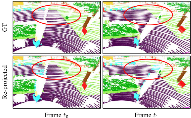
Figure 1. Range-image-based methods suffer from the “many-toone” problem where multiple 3D points with the same angle are mapped to a single range pixel. Marked by the red circles of frame $t_{0}$ , this can cause distant terrain points (purple) to receive erroneous predictions from nearby billboard points (blue) when the range image is re-projected to 3D. Furthermore, occluded points in frame $t_{0}$ become visible in $t_{1}$ , offering an opportunity to refine the predictions.
图 1: 基于距离图像的方法存在"多对一"问题,即具有相同角度的多个3D点会被映射到单个距离像素。如帧 $t_{0}$ 的红圈标记所示,当距离图像重新投影到3D空间时,这会导致远处的地形点(紫色)从附近的广告牌点(蓝色)接收到错误预测。此外,帧 $t_{0}$ 中被遮挡的点在 $t_{1}$ 中变得可见,这为优化预测提供了机会。
However, the range view representation suffers from a boundary-blurring effect [32, 54]. This problem exists mainly because of the limited horizontal and vertical angular resolution: more than one point will be projected to the same range image pixel when these points share the same vertical and horizontal angle. When multiple points share identical vertical and horizontal angles, they are projected onto the same pixel in the range image, giving rise to what is also referred to as the “many-to-one” problem [54]. Considering that the projection computes distant points first and near points later [32], the distant points will be occluded by the near points. Hence, when converting the range image back into 3D coordinates, which is essential for rangeimage-based methods, the farther points receive the same label as the overlapping points that are closer. This leads to inaccuracies in the semantic understanding of the scene.
然而,距离视图表示法存在边界模糊效应 [32, 54]。该问题主要由有限的水平和垂直角分辨率导致:当多个点具有相同的垂直和水平角度时,它们会被投影到距离图像的同一像素上,这种现象也被称为"多对一"问题 [54]。由于投影计算会优先处理远点再处理近点 [32],远点会被近点遮挡。因此,在将距离图像转换回3D坐标(这是基于距离图像方法的关键步骤)时,较远的点会获得与重叠较近点相同的标签,从而导致场景语义理解的不准确性。
Fig. 1 offers an illustration of this problem. Imagine that the LiDAR sensor is situated at the bottom-left of each range image. Close to the sensor, there is a billboard colored blue, and farther away is the terrain, displayed in purple. At time $t_{0}$ , as marked by the red circle, even though the terrain and billboard are physically separate objects, some points on the terrain are incorrectly labeled as part of the billboard. This happens because these points, due to their similar angles relative to the LiDAR sensor, get projected onto the same pixel in the range image. Upon the movement of the car and the consequent change in the sensor’s field of view, we see a different scenario at time $t_{1}$ : the previously mislabeled terrain points are now accurately classified. This improvement is attributed to the fact that their angular positions relative to the LiDAR sensor have changed, allowing them to avoid being hidden or masked by the billboard. This example illustrates how the dynamic movement affects LiDAR-based semantic segmentation and underscores the possibility of developing reliable and adaptable methods to tackle the “many-to-one” issue in this context.
图 1: 展示了该问题的示意图。假设LiDAR传感器位于每个距离图像的左下角。靠近传感器处有一个蓝色的广告牌,远处则是紫色的地形。在$t_{0}$时刻(如红圈标注),尽管地形与广告牌是物理分离的物体,但地形上的部分点被错误标记为广告牌的一部分。这是因为这些点相对于LiDAR传感器的角度相似,导致它们在距离图像中被投影到同一像素上。随着车辆移动及传感器视野变化,$t_{1}$时刻出现了不同情况:先前误标的地形点现已被正确分类。这种改进归因于它们相对于LiDAR传感器的角度位置发生变化,从而避免了被广告牌遮挡或掩盖。该示例说明了动态运动如何影响基于LiDAR的语义分割,并强调了开发可靠、自适应方法来解决此类"多对一"问题的可能性。
We quantitatively assess the effects of this phenomenon on the Semantic KITTI dataset [2, 3]. Under standard conditions, where the range image dimensions are set to 64 and 2048 for height and width, respectively, it is observed that more than $20%$ of the 3D points are occluded within the range image, i.e., more than one point is projected to the same pixel. As detailed in Tab. 3, this results in a substantial degradation of the accuracy if it is not addressed by an additional post-processing step. Therefore, various post-processing approaches like $\mathbf{k}$ -NN [32], CRF [46], or NLA [54] have been proposed. As an example, NLA [54] resorts to assigning the label of the closest non-occluded point to occluded points. Nonetheless, this process necessitates checking each individual point for occlusion, which undermines the inherent efficiency of range-image-based methods. A detailed discussion about these methodologies can be found in Section 2.
我们在Semantic KITTI数据集[2,3]上定量评估了这种现象的影响。在标准条件下(距离图像的高度和宽度分别设置为64和2048),观察到超过20%的3D点在距离图像中被遮挡(即多个点投影到同一像素)。如表3所示,若不通过额外后处理步骤解决该问题,会导致精度显著下降。因此,研究者们提出了多种后处理方法,如k-NN[32]、CRF[46]或NLA[54]。以NLA[54]为例,该方法通过为被遮挡点分配最近未遮挡点的标签来解决该问题。然而,此过程需要逐个检查点的遮挡状态,这会削弱基于距离图像方法固有的高效性。关于这些方法的详细讨论见第2节。
In this work, we propose to incorporate temporal information to address the “many-to-one” challenge for LiDAR semantic segmentation. This is inspired by human visual perception, where temporal information is crucial for understanding object motion and identifying occlusions.
在本工作中,我们提出通过引入时序信息来解决激光雷达 (LiDAR) 语义分割中的"多对一"挑战。这一思路源于人类视觉感知机制——时序信息对于理解物体运动状态和识别遮挡关系至关重要。
This is also observed in LiDAR semantic segmentation, where heavily occluded points can be captured from adjacent range image scans, as shown in Fig. 1. Based on this intuition, we exploit the temporal relations of features in the range map via cross-attention [17, 22, 42]. As for the inference stage, we propose a max-voting-based postprocessing scheme that effectively reuses the predictions of past frames. To this end, we transform the previous scans with predicted semantic class labels into the current ego car coordinate frame and then obtain the final segmentation by aggregating the predictions within the same voxel by maxvoting. In summary, we make the following three contributions:
这也同样适用于激光雷达 (LiDAR) 语义分割任务,如图 1 所示,被严重遮挡的点可以通过相邻距离图像扫描捕获。基于这一观察,我们通过交叉注意力 [17, 22, 42] 利用距离图中特征的时序关系。针对推理阶段,我们提出了一种基于最大投票的后处理方案,可有效复用历史帧的预测结果。具体而言,我们将带有预测语义类别标签的历史扫描数据转换到当前自车坐标系,然后通过最大投票聚合同一体素内的预测结果以获得最终分割。本文的核心贡献可总结为以下三点:
2. RELATED WORK
2. 相关工作
LiDAR semantic segmentation. The LiDAR sensor captures high-fidelity 3D structural information, which can be represented by various formats, i.e., points [34, 35, 40], range view [13, 21, 32, 46, 54], voxels [14, 27, 55], bird’s eye view (BEV) [8], hybrid [24, 36] and multi-modal representations [7, 51, 56]. There are also some works [51, 56] that fuse multi-sensor information. The point and voxel methods are prevailing, but their complexity is $\mathcal{O}(N\cdot d)$ where $N$ is in the order of $10^{5}$ [41]. Thus, most approaches are not suitable for robotics or autonomous driving applications. The BEV method [8] offers a more efficient choice with $\textstyle{\mathcal{O}}({\frac{H\cdot W}{r^{2}}}\cdot d)$ complexity, but the accuracy is subpar [21]. The multi-modal methods require additional resources to process the additional modalities. Among all representations, the range view reflects the LiDAR sampling process and it is much more efficient than other representations with $\textstyle{\mathcal{O}}({\frac{H\cdot W}{r^{2}}}\cdot d)$ complexity. We thus focus on the range-view as representation.
LiDAR语义分割。LiDAR传感器捕获的高保真3D结构信息可通过多种形式表示,包括点云 [34, 35, 40]、距离视图 [13, 21, 32, 46, 54]、体素 [14, 27, 55]、鸟瞰图 (BEV) [8]、混合表示 [24, 36] 以及多模态表征 [7, 51, 56]。另有研究 [51, 56] 融合多传感器信息。点云与体素方法虽主流,但其复杂度为 $\mathcal{O}(N\cdot d)$(其中 $N$ 达 $10^{5}$ 量级 [41]),多数方法不适用于机器人或自动驾驶场景。BEV方法 [8] 以 $\textstyle{\mathcal{O}}({\frac{H\cdot W}{r^{2}}}\cdot d)$ 复杂度提供更高效选择,但精度欠佳 [21]。多模态方法需额外资源处理辅助模态。距离视图直接反映LiDAR采样过程,且以 $\textstyle{\mathcal{O}}({\frac{H\cdot W}{r^{2}}}\cdot d)$ 复杂度显著优于其他表征形式,故本文聚焦距离视图表征。
Multi-frame LiDAR data processing. Multi-frame information plays a crucial role in LiDAR data processing. For example, MOS [12] and MotionS eg 3 D [39] generate residual images from multiple LiDAR frames to explore the sequential information and use it for segmenting moving and static objects. Motivated by these approaches, MetaRangeSeg [45] also uses residual range images for the task of semantic segmentation of LiDAR sequences. It employs a meta-kernel to extract the meta features from the residual images. SeqOT [29] exploits sequential LiDAR frames using yaw-rotation-invariant Overlap Nets [10, 11] and transformer networks [30, 42] to generate a global descriptor for fast place recognition in an end-to-end manner. In addition, SCPNet [48] designs a knowledge distillation strategy between multi-frame LiDAR scans and a single-frame LiDAR scan for semantic scene completion. Recently, Mars3D [25] designed a plug-and-play motion-aware module for multiscan 3D point clouds to classify semantic categories and motion states. Seal [26] proposes a temporal consistency loss to constrain the semantic prediction of super-points from multiple scans. Although the benefit of using multiple scans has been studied, these works address other tasks. Post processing. Although range-view-based LiDAR segmentation methods are computationally efficient, they suffer from boundary blurriness or the “many-to-one” issue [32, 46] as discussed in Sec. 1. To alleviate this issue, most works use a conditional random field (CRF) [46] or $\mathbf{k}$ -NN [32] to smooth the predicted labels. [46] implements the CRF as an end-to-end trainable recurrent neural network to refine the predictions according to the predictions of the neighbors within three iterations. It does not address occluded points explicitly. $\mathbf{k}$ -NN [32] infers the semantics of ambiguous points by jointly considering its k closest neighbours in terms of the absolute range distance. However, finding a balance between under and over-smoothing can be challenging, and it may not be able to handle severe occlusions. Recently, NLA [54] assigns the nearest point’s prediction in a local patch to the occluded point. However, it is required to iterate over each point to verify occlusions. In addition, Range Former [21] addresses this issue by creating sub-clouds from the entire point cloud and inferring labels for each subset. However, partitioning the cloud into subclouds ignores the global information. It can also not easily be applied to existing networks. Some methods [1, 20, 39] propose additional refinement modules for the networks to refine the initial estimate, which increases the runtime. In this work, we propose to tackle this issue by combining past predictions in an efficient max-voting manner. Our method complements existing approaches and can be applied to various networks.
多帧LiDAR数据处理。多帧信息在LiDAR数据处理中起着关键作用。例如,MOS [12] 和 MotionSeg3D [39] 通过多帧LiDAR数据生成残差图像来挖掘时序信息,用于分割运动与静态物体。受此启发,MetaRangeSeg [45] 同样利用残差距离图像完成LiDAR序列语义分割任务,采用元核(meta-kernel)从残差图像中提取元特征。SeqOT [29] 通过偏航旋转不变重叠网络(yaw-rotation-invariant Overlap Nets) [10, 11] 和Transformer网络 [30, 42] 处理连续LiDAR帧,以端到端方式生成全局描述符实现快速场景识别。此外,SCPNet [48] 设计了多帧LiDAR扫描与单帧扫描间的知识蒸馏策略用于语义场景补全。近期,Mars3D [25] 开发了即插即用的多扫描3D点云运动感知模块,可同步分类语义类别与运动状态。Seal [26] 提出时序一致性损失函数来约束多帧扫描中超点(super-points)的语义预测。尽管多帧扫描的优势已被证实,但这些研究均针对其他任务。
后处理。虽然基于距离视图(range-view)的LiDAR分割方法计算高效,但如第1节所述,它们存在边界模糊或"多对一"(many-to-one)问题 [32, 46]。为缓解该问题,多数研究采用条件随机场(CRF) [46] 或 $\mathbf{k}$ -NN [32] 进行预测标签平滑。[46] 将CRF实现为端到端可训练的循环神经网络,通过三轮迭代根据邻域预测优化结果,但未显式处理遮挡点。$\mathbf{k}$ -NN [32] 通过联合考虑k个最近邻的绝对距离来推断模糊点语义,但欠平滑与过平滑的平衡较难把握,且难以处理严重遮挡。近期NLA [54] 将局部块中最近点的预测分配给遮挡点,但需遍历每个点验证遮挡情况。Range Former [21] 通过从完整点云创建子云并为每个子集推断标签来解决该问题,但分割操作会丢失全局信息且难以适配现有网络。部分方法 [1, 20, 39] 提出额外优化模块来改进初始估计,这会增加运行时耗。本文提出通过高效最大投票机制融合历史预测来解决该问题,该方法可兼容现有方案并适用于多种网络。
3. PROPOSED METHOD
3. 研究方法
3.1. Network Overview
3.1. 网络概述
The overview of our proposed network is illustrated in Fig. 2. Our proposed network takes as input a point cloud $P$ comprising $N$ points represented by 3D coordinates $x,y,z$ , and intensity $i$ . The point cloud is projected onto a range image $I$ of size $H\times W\times5$ using a spherical projection technique employed in previous works [32, 46]. Here, $H$ and $W$ represent the height and width of the image, and the last dimension includes coordinates $(x,y,z)$ , range $r=\sqrt{x^{2}+y^{2}+z^{2}}$ , and intensity $i$ . Next, we feed the range image into our backbone model to obtain multi-scale features $F$ with resolutions ${1,1/2,1/4,1/8}$ . We employ a Temporal Cross-Attention (TCA) layer to integrate spatial features from the history frame. The aggregated features are then fed to the segmentation head, which predicts the range-image-based semantic segmentation logits $O$ . For inference, we re-project the 2D semantic segmentation prediction to a 3D point-wise prediction $S$ . Subsequently, we propose a Max-Voting-based Post-processing (MVP) strategy to refine the current prediction $S_{t}$ by aggregating pre- vious predictions. We describe the key components of our network in the following sections.
我们提出的网络概览如图 2 所示。该网络以包含 $N$ 个点的点云 $P$ 作为输入,每个点由 3D 坐标 $(x,y,z)$ 和强度值 $i$ 表示。通过先前工作 [32,46] 采用的球面投影技术,将点云投影为尺寸 $H\times W\times5$ 的距离图像 $I$。其中 $H$ 和 $W$ 表示图像高度和宽度,最后一个维度包含坐标 $(x,y,z)$、距离 $r=\sqrt{x^{2}+y^{2}+z^{2}}$ 以及强度值 $i$。随后将距离图像输入主干网络,获得分辨率分别为 ${1,1/2,1/4,1/8}$ 的多尺度特征 $F$。我们使用时序交叉注意力 (TCA) 层整合历史帧的空间特征,聚合后的特征送入分割头输出基于距离图像的语义分割逻辑值 $O$。推理阶段将 2D 语义分割预测重投影为 3D 点级预测 $S$,并提出基于最大投票的后处理 (MVP) 策略,通过聚合历史预测来优化当前预测结果 $S_{t}$。下文将详细阐述网络的关键组件。
3.2. Temporal cross attention
3.2. 时序交叉注意力 (Temporal cross attention)
Although the range image suffers from the “many-to-one” issue, the occluded points can be captured from adjacent scans. This observation motivates us to incorporate sequential scans into both the training and inference stages. First, we discuss how sequential data can be exploited during the training stage.
尽管距离图像存在“多对一”问题,但被遮挡点可以通过相邻扫描捕获。这一发现促使我们将连续扫描纳入训练和推理阶段。首先讨论如何在训练阶段利用序列数据。
Inspired by the notable information extraction ability of the attention mechanism [42] verified by various other works [22, 31, 44, 49], we use the cross-attention mechanism to model the temporal connection between the previous range feature $F_{t-1}$ and the current range feature $F_{t}$ . The attended value is computed by:
受到注意力机制显著信息提取能力的启发[42],这一点已被多项其他研究[22, 31, 44, 49]所验证,我们采用交叉注意力机制来建模前一时刻范围特征$F_{t-1}$与当前范围特征$F_{t}$之间的时序关联。注意力值通过以下公式计算:
$$
\mathbf{x}{i n}=\operatorname{Attention}(Q,K,V)=\operatorname{Softmax}\left({\frac{Q\cdot K^{\mathsf{T}}}{\sqrt{d_{f}}}}\right)V.
$$
$$
\mathbf{x}{i n}=\operatorname{Attention}(Q,K,V)=\operatorname{Softmax}\left({\frac{Q\cdot K^{\mathsf{T}}}{\sqrt{d_{f}}}}\right)V.
$$
where $Q,K,V$ are obtained by $Q=L i n e a r_{q}(F_{t}) $ , $K=$ $L i n e a r_{k}(F_{t-1})$ , $\begin{array}{r}{V=L i n e a r_{v}(F_{t-1})}\end{array}$ , and $d_{f}$ is the dimension of the range features. We integrate a $3\times3$ convolution into the feed-forward module to encode positional information as in [49] as well as a residual connection [18]. The feed-forward module is defined as follows:
其中 $Q,K,V$ 通过 $Q=Linear_{q}(F_{t})$、$K=Linear_{k}(F_{t-1})$、$V=Linear_{v}(F_{t-1})$ 获得,$d_{f}$ 为范围特征的维度。我们在前馈模块中集成了一个 $3\times3$ 卷积来编码位置信息 [49] ,并采用残差连接 [18] 。前馈模块定义如下:
$$
\begin{array}{r}{\mathbf{x}{o u t}=\mathop{\mathrm{MLP}}(\mathop{\mathrm{GELU}}(\mathop{\mathrm{Conv}}{3\times3}(\mathop{\mathrm{MLP}}(\mathbf{x}{i n}))))+\mathbf{x}_{i n}.}\end{array}
$$
$$
\begin{array}{r}{\mathbf{x}{o u t}=\mathop{\mathrm{MLP}}(\mathop{\mathrm{GELU}}(\mathop{\mathrm{Conv}}{3\times3}(\mathop{\mathrm{MLP}}(\mathbf{x}{i n}))))+\mathbf{x}_{i n}.}\end{array}
$$
The TCA module effectively exploits temporal dependencies in two ways. First, instead of using multiple stacked range features [12], our method extracts temporal information from the previous range features. This not only reduces computational costs but also minimizes the influence of moving objects, which can introduce noise into the data. Secondly, we only utilize the fusion module on the last feature level, which significantly decreases computation complexity. Previous works [17, 22] have shown that the attention at shallower layers is not effective.
TCA模块通过两种方式有效利用时间依赖性。首先,我们的方法不是使用多个堆叠的range特征 [12],而是从先前的range特征中提取时间信息。这不仅降低了计算成本,还减少了移动物体对数据的噪声影响。其次,我们仅在最后一个特征层级上使用融合模块,这显著降低了计算复杂度。先前的研究 [17, 22] 表明,较浅层的注意力机制效果不佳。
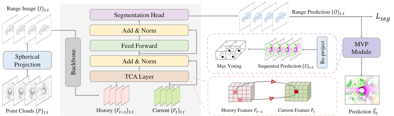
Figure 2. Architecture of TFNet. For a point cloud $P_{t}$ , TFNet projects it onto range images $I_{t}$ . It then uses a segmentation backbone to extract multi-scale features ${F_{t}}{1:l}$ , a Temporal Cross-Attention (TCA) layer to integrate past features ${F_{t-1}}{1:l}$ , and a segmentation head to predict range-image-based logits $O_{t}$ . In inference, it refines the re-projected prediction $S_{t}$ by aggregating the current and past temporal predictions ${S}_{1:t}$ by a Max-Voting-based Post-processing (MVP) strategy.
图 2: TFNet架构。对于点云$P_{t}$,TFNet将其投影到距离图像$I_{t}$上,随后使用分割主干网络提取多尺度特征${F_{t}}{1:l}$,通过时序交叉注意力层(TCA)整合历史特征${F_{t-1}}{1:l}$,并由分割头输出基于距离图像的逻辑值$O_{t}$。在推理阶段,通过基于最大投票的后处理策略(MVP)聚合当前与历史时序预测${S}{1:t}$,优化重投影预测$S_{t}$。
3.3. Max-voting-based post-processing
3.3. 基于最大投票的后处理
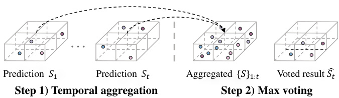
Figure 3. Illustration of the max voting post-processing strategy.
图 3: 最大投票后处理策略示意图。
While temporal cross attention exploits temporal information at the feature level, it does not resolve the “manyto-one” issue during the re-projection process of a rangeimage-based method, which causes occluded far points to inherit the predictions of near points. We thus propose a max-voting-based post-processing (MVP) strategy, which is motivated by the observation that occluded points will be visible in the adjacent scans as shown in Fig. 1. As verified in Tab. 5, MVP is generic and can be added to various networks.
虽然时序交叉注意力在特征层面上利用了时序信息,但并未解决基于距离图像方法在重投影过程中的"多对一"问题,这导致被遮挡的远点会继承近点的预测结果。因此,我们提出了一种基于最大投票的后处理策略 (MVP),其灵感来源于图1所示现象:被遮挡的点在相邻扫描中会变为可见。如表5所示,MVP具有通用性,可应用于各类网络。
Temporal scan alignment. To initiate post-processing, it is essential to align a series of past LiDAR scans $(P_{1},...,P_{t})$ to the viewpoint (i.e., coordinate frame) of $P_{t}$ . The alignment is accomplished by utilizing the estimated relative pose transformations $T_{j-1}^{j}$ between the scans $P_{j-1}$ and $P_{j}$ . These transformation matrices can be acquired from an odometry estimation approach such as $\mathrm{SuMa++}$ [9]. The relative transformations between the scans $(T_{1}^{2},...,T_{t-1}^{t})$ are represented by transformation matrices of $T_{j-1}^{j}\in$ $\mathbb{R}^{4\times4}$ . Further, we denote the $j^{t h}$ scan transformed to the
时间扫描对齐。后处理的第一步是将一系列过去的LiDAR扫描 $(P_{1},...,P_{t})$ 对齐到 $P_{t}$ 的视角(即坐标系)。这一对齐过程通过利用扫描 $P_{j-1}$ 和 $P_{j}$ 之间估计的相对位姿变换 $T_{j-1}^{j}$ 来完成。这些变换矩阵可以通过诸如 $\mathrm{SuMa++}$ [9] 的里程计估计方法获得。扫描之间的相对变换 $(T_{1}^{2},...,T_{t-1}^{t})$ 由 $T_{j-1}^{j}\in$ $\mathbb{R}^{4\times4}$ 的变换矩阵表示。此外,我们将第 $j^{t h}$ 次扫描转换到...
viewpoint of $P_{t}$ by
从 $P_{t}$ 的角度来看
$$
P^{j\to t}={T_{j}^{t}p_{i}}{p_{i}\in P_{j}}\quad\mathrm{with}T_{j}^{t}=\prod_{k=j+1}^{t}T_{k-1}^{k}.
$$
$$
P^{j\to t}={T_{j}^{t}p_{i}}{p_{i}\in P_{j}}\quad\mathrm{with}T_{j}^{t}=\prod_{k=j+1}^{t}T_{k-1}^{k}.
$$
Sparse grid max voting. After applying the transformations, we aggregate the aligned scans. We quantize the aggregated scans into a voxel grid with a fixed resolution $\delta$ . In each grid, we use the max-voting strategy to use the most frequently predicted class label to represent the semantics of all points in the grid. We illustrate this process in Fig. 3 and evaluate the impact of the grid size in Fig. 4. To save computation and memory, we store only the non-empty voxels. This sparse representation allows our method to handle large scenes.
稀疏网格最大投票。应用变换后,我们对齐扫描结果进行聚合。将聚合后的扫描数据量化为固定分辨率$\delta$的体素网格。在每个网格中,采用最大投票策略,使用预测频率最高的类别标签来表示网格内所有点的语义。该过程如图3所示,网格尺寸的影响评估如图4所示。为节省计算和内存资源,我们仅存储非空体素。这种稀疏表示方法使我们的算法能够处理大规模场景。
Sliding window update. We initialize a sliding window $W_{t-L+1:t}$ with the length of $L$ to store the scans and use a FIFO (First In First Out) strategy to update the points falling in each grid. When the LiDAR sensor obtains a new point cloud scan, we add it to this sliding window and remove the oldest scan. We do not use different weights across frames due to the uncertain occlusion problem.
滑动窗口更新。我们初始化一个长度为 $L$ 的滑动窗口 $W_{t-L+1:t}$ 来存储扫描数据,并采用FIFO (First In First Out) 策略更新每个网格内的点。当LiDAR传感器获取新点云扫描时,我们将其加入该滑动窗口并移除最旧的扫描。由于遮挡问题的不确定性,我们未对跨帧数据使用不同权重。
4. EXPERIMENTS
4. 实验
Datasets and evaluation metrics. We evaluate our proposed method on Semantic KITTI [2] and SemanticPOSS [33]. Semantic KITTI [2] is a popular benchmark for LiDAR-based semantic segmentation in driving scenes. It contains 19,130 training frames, 4,071 validation frames, and 20,351 test frames. Each point in the dataset is provided with a semantic label of 19 classes for semantic segmentation. We also evaluate our dataset on the SemanticPOSS [33] dataset, which contains 2988 scenes for training and testing. For evaluation, we follow previous works [13, 21, 46, 54], utilizing the class-wise Intersection over Union (IoU) and mean IoU (mIoU) metrics to evaluate and compare with others.
数据集与评估指标。我们在Semantic KITTI [2]和SemanticPOSS [33]上评估提出的方法。Semantic KITTI [2]是驾驶场景中基于LiDAR的语义分割常用基准,包含19,130帧训练数据、4,071帧验证数据和20,351帧测试数据。数据集中每个点都标注了19类语义分割标签。我们还在SemanticPOSS [33]数据集上进行评估,该数据集包含2,988个训练和测试场景。评估时沿用先前工作[13, 21, 46, 54]的做法,采用逐类交并比(IoU)和平均交并比(mIoU)指标进行性能对比。
Table 1. Comparison with other range-image-based LiDAR segmentation methods with resolution (64, 2048) on Semantic KITTI test set.
表 1: 在 Semantic KITTI 测试集上与其他基于距离图像的 LiDAR 分割方法 (分辨率 64×2048) 的对比。
| 方法 | mean-IoU | car | bicycle | motorcycle | truck | other-vehicle | person | bicyclist | motorcyclist | road | parking | sidewalk | ground | building | fence | vegetation | trunk | terrain | pole | traffic-sign |
|---|---|---|---|---|---|---|---|---|---|---|---|---|---|---|---|---|---|---|---|---|
| MINet [23] | 55.2 | 90.1 | 41.8 | 34.0 | 29.9 | 23.6 | 51.4 | 52.4 | 25.0 | 90.5 | 59.0 | 72.6 | 25.8 | 85.6 | 52.3 | 81.1 | 58.1 | 66.1 | 49.0 | 59.9 |
| FIDNet [54] | 59.5 | 93.9 | 54.7 | 48.9 | 27.6 | 23.9 | 62.3 | 59.8 | 23.7 | 90.6 | 59.1 | 75.8 | 26.7 | 88.9 | 60.5 | 84.5 | 64.4 | 69.0 | 53.3 | 62.8 |
| Meta-RangeSeg [45] | 61.0 | 93.9 | 50.1 | 43.8 | 43.9 | 43.2 | 63.7 | 53.1 | 18.7 | 90.6 | 64.3 | 74.6 | 29.2 | 91.1 | 64.7 | 82.6 | 65.5 | 65.5 | 56.3 | 64.2 |
| KPRNet [20] | 63.1 | 95.5 | 54.1 | 47.9 | 23.6 | 42.6 | 65.9 | 65.0 | 16.5 | 93.2 | 73.9 | 80.6 | 30.2 | 91.7 | 68.4 | 85.7 | 69.8 | 71.2 | 58.7 | 64.1 |
| Lite-HDSeg [38] | 63.8 | 92.3 | 40.0 | 55.4 | 37.7 | 39.6 | 59.2 | 71.6 | 54.1 | 93.0 | 68.2 | 78.3 | 29.3 | 91.5 | 65.0 | 78.2 | 65.8 | 65.1 | 59.5 | 67.7 |
| CENet [13] | 64.7 | 91.9 | 58.6 | 50.3 | 40.6 | 42.3 | 68.9 | 65.9 | 43.5 | 90.3 | 60.9 | 75.1 | 31.5 | 91.0 | 66.2 | 84.5 | 69.7 | 70.0 | 61.5 | 67.6 |
| RangeViT [1] | 64.0 | 95.4 | 55.8 | 43.5 | 29.8 | 42.1 | 63.9 | 58.2 | 38.1 | 93.1 | 70.2 | 80.0 | 32.5 | 92.0 | 69.0 | 85.3 | 70.6 | 71.2 | 60.8 | 64.7 |
| LENet [16] | 64.5 | 93.9 | 57.0 | 51.3 | 44.3 | 44.4 | 66.6 | 64.9 | 36.0 | 91.8 | 68.3 | 76.9 | 30.5 | 91.2 | 66.0 | 83.7 | 68.3 | 67.8 | 58.6 | 63.2 |
| TFNet (Ours) | 66.1 | 94.3 | 60.7 | 58.5 | 38.4 | 48.4 | 74.3 | 72.2 | 35.5 | 90.6 | 68.5 | 75.3 | 29.0 | 91.6 | 67.3 | 83.8 | 71.1 | 67.0 | 60.8 | 68.7 |
Implementation details. While we use CENet [13] as the main baseline method, our method demonstrates robust generalization across various backbones as shown in the following experiments. We train the proposed method using the Stochastic Gradient Descent (SGD) optimizer and set the batch size to 8 and 4 for Semantic KITTI and SemanticPOSS, respectively. We follow the baseline method [13] to supervise the training with a weighted combination of cross-entropy, Lovasz softmax loss [4], and boundary loss [5]. The weights for the loss terms are set to $\beta_{1}=1.0$ , $\beta_{2}=1.5$ , $\beta_{3}=1.0$ , respectively. All the models are trained on GeForce RTX 3090 GPUs. The inference latency is measured using a single GeForce RTX 3090 GPU. The backbone is trained from scratch on all the datasets.
实现细节。虽然我们使用CENet [13]作为主要基线方法,但我们的方法在以下实验中展现出对各种骨干网络的强泛化能力。训练采用随机梯度下降 (Stochastic Gradient Descent, SGD) 优化器,批处理大小在Semantic KITTI和SemanticPOSS数据集上分别设为8和4。我们遵循基线方法[13]的监督策略,采用交叉熵损失、Lovasz softmax损失[4]和边界损失[5]的加权组合,权重系数分别设为 $\beta_{1}=1.0$、$\beta_{2}=1.5$、$\beta_{3}=1.0$。所有模型均在GeForce RTX 3090 GPU上训练,推理延迟测试使用单张同型号GPU完成。骨干网络在所有数据集上均从头开始训练。
4.1. Comparison with state of the art
4.1. 与当前最优技术的对比
Quantitative results on Semantic KITTI. Tab. 1 reports comparisons with representative models on the Seman tic KITTI test set. Our method outperforms all rangeimage-based methods, including CNN-based architectures [13, 23, 54] and Transformer-based architectures [1] in terms of mean IoU. CENet [13] uses test time augmentation to improve the performance. We do not use test time augmentation for a fair comparison with previous methods [23, 32].
语义KITTI定量结果。表1报告了在Semantic KITTI测试集上与代表性模型的对比。我们的方法在平均IoU指标上优于所有基于距离图像的方法,包括基于CNN的架构[13, 23, 54]和基于Transformer的架构[1]。CENet[13]使用了测试时增强(test time augmentation)来提升性能。为与先前方法[23, 32]公平对比,我们未采用测试时增强。
Tab. 1 presents a comprehensive comparison of the proposed TFNet method against several range-image-based LiDAR segmentation models on the Semantic KITTI test set. Specifically, TFNet excels in segmenting cars, bicycles, motorcycles, and pedestrians, showing significant improvements in IoU values over other methods. It registers particularly high IoU scores for bicycles $(60.7%)$ , motorcycles $(58.5%)$ , and persons $(74.3%)$ . Despite not always securing the top position in every class, TFNet consistently delivers strong results, especially in small and medium-sized object classes. TFNet falls slightly behind in the pole and traffic-sign categories, where it records IoU scores lower than some methods like CENet [13] and KPRNet [20]. Nevertheless, its ability to maintain balanced and above-average performance across most classes contributes to its overall leadership in mean-IoU.
表 1 展示了所提出的 TFNet 方法与几种基于距离图像的 LiDAR 分割模型在 Semantic KITTI 测试集上的综合对比。具体而言,TFNet 在汽车、自行车、摩托车和行人分割方面表现优异,其 IoU 值相比其他方法有显著提升。尤其在自行车 $(60.7%)$、摩托车 $(58.5%)$ 和行人 $(74.3%)$ 类别上获得了极高的 IoU 分数。尽管 TFNet 并非在所有类别中都位居第一,但它在中小型物体类别上始终表现强劲。TFNet 在电线杆和交通标志类别上稍显逊色,其 IoU 分数低于 CENet [13] 和 KPRNet [20] 等方法。然而,它在大多数类别中保持均衡且高于平均水平的性能,使其在平均 IoU 指标上总体领先。
Table 2. Evaluation results on the Semantic POS S test set.
表 2: Semantic POS S 测试集上的评估结果
| [46] .Seg | Sq.SegV2 [47] | RangeNet [32] | [23] MINet | [54] FIDNet | [13] CENet | TFNet (Ours) | |
|---|---|---|---|---|---|---|---|
| person | 6.8 | 43.9 | 57.3 | 62.4 | 72.2 | 75.5 | 72.4 |
| rider | 0.6 | 7.1 | 4.6 | 12.1 | 23.1 | 22.0 | 20.5 |
| car | 6.7 | 47.9 | 35.0 | 63.8 | 72.7 | 77.6 | 77.7 |
| truck | 4.0 | 18.4 | 14.1 | 22.3 | 23.0 | 25.3 | 24.8 |
| plants | 2.5 | 40.9 | 58.3 | 68.6 | 68.0 | 72.2 | 71.6 |
| traffic-sign | 9.1 | 4.8 | 3.9 | 16.7 | 22.2 | 18.2 | 29.1 |
| pole | 1.3 | 2.8 | 6.9 | 30.1 | 28.6 | 31.5 | 37.8 |
| trashcan | 0.4 | 7.4 | 24.1 | 28.9 | 16.3 | 48.1 | 46.3 |
| building | 37.1 | 57.5 | 66.1 | 75.1 | 73.1 | 76.3 | 79.9 |
| cone/stone | 0.2 | 0.6 | 6.6 | 58.6 | 34.0 | 27.7 | 34.5 |
| fence | 8.4 | 12.0 | 23.4 | 32.2 | 40.9 | 47.7 | 47.3 |
| bike | 18.5 | 35.3 | 28.6 | 44.9 | 50.3 | 51.4 | 53.9 |
| ground | 72.1 | 71.3 | 73.5 | 76.3 | 79.1 | 80.3 | 78.4 |
| mean-IoU | 12.9 | 26.9 | 30.9 | 43.2 | 46.4 | 50.3 | 51.9 |
Quantitative results on Semantic POS S. We present a quantitative evaluation of our TFNet method against several range-image-based LiDAR segmentation models on the Semantic POS S test set [33] in Tab. 2. Our method achieves the highest mean Intersection-over-Union (mIoU) among all listed methods, indicating overall better segmentation accuracy. Notably, TFNet excels in detecting smaller objects. It significantly surpasses CENet in segmenting traffic signs and poles, improving the IoU score by 6.9 percentage points and 6.3 percentage points, respectively. Furthermore, TFNet performs competitively in identifying cone/stone, achieving the second-best IoU score, closely following MINet’s performance. Moreover, TFNet ranks second in multiple categories such as rider, plants, fence, and bike, demonstrating its strong general iz ability across diverse object classes.
语义POS S定量结果。我们在表2中展示了TFNet方法与几种基于距离图像的LiDAR分割模型在语义POS S测试集[33]上的定量评估结果。我们的方法在所有列出的方法中取得了最高的平均交并比(mIoU),表明其整体分割精度更优。值得注意的是,TFNet在检测较小物体方面表现突出:其分割交通标志和立柱的IoU分数分别比CENet高出6.9个百分点和6.3个百分点。此外,TFNet在识别锥形物/石块方面表现优异,以仅次于MINet的成绩获得第二高的IoU分数。该模型还在骑行者、植物、围栏和自行车等多个类别中排名第二,展现了其在不同物体类别间的强大泛化能力。
Table 3. Comparison with different post-processing methods. Our MVP method is significantly better.
表 3: 不同后处理方法的对比。我们的 MVP 方法显著优于其他方法。
| | mean-IoU | 其他车辆 摩托车手 其他地面 摩托车 骑行者 停车区 人行道 建筑物 |
| | 自行车 汽车 |
| w/oMVP 60.4 CRF [46] 58.2 (-2.2) | |
| PointRefine [39] 59.2 (-1.2) | 84.5 43.7 53.7 76.3 48.6 68.3 70.6 7.5 285.7 12.4 94.5 42.7 80.8 10.6 87.3 54.6 85.9 66.0 72.2 63.4 49.8 |
| NLA [54] 64.4 (+4.0) | 92.0 47.5 66.8 79.0 55.9 76.2 |
| k-NN [32] | 91.4 50.7 766.9 81.2 54.9 76.8 85.1 0.9 694.5 41.6 80.9 0.9 588.5 55.6 86.2 |
| 64.5 (+4.1) MVP (Ours) 66.5 (+6.1) | |
4.2. Ablation Analysis
4.2. 消融分析
Effect of the temporal post-processing. Tab. 3 compares the proposed post-processing method with other postprocessing approaches on the Semantic KITTI validation set. Using a CRF for post-processing has been used by Seque eze Seg v 2 [47]. We train the network with CRF from scratch using the same training pipeline as our method. The $\mathbf{k}$ -Nearest Neighbor (k-NN) method [32] is the most popular post-processing method. It is widely used in Lite-HDseg [38], Se que eze Seg v 3 [50], CENet [13], SalsaNext [15], and MiNet [23]. The Nearest Label Assignment (NLA) post-processing is used by FIDNet [54]. It iterates over each point to check if a point is occluded or not. We use the source code from the corresponding methods. For the Point Refine module proposed in MotionSeg3D [39], we follow its implementation. We use SPVCNN [27] as the Point Refine module and use the features before the classification layer as the input to the Point Refine module. We then fine-tune the network with the Point Refine module in a second stage with a 0.001 learning rate for ten epochs. The results show the “many-to-one” issue harms the performance heavily. Without our proposed post-processing (‘w/o MVP’), the mean IoU is 6.1 lower. That CRF can actually decrease the mean IoU has also been shown in [32]. While NLA and $\mathbf{k}$ -NN improve the results, the best mean IoU is achieved by our approach.
时间后处理的效果。表3比较了所提出的后处理方法与其他后处理方法在Semantic KITTI验证集上的表现。SequeezeSeg v2 [47]曾使用CRF进行后处理。我们采用与本文方法相同的训练流程,从头开始训练带CRF的网络。k近邻(k-NN)方法[32]是最流行的后处理方法,被广泛应用于Lite-HDseg [38]、SqueezeSeg v3 [50]、CENet [13]、SalsaNext [15]和MiNet [23]中。FIDNet [54]使用了最近邻标签分配(NLA)后处理方法,该方法会遍历每个点以检查是否被遮挡。我们使用各方法的源代码实现。对于MotionSeg3D [39]提出的点细化模块,我们遵循其实现方式:采用SPVCNN [27]作为点细化模块,并使用分类层前的特征作为输入,随后以0.001学习率对带点细化模块的网络进行10个epoch的二阶段微调。结果表明"多对一"问题严重影响性能,未使用本文后处理方法('w/o MVP')时平均IoU下降6.1。[32]也证实CRF会降低平均IoU。虽然NLA和k-NN能改善结果,但本文方法取得了最佳平均IoU。
Table 4. Comparison with other temporal fusion methods.
表 4: 与其他时序融合方法的对比
| 融合策略 | mIoU |
|---|---|
| 无TCA | 66.9 |
| TMA模块 [43] | 67.8 (+0.9) |
| 残差图像 [45] | 61.4 (-5.5) |
| 逐元素相加 [25] | 67.6 (+0.7) |
| 通道拼接 [52] | 68.0 (+1.1) |
| TCA模块 (本文) | 68.1 (+1.2) |
Effect of different fusion strategy. In Tab. 4, we replace the proposed temporal fusion layer with other strategies. Mars3D [25] adopts element-wise summation to aggregate temporal multi-scan point cloud embeddings and produce enhanced features. The temporal memory attention (TMA) module [43] validates its effectiveness on the video semantic segmentation task. BEVFormer v2 [52] uses a feature warp and concatenation strategy to incorporate temporal information and shows its effectiveness on the LiDAR detection task. We follow its implementation, which concatenates previous BEV features with the current BEV feature along the channel dimension and employs residual blocks for dimensionality reduction. We transform the scans to the same ego-car coordinates to implement the accurate alignment between temporal scans. For the LiDAR semantic segmentation task, Meta-RangeSeg [45] proposes to use three previous residual images as input and a meta-kernel module to incorporate temporal information. We follow its implementation and add to the five-channel input (x,y,z,r,i) three channels for the three residual images and a channel for the mask, which indicates whether the pixel is a projected 3D point or not. The residual images are calculated by first transforming the point clouds of previous frames into the coordinates of the current frame and then calculating the absolute differences between the range values of the current scan and the transformed one with normalization. A metakernel is followed to capture the spatial and temporal information. For a fair comparison, we keep the encoder and decoder of our architecture. We report the projection-based mIoU here because the loss function is applied directly to the range image. All strategies are trained with the same setting and pipeline. The results in Tab. 4 show that our temporal fusion approach performs best.
不同融合策略的效果。在表4中,我们将提出的时序融合层替换为其他策略。Mars3D [25] 采用逐元素求和来聚合时序多扫描点云嵌入并生成增强特征。时序记忆注意力 (TMA) 模块 [43] 在视频语义分割任务中验证了其有效性。BEVFormer v2 [52] 使用特征变形和拼接策略来融合时序信息,并在LiDAR检测任务中展示了其效果。我们遵循其实现方式,将先前的BEV特征与当前BEV特征沿通道维度拼接,并采用残差块进行降维。我们将扫描转换到相同的自车坐标系以实现时序扫描间的精确对齐。对于LiDAR语义分割任务,Meta-RangeSeg [45] 提出使用三个先前的残差图像作为输入,并通过元核模块融合时序信息。我们遵循其实现方式,在五通道输入 (x,y,z,r,i) 基础上增加了三个残差图像通道和一个掩码通道(用于标识像素是否为投影的3D点)。残差图像的计算方式是:先将先前帧的点云转换到当前帧坐标系,然后计算当前扫描与转换后扫描的距离值绝对差并进行归一化。随后通过元核捕获时空信息。为公平比较,我们保留了架构中的编码器和解码器。此处报告基于投影的mIoU,因为损失函数直接作用于距离图像。所有策略均采用相同的训练设置和流程。表4结果显示,我们的时序融合方法性能最佳。
Table 5. Performance on other range-image-based methods.
表 5: 基于范围图像的其他方法性能表现
| Backbone | Post-processing | k-NN [32] | MVP (Ours) |
|---|---|---|---|
| FIDNet [54] | 55.4 | 58.6 (+3.2) | 61.5 (+6.1) |
| Meta-RangeSeg [45] | 56.6 | 60.3 (+3.7) | 63.1 (+6.5) |
| CENet [13] | 58.8 | 62.6 (+3.8) | 64.7 (+5.9) |
4.3. Generalization Ability
4.3. 泛化能力
Tab. 5 presents the effectiveness of the proposed maxvoting-based post-processing (MVP) technique when integrated with three different range-image-based semantic segmentation methods, specifically FIDNet [54], MetaRangeSeg [45], and CENet [13]. Unlike results reported in Tab. 1, which reflect performances on the test set, this table displays the outcomes obtained on the validation set using publicly available pre-trained models with and without post-processing. For each backbone model, the table compares three post-processing scenarios: no postprocessing (denoted as ‘-’), application of the k-NN method from [32], and our proposed MVP. Each row shows the mean Intersection-over-Union (IoU) scores resulting from these treatments.
表 5 展示了基于最大投票的后处理 (MVP) 技术与三种不同基于距离图像的语义分割方法 (具体为 FIDNet [54]、MetaRangeSeg [45] 和 CENet [13]) 结合时的有效性。与表 1 中反映测试集性能的结果不同,本表展示了使用公开预训练模型在验证集上应用后处理前后的结果。针对每个骨干模型,表格比较了三种后处理场景:无后处理 (标记为"-")、应用 [32] 中的 k-NN 方法,以及我们提出的 MVP。每行显示了这些处理方法产生的平均交并比 (IoU) 分数。
It is evident from the table that employing the MVP consistently leads to notable improvements over the baseline scores (without any post-processing) and often surpasses the performance of $\mathrm{k\Omega}$ -NN post-processing. For instance, MVP increases the IoU score of FIDNet by 6.1 points compared to its base result, demonstrating superior refinement capabilities. Similarly, the IoU scores of Meta-RangeSeg and CENet also witness considerable boosts with the use of MVP, affirming its broad applicability and positive impact on various range-image-based semantic segmentation models.
从表中可以明显看出,采用MVP始终能显著超越基线分数(未经任何后处理),并经常优于$\mathrm{k\Omega}$-NN后处理的性能。例如,MVP将FIDNet的IoU分数相比基础结果提升了6.1分,展现出卓越的优化能力。同样地,Meta-RangeSeg和CENet的IoU分数在使用MVP后也获得显著提升,证实了该方法对各类基于距离图像的语义分割模型具有广泛适用性和积极影响。

Figure 4. Effect of window size and grid size resolution.
图 4: 窗口尺寸与网格分辨率的影响。
4.4. Further Analysis
4.4. 进一步分析
Effect of frame numbers. In Fig. 4 (a), we delve into the effect of frame numbers, investigating the optimal length L of the sliding window used for temporal updates. This parameter determines the number of consecutive LiDAR frames that are combined to exploit temporal coherence in the scene as described in Sec. 3.3. Our analysis reveals that setting L to 10 frames achieves a desirable balance between capturing sufficient temporal context and avoiding excessive computational load or memory requirements. This optimal choice also enables the model to effectively leverage temporal dependencies while maintaining real-time performance and reducing potential noise introduced by distant past or future frames.
帧数的影响。在图 4 (a) 中,我们深入研究了帧数的影响,探讨了用于时间更新的滑动窗口最佳长度 L。该参数决定了结合多少连续 LiDAR 帧以利用场景中的时间连贯性,如第 3.3 节所述。我们的分析表明,将 L 设置为 10 帧能在捕捉足够时间上下文与避免过高计算负载或内存需求之间取得理想平衡。这一最优选择还能让模型有效利用时间依赖性,同时保持实时性能并减少由遥远过去或未来帧引入的潜在噪声。
Effect of grid size resolution. As mentioned in Sec. 3.3, we convert the accumulated LiDAR scans into a voxel grid format with a fixed resolution. It is crucial to select an appropriate resolution because the fundamental assumption is that all points enclosed within a voxel belong to the same semantic category. Overestimating the voxel size can undermine this assumption, whereas selecting a resolution that is too fine can introduce noise into the estimates due to the inclusion of small-scale variations. To investigate the consequences of different voxel sizes, we perform an evaluation showcased in Fig. 4(b). The results clearly demonstrate that a voxel resolution of 0.10 meters yields the best semantic segmentation outcome. This finding underscores the significance of carefully tuning the grid size resolution to ensure that it neither oversimplifies nor over complicates the represent ation of the point cloud data, thereby preserving the integrity and accuracy of the semantic segmentation task.
网格尺寸分辨率的影响。如第3.3节所述,我们将累积的LiDAR扫描数据转换为固定分辨率的体素网格格式。选择合适的分辨率至关重要,因为基本假设是体素内包含的所有点都属于同一语义类别。过高估计体素尺寸会破坏这一假设,而选择过细的分辨率则会因包含小尺度变化而给估计带来噪声。为探究不同体素尺寸的影响,我们在图4(b)中展示了评估结果。结果表明,0.10米的体素分辨率能产生最佳语义分割效果。这一发现强调了精细调整网格尺寸分辨率的重要性,以确保点云数据的表示既不过于简化也不过度复杂,从而保持语义分割任务的完整性和准确性。
Inference time comparison. We visualize popular methods’ inference time and mIoU in Fig. 6. The results show that range-image-based methods are faster than point, polar, or hybrid methods. We measured the inference time of all the methods on the same hardware with a GeForce RTX 3090 GPU for a fair comparison.
推理时间对比。我们在图6中展示了各主流方法的推理时间和mIoU指标。结果表明,基于距离图像(range-image)的方法比点云、极坐标或混合方法更快。为确保公平比较,所有方法的推理时间均在配备GeForce RTX 3090 GPU的相同硬件环境下测量。
Qualitative evaluation. The “many-to-one” issue becomes apparent in the absence of any post-processing technique, as depicted in Fig. 5(a). Here, we observe that points belonging to the tree trunk inadvertently adopt the predictions intended for nearby points from the traffic sign and vegetation classes. This occurs because these points, despite being distinct physical entities, are projected onto the same range pixel in the LiDAR data. In Fig. 5(b), we illustrate the performance of the commonly-employed k-NN method [32]. While it does refine the initial predictions to some extent, it struggles to rectify false classifications when larger regions are occluded. This limitation highlights the inability of certain post-processing methods to handle complex scenarios where multiple points project to the same pixel. On the contrary, our proposed method effectively tackles this problem, as shown in Fig. 5(c). By incorporating temporal information across multiple scans, our approach consistently maintains the correct predictions for the tree trunk, even when the current scan is affected by the “many-to-one” issue. This capability showcases the merit of introducing temporal context in the post-processing phase, as it allows our method to discern and rectify errors caused by occlusions and projection ambiguities in LiDAR data. Thus, our solution demonstrates improved robustness in handling the “many-to-one” problem, illustrating the potential gains achieved by leveraging temporal coherence in LiDAR semantic segmentation.
定性评估。如图5(a)所示,未采用任何后处理技术时,"多对一"问题尤为明显。可以观察到,树干上的点会错误地采纳交通标志和植被类别的邻近点预测结果。这是因为这些点虽属于不同物理实体,却在激光雷达(LiDAR)数据中被投影到同一个距离像素上。图5(b)展示了常用k-NN方法[32]的表现,虽然该方法对初始预测有所改善,但在处理大面积遮挡导致的错误分类时仍显不足,这暴露了某些后处理方法难以应对多点投影至同一像素的复杂场景。相比之下,我们提出的方法有效解决了该问题(见图5(c)),通过融合多帧扫描的时间信息,即使当前帧存在"多对一"问题,仍能持续保持对树干的正确预测。这种能力凸显了在后处理阶段引入时序上下文的价值,使我们的方法能够识别并修正激光雷达数据中由遮挡和投影歧义导致的错误。因此,我们的方案在处理"多对一"问题时展现出更强的鲁棒性,证明了利用时序一致性可为激光雷达语义分割带来显著提升。

Figure 5. Qualitative analysis of the post-processing scheme. (a) The “many-to-one” issue is evident without post-processing, e.g., the trunk is partially segmented as traffic sign and vegetation as they project onto the same range pixel (row 2). (b) $\mathbf{k}$ -NN [32] smooths the semantic labels locally, but it cannot resolve ambiguities by objects that are close or prediction errors. (c) Our method exploits temporal information to resolve false predictions (row 1) or ambiguities due to occlusions (row 2). Best viewed in color.
图 5: 后处理方案的定性分析。(a) 未经后处理时存在明显的"多对一"问题,例如树干被部分分割为交通标志和植被,因为它们投影到同一距离像素上(第2行)。(b) $\mathbf{k}$ -NN [32] 在局部平滑语义标签,但无法解决近距离物体或预测错误导致的歧义。(c) 我们的方法利用时序信息纠正错误预测(第1行)或遮挡导致的歧义(第2行)。建议彩色查看。

Figure 6. mIoU vs. runtime on Semantic KITTI. Our method balances mIoU and inference time better than other state-of-the-art methods. Best viewed in color.
图 6: Semantic KITTI数据集上mIoU与运行时间的关系。我们的方法在mIoU和推理时间之间取得了比其他最先进方法更好的平衡。建议彩色查看。
5. CONCLUSION
5. 结论
In this paper, we quantitatively and qualitatively analyzed the boundary blurriness, which is also called “many-to-one” problem, for range-image-based LiDAR segmentation, and introduced a novel solution named TFNet to tackle it. Our approach involves leveraging temporal information through the introduction of temporal fusion layers during the training process and a sequential max voting strategy during inference. The experiments on two benchmarks demonstrate the advantages of the proposed strategy. In particular, the incorporation of temporal data allows TFNet to maintain robust performance in environments with substantial occlusions, while still maintaining real-time performance. Additionally, we conducted comprehensive ablation studies to validate the design, as well as the broader adaptability of the proposed post-processing to other neural network architectures.
本文通过定量和定性分析,研究了基于距离图像的激光雷达分割中边界模糊性(也称为"多对一"问题),并提出名为TFNet的创新解决方案。该方法通过在训练过程中引入时序融合层,以及在推理阶段采用序列最大投票策略来利用时序信息。在两个基准测试上的实验验证了所提策略的优势:时序数据的融合使TFNet能在严重遮挡环境中保持稳健性能,同时维持实时处理能力。此外,我们通过全面的消融实验验证了网络设计,并证明所提后处理方法对其他神经网络架构具有广泛适应性。
Acknowledgment This work was supported by the Meituan Academy of Robotics Shenzhen. The views and conclusions contained herein are those of the authors and should not be interpreted as necessarily representing the official policies or endorsements, either expressed or implied, of Meituan. Shijie Li was supported by the Deutsche For s chung s gemeinschaft (DFG, German Research Foundation) GA1927/5-2 (FOR 2535 Anticipating Human Behav- ior).