On the Difficulty of Evaluating Baselines A Study on Recommend er Systems
论基线评估的难度:推荐系统研究
Abstract
摘要
Numerical evaluations with comparisons to baselines play a central role when judging research in recommend er systems. In this paper, we show that running baselines properly is difficult. We demonstrate this issue on two extensively studied datasets. First, we show that results for baselines that have been used in numerous publications over the past five years for the Movielens 10M benchmark are suboptimal. With a careful setup of a vanilla matrix factorization baseline, we are not only able to improve upon the reported results for this baseline but even outperform the reported results of any newly proposed method. Secondly, we recap the tremendous effort that was required by the community to obtain high quality results for simple methods on the Netflix Prize. Our results indicate that empirical findings in research papers are questionable unless they were obtained on standardized benchmarks where baselines have been tuned extensively by the research community.
在推荐系统研究中,与基线方法的数值对比评估具有核心意义。本文揭示了正确运行基线方法的复杂性,并通过两个经典数据集进行论证。首先,我们发现过去五年间Movielens 10M基准测试中广泛使用的基线结果存在优化不足。通过精细配置标准矩阵分解(Matrix Factorization)基线,我们不仅改进了文献中该基线的报告结果,甚至超越了所有新提出方法的报告性能。其次,我们回顾了研究社区为在Netflix Prize数据集上获得简单方法的高质量结果所付出的巨大努力。这些结果表明,除非研究结果建立在经过学界充分调优的标准化基准上,否则论文中的实证结论可能存在疑问。
1 Introduction
1 引言
In the field of recommendation systems, numerical evaluations play a central role for judging research. Newly published methods are expected to be compared to baselines, i.e., well-known approaches, in order to measure the improvements over prior work. The best practices require reproducible experiments on several datasets with a clearly described evaluation protocol, baselines tuned by hyperparameter search, and testing for statistical significance of the result. Findings from such experiments are considered reliable. In this work, we question this practice and show that running baselines properly is difficult.
在推荐系统领域,数值评估是评判研究的核心标准。新发布的方法需要与基线方法(即知名方法)进行对比,以衡量其对先前工作的改进。最佳实践要求:在多个数据集上进行可复现的实验、明确描述评估方案、通过超参数搜索调优基线方法,并检验结果的统计显著性。这类实验得出的结论通常被认为是可靠的。本研究对这一实践提出质疑,并证明正确运行基线方法具有相当难度。
We highlight this issue on the extensively studied Movielens 10M (ML10M) benchmark [11]. Over the past five years, numerous new recommendation algorithms have been published in prestigious conferences such as ICML [17, 21, 36],
我们在广泛研究的Movielens 10M (ML10M)基准测试[11]中强调了这一问题。过去五年间,众多新推荐算法发表在ICML[17, 21, 36]等顶级会议上,
NeurIPS [18], WWW [31, 19], SIGIR [5], or AAAI [20, 4] reporting large improvements over baseline methods. However, we show that with a careful setup of a vanilla matrix factorization baseline, we are not only able to outperform the reported results for this baseline but even the reported results of any newly proposed method. Our findings question the empirical conclusions drawn from five years of work on this benchmark. This is worrisome because the ML10M benchmark follows the best practices of reliable experiments. Even more, if results on a well studied benchmark such as ML10M are misleading, typical one-off evaluations are more prone to producing unreliable results. Our explanation for the failure of providing reliable results is that the difficulty of running baselines is widely ignored in our community. This difficulty of properly running machine learning methods could be observed on the Netflix Prize [2] as well. Section 2.2 recaps the tremendous community effort that was required for achieving high quality results for vanilla matrix factorization. Reported results for this simple method varied substantially but eventually the community arrived at well-calibrated numbers. The Netflix Prize also highlights the benefits of rigorous experiments: the findings stand the test of time and, as this paper shows, the best performing methods of the Netflix Prize also work best on ML10M.
NeurIPS [18]、WWW [31, 19]、SIGIR [5] 或 AAAI [20, 4] 报告了相比基线方法的显著改进。然而,我们表明,通过精心设置一个普通的矩阵分解 (matrix factorization) 基线,我们不仅能够超越该基线的报告结果,甚至还能超越任何新提出方法的报告结果。我们的发现质疑了五年来在该基准上得出的实证结论。这令人担忧,因为 ML10M 基准遵循了可靠实验的最佳实践。更甚的是,如果像 ML10M 这样经过充分研究的基准结果存在误导性,那么典型的一次性评估更容易产生不可靠的结果。我们对未能提供可靠结果的解释是,社区广泛忽视了运行基线的难度。这种正确运行机器学习方法的困难在 Netflix Prize [2] 中也能观察到。第 2.2 节回顾了实现高质量普通矩阵分解结果所需的巨大社区努力。这一简单方法的报告结果差异很大,但最终社区得出了经过良好校准的数字。Netflix Prize 也凸显了严格实验的好处:这些发现经受住了时间的考验,并且如本文所示,Netflix Prize 中表现最佳的方法在 ML10M 上也表现最好。
Recognizing the difficulty of running baselines has implications both for conducting experiments and for drawing conclusions from them. The common practice of one-off evaluations where authors run several baselines on a few datasets is prone to suboptimal results and conclusions should be taken with care. Instead, high confidence experiments require standardized benchmarks where baselines have been tuned extensively by the community. Finally, while our work focuses exclusively on evaluations, we want to emphasize that empirical comparisons using fixed metrics are not the only way to judge work. For example, despite comparing to sub-optimal baselines on the ML10M benchmark, recent research has produced many useful techniques, such as local low rank structures [17], mixtures of matrix approximation [18], and auto encoders [31].
认识到运行基线模型的困难对实验开展和结论推导都有重要影响。当前常见的做法是作者在少量数据集上对若干基线模型进行一次性评估,这种做法容易导致次优结果,相关结论需谨慎对待。相比之下,高可信度实验需要建立在经过社区广泛调优的标准化基准之上。最后需要强调的是,虽然本文仅聚焦于评估环节,但基于固定指标的实证比较并非评判工作的唯一方式。例如在ML10M基准测试中,尽管存在基线模型未充分优化的问题,近期研究仍催生了局部低秩结构[17]、矩阵近似混合[18]和自动编码器[31]等多项实用技术。
2 Observations
2 观察结果
In this section, we first examine the commonly used Movielens 10M benchmark for rating prediction algorithms [17, 31, 5, 36, 32, 3, 21, 4, 18, 19]. We show that by carefully setting up well known methods, we can largely outperform previously reported results. The surprising results include (1) Bayesian MF [29, 8] which was reported by previous authors to be one of the poorest performing methods, can outperform any result reported so far on this benchmark including all of the recently proposed algorithms. (2) Well known enhancements, proposed a decade ago for the Netflix Prize, such as SVD ${++}$ [12] or timeSVD++ [14], can further improve the quality substantially.
在本节中,我们首先研究了常用于评分预测算法的Movielens 10M基准测试[17, 31, 5, 36, 32, 3, 21, 4, 18, 19]。研究表明,通过精心设置已知方法,我们可以大幅超越先前报道的结果。令人惊讶的发现包括:(1) 贝叶斯矩阵分解(Bayesian MF)[29, 8]曾被前人报道为性能最差的方法之一,却能超越该基准测试中所有已报道结果,包括近期提出的各种算法。(2) 十年前为Netflix Prize提出的知名改进方法,如SVD${++}$[12]或timeSVD++[14],仍能显著提升预测质量。
Secondly, we compare these findings to the well documented evolution of results on the Netflix Prize. Also on the Netflix Prize, we observe that setting up methods is challenging. For example, results reported for matrix factorization vary considerably over different publications [9, 16, 22, 10, 24, 29, 25, 1, 37]. However, the Netflix Prize encouraged tweaking and reporting better runs of the same method, so over the long run, the results were well calibrated.
其次,我们将这些发现与Netflix Prize上记录翔实的结果演变进行对比。在Netflix Prize上同样观察到,方法建立具有挑战性。例如,不同文献中报告的矩阵分解(matrix factorization)结果差异显著 [9, 16, 22, 10, 24, 29, 25, 1, 37]。不过Netflix Prize鼓励对同一方法进行调优并报告更优结果,因此长期来看,这些结果得到了良好校准。

Figure 1: Progress on rating prediction measured on the Movielens 10M benchmark. Results marked as blue crosses were reported by the corresponding inventors. Results marked as black triangles were run as baselines by authors of newly invented methods. Results are from [17, 31, 5, 36, 32, 3, 21, 4, 18, 19]. See Table 1 for details.
图 1: Movielens 10M基准测试中评分预测的进展。蓝色叉号标记的结果由相应发明者报告,黑色三角形标记的结果是新方法作者作为基线运行的。结果来自 [17, 31, 5, 36, 32, 3, 21, 4, 18, 19]。详情见表 1。
2.1 Movielens
2.1 Movielens
Measuring Root Mean Square Error (RMSE) on a global random 90:10 split of Movielens 10M is a common benchmark for evaluating rating prediction methods [17, 31, 5, 36, 32, 3, 21, 4, 18]. Figure 1 shows the progress reported over the past 5 years on this benchmark. All newly proposed methods clearly outperform the earlier baselines such as matrix factorization or Boltzman machines [30] (RBM). Both SGD (RSVD, Biased MF) and Bayesian versions (BPMF) of matrix factorization have been found to perform poorly. The figure indicates a steady progress, by improving the state-of-the art in rating prediction considerably. Many results include also standard deviations to show that the results are statistically significant, e.g., [32, 18].
在Movielens 10M数据集上采用全局随机90:10分割测量均方根误差(RMSE)是评估评分预测方法的常用基准[17, 31, 5, 36, 32, 3, 21, 4, 18]。图1展示了过去5年该基准测试的进展报告。所有新提出的方法都明显优于早期基线方法,如矩阵分解或玻尔兹曼机30。无论是随机梯度下降版本(RSVD, Biased MF)还是贝叶斯版本(BPMF)的矩阵分解方法,表现都较差。该图表表明通过显著提升评分预测的最新技术水平,研究取得了稳步进展。许多结果还包含了标准差以证明结果具有统计显著性,例如[32, 18]。
2.1.1 A Closer Look at Baselines
2.1.1 基线方法深入解析
The reported results for Biased MF, RSVD, ALS-WR, and BPMF indicate some issues.
Biased MF、RSVD、ALS-WR和BPMF的报告结果显示出一些问题。
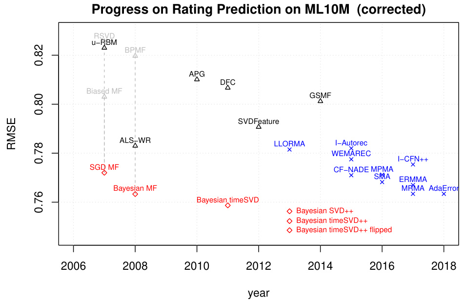
Figure 2: Rerunning baselines for Bayesian MF, and adding popular methods such as Bayesian versions of $\mathrm{SVD++}$ , timeSVD $^{++}$ , timeSVD1. Bayesian MF ( $=$ BPMF) and SGD MF ( $=$ RSVD, Biased MF) can achieve much better results than previously reported. With a proper setup, well known methods can outperform any recently proposed method on this benchmark.
图 2: 重新运行贝叶斯矩阵分解 (Bayesian MF) 的基线,并加入流行方法如贝叶斯版本的 $\mathrm{SVD++}$、timeSVD$^{++}$、timeSVD1。贝叶斯矩阵分解 ($=$ BPMF) 和随机梯度下降矩阵分解 ($=$ RSVD, Biased MF) 能取得比先前报道更好的结果。通过适当设置,这些知名方法在该基准测试中可以超越任何近期提出的方法。
2.1.2 Rerunning Baselines
2.1.2 重新运行基线
We reran the baselines and a different picture emerged (see Figure 2 and Table 1). More details about the experiments can be found in the Appendix.
我们重新运行了基线模型,结果呈现出不同的情况 (参见图 2 和表 1)。实验的更多细节可在附录中找到。
Matrix Factorization First, we ran a matrix factorization model learned by an SGD algorithm (similar to RSVD and Biased MF). SGD-MF achieved an RMSE of 0.7720 for a 512-dimensional embedding and an RMSE of 0.7756 for 64 dimensions. This is considerably better than the reported values for RSVD (0.8256) and Biased MF (0.803), and outperforms even several of the newer methods such as LLORMA (0.7815), Autorec (0.782), Wemarec (0.7769), or I-CFN $^{++}$ (0.7754).
矩阵分解 (Matrix Factorization)
首先,我们运行了一个由SGD算法学习的矩阵分解模型(类似于RSVD和Biased MF)。SGD-MF在512维嵌入下实现了0.7720的RMSE,64维下为0.7756。这明显优于RSVD (0.8256) 和 Biased MF (0.803) 的报道值,甚至优于LLORMA (0.7815)、Autorec (0.782)、Wemarec (0.7769) 或 I-CFN$^{++}$ (0.7754) 等新方法。
Next, we trained a Bayesian matrix factorization model using Gibbs sampling (similar to BPMF). Bayesian MF achieved an RMSE score of 0.7633 for a 512 dimensional embedding. This is not only much better than the previously reported [21, 32] number for BPMF (0.8197) but it outperforms even the best method (MRMA 0.7634) ever reported on ML10M.
接下来,我们使用吉布斯采样 (类似BPMF) 训练了一个贝叶斯矩阵分解模型。该贝叶斯矩阵分解模型在512维嵌入上取得了0.7633的RMSE分数。这不仅显著优于先前文献 [21, 32] 报告的BPMF结果 (0.8197) ,甚至超越了ML10M数据集上迄今报道的最佳方法 (MRMA 0.7634) 。
Stronger Baselines One of the lessons of the Netflix Prize was that modeling implicit activity was highly predictive and outperformed vanilla matrix factorization. SVD $^{++}$ [12], the asymmetric model (NSVD1) [24] and to some extent RBMs [30] are examples of models harnessing implicit feedback. Another important aspect was capturing temporal effects [14].
更强的基线模型
Netflix Prize 的一个重要经验是,对隐式活动的建模具有很高的预测性,其表现优于普通矩阵分解。SVD$^{++}$ [12]、非对称模型 (NSVD1) [24] 以及在一定程度上受限玻尔兹曼机 (RBM) [30] 都是利用隐式反馈的模型示例。另一个重要方面是捕捉时间效应 [14]。
First, we added a time variable to the Bayesian matrix factorization model, and achieved an RMSE of 0.7587. Second, we trained an implicit model by adding a bag-of-words predictor variable that includes all the videos a user watched. This model is equivalent to SVD ${++}$ [12, 27]. It further improved over Bayesian MF, and achieves an RMSE of 0.7563. Next, we trained a joint model with time and the implicit usage information, similar to the timeSVD ${++}$ model [14]. This model achieved an RMSE of 0.7523. Finally, we added a flipped version of the implicit usage in timeSVD++: a bag of word variable indicating the other users who have watched a video. This model dropped the RMSE to 0.7485.
首先,我们在贝叶斯矩阵分解模型中加入了时间变量,实现了0.7587的均方根误差(RMSE)。其次,我们通过添加包含用户观看所有视频的词袋预测变量,训练了一个隐式模型。该模型等效于SVD${++}$[12, 27],相比贝叶斯矩阵分解有所改进,达到了0.7563的RMSE。接着,我们训练了一个结合时间和隐式使用信息的联合模型,类似于timeSVD${++}$模型[14],该模型的RMSE为0.7523。最后,我们在timeSVD++中加入了隐式使用的翻转版本:一个表示其他观看过某视频用户的词袋变量,该模型将RMSE降至0.7485。
Summary By carefully setting up baselines, we could outperform any result even with a simple Bayesian matrix factorization – a method that was previously reported to perform poorly on ML10M. Applying modeling techniques known for almost a decade, we were able to achieve substantial improvements – in absolute terms, we improved over the previously best reported result, MRMA, from 2017 by 0.0144, a similar margin as several years of improvements reported on this dataset2. Our results question conclusions drawn from previous experimental results on ML10M. Instead of improving over the baselines by a large margin, all recently proposed methods under perform well-known baselines substantially.
通过精心设置基线,我们甚至可以用简单的贝叶斯矩阵分解 (Bayesian matrix factorization) 超越所有结果——这种方法曾被报道在ML10M上表现不佳。运用已有近十年历史的建模技术,我们实现了显著提升:绝对数值上,我们比2017年报告的最佳结果MRMA提高了0.0144,相当于该数据集数年改进幅度的总和。这些结果对先前ML10M实验得出的结论提出了质疑。与大幅超越基线的预期相反,近期提出的所有方法都显著落后于知名基线。
Table 1: Movielens 10M results: first group are baselines. Second group are newly proposed methods. Third group are baseline results that we reran. See Appendix for details of our results.
| 方法 | RMSE | 备注 | 补充说明 |
|---|---|---|---|
| RSVD [24] | 0.8256 | 结果来自 [21] | |
| U-RBM [30] | 0.823 | 结果来自 [31] | |
| BPMF [29] | 0.8197 | 结果来自 | [21] |
| APG [7] | 0.8101 | 结果来自 | [21] |
| DFC [23] | 0.8067 | 结果来自 | [21] |
| Biased MF [15] | 0.803 | 结果来自 | [31] |
| GSMF [35] | 0.8012 | 结果来自 | [21] |
| SVDFeature [6] | 0.7907 | 结果来自 | [32] |
| ALS-WR [37] | 0.7830 | 结果来自 [32] | |
| I-AUTOREC [31] | 0.782 | 结果来自 [31] | |
| LLORMA [17] | 0.7815 | 结果来自 [17] | |
| WEMAREC [5] | 0.7769 | 结果来自 [5] | |
| I-CFN++ [32] | 0.7754 | 结果来自 [32] | |
| MPMA [3] | 0.7712 | 结果来自 [3] | |
| CF-NADE 2层 [36] | 0.771 | 结果来自 [36] | |
| SMA [21] | 0.7682 | 结果来自 | [21] |
| GLOMA [4] | 0.7672 | 结果来自 | [4] |
| ERMMA [20] | 0.7670 | 结果来自 [20] | |
| AdaError [19] | 0.7644 | 结果来自 | [19] |
| MRMA [18] | 0.7634 | 结果来自 [18] | |
| SGD MF [24, 15] | 0.7720 | 与RSVD、Biased MF方法相同 | |
| Bayesian MF [29, 8] | 0.7633 | 与BPMF方法相同 | |
| Bayesian timeSVD [14, 8, 28] | 0.7587 | 含时间变量的矩阵分解 | |
| Bayesian SVD++ [12, 28] | 0.7563 | 类似[12],使用MCMC学习 | |
| Bayesian timeSVD++ [14, 28] | 0.7523 | 类似[14],使用MCMC学习 | |
| Bayesian timeSVD++ fipped [28] | 0.7485 | 增加了隐式物品信息 |
表 1: Movielens 10M结果:第一组为基线方法,第二组为新提出的方法,第三组为我们重新运行的基线结果。详细结果参见附录。
2.2 Netflix Prize
2.2 Netflix Prize
The Netflix Prize [2] also indicates that running methods properly is hard. We are highlighting this issue by revisiting the large community effort it took to get well calibrated results for the vanilla matrix factorization model.
Netflix Prize [2] 同样表明正确运行方法并非易事。我们通过回顾为经典矩阵分解模型获取良好校准结果所需的大规模社区努力,来强调这一问题。
2.2.1 Background
2.2.1 背景
The Netflix Prize was awarded to the first team that decreases by $10%$ the RMSE of Netflix’s own recommend er system, Cinematch, with an RMSE score of 0.9514 [2]. It took the community about three years and hundreds of ensembled models to beat this benchmark. Given that the overall relative improvement for winning the prize was 0.095, a difference of 0.01 in RMSE scores is considered large – e.g., it took one year to lower the RMSE from 0.8712 (progress prize 2007 ) to 0.8616 (progress prize 2008 ) and the Grand prize was awarded in 2009 for an RMSE of 0.8554.
Netflix大奖授予首个将Netflix自有推荐系统Cinematch的均方根误差(RMSE)降低10%的团队,其基准RMSE得分为0.9514 [2]。社区花费了约三年时间和数百个集成模型才突破这一基准。考虑到获奖所需的整体相对改进仅为0.095,RMSE得分0.01的差异就被视为显著进步——例如从0.8712(2007年进步奖)降至0.8616(2008年进步奖)耗时一年,而2009年大奖的获奖RMSE成绩为0.8554。
The Netflix Prize dataset is split into three sets: a training set, the probe set for validation and the qualifying set for testing. The ratings of the qualifying set were withheld during the competition. Participants of the Netflix Prize could submit their predictions on the qualifying set to the organizer and the RMSE score on half of this set, the quiz set, was reported on the public leader board. The RMSE on the remaining half, the test set, was private to the organizer and used to determine the winner. Scientific papers usually report either the probe RMSE or the quiz RMSE3.
Netflix Prize数据集分为三个部分:训练集、用于验证的探针集(probe set)和用于测试的资格集(qualifying set)。比赛期间资格集的评分是被保留的。Netflix Prize的参赛者可以向主办方提交他们对资格集的预测结果,其中测验集(quiz set)的RMSE分数会在公开排行榜上公布。而测试集(test set)的RMSE分数仅对主办方可见,用于确定最终获胜者。科学论文通常报告探针集RMSE或测验集RMSE[3]。
The data was split based on user and time between the training, probe and qualifying set. In particular, for every user, the last six ratings were withheld from training, three of them were put into the probe set and three into the qualifying set. This split technique is more challenging than global random splitting $^{4}$ for two reasons. (1) Users with few ratings have the same number of evaluation data points as frequent users. Compared to a global random split, ratings by users with little training data, i.e., harder test cases, are overrepresented in the test dataset. (2) Withholding by time makes this a forecasting problem where test ratings have to be extrapolated whereas a global random split allows simpler interpolation.
数据基于用户和时间被划分为训练集、探针集和验证集。具体而言,每个用户的最后六条评分被保留不参与训练,其中三条放入探针集,另外三条放入验证集。这种划分方式比全局随机划分 [4] 更具挑战性,原因有二:(1) 评分较少的用户与频繁用户拥有相同数量的评估数据点。与全局随机划分相比,训练数据较少的用户(即更难测试的案例)在测试数据集中的占比更高。(2) 按时间保留使该问题转化为预测任务,测试评分需通过外推得出,而全局随机划分则允许更简单的内插。
2.2.2 Matrix Factorization
2.2.2 矩阵分解
From the beginning of the competition, matrix factorization algorithms were identified as promising methods. Very early results used traditional SVD solvers with sophisticated imputation and reported results close to a probe RMSE of
从竞赛伊始,矩阵分解算法就被视为极具潜力的方法。早期成果采用传统SVD求解器配合复杂插补技术,报告显示其探针RMSE接近
Table 2: Netflix Prize: Results for vanilla matrix factorization models using ALS and SGD optimization methods.
表 2: Netflix Prize: 使用ALS和SGD优化方法的普通矩阵分解模型结果。
| 团队/论文 | ProbeRMSE | Quiz RMSE |
|---|---|---|
| Kurucz et al. [16] | 0.94 | |
| Simon Funk [9] | 0.93 | |
| Lim and Teh [22] | 0.9227 | |
| Gravity [10] | 0.9190 | |
| Paterek [24] | 0.9094 | |
| Pragmatic Theory [26] | 0.9156 | 0.9088 |
| Big Chaos [33] | 0.9028 | |
| Pilaszy et al. [25] | 0.9018 | |
| BellKor [1] | 0.8998 | |
| Zhou et al. [37] | 0.8985 |
0.94 [16]. A breakthrough was FunkSVD [9], a sparse matrix factorization algorithm that ignored the missing values. It was learned by iterative SGD with L2 regular iz ation and achieved a probe RMSE of 0.93. This encouraged more researchers to experiment with matrix factorization models and in the KDDCup 2007 workshop, participants reported improved results of 0.9227 (probe) [22], 0.9190 (probe) [24], and 0.9094 (quiz) [24]. Participants continued to improve the results for the basic matrix factorization models and reported scores as low as 0.8985 [37] for ALS and 0.8998 [13] for SGD methods.
0.94 [16]。突破性进展是FunkSVD [9],这是一种忽略缺失值的稀疏矩阵分解算法。它通过带有L2正则化的迭代SGD进行学习,并实现了0.93的探针RMSE。这鼓励了更多研究者尝试矩阵分解模型,在KDDCup 2007研讨会上,参与者报告了改进的结果:0.9227(探针)[22]、0.9190(探针)[24]和0.9094(测验)[24]。参与者持续改进基础矩阵分解模型的结果,报告了ALS方法低至0.8985 [37]和SGD方法0.8998 [13]的分数。
Table 2 summarizes some of the key results for vanilla matrix factorization including the results reported by top competitors and the winners. These results highlight that achieving good results even for a presumably simple method like matrix factorization is non trivial and takes large effort.
表 2: 总结了普通矩阵分解 (vanilla matrix factorization) 的一些关键结果,包括顶尖竞争对手和获胜者报告的结果。这些结果表明,即使对于矩阵分解这样看似简单的方法,要取得良好效果也并非易事,需要付出大量努力。
2.2.3 Refinements and Winning Algorithms
2.2.3 改进与优胜算法
Our previous discussion was restricted to vanilla matrix factorization models. After the community converged to well calibrated results for matrix factorization, the focus shifted to more complex models taking into account additional information such as implicit feedback (e.g., SVD ${++}$ [12]) and time (e.g., timeSVD++ [14]). The most sophisticated timeSVD++ models achieved RMSEs as low as 0.8762 [13].
我们之前的讨论仅限于基础的矩阵分解模型。当学术界在矩阵分解模型上取得校准良好的结果后,研究重点转向了整合更多信息的复杂模型,例如隐式反馈 (如 SVD${++}$ [12]) 和时间因素 (如 timeSVD++ [14])。最先进的 timeSVD++ 模型实现了低至 0.8762 的 RMSE [13]。
All the top performing teams also relied heavily on ensembling as many diverse models as possible including sophisticated nearest neighbor models [15], or Restricted Boltzmann Machines [30]. The final models that won the Netflix Prize were ensembles of several teams each with dozens of models [13].
所有表现最佳的团队也都高度依赖集成尽可能多的多样化模型,包括复杂的最近邻模型 [15] 或受限玻尔兹曼机 [30]。最终赢得Netflix大奖的模型是由多个团队各自数十个模型组成的集成模型 [13]。
2.3 Discussion
2.3 讨论
Compared to recent evaluations on ML10M, the Netflix Prize encouraged rerunning methods and reporting improvements on identical methods (see Table 2). This ensured that the community converged towards understanding which methods work well. In contrast to this, for ML10M there is no encouragement to rerun results for simple baselines, or even to outperform complex new methods. One explanation is that for the Netflix Prize, participants get rewarded by getting a low RMSE – no matter how it was achieved. In terms of publications, which motivates current work on rating prediction, achieving good results with old approaches is usually not seen as a scientific contribution worth publishing.
与近期在ML10M上的评估相比,Netflix Prize鼓励对相同方法进行重复实验并报告改进(见表2)。这确保了社区能集中理解哪些方法行之有效。与之形成对比的是,ML10M既没有鼓励对简单基线方法进行结果复现,也未要求超越复杂新方法。一种解释是:在Netflix Prize中,参与者只要获得低RMSE就能获得奖励——无论采用何种手段实现。而对于推动当前评分预测研究的学术发表而言,用旧方法取得良好结果通常不被视为值得发表的科学贡献。
However, the ultimate goal of empirical comparisons is to better understand the trade-offs between alternative methods and to draw insights about which patterns lead to successful methods. Our experiments have shown that previous empirical results on ML10M fail to deliver these insights. Methods that were reported to perform poorly actually perform very well. In contrast to this, our experiments on ML10M show that all the patterns learned on the Netflix Prize hold also on ML10M, and the best Netflix Prize methods perform also best on ML10M. In this sense, the Netflix Prize was successful and ML10M benchmark was not (so far).
然而,实证比较的最终目标是更好地理解不同方法之间的权衡,并从中获取哪些模式能促成成功方法的洞见。我们的实验表明,先前在ML10M上的实证结果未能提供这些洞见。那些曾被报告表现不佳的方法实际上表现非常出色。与此相反,我们在ML10M上的实验显示,Netflix Prize中学到的所有模式同样适用于ML10M,且Netflix Prize中的最佳方法在ML10M上也表现最优。从这个意义上说,Netflix Prize是成功的,而ML10M基准(目前为止)则不然。
Like previous baselines were not properly tuned on ML10M, it is possible that the recently proposed methods could also improve their results with a more careful tuning. This would not be a contradiction to our observation but be further evidence that running experiments is hard and needs large effort of experimentation and tuning to achieve reliable results.
与之前的基线未在ML10M上充分调优类似,近期提出的方法也可能通过更细致的调参进一步提升效果。这并不与我们的观察相矛盾,反而进一步证明实验运行具有挑战性,需要投入大量实验和调优工作才能获得可靠结果。
Finally, we want to stress that this is not a unique issue of ML10M. Quite the opposite, most work in recommendation systems is not even evaluated on a standardized benchmark such as ML10M. Results obtained on one-off evaluations are more prone to questionable experimental findings than ML10M.
最后,我们要强调这并非ML10M独有的问题。恰恰相反,推荐系统领域的大多数研究甚至未在ML10M等标准化基准上进行评估。相比ML10M,一次性评估得出的结果更容易产生值得质疑的实验结论。
3 Insufficient Indicators for Experimental Reliability
3 实验可靠性不足的指标
We shortly discuss commonly used indicators that have been used to judge the reliability of experimental results, such as statistical significance, reproducibility or hyper parameter search. While all of them are necessary, we argue that they are not sufficient to ensure reliable results. Our results in Section 2 suggest that they are less important than proper set ups.
我们简要讨论常用于评估实验结果可靠性的指标,如统计显著性、可复现性或超参数搜索。尽管这些指标都是必要的,但我们认为它们不足以确保结果的可靠性。第2节的研究结果表明,这些指标的重要性不及实验配置的正确性。
3.1 Statistical Significance
3.1 统计显著性
Most of the results for ML10M are reported with a standard deviation (e.g, [32, 18]). The reported standard deviation is usually low and the difference of the reported results are statistically significant. Even for the reported BPMF results in [18], the standard deviation is low (0.0004). Based on our study (Section 2.1), statistically significant results should not be misinterpreted as a “proof” that method A is better than B. While this sounds like a contradiction, statistical significance does not measure how well a method is set up. It measures the variance within one setup.
ML10M的大部分结果都报告了标准差(例如[32, 18])。报告的标准差通常较低,且所报告结果间的差异具有统计学显著性。即使是[18]中报告的BPMF结果,其标准差也很低(0.0004)。根据我们的研究(第2.1节),具有统计学显著性的结果不应被误解为“证明”方法A优于方法B。这看似矛盾,但统计显著性衡量的并非方法设置的好坏,而是同一设置下的方差。
Statistical significance and standard deviations should only be considered after we have evidence that the method is used well. We argue that setting the method up properly is a much larger source for errors. In this sense, statistical significance is of little help and often provides a false confidence in experimental results.
统计显著性和标准差只有在确认方法运用得当后才应考虑。我们认为正确设置方法才是更大的误差来源。从这个角度看,统计显著性帮助有限,且常会误导对实验结果的判断。
3.2 Reproducibility
3.2 可复现性
The ability to rerun experiments and to achieve the same numbers as reported in previous work is commonly referred to as reproducibility. Often, implementations and hyper parameter setups are shared by authors to allow reproducing results. While reproducibility is important, it does not solve the issue we point out in this work. Rerunning the code of authors can reproduce the results but it is not evidence of a proper setup. In the example of the ML10M dataset, the dataset is public, the experimental protocol is documented and simple, and there exist plenty implementations of the baselines – even authors commonly make their new methods public. The same holds for the Netflix prize, or most machine learning competitions. Despite the easy reproducibility, the conclusions from experimental results can be questionable (see Section 2.1).
能够重新运行实验并获得与先前工作中报告相同数值的能力通常被称为可复现性 (reproducibility)。作者通常会共享实现和超参数设置以允许复现结果。虽然可复现性很重要,但它并不能解决我们在本文中指出的问题。重新运行作者的代码可以复现结果,但这并不能证明实验设置的正确性。以ML10M数据集为例:该数据集是公开的,实验方案有文档记录且简单明了,基线模型存在大量现成实现——甚至作者们通常也会公开其新方法。Netflix竞赛或大多数机器学习比赛同样如此。尽管具备轻松的可复现性,实验结果的结论仍可能存在问题 (参见第2.1节)。
3.3 Tuned Hyper parameters
3.3 调优的超参数
One of our central arguments is that it is not easy to run a machine learning method properly. In most research papers, it is common practice to search over the hyper parameter space (e.g., learning rates, embedding dimension, regularization) and report the results for the “best” setting. However, Section 2 indicates that this still does not solve the problem, and reported results can vary substantially from a proper setup. We speculate that hyper parameter search spaces are often incomplete and do not replace experience with a method. For example, interpreting and acting on the results of different hyper parameter settings is non-trivial, e.g., should the boundary be extended, or refined? What is the right search grid? Can we search hyper parameters on a small model and transfer the results to a larger one? All these questions make it hard for setting up an unknown ”black-box”.
我们的核心论点之一是,正确运行机器学习方法并非易事。在大多数研究论文中,常见的做法是在超参数空间(如学习率、嵌入维度、正则化)中进行搜索,并报告"最佳"设置的结果。然而,第2节表明这仍然无法解决问题,报告的结果与正确设置可能存在显著差异。我们推测超参数搜索空间往往不完整,且无法替代对方法的经验积累。例如,解释不同超参数设置的结果并采取行动并非易事——是应该扩展边界还是细化边界?什么是合适的搜索网格?能否在小模型上搜索超参数并将结果迁移到更大模型?这些问题都使得设置未知"黑箱"变得困难。
A second source are knobs that are not even considered during hyperparameter search. For example, a method might require to recenter the data before running it, or that the training data is shuffled, or to stop training early, or to use a certain initialization. Such knobs might be trivial and not even worth reporting for someone with experience in a method, but will make it almost impossible for others to set comparisons up properly. This becomes a problem when the method is run by a non-expert on a different dataset or experimental setup.
第二个来源是在超参数搜索过程中甚至未被考虑的旋钮。例如,某种方法可能要求在运行前对数据进行重新居中处理,或要求打乱训练数据,或提前停止训练,或使用某种特定的初始化方式。这些旋钮对于熟悉该方法的人来说可能微不足道,甚至不值得提及,但对于其他人来说,几乎无法正确设置比较基准。当该方法由非专家在不同的数据集或实验设置下运行时,这就成了问题。
4 Improving Experimental Quality
4 提升实验质量
Based on our findings, reliable experiments are hard to achieve by authors of a single paper but require a community effort. We see two key requirements for this: (1) standardized benchmarks; and (2) incentives to run and improve baseline results.
根据我们的研究结果,仅靠单篇论文的作者难以实现可靠的实验,这需要整个学术界的共同努力。我们认为有两个关键要求:(1) 标准化的基准测试;(2) 运行和改进基线结果的激励机制。
4.1 Standardized Benchmarks
4.1 标准化基准测试
While today’s best practices encourage authors of a paper to run as many baselines as possible, our findings indicate that this should be discouraged because it is prone to producing unreliable results. If running baselines from scratch is discouraged, the only way to get points of comparisons to other methods are standardized benchmarks, i.e., datasets with well-defined train–test splits and evaluation protocols. ML10M with 10 fold CV or the Netflix Prize split, both measured on RMSE, are examples of well defined benchmarks for comparing rating prediction algorithms. However, recommend er tasks are diverse, e.g. item recommendation vs. rating prediction, cold-start vs. active users, forecasting, explanation, etc. and most of them miss standardized benchmarks. While it is important to explore new tasks, over time it is crucial for the community to converge to standardized benchmarks for reoccurring problems. As we have argued in this paper, empirical findings on non-standardized benchmarks are likely less reliable.
虽然当前的最佳实践鼓励论文作者尽可能多地运行基线方法,但我们的研究表明这种做法应当被劝阻,因为它容易产生不可靠的结果。若禁止从头运行基线方法,获取与其他方法对比的唯一途径就是标准化基准测试(即具有明确定义训练-测试划分和评估协议的数据集)。采用10折交叉验证的ML10M数据集或以RMSE衡量的Netflix Prize划分,都是评分预测算法比较中定义完善的基准范例。然而推荐系统任务具有多样性(如物品推荐与评分预测、冷启动用户与活跃用户、预测任务、可解释性等),其中大多数缺乏标准化基准。尽管探索新任务很重要,但随着时间的推移,研究社区必须针对重复出现的问题形成标准化基准。正如本文所论证的,在非标准化基准上获得的实证结果往往可靠性较低。
A common concern about benchmarks is that methods ”overfit” to a particular dataset, leading to false discoveries. However, this is less of a problem for the scale of the data typically used in machine learning tasks. For example, one of the most heavily researched datasets, the Netflix Prize, has shown very little signs of over fitting after more than 10 years of study. Both the public leaderboard $^5$ and the private (hidden) leader board $^6$ show only minor differences in ordering and the same relative improvements. Also, our results on the ML10M dataset (see Section 2.1) emphasize that the lessons learned on the Netflix Prize still hold after a decade and the patterns and methods that worked the best for Netflix Prize are also those best performing on ML10M. While signs of overfitting might show up in the long run, the benefits from well calibrated results outweight issues that improper baselines might cause.
关于基准测试的一个常见担忧是方法会"过拟合"特定数据集,从而导致错误发现。然而,对于机器学习任务通常使用的数据规模而言,这个问题并不严重。例如,经过十多年研究,Netflix Prize这个被广泛研究的数据集几乎没有显示出过拟合迹象。公开排行榜$^5$和私有(隐藏)排行榜$^6$仅显示微小的排序差异和相同的相对改进。此外,我们在ML10M数据集上的结果(见第2.1节)强调,Netflix Prize的经验经过十年仍然适用,那些在Netflix Prize上表现最佳的模式和方法同样在ML10M上表现最优。虽然长期来看可能会出现过拟合迹象,但经过良好校准的结果所带来的益处远超不当基线可能引发的问题。
4.2 Incentives for Running Baselines
4.2 运行基准测试的动机
ML10M and the Netflix Prize are both standardized benchmarks. However, one of them produced well calibrated results, while the other one had misleading baselines for many years (see Table 1). Our explanation of this phenomena is that there is no encouragement to keep on improving baselines for ML10M. Novelty is a key criterion to judge research contributions. Achieving good results with a well known method gets little reward, so researchers do not spend much effort on it – and even if good results would be achieved, it is hard to publish them. In contrast to this, the Netflix Prize encouraged spending time on experimenting with existing methods. This was the most certain way of getting good results, and a chance to improve on the contest leader board. Real life systems often also in centi viz e bettering known, well established methods rather than inventing new ones. We think it is crucial to find incentives for tuning well-known methods on benchmarks. As we have shown, this is a non-trivial task which needs expertise and time. Without well calibrated results, conclusions drawn from experiments are questionable.
ML10M和Netflix Prize都是标准化基准。然而,其中一个产生了校准良好的结果,而另一个多年来存在误导性基线(见表1)。我们对这一现象的解释是:ML10M缺乏持续改进基线的激励机制。新颖性是评判研究贡献的关键标准,使用已知方法取得良好成果几乎得不到回报,因此研究者不愿投入精力——即使取得优异成果也难以发表。相比之下,Netflix Prize鼓励尝试现有方法,这是提升竞赛排行榜最可靠的途径。现实系统中的优化往往也聚焦于改进成熟方法而非发明新方法。我们认为关键在于建立基准测试中优化已知方法的激励机制。正如我们所示,这是项需要专业知识和时间的非平凡任务。缺乏校准良好的结果时,实验结论将值得商榷。
Besides evaluations motivated by scientific publications, machine learning competitions, e.g., on platforms such as Kaggle7 or organized by conferences such as the annual KDDCup, can serve as standardized benchmarks with wellcalibrated results.
除了受科学出版物启发的评估外,机器学习竞赛(例如在Kaggle等平台上举办的竞赛,或由KDDCup等年度会议组织的竞赛)也可以作为具有良好校准结果的标准化基准。
5 Conclusion
5 结论
In this paper, we have shown that results for baselines that have been used in numerous publications over the past five years for the ML10M benchmark are suboptimal. With a careful setup of a vanilla matrix factorization baseline, we were not only able to outperform the reported results for the baselines but even the reported results of any newly proposed method. Other well-known models such as SVD++ provide an even higher gain. These results are surprising as the papers follow the best practices in our community to ensure reliable results: they conduct a reasonable hyper parameter search, report statistical significance and allow reproducibility. This indicates that running baseline methods properly is difficult. As recommend er systems evaluation relies heavily on empirical results, the shortcomings discussed in this work highlight a major issue in our ability to judge work. Our findings question the common practice in recommender systems research papers of running baseline models and experimenting on multiple datasets. Even when following the best practices as outlined above, results can be unreliable. Our work indicates that trustworthy baselines require standardized benchmarks and considerable tuning effort by the community.
本文指出,过去五年间ML10M基准测试中被众多论文采用的基线结果并非最优。通过精心配置标准矩阵分解(vanilla matrix factorization)基线,我们不仅超越了文献中报告的基线性能,甚至优于所有新提出方法的报道结果。SVD++等经典模型则展现出更显著的性能提升。这一发现令人惊讶,因为相关论文均遵循了确保结果可靠性的学术规范:进行了合理的超参数搜索、报告了统计显著性并确保可复现性。这表明正确运行基线方法具有挑战性。由于推荐系统评估高度依赖实证结果,本文揭示的缺陷暴露出当前研究评判体系存在重大隐患。我们的发现对推荐系统研究中普遍存在的"运行基线模型+多数据集实验"模式提出了质疑——即便遵循上述最佳实践,结果仍可能不可靠。研究表明,可信的基线需要标准化基准测试和学界共同投入大量调参工作。
References
参考文献
Table 3: Models from our ML10M experiment and the corresponding features that we used in a Factorization Machine. See Section 5.1 for an explanation of the features.
表 3: ML10M实验中使用的模型及对应特征(用于因子分解机)。特征说明详见第5.1节。
| 名称 | 特征 | 说明 |
|---|---|---|
| MatrixFactorization | u,i | 等价于带偏置的矩阵分解[15]和RSVD[24] |
| SVD++ | u,i,iu | 类似[12] |
| timeSVD | u,i,t | 类似[14] |
| timeSVD++ | u,i,t,iu | 类似[14] |
| timeSVD++ flipped | u,i,t,iu,ii |
Appendix
附录
In this section, we describe our experiments and setup in more detail. We experiment on the Movielens 10M dataset $^{8}$ with a 10 fold cross validation protocol. That is, 10 random splits each with 90% training data and $10%$ test data, where the 10 test splits do not overlap. Our test protocol allows to compare our results to previous publications on the Movielens 10M dataset with a random 90:10 split [17, 31, 21, 32, 3, 36, 4, 18]. Our experiments focus mainly on Bayesian models learned by Gibbs sampling, a Markov Chain Monte Carlo method, because they have fewer critical hyper parameters than SGD. However, we also run SGD matrix factorization to be able to compare to existing numbers [31, 21] reported for this method.
在本节中,我们将更详细地描述实验设置。我们在Movielens 10M数据集$^{8}$上采用10折交叉验证协议进行实验,即10次随机划分,每次包含90%训练数据和$10%$测试数据,且10个测试集互不重叠。该测试协议使得我们的结果可与先前采用随机90:10划分的Movielens 10M数据集研究[17, 31, 21, 32, 3, 36, 4, 18]进行对比。实验主要关注通过Gibbs采样(一种马尔可夫链蒙特卡洛方法)学习的贝叶斯模型,因其关键超参数少于随机梯度下降(SGD)。但我们也运行了SGD矩阵分解,以便与现有文献[31, 21]报道的该方法结果进行对比。
5.1 Factorization Models
5.1 因子分解模型
We used the factorization machine library, libFM $^{9}$ [27], for all experiments. We consider five features which have been used successfully on the Netflix Prize:
我们使用因子分解机库libFM$^{9}$[27]进行所有实验。我们考虑了五项在Netflix Prize中成功应用的特征:

Figure 3: Quality of the Bayesian models with an increasing embedding dimension (with 512 sampling steps). Larger dimensions show better quality.
图 3: 贝叶斯模型在不同嵌入维度下的质量对比 (采样步数为512)。更高维度展现出更优质量。
- Implicit item information (ii): a bag of words variable that is the set of all user ids that have ever watched a movie
- 隐含物品信息 (ii):一个词袋变量,包含所有观看过某部电影的用户ID集合
Table 3 lists the combination of features that we used.
表 3: 列出了我们使用的特征组合。
5.2 Bayesian Learning
5.2 贝叶斯学习 (Bayesian Learning)
Setting up a Bayesian model is very simple. There are three critical settings: (a) number of sampling steps, (b) dimension of the embedding, and (c) initialization of model parameters. In our experience, the more sampling steps and the higher the dimension the better the quality. We report results for up to 512 steps (iterations), and embedding dimensions of 16, 32, 64, and 128 – for matrix factorization, we also ran with embedding dimensions of 256 and 512. For the initialization, we choose a random initialization from a Gaussian distribution with standard deviation of 0.1. The value 0.1 is the default in libFM and has worked well in the Netflix prize [28] and also for other Movielens splits [34]. We use the relational data representation and solver of libFM [28].
建立贝叶斯模型非常简单,主要涉及三个关键设置:(a) 采样步数、(b) 嵌入维度、(c) 模型参数初始化。根据我们的经验,采样步数越多、嵌入维度越高,模型质量越好。我们测试了最多512步(迭代)的结果,嵌入维度分别为16、32、64和128——对于矩阵分解,我们还测试了256和512的嵌入维度。参数初始化采用标准差为0.1的高斯分布随机初始化。0.1是libFM的默认值,在Netflix竞赛[28]和其他Movielens数据集划分[34]中表现良好。我们使用libFM[28]的关系数据表示和求解器。
Figure 3 shows the final test RMSE vs. the embedding dimension for these models. The plot confirms that increasing the embedding dimension helps. It also shows that features that worked well in the Netflix prize, achieve high quality on Movielens 10M. The convergence graph, Figure 4, confirms that the prediction quality improves with more sampling steps.
图 3: 展示了这些模型的最终测试均方根误差 (RMSE) 与嵌入维度的关系。该图表证实增加嵌入维度确实有效,同时也表明在Netflix竞赛中表现优异的特征在Movielens 10M数据集上同样能取得高质量结果。图 4: 的收敛曲线进一步验证了预测质量会随着采样步数增加而提升。

Figure 4: Quality of the Bayesian models with an increasing number of sampling steps (with 128 dimensional embeddings). More sampling steps show better quality.
图 4: 贝叶斯模型在采样步骤增加时的质量(使用128维嵌入)。更多采样步骤显示出更好的质量。
5.3 Stochastic Gradient Descent
5.3 随机梯度下降
For SGD, we experimented only with matrix factorization. Compared to the Bayesian models, our SGD implementation has two additional hyper parameters: the learning rate, and regular iz ation. In our experience, the smaller the learning rate the better the quality, however, the number of iterations will also grow. That means learning rate and number of iterations are not independent settings but form a runtime trade-off. We fix the number of iterations to 128 epochs and search for the best learning rate within this computational budget. Also for the embedding dimension, the larger the dimension the better the quality, provided that the regular iz ation value and number of iterations is set properly. Larger dimensions are more costly, so we report numbers for 16, 32, 64, 128, 256, and 512 dimensions. For Normal initialization, we pick 0.1 as the standard deviation, which is the same value as for the Bayesian methods.
对于SGD(随机梯度下降),我们仅针对矩阵分解进行了实验。与贝叶斯模型相比,我们的SGD实现有两个额外超参数:学习率和正则化系数。根据我们的经验,学习率越小效果越好,但迭代次数也会增加。这意味着学习率和迭代次数并非独立设置,而是形成了运行时权衡。我们将迭代次数固定为128个epoch,并在此计算预算内搜索最佳学习率。对于嵌入维度同样如此,只要正则化系数和迭代次数设置得当,维度越大效果越好。更大的维度计算成本更高,因此我们报告了16、32、64、128、256和512维度的结果。对于正态分布初始化,我们选择0.1作为标准差,这与贝叶斯方法的取值相同。
That leaves us with two hyper parameters to tune: (a) learning rate, and (b) regular iz ation value. We perform hyper parameter selection on the training set. We use 5% of the training set for validating hyper parameter choices and the remaining 95% for training. We set up a grid over four regular iz ation values ${0.02,0.03,0.04,0.05}$ and two learning rates ${0.001,0.003}$ . This range of values was motivated by successful SGD hyper parameter combinations for matrix factorization on the Netflix prize [24, 12]. We picked 64 dimensions for tuning the hyper parameters because it is sufficiently large to show the importance of the regular iz ation value but small enough that the computational cost of hyper parameter search is reasonable.
这样我们剩下两个需要调整的超参数:(a) 学习率,以及(b) 正则化值。我们在训练集上进行超参数选择。使用训练集的5%来验证超参数选择,其余95%用于训练。我们设置了一个网格搜索范围,包含四个正则化值 ${0.02,0.03,0.04,0.05}$ 和两个学习率 ${0.001,0.003}$。这个值范围的选取参考了Netflix Prize竞赛中矩阵分解成功的SGD超参数组合[24,12]。我们选择64维来调整超参数,因为这个维度足够大以展示正则化值的重要性,同时又足够小使得超参数搜索的计算成本合理。

Figure 5: Comparison of Matrix Factorization learned by Gibbs Sampling (Bayesian Learning) and stochastic gradient descent (SGD) for an embedding dimension from 16 to 512.
图 5: 吉布斯采样 (Gibbs Sampling) (贝叶斯学习) 和随机梯度下降 (SGD) 在嵌入维度从16到512时学习的矩阵分解对比。
The selected hyper parameters were stable among folds and for all 10 folds, the best regular iz ation value was 0.04 and the best learning rate 0.003. Finally, using the previously selected hyper parameters, we trained models for 16, 32, 64, 128, 256, and 512 dimensions on the full training data and evaluated on the $10%$ test split. Figure 5 shows the final quality of matrix factorization models learned by SGD and MCMC from 16 to 512 dimensions. The picture confirms that the larger the dimension, the better the quality.
所选超参数在各折间保持稳定,对于全部10折数据,最佳正则化值为0.04,最佳学习率为0.003。最终,我们使用上述选定超参数在全量训练数据上训练了16、32、64、128、256和512维度的模型,并在10%测试集上评估性能。图5展示了SGD和MCMC方法从16维到512维学习得到的矩阵分解模型最终质量。图示证实维度越大,模型质量越高。
It is likely that more sophisticated hyper parameter selection might lead to better SGD performance. For example, for the Netflix prize, we observed that using individual learning rates and regular iz ation values for biases and embeddings as well as users and items can further improve results. In addition, a decay schedule of learning rates, which decreases them at later iterations, is also known to improve accuracy. Nevertheless, even with the above described hyper parameter search, we were able to outperform previously reported results for SGD substantially.
更精细的超参数选择可能会带来更好的随机梯度下降(SGD)性能。例如在Netflix竞赛中,我们观察到对偏置项、嵌入向量以及用户和项目使用单独的学习率和正则化值可以进一步提升结果。此外,在后期迭代中降低学习率的衰减策略也被证实能提高准确率。但即便采用上述超参数搜索方法,我们仍能显著超越先前报道的SGD结果。