GHRS: Graph-based Hybrid Recommendation System with Application to Movie Recommendation
A R T I C L E I N F O
文章信息
A B S T R A C T
摘要
Research about recommend er systems emerges over the last decade and comprises valuable services to increase different companies’ revenue. While most existing recommend er systems rely either on a content-based approach or a collaborative approach, there are hybrid approaches that can improve recommendation accuracy using a combination of both approaches. Even though many algorithms are proposed using such methods, it is still necessary for further improvement. This paper proposes a recommend er system method using a graph-based model associated with the similarity of users’ ratings in combination with users’ demographic and location information. By utilizing the advantages of Auto encoder feature extraction, we extract new features based on all combined attributes. Using the new set of features for clustering users, our proposed approach (GHRS) outperformed many existing recommendation algorithms on recommendation accuracy. Also, the method achieved significant results in the cold-start problem. All experiments have been performed on the MovieLens dataset due to the existence of users’ side information.
关于推荐系统的研究在过去十年中兴起,并为提升不同公司的收入提供了宝贵服务。现有推荐系统大多基于内容或协同过滤方法,但混合方法能结合两者优势以提高推荐准确性。尽管已有许多算法采用此类方法,仍有进一步改进空间。本文提出一种基于图模型的推荐系统方法,结合用户评分相似性、人口统计及位置信息。通过利用自编码器 (Autoencoder) 特征提取的优势,我们基于所有组合属性提取新特征。使用新特征集进行用户聚类后,我们提出的方法 (GHRS) 在推荐准确性上优于许多现有算法,并在冷启动问题上取得显著成果。由于用户侧信息的存在,所有实验均在MovieLens数据集上完成。
1. Introduction
1. 引言
Recommendation Systems (RS) are a type of choice advisor to overcome the explosive growth of information on the web. These systems facilitate users with personalized items (products or services), which they are more likely to be interested in. RS have been employed to a wide variety of fields: movies (Wei et al., 2016; Moreno et al., 2016), music (Mao et al., 2016; Horsburgh et al., 2015), news (Shi et al., 2016; Wang and Shang, 2015), books, e-commerce, tourism, etc. An efficient RS may dramatically increase the number of sales of customers to boost business (Jannach et al., 2010; Ricci et al., 2015). In common, recommendations are generated based on user preferences, item features, user-item interactions, and some other information such as temporal and spatial data.
推荐系统 (RS) 是一种应对网络信息爆炸式增长的选择顾问。这些系统通过向用户提供可能感兴趣的个性化物品 (产品或服务) 来简化决策过程。推荐系统已广泛应用于多个领域: 电影 (Wei et al., 2016; Moreno et al., 2016)、音乐 (Mao et al., 2016; Horsburgh et al., 2015)、新闻 (Shi et al., 2016; Wang and Shang, 2015)、图书、电子商务、旅游等。高效的推荐系统能显著提升客户购买量以促进业务增长 (Jannach et al., 2010; Ricci et al., 2015)。通常,推荐结果基于用户偏好、物品特征、用户-物品交互行为以及其他信息 (如时空数据) 生成。
RS methods are mainly categorized into Collaborative Filtering (CF), Content-Based Filtering (CBF), and hybrid recommend er system based on the input data (A dom a vici us and Tuzhilin, 2005). CF models (Salah et al., 2016; Polatidis and Georgiadis, 2016; Koren and Bell, 2015) aim to exploit information about the rating history of users for items to provide a personalized recommendation. In this case, if someone rated a few items, CF relies on estimating the ratings he would have given to thousands of other items by using all the other users’ ratings. On the other side, CBF uses the useritem side information to estimate a new rating. For instance, user information can be age, gender, or occupation. Item information can be the movie genre(s), director(s), or the tags. CF is more applied than CBF because it only aims at the users’ ratings, while CBF requires advanced processing on items to perform well (Lops et al., 2011).
推荐系统方法主要分为协同过滤 (Collaborative Filtering, CF) 、基于内容的过滤 (Content-Based Filtering, CBF) 以及基于输入数据的混合推荐系统 (Adomavicius和Tuzhilin, 2005) 。CF模型 (Salah等, 2016; Polatidis和Georgiadis, 2016; Koren和Bell, 2015) 旨在利用用户对物品的评分历史信息来提供个性化推荐。在这种情况下,如果某人曾对少量物品评分,CF会通过其他所有用户的评分数据来预测他可能对数千件其他物品给出的评分。另一方面,CBF则利用用户-物品的辅助信息来估算新评分。例如,用户信息可能包括年龄、性别或职业;物品信息可能涉及电影类型、导演或标签。由于CF仅聚焦于用户评分数据,而CBF需要对物品进行高级处理才能表现良好 (Lops等, 2011) ,因此CF的应用比CBF更为广泛。
Although the CF model is preferred, it has some limitations. One of CF’s limitations is known as the cold-start problem: how to recommend an item when any rating does not exist for either the user or the item? One idea to overcome this issue is to build a hybrid model by combining CF and CBF, where side information can be utilized in the training process to compensate the lack of ratings through it. Some successful approaches extend the Probabilistic Matrix Factorization (Adams and Murray, 2010; Salak hut dino v and Mnih, 2008) to integrate side information. However, some algorithms outperform them in the general case.
虽然CF (Collaborative Filtering) 模型更受青睐,但它存在一些局限性。其中一个局限被称为冷启动问题:当用户或物品没有任何评分时,如何进行推荐?解决该问题的一个思路是通过结合CF和CBF (Content-Based Filtering) 构建混合模型,在训练过程中利用辅助信息来弥补评分的缺失。一些成功的方法扩展了概率矩阵分解 (Probabilistic Matrix Factorization) [Adams and Murray, 2010; Salakhutdinov and Mnih, 2008],以整合辅助信息。然而,在一般情况下,某些算法的表现优于这些方法。
There are tremendous achievements of deep learning (DL) in many applied domains in the past few decades, such as computer vision (Ding and Tao, 2015; Tian et al., 2016; Byeon et al., 2016; Huang and Sun, 2016) and speech tasks (Graves et al., 2013; Xue et al., 2016). Deep learning models have already been studied in a wider range of applications due to its capability in solving many complex tasks. Recently, DL has been inspiring the recommendation frameworks and brought us many performance improvements to the recommend er. Deep learning can capture the non-linear user-item relationships and catches the complicated relationships within the data itself from different data sources such as visual, textual, and contextual.
深度学习 (DL) 在过去几十年中在许多应用领域取得了巨大成就,例如计算机视觉 (Ding and Tao, 2015; Tian et al., 2016; Byeon et al., 2016; Huang and Sun, 2016) 和语音任务 (Graves et al., 2013; Xue et al., 2016)。深度学习模型因其解决复杂任务的能力,已在更广泛的应用中被研究。近年来,深度学习不断启发推荐系统框架,并为推荐系统带来了诸多性能提升。深度学习能够捕捉用户与物品间的非线性关系,并从视觉、文本和上下文等不同数据源中捕获数据内部的复杂关联。
In recent years, the DL-based recommendation models achieve state-of-the-art recommendation tasks, and many companies apply deep learning for enhanced quality of their recom mend ation (Covington et al., 2016; Okura et al., 2017). For example, Salak hut dino v tackled the Netflix challenge using Restricted Boltzmann Machines (RBM-CF) (Salakhut- dinov et al., 2007; Georgiev and Nakov, 2013). AutoRec is an Auto encoder for collaborative filtering (Sedhain et al., 2015), which uses Auto encoder to predict missing ratings. Uencoders are stacked denoising Auto encoders with sparse inputs for collaborative filtering (Strub and Mary, 2015). Covington et al. (2016) proposed a DNN-based recommendation algorithm for video recommendation on YouTube, Cheng et al. (2016) presented an application recommend er system for Google Play, and Okura et al. (2017) presented an RNNbased recommend er system for Yahoo News. All of these models have shown significant improvement over traditional models. However, the existing deep learning models have not regarded the side information about the users or items, which is highly correlative to the users’ rating. Indeed, combining deep learning and side information may help us to discover a surpass solution for the considered challenges.
近年来,基于深度学习 (DL) 的推荐模型在推荐任务上达到了最先进水平,许多公司应用深度学习来提升推荐质量 (Covington et al., 2016; Okura et al., 2017)。例如,Salakhutdinov 等人使用受限玻尔兹曼机 (RBM-CF) 解决了 Netflix 挑战赛 (Salakhutdinov et al., 2007; Georgiev and Nakov, 2013)。AutoRec 是一种用于协同过滤的自编码器 (Sedhain et al., 2015),它利用自编码器预测缺失评分。Uencoders 则是针对协同过滤设计的、带有稀疏输入的去噪堆叠自编码器 (Strub and Mary, 2015)。Covington 等人 (2016) 提出了一种基于 DNN 的 YouTube 视频推荐算法,Cheng 等人 (2016) 为 Google Play 开发了应用推荐系统,Okura 等人 (2017) 则为 Yahoo News 设计了基于 RNN 的推荐系统。这些模型均展现出显著优于传统模型的性能。然而,现有深度学习模型尚未充分考虑与用户评分高度相关的用户或物品辅助信息。实际上,结合深度学习与辅助信息可能为当前挑战提供更优的解决方案。
In this paper, we introduce a hybrid approach using Autoencoder, which tackles both challenges: learning a nonlinear representation of users-items and dominating the cold start problem by integrating side information. Compared to previous models in that direction (Sedhain et al., 2015; Strub and Mary, 2015; Wu et al., 2016), our framework integrates the users’ preferences, similarities, and side information in a unique matrix. This conjunction leads to improved results in CF.
本文提出了一种结合自编码器 (Autoencoder) 的混合方法,通过整合辅助信息同时解决两大难题:学习用户-物品的非线性表征以及缓解冷启动问题。相较于该方向的先前模型 (Sedhain et al., 2015; Strub and Mary, 2015; Wu et al., 2016),我们的框架将用户偏好、相似度和辅助信息整合到单一矩阵中,这种联合处理显著提升了协同过滤 (CF) 的效果。
The outline of the paper is organized as follows. First, Section 2 discusses related works in both Auto encoder-based and hybrid recommendation models. Then, our proposed model is described in Section 3. Finally, experimental results are given and discussed in Section 4 and followed by a conclusion section.
本文的结构安排如下。首先,第2节讨论了基于自动编码器 (Auto encoder) 和混合推荐模型的相关工作。接着,第3节详细阐述了我们所提出的模型。最后,第4节展示并讨论了实验结果,随后是结论部分。
2. Related Works
2. 相关工作
This section introduces the categories of DL-based recom mend ation models and then focuses on advanced research to identify the most outstanding and promising progress in recent years.
本节将介绍基于深度学习 (DL) 的推荐模型分类,并重点分析近年来的前沿研究,以识别最具突破性和发展潜力的进展。
2.1. Deep Learning based Recommendation Models
2.1. 基于深度学习 (Deep Learning) 的推荐模型
Deep learning is a research field of machine learning. It learns multiple levels of representations and abstractions from data and it can solve both supervised and unsupervised learning tasks. We can categorize the existing recommendation models based on the types of employed deep learning approaches into the following two classes (Zhang et al., 2019)
深度学习是机器学习的一个研究领域。它从数据中学习多层次的表征和抽象,能够解决监督式和非监督式学习任务。根据所采用的深度学习方法类型,我们可以将现有的推荐模型分为以下两类 (Zhang et al., 2019)
• The recommendation with Neural Building Blocks; In this category, the deep learning technique determines the recommendation model’s applicability. For example, MLP can simply model the non-linear interactions between users and items; CNNs can extract local and global representations from heterogeneous data sources like text and image; recommend er system can model the temporal dynamics and sequential evolution of content information using RNNs.
• 基于神经构建块的推荐;在这一类别中,深度学习技术决定了推荐模型的适用性。例如,MLP可以简单建模用户与物品间的非线性交互;CNN能从文本和图像等异构数据源中提取局部与全局表征;推荐系统可利用RNN对内容信息的时间动态性和序列演化进行建模。
• The recommendation with Deep Hybrid Models; Some DL-based recommendation models utilize more than one deep learning technique. Deep neural networks’ flexibility makes it possible to combine several neural building blocks to complement one another and form a more powerful hybrid model. There are many possible combinations of these deep learning techniques, but not all have been exploited.
• 深度混合模型推荐;部分基于深度学习的推荐模型采用不止一种深度学习技术。深度神经网络的灵活性使得结合多种神经构建模块成为可能,这些模块可以相互补充,形成更强大的混合模型。这些深度学习技术有多种可能的组合方式,但并非所有组合都已被探索利用。
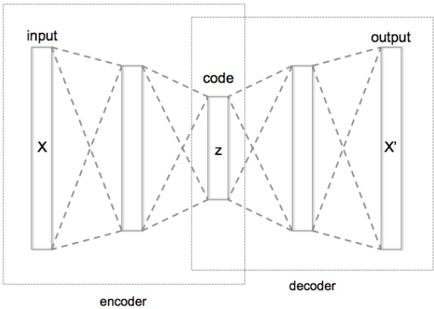
Figure 1: Schematic structure of an Auto encoder with Three fully connected hidden layers. The code $(z)$ is the most internal layer.
图 1: 具有三个全连接隐藏层的自编码器 (Auto encoder) 结构示意图。最内层为编码 $(z)$。
Additionally, we review and summarize some publications which utilize Auto encoder, and they will be discussed in the following sub-sections.
此外,我们回顾并总结了一些利用自动编码器 (Auto encoder) 的文献,这些内容将在以下小节中讨论。
2.2. Auto encoder based Recommendation Models
2.2. 基于自编码器 (Autoencoder) 的推荐模型
Auto encoder is an unsupervised model attempting to reconstruct its input data in the output layer. In general, the bottleneck layer (the middle-most layer) is used as a salient feature representation of the input data (Zhang et al., 2019). The schematic of basic Auto encoder is illustrated in Figure 1, which output $X^{\prime}$ should become closer to the input $X$ and the bottleneck layer is shown by $z$ . The main variants of Auto encoders can be considered as denoising Autoencoder, marginalized denoising Auto encoder, sparse Autoencoder, contractive Auto encoder and variation al Auto encoder (Goodfellow et al., 2016).
自编码器 (Autoencoder) 是一种无监督模型,旨在输出层重构输入数据。通常,瓶颈层(最中间的层)被用作输入数据的显著特征表示 (Zhang et al., 2019)。基础自编码器的结构如图 1 所示,其输出 $X^{\prime}$ 应趋近于输入 $X$,瓶颈层由 $z$ 表示。自编码器的主要变体包括去噪自编码器、边缘化去噪自编码器、稀疏自编码器、收缩自编码器和变分自编码器 (Goodfellow et al., 2016)。
There are two general ways to apply Auto encoder to a recommend er system (Zhang et al., 2019):
将自动编码器 (Auto encoder) 应用于推荐系统 (recommend er system) 主要有两种通用方法 (Zhang et al., 2019):
Almost all the Auto encoder variants such as denoising Auto encoder, variation al Auto encoder, contractive Autoencoder, and marginalized Auto encoder can be applied to the recommendation task. In this paper, we employed the first technique to extract new low-dimension features. Figure 1 illustrates the structure of different recommendation models based on Auto encoder (Zhang et al., 2019).
几乎所有自编码器变体,如去噪自编码器、变分自编码器、收缩自编码器和边缘化自编码器,均可应用于推荐任务。本文采用第一种技术来提取新的低维特征。图1展示了基于自编码器的不同推荐模型结构 (Zhang et al., 2019)。
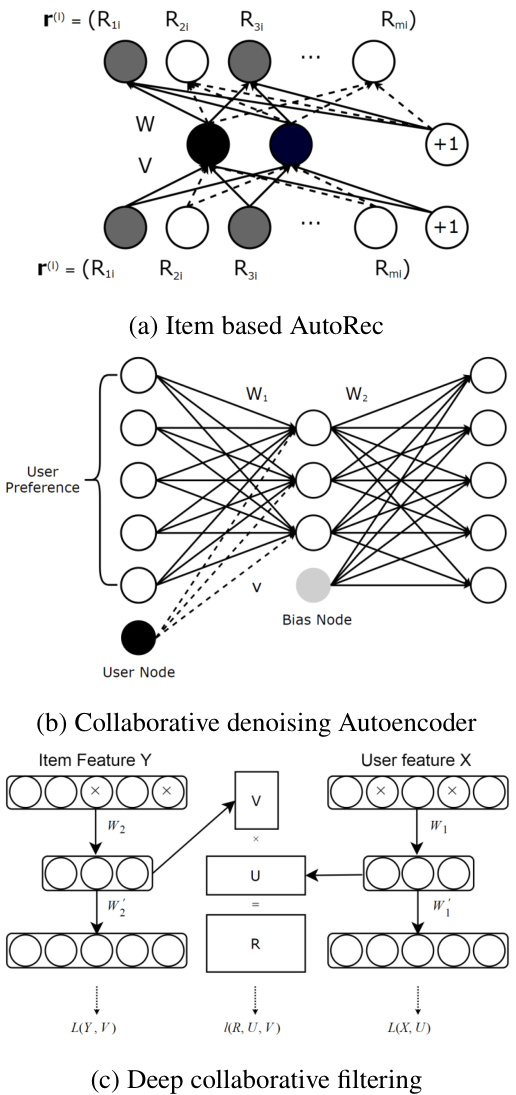
Figure 2: Illustration of: (a) Item based AutoRec; (b) Collaborative denoising Auto encoder; (c) Deep collaborative filtering framework (Zhang et al., 2019)
图 2: 示意图:(a) 基于项目的 AutoRec;(b) 协同去噪自编码器;(c) 深度协同过滤框架 (Zhang et al., 2019)
2.2.1. Auto encoder based Collaborative Filtering Models
2.2.1. 基于自编码器 (Autoencoder) 的协同过滤模型
One of the successful applications is to consider collaborative filtering from the Auto encoder perspective. AutoRec (Sedhain et al., 2015) took user partial vectors $r^{(u)}$ or item partial vectors $r^{(i)}$ as input and attempted to reconstruct them in the output layer. Indeed, it has two variants: item-based AutoRec (I-AutoRec) and user-based AutoRec (U-AutoRec), corresponding to the two types of inputs.
其中一个成功的应用是从自动编码器 (Auto encoder) 角度考虑协同过滤。AutoRec (Sedhain et al., 2015) 将用户部分向量 $r^{(u)}$ 或物品部分向量 $r^{(i)}$ 作为输入,并尝试在输出层重建它们。实际上,它有两种变体:基于物品的 AutoRec (I-AutoRec) 和基于用户的 AutoRec (U-AutoRec),分别对应两种输入类型。
There are essential points about AutoRec that worth noticing (Zhang et al., 2019). First, I-AutoRec performs better than U-AutoRec, which may be due to the higher variance of user partially observed vectors. Second, a different combination of activation functions will influence the performance significantly. Third, moderately increasing the hidden unit size will improve the result as expanding the hidden layer dimensionality gives AutoRec more capacity to model the input characteristics. Furthermore, adding more layers to formulate a deep network can lead to slight improvement.
关于AutoRec有几个关键点值得注意 (Zhang et al., 2019) 。首先,I-AutoRec的表现优于U-AutoRec,这可能是因为用户部分观测向量的方差更大。其次,不同的激活函数组合会显著影响性能。第三,适度增加隐藏单元数量可以改善结果,因为扩大隐藏层维度使AutoRec有更强的能力来建模输入特征。此外,增加更多层以构建深层网络可以带来轻微提升。
CFN (Strub et al., 2016; Strub and Mary, 2015) is a continuation of AutoRec, and posses the following two improve
CFN (Strub et al., 2016; Strub and Mary, 2015) 是 AutoRec 的延续,并具备以下两项改进
ments:
注释:
The CFN input is also partially observed vectors, so it also has two variants: I-CFN and U-CFN, taking $r^{(i)}$ and $r^{(u)}$ as input, respectively. Masking noise is imposed as a great regularize r to better deal with missing elements (with zero value). Further extension of CFN also incorporates side information. However, instead of just integrating side information in the first layer, CFN injects side information in every layer (Zhang et al., 2019).
CFN的输入同样是部分观测向量,因此它也有两个变体:I-CFN和U-CFN,分别以$r^{(i)}$和$r^{(u)}$作为输入。掩码噪声被用作强正则化器,以更好地处理缺失元素(值为零的情况)。CFN的进一步扩展还整合了辅助信息。然而,与仅在首层集成辅助信息不同,CFN在每一层都注入了辅助信息 (Zhang et al., 2019)。
Collaborative Denoising Auto encoder (CDAE). The three models reviewed earlier are mainly designed for rating prediction, while CDAE (Wu et al., 2016) is principally used for ranking prediction. The input of CDAE is user partially observed implicit feedbacks. If the user likes the movie, the entry value is one, otherwise zero. It can also be considered as a preference vector that reflects the user’s interests in items (Zhang et al., 2019). Figure 1b illustrates the structure of CDAE.
协同去噪自编码器 (Collaborative Denoising Autoencoder, CDAE)。之前回顾的三种模型主要针对评分预测设计,而CDAE (Wu等人,2016) 主要用于排序预测。CDAE的输入是用户部分观察到的隐式反馈:若用户喜欢某部电影,则对应项为1,否则为0。该输入也可视为反映用户对物品兴趣的偏好向量 (Zhang等人,2019)。图1b展示了CDAE的结构。
This model uses a unique weight matrix for each user and has a notable impact on model performance. Parameters of CDAE are also learned by minimizing the reconstruction error. CDAE initially updates its parameters using SGD overall feedbacks. However, it is impractical to consider all ratings in real-world applications. A negative sampling technique has been proposed to sample a small subset from the negative set (items with which the user has not interacted), which reduces the time complexity substantially without degrading the ranking quality (Zhang et al., 2019).
该模型为每位用户使用独特的权重矩阵,并对模型性能产生显著影响。CDAE的参数同样通过最小化重构误差来学习。CDAE最初使用SGD(随机梯度下降)基于全部反馈更新参数。然而在实际应用中,考虑所有评分是不现实的。已有研究提出负采样技术,从负样本集(用户未交互过的物品)中抽取小子集,这在不降低排序质量的前提下大幅降低了时间复杂度 (Zhang et al., 2019)。
Muli-VAE and Multi-DAE (Liang et al., 2018) proposed a variant of variation al Auto encoder for recommendation with implicit data, showing better performance than CDAE. These methods introduced a principled Bayesian inference approach for parameter estimation and showed agreeable results than generally used likelihood functions.
多任务变分自编码器 (Multi-VAE) 和多任务去噪自编码器 (Multi-DAE) (Liang et al., 2018) 提出了一种针对隐式数据的推荐系统变分自编码器变体,其性能优于协同去噪自编码器 (CDAE)。这些方法采用贝叶斯推断框架进行参数估计,相比传统似然函数取得了更优的结果。
Based on a survey by Zhang et al. (2019), Auto encoderbased Collaborative Filtering (ACF) (Ouyang et al., 2014) is the first Auto encoder based collaborative recommendation model. Instead of using the original partial observed vectors, it decomposes them by integer ratings. Like AutoRec and CFN, ACF aims at reducing the mean squared error as the cost function. But, there are two demerits of ACF; it loses to deal with non-integer ratings, and the decomposition of partially observed vectors increases the sparseness of input data and drives to worse prediction accuracy.
根据Zhang等人(2019)的调查,基于自编码器的协同过滤(ACF)(Ouyang等人,2014)是首个基于自编码器的协同推荐模型。该模型不使用原始的部分观测向量,而是通过整数评分对其进行分解。与AutoRec和CFN类似,ACF旨在将均方误差作为成本函数进行优化。但ACF存在两个缺点:无法处理非整数评分,且部分观测向量的分解增加了输入数据的稀疏性,导致预测精度下降。
2.2.2. Feature Representation Learning with Auto encoder
2.2.2. 基于自动编码器 (Auto encoder) 的特征表示学习
Auto encoder is a dominant feature representation learning approach, and it can be used in recommend er systems to learn feature representations from users-items content features. In the following, we will summarize some of the related methods.
自动编码器 (Auto encoder) 是一种主流的特征表示学习方法,可用于推荐系统中从用户-物品内容特征中学习特征表示。接下来我们将总结部分相关方法。
Collaborative Deep Learning (CDL) (Wang et al., 2015) is a hierarchical Bayesian model that integrates stacked denoising Auto encoder (SDAE) into probabilistic matrix factorization. The method proposed a general Bayesian deep learning framework (Wang and Yeung, 2016) to combine the deep learning and recommendation model. The framework consists of two tightly coupled parts: the perception component (deep neural network) and task-specific component. Mainly, CDL’s perception component is a probabilistic represent ation of ordinal SDAE, and PMF (Probability Mass Function) works as the task-specific component. This tight combination enables CDL to balance the impacts of side information and interaction records.
协同深度学习 (Collaborative Deep Learning, CDL) [20] 是一种分层贝叶斯模型,它将堆叠去噪自编码器 (SDAE) 整合到概率矩阵分解中。该方法提出了一个通用的贝叶斯深度学习框架 [21],用于结合深度学习与推荐模型。该框架由两个紧密耦合的部分组成:感知组件 (深度神经网络) 和任务特定组件。其中,CDL 的感知组件是序数 SDAE 的概率表示,而概率质量函数 (PMF) 则作为任务特定组件。这种紧密组合使 CDL 能够平衡辅助信息和交互记录的影响。
Collaborative Deep Ranking (CDR). CDR (Ying et al., 2016) is devised specifically in a pairwise framework for topn recommendation. Some studies have demonstrated that the pairwise model is more suitable for ranking lists generation. Experimental results also show that CDR outperforms CDL in terms of ranking prediction (Zhang et al., 2019).
协同深度排序 (CDR) 。CDR (Ying et al., 2016) 是专门为topn推荐设计的成对排序框架。研究表明,成对模型更适合生成排序列表。实验结果也表明,CDR在排序预测方面优于CDL (Zhang et al., 2019)。
Deep Collaborative Filtering Framework is a general fram work for unifying deep learning approaches with a collaborative filtering model (Li et al., 2015). This framework makes it easy to utilize deep feature learning techniques to build hybrid collaborative models (Zhang et al., 2019). There is a marginalized denoising Auto encoder-based collaborative filtering model (mDA-CF) on top of this framework. In comparison to CDL, mDA-CF explores more computationally efficient variants of the Auto encoder. The method saves the computational costs of searching sufficient corrupted input by marginal i zing the corrupted input, and it makes the mDACF more scalable than CDL. Plus, mDA-CF embeds content information of items and users, while CDL only regards item features’ effects.
深度协同过滤框架是一种通用框架,用于统一深度学习方法与协同过滤模型(Li等人,2015)。该框架便于利用深度特征学习技术构建混合协同模型(Zhang等人,2019)。该框架之上还构建了基于边缘化去噪自编码器的协同过滤模型(mDA-CF)。与CDL相比,mDA-CF探索了计算效率更高的自编码器变体。该方法通过边缘化损坏输入来节省搜索足够损坏输入的计算成本,使得mDA-CF比CDL更具可扩展性。此外,mDA-CF嵌入了项目和用户的内容信息,而CDL仅考虑项目特征的影响。
Auto $\mathrm{SVD++}$ (Zhang et al., 2017) uses contractive Autoencoder (Rifai et al., 2011) to learn item feature representations, then integrates them into the classic recommendation model, $\mathrm{SVD++}$ . The model posses the following advantages (Zhang et al., 2019)
Auto $\mathrm{SVD++}$ (Zhang et al., 2017) 采用收缩自编码器 (Rifai et al., 2011) 学习物品特征表示,并将其整合到经典推荐模型 $\mathrm{SVD++}$ 中。该模型具有以下优势 (Zhang et al., 2019)
HRCD (Wei et al., 2017) is a hybrid collaborative model based on Auto encoder and time $\mathrm{SVD++}$ . It is a time-aware model that uses SDAE to learn item representations from raw features and solve the cold item problem (Zhang et al., 2019).
HRCD (Wei等人,2017) 是一种基于自动编码器 (Auto encoder) 和时间敏感 $\mathrm{SVD++}$ 的混合协同模型。该时间感知模型利用堆叠降噪自编码器 (SDAE) 从原始特征中学习物品表征,以解决冷启动物品问题 (Zhang等人,2019)。
3. Graph-based Hybrid Recommendation System
3. 基于图的混合推荐系统
In this section, we focus on our proposed method which can be categorized as a hybrid recommendation system. First we define the basic notations used throughout the paper. Next, we describe the proposed model in an architectural view and algorithmic steps. Then, graph-based features will be declared separately. Finally, we will explain about the clustering method and how we find the optimum number of clusters.
在本节中,我们重点介绍提出的混合推荐系统方法。首先定义全文使用的基本符号,接着从架构视角和算法步骤描述所提模型,随后单独说明基于图的特征,最后阐述聚类方法及最优簇数的确定方式。
We first define the basic notations used throughout this paper. Given the set of n users, $U={u_{1},...,u_{n}}$ , and the set of m item, $I={i_{1},...,i_{m}}$ , all user-item pairs can be denoted by an n-by-m matrix $R=U{\times}I$ , where the entry $r_{u i}$ indicates the assigned value of implicit feedback of user $u$ to item $i$ . If $r_{u i}$ has been observed (or known), it is represented by a specified rating associated in a specific range and interval; otherwise, a global default rating is zero. We used this matrix to find similarity between users’ preferences. After generating the similarity graph which represents users as nodes and the relations as edges, we extract the features from this graph, $F_{g}={f_{1},...,f_{g}}$ , and preserve them in the n-by $\mathbf{\nabla}^{\cdot}\mathbf{g}$ matrix. We collect some users’ features from the dataset, which are called side information, $F_{u}={f_{1},...,f_{u}}$ , some items’ side information $F_{i}={f_{1},...,f_{i}}$ and obtain the combined feature matrix which is $\mathrm{n{-}b y{-}g{+}s}$ . Without loss of generality, we categorized all the features (both graph features and side information) as binary which enlarged final feature vector for each user.
我们首先定义本文使用的基本符号。给定n个用户的集合$U={u_{1},...,u_{n}}$和m个物品的集合$I={i_{1},...,i_{m}}$,所有用户-物品对可以用一个n×m矩阵$R=U{\times}I$表示,其中元素$r_{u i}$表示用户$u$对物品$i$的隐式反馈赋值。若$r_{u i}$已被观测(或已知),则用特定范围和间隔的指定评分表示;否则全局默认评分为零。我们利用该矩阵计算用户偏好间的相似度。生成以用户为节点、关系为边的相似图后,从中提取特征$F_{g}={f_{1},...,f_{g}}$并保存在n×$\mathbf{\nabla}^{\cdot}\mathbf{g}$矩阵中。我们从数据集中收集部分用户特征(称为辅助信息)$F_{u}={f_{1},...,f_{u}}$和物品辅助信息$F_{i}={f_{1},...,f_{i}}$,最终得到组合特征矩阵$\mathrm{n{-}b y{-}g{+}s}$。为不失一般性,我们将所有特征(包括图特征和辅助信息)二值化处理,从而扩展了每个用户的最终特征向量。
3.1. Architecture
3.1. 架构
The overall structure of our aggregated recommend er system (GHRS) is presented in Figure 3. The Graph-based Hybrid Recommend er System comprises the following seven steps:
我们的聚合推荐系统(GHRS)整体结构如图3所示。基于图的混合推荐系统包含以下七个步骤:
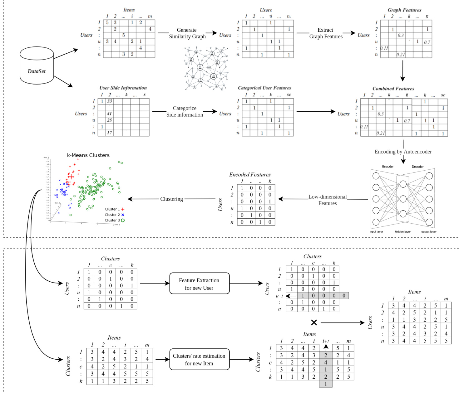
Figure 3: The framework of the proposed recommendation system. The method encodes the combined features with auto encoder and creates the model by clustering the users using the encoded features (upper part). At last, a preference-based ranking model is used to retrieve the predicted movie rank for the target user (lower part)
图 3: 提出的推荐系统框架。该方法通过自动编码器 (auto encoder) 对组合特征进行编码,并利用编码后的特征对用户进行聚类来创建模型 (上半部分)。最后使用基于偏好的排序模型为目标用户检索预测的电影排名 (下半部分)
Algorithm 1 declared the total workflow in details.
算法1详细声明了整体工作流程。
3.2. Graph-based Features
3.2. 基于图 (Graph) 的特征
This section reviews the intuition of some graph features that represent similarities and their general computational process.
本节回顾了一些表示相似性的图特征的直观理解及其通用计算过程。
• Page Rank: Page Rank is an algorithm that measures the transitive influence or connectivity of nodes. It was initially designed as an algorithm to rank web pages (Xing and Ghorbani, 2004). We can compute the Page Rank by either iterative ly distributing one node’s rank (based on the degree) over the neighbors or randomly traversing the graph and counting the frequency of hitting each node during these paths. In this paper, we used the first method.
• Page Rank: Page Rank是一种衡量节点传递影响力或连通性的算法。它最初被设计为网页排序算法 (Xing and Ghorbani, 2004)。我们可以通过迭代地将一个节点的排名(基于度数)分配给邻居节点,或者随机遍历图并统计这些路径中访问每个节点的频率来计算Page Rank。在本文中,我们使用了第一种方法。
• Degree Centrality: Degree centrality measures the number of incoming and outgoing relationships from a node. The Degree Centrality algorithm can be used to find the popularity of individual nodes (Freeman, 1979). The degree centrality values are normalized by dividing by the maximum possible degree in a simple graph n-1, where n is the number of nodes.
• 度中心性 (Degree Centrality): 度中心性衡量节点接收和发出关系的数量。度中心性算法可用于发现单个节点的受欢迎程度 (Freeman, 1979)。度中心性值通过除以简单图中最大可能度数n-1进行归一化,其中n为节点数量。
• Closeness Centrality: Closeness centrality is a way
• 接近中心性 (Closeness Centrality): 接近中心性是一种衡量网络中节点重要性
Input: $U,I,R,F_{u},F_{i}$ Output: Estimated rates for user-item 1: Set alpha $=$ percentage of items with similar ratings between two users 2: Compute the aggregated similarity between users base of $\alpha$ (the percentage of items which two users rated them similarly) 3: Construct the Similarity Graph and consider the users as nodes 4: $F_{g}$ : Extracted graph-based features for users (nodes) 5: $F_{s}$ : Pre processed and categorized users’ side information (demographic informations) 6: Combine $F_{g}$ and $F_{s}$ in a single feature vector $F_{t}$ . Apply the Auto encoder on $F_{t}$ and train the model with the best settings 7: Encode the $F_{t}$ using the Auto encoder an extract the low dimensional feature vector $F_{e}$ 8: Find the optimum clusters for clustering users with $F_{e}$ 9: Perform user clustering using extracted features vector $F_{e}$ and find clusters $C$ 10: Generate the user-cluster matrix $U C$ 11: Estimate clusters’ ratings for items matrix $C I$ : 12: if there are users rated the item i before in the cluster $c$ then 13: $C I_{c i}=$ average (users’ rates of the item $i$ in the cluster $c$ ) 14: else if there are Similar Items to the item $i$ , rated by users in the cluster $c$ then 15: $C I_{c i}=$ average (users’ rates of Similar Items in the cluster $c$ ) 16: else 17: $C I_{c i}=$ average (all users’ rates in the cluster $c$ ) 18: end if 19: Estimate users’ ratings’ matrix $R^{\prime}=U C\times C I$ 20: Compute the recommendation list for target user $u$
输入:$U,I,R,F_{u},F_{i}$
输出:用户-物品的预估评分
1: 设置alpha $=$ 两位用户间评分相似物品的百分比
2: 基于$\alpha$计算用户间的聚合相似度(两位用户评分相似的物品百分比)
3: 构建相似度图,将用户视为节点
4: $F_{g}$:为用户(节点)提取基于图的特征
5: $F_{s}$:预处理并分类的用户辅助信息(人口统计信息)
6: 将$F_{g}$和$F_{s}$合并为单一特征向量$F_{t}$。对$F_{t}$应用自动编码器并以最佳设置训练模型
7: 使用自动编码器编码$F_{t}$并提取低维特征向量$F_{e}$
8: 用$F_{e}$寻找用户聚类的最优簇数
9: 使用提取的特征向量$F_{e}$进行用户聚类,得到簇$C$
10: 生成用户-簇矩阵$UC$
11: 预估簇对物品的评分矩阵$CI$:
12: 若簇$c$中有用户曾对物品$i$评分则
13: $CI_{ci}=$ 簇$c$中用户对物品$i$评分的平均值
14: 否则若簇$c$中有用户对物品$i$的相似物品评分则
15: $CI_{ci}=$ 簇$c$中用户对相似物品评分的平均值
16: 否则
17: $CI_{ci}=$ 簇$c$中所有用户评分的平均值
18: 结束条件
19: 预估用户评分矩阵$R^{\prime}=UC \times CI$
20: 为目标用户$u$生成推荐列表
to detect nodes that can spread information efficiently through a graph (Freeman, 1979). The closeness centrality of a node u measures its average farness (inverse distance) to all $\mathrm{n}{-}1$ other nodes. Since the sum of distances depends on the number of graph nodes, closeness is normalized by the sum of the minimum possible distances $n-1$ .
检测图中能高效传播信息的节点 (Freeman, 1979)。节点u的接近中心性衡量其到所有其他$\mathrm{n}{-}1$个节点的平均远度(距离倒数)。由于距离总和取决于图的节点数,接近度通过最小可能距离$n-1$的总和进行归一化。

where $d(v,u)$ is the shortest-path distance between $v$ and $u$ , and $n$ is the number of nodes in the graph. Nodes with a high closeness score have the shortest distances to all other nodes.
其中 $d(v,u)$ 表示节点 $v$ 和 $u$ 之间的最短路径距离,$n$ 是图中的节点总数。接近度得分高的节点到所有其他节点的距离最短。
• Betweenness Centrality: Betweenness centrality is a factor which we use to detect the amount of influence a node has over the flow of information in a graph. It is often used to find nodes that serve as a bridge from one part of a graph to another (Moore, 1959). The Betweenness Centrality algorithm calculates the shortest (weighted) path between every pair of nodes in a connected graph, using the breadth-first search algorithm (Moore, 1959). Each node receives a score, based on the number of these shortest paths that pass through the node. Nodes that most frequently lie on these shortest paths will have a higher betweenness centrality score.
• 介数中心性 (Betweenness Centrality): 介数中心性是我们用来检测节点在图信息流中影响力大小的指标。该指标常用于发现连接图中不同部分的桥接节点 (Moore, 1959)。介数中心性算法通过广度优先搜索算法 (Moore, 1959) 计算连通图中每对节点之间的最短(加权)路径,根据通过该节点的最短路径数量为每个节点评分。最频繁出现在这些最短路径上的节点将获得更高的介数中心性分数。
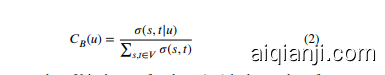
where $V$ is the set of nodes, $\sigma(s,t)$ is the number of shortest path between $(s,t)$ , and $\sigma(s,t|u)$ is the number of those paths passing through some node $u$ other than $s$ and $t$ . If $s=t\to\sigma(s,t)=1$ , and if $v\in{s,t}\rightarrow$ $\sigma(s,t|u)=0$ (Brandes, 2008).
其中 $V$ 是节点集合,$\sigma(s,t)$ 是 $(s,t)$ 之间的最短路径数量,$\sigma(s,t|u)$ 是经过节点 $u$ (除 $s$ 和 $t$ 外) 的最短路径数量。若 $s=t\to\sigma(s,t)=1$,且当 $v\in{s,t}\rightarrow$ $\sigma(s,t|u)=0$ (Brandes, 2008)。
• Load Centrality. The load centrality of a node is the fraction of all shortest paths that pass through that node (Newman, 2001).
• 负载中心性 (Load Centrality)。节点的负载中心性是指所有最短路径中经过该节点的比例 (Newman, 2001)。
• Average Neighbor Degree. Returns the average degree of the neighborhood of each node. The average degree of a node i is:
• 平均邻居度 (Average Neighbor Degree)。返回每个节点邻域的平均度值。节点i的平均度计算公式为:

where $N(u)$ are the neighbors of node $u$ and $k_{v}$ is the degree of node $v$ which belongs to $N(u)$ . For weighted graphs, an analogous measure can be defined (Barrat et al., 2004),
其中 $N(u)$ 是节点 $u$ 的邻居集合,$k_{v}$ 是属于 $N(u)$ 的节点 $v$ 的度数。对于加权图,可以定义类似的度量 (Barrat et al., 2004)。

where $s_{u}$ is the weighted degree of node $u$ , $w_{u v}$ is the weight of the edge that links $u$ and $v$ , and $N(u)$ are the neighbors of node $u$ .
其中 $s_{u}$ 是节点 $u$ 的加权度, $w_{u v}$ 是连接 $u$ 和 $v$ 的边权重, $N(u)$ 是节点 $u$ 的邻居集合。
3.3. User Clustering
3.3. 用户聚类
As we mentioned before in section 3.1, each user belongs to a specific cluster and the cluster rate for an item will be considered as the estimated rating for the user-item pair. In the proposed method we use K-Mean algorithm to cluster the users based on extracted features by Auto encoder. One important issue in using such algorithms is to find the proper number of clusters regarding performance factors. We use two methods to choose the number of clusters; Elbow method and Average Silhouette algorithm.
正如我们在3.1节所述,每个用户都属于特定聚类簇,项目(Item)的簇评分将被视为用户-项目对的预估评分。本方案采用K-Means算法对通过自动编码器(Auto encoder)提取的特征进行用户聚类。使用此类算法的关键问题在于根据性能指标确定最佳聚类数量。我们采用两种方法选择聚类数量:肘部法则(Elbow method)和平均轮廓系数算法(Average Silhouette algorithm)。
In this section we will explain the summary of K-Mean algorithms and how we tackle and solve the number of clusters issue with both mentioned methods.
在本节中,我们将解释K-Means算法的概要,以及如何通过上述两种方法应对并解决聚类数量问题。
3.3.1. K-Means Algorithm
3.3.1. K-Means算法
The K-means algorithm is a simple iterative clustering algorithm. Using the distance as the metric and given the K classes in the data set, calculate the distance mean, giving the initial centroid, with each class described by the centroid (Yuan and Yang, 2019; Awad and Khanna, 2015). For a given data set X with n data samples and the number of category K, the Euclidean distance is the measure of the similarity index, and the clustering method aims minimize the sum of the squares of the various types. It means that it minimizes (Wang et al., 2012)
K-means算法是一种简单的迭代聚类算法。该算法以距离为度量标准,在给定数据集中K个类别的情况下,计算距离均值以确定初始质心,每个类别由质心描述 (Yuan and Yang, 2019; Awad and Khanna, 2015)。对于包含n个数据样本的数据集X和类别数K,欧氏距离(Euclidean distance)作为相似性指标,聚类方法旨在最小化各类别平方和,即最小化 (Wang et al., 2012)

where $k$ represents $K$ cluster centers, $u_{k}$ represents the $k^{t h}$ center, and $x_{i}$ represents the $i^{t h}$ point in the data set.
其中 $k$ 代表 $K$ 个聚类中心,$u_{k}$ 代表第 $k^{t h}$ 个中心,$x_{i}$ 代表数据集中的第 $i^{t h}$ 个点。
3.3.2. Elbow Method
3.3.2. 肘部法则
The basic idea behind cluster partitioning methods, such as k-means clustering, is to define clusters such that the total intra-cluster variation (known as a total within-cluster variation or total within-cluster sum of squares) is minimized. It measures the compactness of the clusters, and it should be as small as possible (Kaufman and Rousseeuw, 2009). The elbow method is based on plotting the explained variation as a function of the number of clusters, and picking the elbow of the output curve as the proper number of clusters. Adding another cluster after the the elbow point doesn’t give much better modeling of the data and may causes over-fitting.
聚类划分方法(如k-means聚类)的基本思想是定义聚类,使得总簇内变异(称为总簇内变异或总簇内平方和)最小化。该方法衡量了簇的紧凑性,其值应尽可能小(Kaufman和Rousseeuw,2009)。肘部法基于绘制解释变异随聚类数量变化的曲线,并选取曲线拐点作为合适的聚类数量。在拐点之后增加更多聚类不会显著提升数据建模效果,反而可能导致过拟合。
3.3.3. Average Silhouette
3.3.3. 平均轮廓系数
Briefly, the average silhouette approach measures the quality of a clustering. It means that it determines how well each object occupies within its cluster. A high average silhouette width intimates a valuable clustering.
简而言之,平均轮廓法用于衡量聚类的质量。它通过评估每个对象在其所属聚类中的匹配程度来实现这一目的。较高的平均轮廓宽度值通常表明聚类效果良好。
The average silhouette method computes the average silhouette of observations for different values of k. The optimal number of clusters $\mathrm{k\Omega}$ is the one that maximizes the average silhouette over a range of possible values for $k$ (Kaufman and Rousseeuw, 2009).
平均轮廓方法计算不同k值下观测值的平均轮廓。最佳聚类数$\mathrm{k\Omega}$是在$k$的可能取值范围内使平均轮廓最大化的那个值 (Kaufman and Rousseeuw, 2009)。
4. Empirical Experiments and Performance Evaluation
4. 实证实验与性能评估
In this section, the performance of the proposed model is evaluated, analyzed, and enumerated in separate parts. The dataset is processed and described in detail, followed by the requisite experimental setup. Due to the variation of steps and processes in the proposed method, we elaborate on the practical results in-depth. Finally, we compared the method with basics and modern methods, which we discussed most of them in related works.
本节从多个独立部分对提出模型的性能进行评估、分析和列举。首先详细处理和描述数据集,随后介绍必要的实验设置。由于所提方法的步骤和流程存在差异,我们将深入阐述实际实验结果。最后,我们将该方法与基础方法及现代方法进行对比(其中大部分方法已在相关工作部分讨论过)。
4.1. Dataset
4.1. 数据集
We have utilized two benchmark datasets (MovieLens 100K and MovieLens 1M) of the real-world in recommend er systems to implement the model practically (Harper and Konstan, 2015). MovieLens 100K contains 100,000 ratings $R\in$ {1, 2, 3, 4, 5}, 1,682 movies (items) rated by 943 users. MovieLens 1M comprises of 1,000,209 ratings $R\in{1,2,3,4,5}$ of approximately 3,900 movies made by 6,040 users. As discussed in Section 3, the proposed method uses users’ demographic data to solve the new users’ cold-start issue. Hence, due to the lack of users’ demographic data in larger datasets like MovieLens 10M, it would not be possible to evaluate the model more on larger datasets. We used the MovieLens 100K dataset for analyzing the proposed method’s steps. The final evaluations and comparisons have been done on the MovieLense 1M dataset. Table 1 shows the details of the mentioned datasets.
我们使用了推荐系统领域两个真实场景的基准数据集(MovieLens 100K和MovieLens 1M)来实际验证模型(Harper和Konstan,2015)。MovieLens 100K包含100,000条评分$R\in${1,2,3,4,5},涉及943位用户对1,682部电影(项目)的评分。MovieLens 1M包含6,040位用户对约3,900部电影给出的1,000,209条评分$R\in{1,2,3,4,5}$。如第3节所述,本方法利用用户人口统计数据解决新用户冷启动问题。因此,由于MovieLens 10M等更大规模数据集缺乏用户人口统计数据,无法在更大数据集上进一步评估模型。我们使用MovieLens 100K数据集分析所提方法的各个步骤,最终评估与对比则在MovieLens 1M数据集上完成。表1展示了上述数据集的详细信息。
4.2. Features Statistics
4.2. 特征统计
As declared in Section 3, we use two types of features in the proposed method: side information (users’ demographic data) and features extracted from the similarity graph between users. We transformed the demographic data into a categorical format, concatenated both types of features, and made the raw feature set before dimension reduction with an Auto encoder. In this section, we discuss a little about the statistics of the raw features.
如第3节所述,我们在所提方法中使用两类特征:辅助信息(用户人口统计数据)和从用户相似度图中提取的特征。我们将人口统计数据转换为分类格式,拼接两类特征,并通过自动编码器(Auto encoder)进行降维前形成原始特征集。本节简要讨论原始特征的统计信息。
We have declared before the only parameter we have used for generating the graph is $\alpha$ , the value of a threshold for connecting two users having at least several same movies in their ratings. This threshold is represented as a percentage of total movies in the dataset. Hence, we have an exploration of a very sparse graph to near a full-mesh graph. Figure 4 illustrates the similarity graph visualization for $\alpha=$ $\left{0.005,0.01,0.02,0.03\right}$ for 943 users in MovieLens 100K.
我们之前声明过,生成该图所使用的唯一参数是 $\alpha$,即连接两位评分中至少有部分相同电影的用户时的阈值。该阈值以数据集中电影总数的百分比表示。因此,我们从极稀疏图探索至接近全连接图的状态。图 4 展示了 MovieLens 100K 数据集中 943 位用户在 $\alpha=$ $\left{0.005,0.01,0.02,0.03\right}$ 时的相似度图可视化结果。
Figure 5 shows the normalized graph-based features’ distributions against each other for MovieLens 100K and MovieLens 1M with $\alpha=0.015$ . We can see correlations between these types of features in some cases.
图 5: 展示了 MovieLens 100K 和 MovieLens 1M 在 $\alpha=0.015$ 时基于图的归一化特征之间的分布情况。可以看出在某些情况下这些特征类型之间存在相关性。
As all the demographic features are transformed into a categorical format, the demographic features vector is onehot encoded and has a specific sparsity level for each dataset. On the other hand, we declared that the graph-based features’ value is related to the similarity graph size, and the graph size is directly related to the factor $\alpha$ . In Figure 6, we can see that the feature set’s sparsity rises when the value of the $\alpha$ increases.
由于所有人口统计特征均转换为分类格式,人口统计特征向量经过独热编码后,各数据集具有特定的稀疏度。另一方面,我们声明基于图的特征值与相似图规模相关,而图规模直接受参数$\alpha$影响。图6显示,当$\alpha$值增大时,特征集的稀疏度随之上升。
4.3. Performance Metrics
4.3. 性能指标
We use 10-fold cross-validation on MovieLens 1M datase and 5-fold cross-validation on MovieLens 100K dataset to partition the datasets into training and testing to measure the performance of the GHRS. The final prediction metrics are the average of the iterations of training and testing base on the number of folds in each dataset. The training set comprises the User-Item list with given ratings, user’s demographic information, and item’s side information. We consider the Root Mean Squared Error (RMSE) as the metric for evaluation. RMSE (Equation 6) is generally related to the cost function of conventional rating prediction models:
我们在MovieLens 1M数据集上采用10折交叉验证,在MovieLens 100K数据集上采用5折交叉验证,将数据集划分为训练集和测试集以评估GHRS的性能。最终预测指标是基于每个数据集的折数对训练和测试迭代结果取平均值。训练集包含带有给定评分的用户-项目列表、用户人口统计信息以及项目辅助信息。我们选用均方根误差(RMSE)作为评估指标。RMSE(公式6)通常与传统评分预测模型的损失函数相关:
Table 1 Details of the datasets used for evaluation
表 1: 用于评估的数据集详细信息

Figure 4: Visualization of Similarity Graph for $\alpha={0.005,0.01,0.02,0.03}$ for MovieLens 100K with 943 users.
图 4: MovieLens 100K数据集(包含943位用户)在$\alpha={0.005,0.01,0.02,0.03}$参数下的相似度图可视化。

Where $U$ is user set, $I$ is item set, and $R_{u i}$ and $R_{u i}^{\prime}$ are the actual and predicted ratings of user $u$ for item $i$ , respectively.
其中 $U$ 为用户集合, $I$ 为物品集合, $R_{u i}$ 和 $R_{u i}^{\prime}$ 分别表示用户 $u$ 对物品 $i$ 的实际评分与预测评分。
Besides those mentioned above, we also use Precision and Recall (the most popular metrics for evaluating information retrieval systems) as an evaluation metric to measure the proposed model’s accuracy. Precision measures the ratio of correct recommendations to the total recommendations, and Recall shows the ratio of correct recommendations to total correct information. Consequently, we have to separate the items into two classes with a threshold while considering their actual ratings, i.e., non-relevant and relevant to measure Precision and Recall. In this regard, items rated between $[1-3]$ were considered non-relevant and rated with [4 − 5] as relevant. Additionally, the items in datasets were divided as selected and not selected on their predicted ratings. Therefore, Precision and Recall of the model can be defined as:
除上述指标外,我们还采用精确率 (Precision) 和召回率 (Recall) 这两个信息检索系统最常用的评估指标来衡量所提模型的准确性。精确率衡量正确推荐占总推荐的比例,召回率则反映正确推荐占全部正确信息的比例。为此,我们需要根据实际评分设定阈值将项目分为两类(不相关与相关)来计算精确率和召回率:评分在 $[1-3]$ 区间的项目视为不相关,评分在 [4−5] 区间的项目视为相关。同时,根据预测评分将数据集中的项目划分为被选中和未被选中两类。因此,模型的精确率和召回率可定义为:

召回率 = $$
\frac{TP}{TP + FN}
$$
Where $T P$ stands for True Positive (Item is correctly selected as it is relevant), $F P$ stands for False Positive (Item is incorrectly selected as it is not relevant), and $F N$ stands for False Negative (Relevant item is not selected)
其中 $TP$ 表示真正例 (True Positive,相关项被正确选中),$FP$ 表示假正例 (False Positive,不相关项被错误选中),$FN$ 表示假反例 (False Negative,相关项未被选中)
Root Mean Square Error (RMSE) for the proposed model gives a lower error value for the testing dataset. Observed results produced by iterations of cross-validation (10-fold for MovieLens 1M and 5-fold for MovieLens 100K) show almost similar validation errors.
所提模型的均方根误差 (RMSE) 在测试数据集上表现出更低的误差值。通过交叉验证迭代 (MovieLens 1M 采用 10 折,MovieLens 100K 采用 5 折) 观察到的结果显示验证误差几乎相同。
4.4. Impact of similarity graph size
4.4. 相似图大小的影响
In this experiment, we check the impact of graph size on rating accuracy. As we use graph features for every node (users) in the similarity graph, it’s important to produce a similarity graph in a state that represents the similarity between nodes as optimized as it can be. For this purpose, we experimented with searching in parameter space, which impacts the size and the shape of the similarity graph. Figure 7 shows the RMSE vs. $\alpha$ in both dataset we used for the evaluation. As it can be seen in the figure, there is no direct relation between the result of the method. But, the minimum value of RMSE achieved on a specific value of alpha in the middle of the experiment range.
在本实验中,我们检验了图规模对评分准确率的影响。由于我们为相似图中的每个节点(用户)使用图特征,因此生成一个能最优表示节点间相似性的相似图状态至关重要。为此,我们尝试在参数空间中进行搜索,该参数会影响相似图的大小和形状。图7展示了我们用于评估的两个数据集中RMSE与$\alpha$的关系。如图所示,该方法的结果与参数值之间没有直接关联。但RMSE的最小值出现在实验范围中段的某个特定alpha值处。
The main reason for this result is that when the alpha’s value is very small, all users can be connected due to this value because we consider just a very little common items in their ratings to connect them to each other in the similarity graph. Hence, most of the users are similar to each other in this condition and the difference will be missed in some cases. On the other hand, when the alpha’s value raises the similarity graph become more sparse (As it is shown in Figure 6). So, we consider the most of users not related to each other when the $\alpha$ value increases to very large values. There is an optimum point for the size of the similarity graph near the alpha $=0.01$ for dataset MovieLens 100K and near the alpha $=0.005$ for MovieLens 1M. The result of this parameter tuning has been produced with the exact condition of the final evaluation with $\mathrm{k}$ -fold cross-validation (Figure 6).
这一结果的主要原因是,当alpha值非常小时,由于该值考虑了评分中极少的共同项来在相似图中连接用户,因此所有用户都能被连接。在这种情况下,大多数用户彼此相似,某些情况下差异会被忽略。另一方面,当alpha值增大时,相似图会变得更稀疏(如图6所示)。因此,当$\alpha$值增加到非常大时,我们认为大多数用户彼此不相关。对于MovieLens 100K数据集,相似图大小的最佳点出现在alpha$=0.01$附近;而对于MovieLens 1M数据集,最佳点则在alpha$=0.005$附近。该参数调优结果是在与最终评估完全相同的条件下通过$\mathrm{k}$折交叉验证得出的(图6)。
4.5. Dimension Reduction
4.5. 降维
We declared that we use Auto encoder to simultaneously extract new features and reduce the raw feature set dimension before clustering. In this experiment, we examine the learning algorithms for Auto encoder and check each algorithm’s ability to minimize the loss function on our input raw feature set. In all experiments, we have used a 5-layer Auto encoder with the structure shown in Figure 8. The activation function of all layers is ReLU (Nair and Hinton, 2010).
我们声明在聚类前使用自动编码器 (Auto encoder) 同时提取新特征并降低原始特征集维度。本实验测试了自动编码器的学习算法,并检验各算法在输入原始特征集上最小化损失函数的能力。所有实验均采用如图 8 所示的 5 层自动编码器结构,各层激活函数为 ReLU (Nair and Hinton, 2010)。
Both input and output size (raw feature vector’s sizes)
输入和输出大小(原始特征向量的尺寸)

are 35 for MovieLens 100K and 36 for MovieLens 1M.
MovieLens 100K为35,MovieLens 1M为36。
We experiment with a set of optimizers to train the Autoencoder. Optimizers include Adagrad (Duchi et al., 2011), Adadelta (Zeiler, 2012), RMSProp (Hinton et al., 2012), Adam (Kingma and Ba, 2017), AdaMax (Kingma and Ba, 2017), Nadam (Dozat, 2016) and SGD (Bottou and Bousquet, 2008) with loss function of Mean Squared Error.
我们尝试使用一组优化器来训练自编码器 (Autoencoder)。优化器包括 Adagrad (Duchi et al., 2011)、Adadelta (Zeiler, 2012)、RMSProp (Hinton et al., 2012)、Adam (Kingma and Ba, 2017)、AdaMax (Kingma and Ba, 2017)、Nadam (Dozat, 2016) 以及采用均方误差 (Mean Squared Error) 作为损失函数的 SGD (Bottou and Bousquet, 2008)。
Figure 9 shows the result of the experiment and compares the optimizers in minimizing the loss function on validation data over 100 epochs of training. We have randomly selected $10%$ of users in MovieLens 1M and $20%$ of users in MovieLens 100K as validation data and exclude them from the training set. We can see the best results for Adam, Adadelta, and RMSProp optimizers. As a discussion about the result, RMSprop can be considered as an extension of Adagrad that deals with its radically diminishing learning rates. It is identical to Adadelta, except that Adadelta uses the RMS of pa- rameter updates in the nominator update rule. Adam, finally, adds bias-correction and momentum to RMSprop (Ruder, 2017).
图 9: 展示了实验的结果,并比较了优化器在100轮训练中验证数据上最小化损失函数的表现。我们随机选取了MovieLens 1M中10%的用户和MovieLens 100K中20%的用户作为验证数据,并将它们从训练集中排除。可以看到Adam、Adadelta和RMSProp优化器取得了最佳效果。关于结果的讨论,RMSprop可视为Adagrad的扩展,解决了其学习率急剧下降的问题。它与Adadelta几乎相同,只是Adadelta在分子更新规则中使用了参数更新的均方根(RMS)。而Adam则在RMSprop基础上增加了偏置校正和动量机制 (Ruder, 2017)。

Figure 6: Sparsity of combined features’ dataset vs. $\alpha$ before dimension reduction
图 6: 降维前组合特征数据集的稀疏度与$\alpha$的关系

Figure 5: Graph-based features for (a) MovieLens 100K and (b) MovieLens 1M both for $\alpha=0.015$ . Abbreviation used in the figure: PR (page rank), CD (degree centrality), CC (closeness centrality), CB (betweenness centrality), AND (average neighbor degree), and LC (load centrality). Centrality measures like CD and PR have more correlation than others, and it may be caused by the correlation of ei gen vector centrality and degree centrality in our user graph. It means that users with a high degree of connection are likely connected in many cases. Figure 7: RMSE vs. $\alpha$ . There is an optimum point for $\alpha$ near the alpha $=0.01$ for dataset MovieLens 100K and near the alpha $=0.005$ for MovieLens 1M.
图 5: (a) MovieLens 100K 和 (b) MovieLens 1M 的基于图的特征 ( $\alpha=0.015$ )。图中缩写: PR (Page Rank)、CD (度中心性)、CC (接近中心性)、CB (介数中心性)、AND (平均邻居度)、LC (负载中心性)。CD 和 PR 等中心性度量指标比其他指标更具相关性,这可能是由于用户图中特征向量中心性与度中心性的相关性所致。这意味着高度连接的用户在许多情况下很可能相互关联。
图 7: RMSE 随 $\alpha$ 的变化曲线。对于 MovieLens 100K 数据集,$\alpha$ 的最优点在 0.01 附近;对于 MovieLens 1M 数据集,最优值在 0.005 附近。
RMSprop, Adadelta, and Adam are very similar algorithms that do well in similar conditions. Kingma and Ba (2017) showed that the bias-correction helps Adam slightly exceed RMSprop towards the end of optimization when the gradients become sparser. Hence, Adam seems to be the best option for the optimizer. Recently, many researchers use vanilla SGD without momentum and a simple learning rate annealing schedule (Ruder, 2017). Nevertheless, In our experiment, SGD approaches to achieves a minimum, but it may take longer than other methods.
RMSprop、Adadelta 和 Adam 是非常相似的算法,在类似条件下表现良好。Kingma 和 Ba (2017) 的研究表明,当梯度变得稀疏时,偏差校正有助于 Adam 在优化后期略微超越 RMSprop。因此,Adam 似乎是优化器的最佳选择。最近,许多研究者使用不带动量的普通 SGD (随机梯度下降) 和简单的学习率退火策略 (Ruder, 2017)。尽管如此,在我们的实验中,SGD 能够接近达到最小值,但可能比其他方法耗时更长。

Figure 8: Structure of Auto encoder used for dimension reduction. Both input and output size are 35 for MovieLens $100\mathsf{K}$ and 36 for MovieLens 1M
图 8: 用于降维的自编码器结构。MovieLens $100\mathsf{K}$ 的输入和输出大小均为35,MovieLens 1M 的输入和输出大小均为36

Figure 9: The value of loss function on validation data over 100 epochs of training with seven target optimizers in the experiment
图 9: 实验中七种目标优化器在100轮训练过程中验证数据上的损失函数值
We selected Adam as the optimizer in Auto encoder to encode the raw feature set. The output of the encoding process shows a diverse distribution with a low correlation between the encoded features. Figure 11 shows the encoded features for both MovieLens 100K and MovieLens 1M, which will be used for clustering the users.
我们在自动编码器中选择Adam作为优化器来编码原始特征集。编码过程的输出显示出多样化的分布,且编码特征间相关性较低。图11展示了MovieLens 100K和MovieLens 1M的编码特征,这些特征将用于用户聚类。
We use elastic net regular iz ation (linear combination of $L_{1}$ and $L_{2}$ penalties) (Zou and Hastie, 2005) for Autoencoder to avoid the over fitting on the training data and improve the model’s performance.
我们采用弹性网络正则化 (elastic net regularization) (线性组合 $L_{1}$ 和 $L_{2}$ 惩罚项) (Zou and Hastie, 2005) 来训练自编码器 (Autoencoder),以避免模型在训练数据上过拟合并提升其性能。
4.6. Number of Clusters
4.6. 聚类数量
This section examines the mentioned method in section 3.3 to find the correct number of clusters for both datasets MovieLens 1M and MovieLens 100K. As listed before, we applied two methods for this reason; the Elbow method and the Average Silhouette method. The input of both methods is the encoded feature sets from the previous state. For both methods, we consider the range of K in $[1-30]$ . Figure 11 and Figure 12 show the algorithms’ iteration for the Elbow method and Average Silhouette method, respectively. The best value of K has been founded, as shown in Table 2.
本节对3.3节中提到的MovieLens 1M和MovieLens 100K两个数据集进行聚类数量确定方法的检验。如前所述,我们采用了两种方法:肘部法则(Elbow method)和平均轮廓系数法(Average Silhouette method)。两种方法的输入均为前一阶段生成的编码特征集,K值搜索范围设定为$[1-30]$。图11和图12分别展示了肘部法则和平均轮廓系数法的算法迭代过程,最终确定的K值最优解如表2所示。

Figure 10: Final Features Scatter (Dimension is reduced to 4 using Auto encoder with Adam optimizer).
图 10: 最终特征散点图 (使用带Adam优化器的自动编码器将维度降至4)。

Figure 11: Finding the elbow point as the optimum number of clusters of users. (a) K-Mean Algorithm. (b) MiniBatchKMean Algorithm
图 11: 寻找肘部点作为用户聚类的最优数量。(a) K均值算法。(b) 小批量K均值算法
4.7. Results and Comparison with Other Methods
4.7. 结果与其他方法的对比
Performance of the proposed model has been evaluated on the datasets mentioned in section 4.1. Table 3 shows the result of the proposed model based on the best setting derived from the experiments conducted to find the best values for parameters $\alpha$ (section 4.4) and K (section 4.6), and best optimizer for Auto encoder (section 4.5).
所提模型的性能已在4.1节所述数据集上进行评估。表3展示了基于最佳参数配置的实验结果,这些参数包括通过实验确定的$\alpha$(4.4节)和K(4.6节)最优值,以及自编码器(Auto encoder)的最佳优化器选择(4.5节)。
In another experiment, we are going to assess the GHRS method in tackling the cold-start problem. For this reason, we had to produce a synthetic dataset from the original dataset like MovieLens $100\mathrm{k\Omega}$ or 1M. In the synthetic dataset, regardless of the number of ratings, we have randomly removed a specific percentage of records from matrix $R$ (user-item ratings) before generating graph-based features for each user. Hence, it has the same condition as a new user without any previous rating records, and we have only side information to predict ratings for this user. Figure 13 shows the method performance result versus the percentage of users which have been randomly removed from the user-item rating matrix. We can see that GHRS delivers a good performance in coldstart issues, even in a high percentage of new users.
在另一项实验中,我们将评估GHRS方法解决冷启动问题的能力。为此,我们基于MovieLens $100\mathrm{k\Omega}$ 或1M等原始数据集生成了合成数据集。在合成数据集中,无论评分数量多少,我们在为每个用户生成基于图的特征前,都从矩阵 $R$ (用户-物品评分矩阵)随机移除了特定比例的记录。因此,其条件等同于没有任何历史评分记录的新用户,我们仅能依靠辅助信息来预测该用户的评分。图13展示了方法性能结果与被随机移除的用户比例之间的关系。可以看出,即使在高比例新用户情况下,GHRS在冷启动问题上仍表现良好。
Table 2 Value of K suggested by Elbow method and Average Silhouette method
表 2: Elbow 方法和平均轮廓系数法建议的 K 值
| Dataset | Elbowmethod | AverageSilhouettemethod |
|---|---|---|
| MovieLens100K | K=8, DistortionScore=37.11 | K=7, Average Silhouette=18.93 |
| MovieLens1M | K=9, DistortionScore=264.61 | K=7, Average Silhouette=17.53 |

Figure 12: Finding the elbow point as the optimum number of clusters of users. (a) K-Mean Algorithm. (b) MiniBatchKMean Algorithm
图 12: 寻找肘部点作为用户聚类的最优数量。(a) K均值算法。(b) 小批量K均值算法
Table 3 Performance metrics value for the proposed method on target dataset
表 3 目标数据集上提出方法的性能指标值
| 数据集 | RMSE | Precision | Recall |
|---|---|---|---|
| 100K | 0.887, S²=1.595×10⁻⁴ | 0.771 | 0.799 |
| 1M | 0.833, S²=2.815×10⁻⁴ | 0.792 | 0.838 |
The proposed method (GHRS) has additionally been compared with some primary methods and state of the art methods. It is evident that the proposed method shows an improvement in the best result of RMSE on MovieLens 1M and has the best performance as same as AutoRec after the Auto encoder COFILS. Full comparison is shown in Table 4.
所提出的方法 (GHRS) 还与一些基础方法和前沿方法进行了比较。显然,该方法在MovieLens 1M数据集上取得了RMSE指标的最佳结果提升,并在自动编码器COFILS之后与AutoRec保持同等最优性能。完整对比结果如 表4 所示。

Figure 13: GHRS method RMSE result versus the percentage of users which have been randomly removed from the user-item rating matrix.
图 13: GHRS方法RMSE结果与被随机移出用户-项目评分矩阵的用户百分比对比
5. Conclusion and Future Works
5. 结论与未来工作
We have proposed a method for the recommendation in user-item systems in this paper. The method can be used for every user-item system that provides side information for both users and items. The proposed method’s main idea is finding the relation between users based on their similarities as nodes in a similarity graph and combining them with the users’ side information to solve the cold-start issue. Plus, we applied Auto encoder to extract new low dimensional features with low correlation and more information. This made the final clustering step more accurate and highly performed in time consumption. Final experiments and comparison with other methods showed the competitive results for the selected datasets and improved the best result on MovieLens 1M dataset.
本文提出了一种用户-物品系统中的推荐方法。该方法适用于所有为用户和物品提供辅助信息的系统。所提方法的核心思想是基于用户作为相似度图中节点的相似性来发现用户间关系,并结合用户辅助信息解决冷启动问题。此外,我们应用自动编码器 (Auto encoder) 提取低相关度且信息量更大的低维新特征,这使得最终聚类步骤更准确且耗时更少。在选定数据集上的最终实验及与其他方法的对比表明,该方法取得了具有竞争力的结果,并在MovieLens 1M数据集上提升了最佳表现。
There are several lines of research arising from this work that should be pursued. Future research might apply for the work on the item properties like user side information to detect similarity between items precisely. Admittedly, it will be like considering similarities between two users who similarly rate the same items, and their rates and properties in the similarity graph are close to each other. Indeed, in this case, items will be considered similar if identical or similar users (based on similarity definition between users in this research) rate them with the same patterns. Thus, we will also have the approach using graph features and deep-learning for users, for items.
从这项工作中可以延伸出多个研究方向。未来的研究可能会应用于物品属性方面的工作,例如利用用户侧信息来精确检测物品间的相似性。诚然,这将类似于考虑对相同物品给出相似评分的两个用户之间的相似性,这些用户在相似性图中的评分和属性彼此接近。实际上,在这种情况下,如果相同或相似的用户(基于本研究中用户间相似性定义)以相同模式对物品进行评分,这些物品将被视为相似。因此,我们还将采用基于图特征和深度学习的方法来处理用户和物品。
On the other hand, it is great to devote future research to developing and extracting more other features from the similarity graph, which we did not mention in the current study. Besides, the structure of the Auto encoder might be an important area for future research. The different structures should be examined regarding the Auto encoder structure affecting feature extraction, training duration, and the model’s final performance. In this article, we used a predefined structure for Auto encoder using the heuristic method and manual tuning. Also, there are many methods to cluster the users in this method. They should be investigated and measured to find the optimal one for this type of feature space and distribution. This assumptions might be addressed in future studies.
另一方面,未来研究可以致力于从相似性图中开发和提取更多其他特征,这些特征在当前研究中未被提及。此外,自编码器 (Auto encoder) 的结构可能是未来研究的重要方向。应针对自编码器结构对特征提取、训练时长及模型最终性能的影响,检验不同结构的差异。本文采用启发式方法和手动调参来预定义自编码器结构。此外,该方法中用户聚类存在多种实现方式,需通过实验评估以确定最适合此类特征空间和分布的最优方案。这些假设或将在后续研究中得到验证。
Table 4 Comparison with other methods
表 4: 与其他方法的对比
| 模型 | MovieLens 100K | MovieLens 1M |
|---|---|---|
| 协同主题回归 (Wang and Blei, 2011) | 0.896 | |
| 协同深度学习 (Wang et al., 2015) | 0.887 | |
| 卷积矩阵分解 (Kim et al., 2016) | 0.853 | |
| 卷积矩阵分解+ (Kim et al., 2016) | 0.854 | |
| 鲁棒卷积矩阵分解 (Kim et al., 2017) | 0.847 | |
| RippleNet (Wang et al., 2018) | 0.863 | |
| 插补奇异值分解 (Yuan et al., 2019) | 0.85 | |
| 遗传算法与引力模拟 (Mohammadpour et al., 2019) | 1.087 | |
| 基于噪声校正的推荐系统 (Bag et al., 2019) | 1.7 | |
| DST-HRS (Khan et al., 2020) | 0.846 | |
| 自编码器 COFILS (Barbieri et al., 2017) | 0.885 | 0.838 |
| 基线 COFILS (Barbieri et al., 2017) | 0.892 | 0.848 |
| 核主成分分析 COFILS (Barbieri et al., 2017) | 0.898 | |
| Slope One (Lemire and Maclachlan, 2005) | 0.937 | 0.9 |
| 正则化奇异值分解 (Paterek, 2007) | 0.989 | 0.96 |
| 改进正则化奇异值分解 (Paterek, 2007) | 0.954 | 0.907 |
| SVD++ (Koren, 2008) | 0.903 | 0.856 |
| 非负矩阵分解 (Lee and Seung, 2001) | 0.944 | 0.912 |
| 贝叶斯概率矩阵分解 (Salakhutdinov and Mnih, 2008) | 0.901 | 0.84 |
| RBM-CF (Salakhutdinov et al., 2007) | 0.936 | 0.872 |
| AutoRec (Sedhain et al., 2015) | 0.887 | 0.844 |
| 均值场 (Langseth and Nielsen, 2015) | 0.903 | 0.856 |
| GHRS (本文方法) | 0.887 | 0.833 |
As discussed in section 4.1, few datasets have side information for users and items(e.g., demographic data for users). It will be desirable to assess the proposed method with other future datasets that include this information.
如第4.1节所述,当前少有数据集包含用户和物品的辅助信息(例如用户人口统计数据)。未来若能获取包含此类信息的数据集,将有助于进一步评估所提出的方法。