Parameter-Efficient Fine-Tuning in Spectral Domain for Point Cloud Learning
点云学习中基于频谱域的参数高效微调
Dingkang Liang, Tianrui Feng, Xin Zhou, Yumeng Zhang, Zhikang Zou, Xiang Bai
Dingkang Liang, Tianrui Feng, Xin Zhou, Yumeng Zhang, Zhikang Zou, Xiang Bai
Abstract—Recently, leveraging pre-training techniques to enhance point cloud models has become a hot research topic. However, existing approaches typically require full fine-tuning of pre-trained models to achieve satisfied performance on downstream tasks, accompanying storage-intensive and computationally demanding. To address this issue, we propose a novel Parameter-Efficient Fine-Tuning (PEFT) method for point cloud, called PointGST (Point cloud Graph Spectral Tuning). PointGST freezes the pre-trained model and introduces a lightweight, trainable Point Cloud Spectral Adapter (PCSA) to fine-tune parameters in the spectral domain. The core idea is built on two observations: 1) The inner tokens from frozen models might present confusion in the spatial domain; 2) Task-specific intrinsic information is important for transferring the general knowledge to the downstream task. Specifically, PointGST transfers the point tokens from the spatial domain to the spectral domain, effectively de-correlating confusion among tokens via using orthogonal components for separating. Moreover, the generated spectral basis involves intrinsic information about the downstream point clouds, enabling more targeted tuning. As a result, PointGST facilitates the efficient transfer of general knowledge to downstream tasks while significantly reducing training costs. Extensive experiments on challenging point cloud datasets across various tasks demonstrate that PointGST not only outperforms its fully fine-tuning counterpart but also significantly reduces trainable parameters, making it a promising solution for efficient point cloud learning. More importantly, it improves upon a solid baseline by $+2.28%$ , $1.16%$ , and $2.78%$ , resulting in $99.48%$ , $97.76%$ , and $96.18%$ on the ScanObjNN OBJ BG, OBJ OBLY, and PB T50 RS datasets, respectively. This advancement establishes a new state-of-the-art, using only $0.67%$ of the trainable parameters. The code will be made available at https://github.com/jerry feng 2003/PointGST.
摘要—最近,利用预训练技术增强点云模型已成为热门研究课题。然而,现有方法通常需要对预训练模型进行全量微调,才能在下游任务上取得满意的性能,这伴随着存储密集和计算需求高的问题。为了解决这一问题,我们提出了一种新颖的点云参数高效微调 (PEFT) 方法,称为 PointGST (点云图谱调优)。PointGST 冻结预训练模型,并引入一个轻量级、可训练的点云谱适配器 (PCSA) 来在谱域微调参数。其核心思想基于两个观察:1) 冻结模型的内部 Token 在空间域中可能会出现混淆;2) 任务特定的内在信息对于将通用知识转移到下游任务非常重要。具体来说,PointGST 将点 Token 从空间域转移到谱域,通过使用正交分量进行分离,有效地解除了 Token 之间的相关性。此外,生成的谱基包含下游点云的内在信息,从而实现更有针对性的调优。因此,PointGST 促进了通用知识向下游任务的高效转移,同时显著降低了训练成本。在各种任务的挑战性点云数据集上进行的大量实验表明,PointGST 不仅优于其全量微调的对应方法,还显著减少了可训练参数,使其成为高效点云学习的一个有前途的解决方案。更重要的是,它在坚实的基础上分别提升了 $+2.28%$、$1.16%$ 和 $2.78%$,在 ScanObjNN OBJ BG、OBJ OBLY 和 PB T50 RS 数据集上分别达到了 $99.48%$、$97.76%$ 和 $96.18%$。这一进展仅使用 $0.67%$ 的可训练参数就建立了新的最先进水平。代码将在 https://github.com/jerry feng 2003/PointGST 上提供。
Index Terms—Point Cloud, Efficient Tuning, Spectral.
索引术语—点云、高效调优、频谱。
1 INTRODUCTION
1 引言
OINT cloud learning is a fundamental and highly practical task within the computer vision community, drawing significant attention due to its extensive applications such as autonomous driving [13], [31], 3D reconstruction [45], [80], and embodied intelligence [82], among others. Different from images, point clouds are inherently sparse, unordered, and irregular, posing unique challenges to effective analysis.
点云学习是计算机视觉领域中一项基础且高度实用的任务,因其广泛的应用(如自动驾驶 [13]、[31]、3D重建 [45]、[80] 以及具身智能 [82] 等)而备受关注。与图像不同,点云本质上是稀疏、无序且不规则的,这为有效分析带来了独特的挑战。
Nowadays, exploring pre-training techniques to boost the models has become a hot research topic in both natural language processing [9] and computer vision [21], and has been successfully transferred to the point cloud domain [36], [47], [75], [85]. For example, representative works like PointBERT [85] and Point-MAE [47] introduce the Mask Point Modeling task for point cloud, and the subsequent studies [4], [11], [36], [93] propose effective customized pretraining tasks. After pre-training, these methods adopt the classical fully fine-training (FFT) strategy, where all models’ parameters are fine-tuned, leading to notable performance improvements and faster convergence compared to training from scratch. However, the FFT incurs significant computational costs, particularly in terms of GPU memory and storage, since fine-tuning the entire pre-trained models involves updating a large number of parameters. With the scaling of models1 or increasing needs to fine-tuning enormous new datasets, the demand for storing fine-tuned checkpoints grows, resulting in heightened storage and memory consumption.
如今,探索预训练技术以提升模型性能已成为自然语言处理 [9] 和计算机视觉 [21] 领域的热门研究课题,并已成功迁移到点云领域 [36], [47], [75], [85]。例如,代表性的工作如 PointBERT [85] 和 Point-MAE [47] 为点云引入了掩码点建模任务,后续的研究 [4], [11], [36], [93] 提出了有效的定制预训练任务。预训练后,这些方法采用了经典的完全微调 (FFT) 策略,即微调所有模型参数,与从头训练相比,显著提升了性能并加快了收敛速度。然而,FFT 会带来巨大的计算成本,尤其是在 GPU 内存和存储方面,因为微调整个预训练模型涉及更新大量参数。随着模型的扩展或对微调大量新数据集的需求增加,存储微调检查点的需求也随之增长,导致存储和内存消耗的增加。
The community is well aware of this issue, and to mitigate this challenge, research efforts [15], [64], [88], [99] have been put on looking for a promising fine-tuning strategy, i.e., Parameter-Efficient Fine-Tuning (PEFT). Their common idea is to freeze the pre-trained models and simply insert extra learnable parameters in the models. The pioneers are IDPT [88] and DAPT [99], taking an important step toward efficient tuning on point cloud tasks. Specifically, IDPT [88] proposes an instance-aware dynamic prompt tuning to generate a universal prompt for the point cloud data. DAPT [99] generates a dynamic scale for each point token, considering the token significance to the downstream task.
社区已经充分意识到这一问题,为了缓解这一挑战,研究努力 [15], [64], [88], [99] 集中在寻找一种有前景的微调策略,即参数高效微调 (Parameter-Efficient Fine-Tuning, PEFT)。它们的共同思路是冻结预训练模型,并在模型中简单地插入额外的可学习参数。IDPT [88] 和 DAPT [99] 是这一领域的先驱,为点云任务的高效微调迈出了重要一步。具体来说,IDPT [88] 提出了一种实例感知的动态提示微调方法,为点云数据生成通用提示。DAPT [99] 则为每个点 Token 生成一个动态尺度,考虑 Token 对下游任务的重要性。
While the above methods have demonstrated efficiency in terms of training and storage, they still fail to achieve satisfactory performance across various pre-trained models. We attribute this to two-fold: First, essentially, these methods are fine-tuned in the spatial domain (Fig. 1(a)). In the PEFT setting, pre-trained tasks are designed to learn general representations of point clouds and lack downstream tasks prior. This leads to the inner tokens (features) from frozen pre-trained models that struggle to distinguish the finegrained structures of the point cloud, where such tokens are referred to as inner confused tokens. Current point cloud PEFT methods fine-tune in the spatial domain by merging inner confused tokens with newly introduced learnable modules for downstream task adaptation, making it challenging to de-correlate the inherent confusion of the tokens. Second, intrinsic structures (e.g., task-specific geometry and relationship of points) of the downstream point clouds are essential for comprehensive analysis [17], [80]. The fixed pre-trained models lack the ability to update their parameters to learn the intrinsic information, relying solely on the representations captured during pre-training. Existing point cloud PEFT methods mainly utilize the encoded features from the frozen models to generate prompts or feed into adapters, which do not explicitly introduce the intrinsic information of the downstream point clouds.
虽然上述方法在训练和存储方面表现出高效性,但它们仍无法在各种预训练模型上实现令人满意的性能。我们将此归因于两点:首先,本质上,这些方法是在空间域中进行微调的(图 1(a))。在 PEFT 设置中,预训练任务旨在学习点云的一般表示,缺乏下游任务的先验知识。这导致来自冻结预训练模型的内部 Token(特征)难以区分点云的细粒度结构,这些 Token 被称为内部混淆 Token。当前的点云 PEFT 方法通过在空间域中合并内部混淆 Token 与新引入的可学习模块来进行下游任务适应,这使得解耦 Token 的固有混淆变得具有挑战性。其次,下游点云的内在结构(例如,任务特定的几何形状和点之间的关系)对于全面分析至关重要 [17], [80]。固定的预训练模型缺乏更新参数以学习内在信息的能力,仅依赖于预训练期间捕获的表示。现有的点云 PEFT 方法主要利用冻结模型的编码特征来生成提示或输入适配器,这些方法并未明确引入下游点云的内在信息。
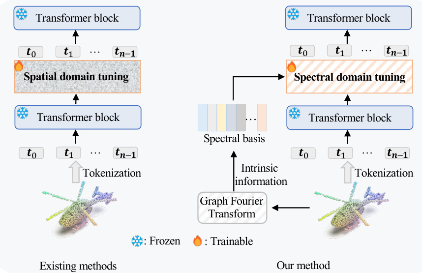
(a) The comparison between existing PEFT methods (left) and our method (right)
(a) 现有PEFT方法(左)与我们的方法(右)的对比
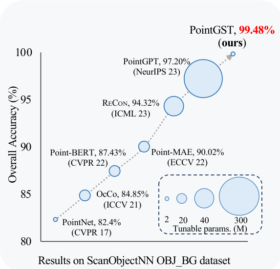
(b) The comparisons in terms of performance and trainable parameters Fig. 1: (a) The comparison of existing PEFT methods [88], [99] and our method. Instead of spatial tuning, we transform the point cloud to the spectral domain to mitigate the confusion among tokens and bring the intrinsic information of the downstream point clouds for targeted tuning. (b) The proposed PointGST outperforms all previous point cloud analysis methods while using extremely few trainable parameters. We even achieve a remarkable accuracy of $99.48%$ on the popular S can Object NN OBJ BG dataset, pushing the performance on this dataset to surpass $99%$ for the first time.
图 1: (a) 现有 PEFT 方法 [88], [99] 与我们方法的对比。我们不是进行空间调优,而是将点云转换到谱域,以减轻 Token 之间的混淆,并为下游点云带来内在信息进行针对性调优。(b) 所提出的 PointGST 在使用极少的可训练参数的情况下,优于所有先前的点云分析方法。我们甚至在流行的 Scan Object NN OBJ BG 数据集上实现了 $99.48%$ 的显著准确率,首次将该数据集的性能推至超过 $99%$。
Considering the above issues, we shift our focus to a new perspective: spectral domain fine-tuning. Spectral representations offer significant distinct ness over spatial domain representations. Specifically, compared to the spatial domain, features in the spectral domain can be easily decorrelated [57], [90], due to the ability of spectral representations to disentangle complex spatial relationships into distinct frequency components. This de correlation mitigates the confusion among tokens by using orthogonal components (spectral basis) to separate them. Additionally, the spectral basis obtained by the original point cloud offers direct intrinsic information about the downstream tasks to better guide the fine-tuning process. However, effectively and efficiently fine-tuning the parameters in the spectral domain is not a trivial problem, where two crucial concerns need to be considered: 1) what spectral transform to use, and 2) how to inject the intrinsic information into the fixed pretrained model by using this transform. An ideal transform for point clouds should be easy to construct, preserve intrinsic information, and adapt to the irregular structure of point cloud data. We find that the Graph Fourier Transform (GFT)
考虑到上述问题,我们将注意力转向一个新的视角:频域微调。频域表示在空间域表示上具有显著的独特性。具体来说,与空间域相比,频域中的特征可以轻松去相关 [57], [90],这是因为频域表示能够将复杂的空间关系分解为不同的频率分量。这种去相关通过使用正交分量(频谱基)来分离 token,从而减轻了 token 之间的混淆。此外,原始点云获得的频谱基提供了关于下游任务的直接内在信息,以更好地指导微调过程。然而,在频域中有效且高效地微调参数并非易事,其中需要考虑两个关键问题:1) 使用何种频谱变换,2) 如何通过使用这种变换将内在信息注入到固定的预训练模型中。对于点云来说,理想的变换应该易于构建、保留内在信息,并适应点云数据的不规则结构。我们发现图傅里叶变换 (Graph Fourier Transform, GFT)
stands out as particularly suitable. A properly constructed graph can provide a natural representation of the irregular point clouds that are adaptive to their structure, and the graph spectral domain can explicitly reveal geometric structures, from basic shapes to fine details, within a compressed space [25].
特别适合的是,一个适当构建的图可以提供一种自然的不规则点云表示,这种表示能够适应其结构,并且图谱域可以在压缩空间中明确揭示从基本形状到细节的几何结构 [25]。
In this paper, we explore the potential of fine-tuning parameters in the spectral domain. Our approach, illustrated in Fig. 1(a), introduces a novel PEFT method that optimizes a frozen pre-trained point cloud model through Graph Spectral Tuning, which we refer to as PointGST. Specifically, we first construct a series of multi-scale point cloud graphs that enable the calculation of global and local spectral basis, which will bring the intrinsic information like the geometry of the original point cloud. Then, we propose a lightweight Point Cloud Spectral Adapter (PCSA) to transform the point tokens (serving as graph signal) from the spatial domain to the spectral domain using the spectral basis. Based on the spectral point tokens, our PCSA adopts an effortless shared linear layer to adapt the global and local spectral tokens to meet the downstream tasks. In the spectral domain, adjusting parameters actually modifies the “energy” of each graph frequency for the graph signal, improving the de correlation of the inner confused tokens when transforming back to the spatial domain. Besides, the information of the generated spectral basis is inherently aware of the unique characteristics of the downstream point clouds, enabling targeted fine-tuning.
本文探讨了在频谱域中微调参数的潜力。我们的方法如图 1(a) 所示,引入了一种新颖的参数高效微调 (PEFT) 方法,通过图频谱调优 (Graph Spectral Tuning) 来优化冻结的预训练点云模型,我们称之为 PointGST。具体来说,我们首先构建了一系列多尺度点云图,使得能够计算全局和局部频谱基,这将带来原始点云的几何等内在信息。然后,我们提出了一种轻量级的点云频谱适配器 (Point Cloud Spectral Adapter, PCSA),使用频谱基将点 token(作为图信号)从空间域转换到频谱域。基于频谱点 token,我们的 PCSA 采用了一个简单的共享线性层来适应全局和局部频谱 token,以满足下游任务的需求。在频谱域中,调整参数实际上修改了图信号每个图频率的“能量”,从而在转换回空间域时改善了内部混淆 token 的去相关性。此外,生成的频谱基信息本质上了解下游点云的独特特征,从而实现有针对性的微调。
Extensive experiments conducted on challenging point cloud datasets across various tasks and data settings demonstrate the effectiveness of our PointGST. For example, when adopting the convincing Point-BERT [85] (resp., Point-MAE [40]) as the baseline, our approach archives notable performance improvement over fully fine-tuning by $3.96%$ , $1.55%$ , $2.57%$ , and $0.7%$ (resp., $1.72%$ $1.90%$ , $0.11%$ , and $0.3%$ ) on the S can Object NN OBJ BG, OBJ ONLY, PB T50 RS and ModelNet40 datasets, while surprisingly only requires about $2.77%$ of the total learnable parameters. More importantly, our method even boosts the largescale pre-trained models PointGPT-L [4], only using $0.6%$ trainable parameters to achieve $99.48%$ accuracy on the S can Object NN OBJ BG dataset, outperforming the SOTA method PointGPT-L [4] by $2.28%$ , establishing the new stateof-the-art. To the best of our knowledge, we are the first to push the performance on this dataset to surpass $99%$ . We also draw the intuitive trend of performance and trainable parameters in Fig. 1(b).
在各种任务和数据设置下,对具有挑战性的点云数据集进行的大量实验证明了我们的PointGST的有效性。例如,当采用令人信服的Point-BERT [85](或Point-MAE [40])作为基线时,我们的方法在完全微调的基础上实现了显著的性能提升,分别在S can Object NN OBJ BG、OBJ ONLY、PB T50 RS和ModelNet40数据集上提升了$3.96%$、$1.55%$、$2.57%$和$0.7%$(或$1.72%$、$1.90%$、$0.11%$和$0.3%$),而令人惊讶的是,仅需要约$2.77%$的总可学习参数。更重要的是,我们的方法甚至提升了大规模预训练模型PointGPT-L [4]的性能,仅使用$0.6%$的可训练参数就在S can Object NN OBJ BG数据集上达到了$99.48%$的准确率,比SOTA方法PointGPT-L [4]高出$2.28%$,建立了新的最先进水平。据我们所知,我们是第一个将该数据集的性能推至超过$99%$的团队。我们还在图1(b)中绘制了性能和可训练参数的直观趋势。
Our main contributions are summarized as follows: 1) In this paper, we propose a novel Parameter-Efficient FineTuning (PEFT) method for point cloud learning, named PointGST, which innovative ly fine-tunes parameters from a fresh perspective, i.e., spectral domain. 2) PointGST introduces the Point Cloud Spectral Adapter (PCSA) for frozen pre-trained backbones, transferring the inner confused tokens from the spatial domain into the spectral domain. It effectively mitigates the confusion among tokens and brings intrinsic information from downstream point clouds to meet the requirement of fine-tuned tasks. 3) Extensive experiments across various datasets demonstrate that our proposed method outperforms all current point cloudcustomized PEFT approaches. Remarkably, we achieve state-of-the-art performance on six challenging point cloud datasets while only using about $0.6%$ trainable parameters, serving as a promising option for fine-tuning the point cloud data.
我们的主要贡献总结如下:1) 本文提出了一种新颖的参数高效微调 (Parameter-Efficient FineTuning, PEFT) 方法,名为 PointGST,该方法从频谱域的全新视角创新性地微调参数。2) PointGST 引入了点云频谱适配器 (Point Cloud Spectral Adapter, PCSA),用于冻结预训练的主干网络,将空间域中混淆的 Token 转移到频谱域。它有效缓解了 Token 之间的混淆,并从下游点云中提取内在信息,以满足微调任务的需求。3) 在多个数据集上的广泛实验表明,我们提出的方法优于当前所有点云定制的 PEFT 方法。值得注意的是,我们在六个具有挑战性的点云数据集上实现了最先进的性能,同时仅使用了约 $0.6%$ 的可训练参数,为点云数据的微调提供了一个有前景的选择。
2 RELATED WORKS
2 相关工作
2.1 Point Cloud Learning
2.1 点云学习
Constructing structural representations for the point cloud has become a core topic in the computer vision community. To address the irregularity and sparsity of point clouds, the pioneering PointNet [48] adopts shared MLP layers to extract point features independently. The subsequent works further integrate local and global information [37], [49], [52], [56], [61], [72], self-attention mechanisms [19], [77], [78], [96], and various regular iz ation techniques [75], [92], [94], prompting the field.
构建点云的结构表示已成为计算机视觉领域的核心课题。为了解决点云的不规则性和稀疏性,开创性的 PointNet [48] 采用共享的 MLP 层独立提取点特征。后续工作进一步整合了局部和全局信息 [37]、[49]、[52]、[56]、[61]、[72],自注意力机制 [19]、[77]、[78]、[96],以及各种正则化技术 [75]、[92]、[94],推动了该领域的发展。
More recently, self-supervised pre-training methods [16], [36], [50], [81], [85], [98], have gained significant attention in the domain for their remarkable transfer capabilities by learning latent representations from unlabeled data and then fine-tuning on various downstream tasks. Point cloud pre-training approaches can be categorized into contrastbased [1], [6], [81] and reconstruct-based [4], [11], [47], [51], [85], [93] paradigms. In the contrast-based paradigm, Point Contrast [81] and CrossPoint [1] extract latent information from different views of the point cloud. Conversely, reconstruction-based methods involve randomly masking point clouds and then using auto encoders to reconstruct the original input. Among them, Point-BERT [85] learns by comparing masked encodings with outputs from a dVAEbased point cloud tokenizer. Point-MAE [47] and PointM2AE [93] reconstructs original point clouds via an autoencoder. Following this, PointGPT [4] leverages an extractorgenerator-based transformer as a GPT-style approach. To tackle data scarcity in 3D representation learning, interest in using cross-modal data for point cloud analysis is growing. For instance, ACT [11] trains 3D representation models using cross-modal pre-trained models as teachers, and RECON [50], [51] unifies reconstruction and cross-modal contrast modeling further.
最近,自监督预训练方法 [16], [36], [50], [81], [85], [98] 在领域中因其通过从未标记数据中学习潜在表示并在各种下游任务上进行微调的显著迁移能力而获得了广泛关注。点云预训练方法可以分为基于对比的 [1], [6], [81] 和基于重建的 [4], [11], [47], [51], [85], [93] 范式。在基于对比的范式中,Point Contrast [81] 和 CrossPoint [1] 从点云的不同视图中提取潜在信息。相反,基于重建的方法涉及随机掩码点云,然后使用自编码器重建原始输入。其中,Point-BERT [85] 通过比较掩码编码与基于 dVAE 的点云分词器的输出来进行学习。Point-MAE [47] 和 PointM2AE [93] 通过自编码器重建原始点云。随后,PointGPT [4] 利用基于提取器-生成器的 Transformer 作为 GPT 风格的方法。为了解决 3D 表示学习中的数据稀缺问题,使用跨模态数据进行点云分析的兴趣正在增长。例如,ACT [11] 使用跨模态预训练模型作为教师来训练 3D 表示模型,而 RECON [50], [51] 进一步统一了重建和跨模态对比建模。
Generally, these pre-training approaches typically transfer to the downstream 3D point cloud analysis tasks by fully fine-tuning the pre-trained models. However, as model parameters rapidly increase with scaling up [4], [51], fully fine-tuning incurs high tuning and storage costs and may dilute the pre-training knowledge. This paper seeks to reduce training costs through efficient transfer learning algorithms.
通常,这些预训练方法通过完全微调预训练模型来迁移到下游的3D点云分析任务。然而,随着模型参数随着规模的扩大而迅速增加 [4], [51],完全微调会带来高昂的调优和存储成本,并可能稀释预训练知识。本文旨在通过高效的迁移学习算法来降低训练成本。
2.2 Parameter-Efficient Fine-Tuning
2.2 参数高效微调
Parameter-Efficient Fine-Tuning (PEFT) aims to adopt a trainable module with a few parameters for fine-tuning. It has become a hot research topic in both the NLP [7], [10], [58], [62], [91] and computer vision [26], [35], [67], [86] communities. The mainstream PEFT methods can be roughly categorized into Adapter-based and Prompt-based.
参数高效微调 (Parameter-Efficient Fine-Tuning, PEFT) 旨在采用一个具有少量参数的可训练模块进行微调。它已成为自然语言处理 (NLP) [7], [10], [58], [62], [91] 和计算机视觉 [26], [35], [67], [86] 领域的热门研究课题。主流的 PEFT 方法大致可分为基于适配器 (Adapter-based) 和基于提示 (Prompt-based) 的方法。
Specifically, the Adapter-based [7], [23], [24], [33], [62] methods usually insert a trainable module between frozen modules to adjust the pre-trained models. Particularly, Adapt former [7] adds the adapter [23] in the FFN for the visual recognition tasks. The Prompt-based methods [26], [29], [34], [58] usually leverage the additional tokens (i.e., prompts) to the model input. For example, VPT [26], the first prompt-tuning method for vision tasks, prepends additional tunable tokens to the input or hidden layers of ViTs. Apart from paradigms mentioned above, some methods make new attempts, such as directly performing a linear transformation to modulate the features [35] or fine-tuning the bias term in each layer [86].
具体来说,基于适配器 (Adapter-based) [7], [23], [24], [33], [62] 的方法通常会在冻结模块之间插入一个可训练的模块,以调整预训练模型。特别是,Adapt former [7] 在 FFN 中添加了适配器 [23],用于视觉识别任务。基于提示 (Prompt-based) 的方法 [26], [29], [34], [58] 通常利用额外的 token(即提示)来调整模型输入。例如,VPT [26] 是第一个用于视觉任务的提示调优方法,它将额外的可调 token 添加到 ViT 的输入或隐藏层中。除了上述范式外,一些方法还进行了新的尝试,例如直接对特征进行线性变换以调整特征 [35],或微调每层中的偏置项 [86]。
Recently, some works [14], [15], [32], [60], [63], [64], [88], [99] attempt to explore the PEFT in point cloud tasks. As the earliest method, IDPT [88] applies DGCNN [74] to extract dynamic prompts for different instances instead of the traditional static prompts. Point-PEFT [64] attempts to aggregate local point information during fine-tuning. DA [15] introduces a dynamic aggregation strategy to replace previous static aggregation like mean or max pooling for pre-trained point cloud models. Recently, DAPT [99] proposes an approach combining the dynamic scale adapters with internal prompts as an efficient way of point cloud transfer learning. Although these methods can effectively reduce training costs, they are difficult to achieve the desired performance consistently and generalize poorly. We argue it is attributed to the limitation of fine-tuning in the spatial domain and lack of introducing strong intrinsic information of downstream point cloud. In contrast, we try to fine-tune the parameters in the spectral domain, which effectively mitigates the confusion among tokens and brings intrinsic information about downstream point clouds.
最近,一些工作 [14], [15], [32], [60], [63], [64], [88], [99] 尝试在点云任务中探索参数高效微调 (PEFT)。作为最早的方法,IDPT [88] 应用 DGCNN [74] 为不同实例提取动态提示,而不是传统的静态提示。Point-PEFT [64] 尝试在微调过程中聚合局部点信息。DA [15] 引入了一种动态聚合策略,以替代预训练点云模型中的静态聚合(如均值或最大池化)。最近,DAPT [99] 提出了一种结合动态尺度适配器和内部提示的方法,作为点云迁移学习的有效方式。尽管这些方法可以有效降低训练成本,但它们难以始终如一地达到预期性能,并且泛化能力较差。我们认为这归因于空间域微调的局限性以及缺乏引入下游点云的强内在信息。相比之下,我们尝试在频域中微调参数,这有效缓解了 token 之间的混淆,并带来了下游点云的内在信息。
2.3 Spectral Methods for Point Clouds
2.3 点云的谱方法
Methods that utilize spectral information to understand point clouds achieve notable advancements [5], [30], [43], [66]. For example, Wang et al. [71] combine spectral feature learning with recursive clustering to overcome the isolated local feature aggregation. Zhang et al. [95] introduce tensorbased methods to estimate hypergraph spectrum components and frequency coefficients of point clouds in both ideal and noisy settings. GSDA [39] proposes the graph spectral domain attack, perturbing graph transform coefficients in the spectral domain. Point Wavelet [76] designs graph wavelet transform to avoid the very time-consuming spectral decomposition. Ramasinghe et al. [54] propose a spectral-domain GAN that generates novel 3D shapes by using a spherical harmonics-based representation.
利用光谱信息理解点云的方法取得了显著进展 [5], [30], [43], [66]。例如,Wang 等人 [71] 将光谱特征学习与递归聚类相结合,以克服孤立的局部特征聚合问题。Zhang 等人 [95] 引入了基于张量的方法,用于在理想和噪声环境下估计点云的超图谱分量和频率系数。GSDA [39] 提出了图谱域攻击,通过在谱域中扰动图变换系数来实现攻击。Point Wavelet [76] 设计了图小波变换,以避免耗时的谱分解。Ramasinghe 等人 [54] 提出了一种谱域 GAN,通过使用基于球谐函数的表示来生成新颖的 3D 形状。
In this paper, we focus on the practical Parameterefficient Fine-Tuning (PEFT) task, and propose a fresh PEFT method named PointGST for point cloud tasks, which efficiently fine-tunes the given pre-trained point cloud models in the spectral domain. The fundamental goals and techniques between our method and previous spectral-based point cloud methods are different.
在本文中,我们专注于实用的参数高效微调 (Parameter-efficient Fine-Tuning, PEFT) 任务,并提出了一种名为 PointGST 的新 PEFT 方法,用于点云任务。该方法在频谱域中高效微调给定的预训练点云模型。我们的方法与之前基于频谱的点云方法在基本目标和技术上有所不同。
3 PRELIMINARY
This section revisits the mainstream fine-tuning paradigms and introduces the concept of Graph Fourier Transform.
3.1 Fine-Tuning Paradigm
Fully Fine-Tuning (FFT) is the most commonly used finetuning paradigm. Given a downstream training set $\mathbf{\Gamma}\mathbf{\Gamma}(\pmb{x};\pmb{y})$ ( $\boldsymbol{\mathbf{\rho}}_{x}$ is the input and $\pmb{y}$ is the label), the FFT trains the network $\mathcal{F}(\pmb{x};\pmb{\theta})$ and obtains the updated weight $\pmb{\theta}^{*}$ , where $\pmb{\theta}$ is the trainable parameters of $\mathcal{F}$ . Specifically, the FFT paradigm can be formulated as:
完全微调 (Fully Fine-Tuning, FFT) 是最常用的微调范式。给定一个下游训练集 $\mathbf{\Gamma}\mathbf{\Gamma}(\pmb{x};\pmb{y})$ (其中 $\boldsymbol{\mathbf{\rho}}_{x}$ 是输入,$\pmb{y}$ 是标签),FFT 训练网络 $\mathcal{F}(\pmb{x};\pmb{\theta})$ 并获得更新后的权重 $\pmb{\theta}^{*}$ ,其中 $\pmb{\theta}$ 是 $\mathcal{F}$ 的可训练参数。具体来说,FFT 范式可以表示为:

where $\ell$ represents the loss function for downstream tasks. Notably, the FFT updates $\pmb{\theta}$ to $\theta^{}$ , and $\theta^{}$ retains the same shape as $\pmb{\theta}$ after fine-tuning. In general, FFT will bring notable training costs reflected in GPU memory and storage.
其中 $\ell$ 表示下游任务的损失函数。值得注意的是,FFT 将 $\pmb{\theta}$ 更新为 $\theta^{}$,且 $\theta^{}$ 在微调后保持与 $\pmb{\theta}$ 相同的形状。通常,FFT 会带来显著的训练成本,体现在 GPU 内存和存储上。
Parameter-Efficient Fine-Tuning (PEFT) provides a practical solution by adapting pre-trained models to downstream tasks in a more efficient manner. Existing PEFT methods focus on tuning only a small subset of parameters $\theta^{\prime}$ . The optimized parameter $\tilde{\theta}^{\prime*}$ can be represented as:
参数高效微调 (Parameter-Efficient Fine-Tuning, PEFT) 提供了一种实用的解决方案,通过更高效的方式将预训练模型适配到下游任务。现有的 PEFT 方法专注于仅微调一小部分参数 $\theta^{\prime}$。优化后的参数 $\tilde{\theta}^{\prime*}$ 可以表示为:

The magnitude of $\left|\theta^{\prime*}\right|$ equals $\left|\theta^{\prime}\right|$ and is significantly smaller than the pre- trai ned $\pmb{\theta}$ . Du rin g fine-tuning, the pretrained $\pmb{\theta}$ remains fixed while only $\mathbf{\bar{\theta}}^{\prime}$ is update to $\mathbf{\hat{\theta}}^{\prime*}$ . Techniques for incorporating $\pmb{\theta}^{\prime}$ include adding lightweight additional parameters and selecting a small subset of the pre-trained $\pmb{\theta}$ .
$\left|\theta^{\prime*}\right|$ 的大小等于 $\left|\theta^{\prime}\right|$,并且明显小于预训练的 $\pmb{\theta}$。在微调过程中,预训练的 $\pmb{\theta}$ 保持不变,而只有 $\mathbf{\bar{\theta}}^{\prime}$ 被更新为 $\mathbf{\hat{\theta}}^{\prime*}$。引入 $\pmb{\theta}^{\prime}$ 的技术包括添加轻量级的额外参数和选择预训练 $\pmb{\theta}$ 的一小部分子集。
Adapter-like methods [7], [23], [84], adding lightweight extra parameters, are typical of the PEFT paradigm. Specifically, an Adapter-based approach usually includes a downsampling layer $W_{d}$ to reduce the feature dimension $C$ to $r,$ an activation function $\Phi.$ , and an up-sampling layer $W_{u}$ to recover the dimension. The low-rank dimension $r$ $(r\ll C)$ ) serves as a hyper-parameter for adapters. The formulation can be expressed as:
类似 Adapter 的方法 [7], [23], [84],通过添加轻量级的额外参数,是 PEFT 范式的典型代表。具体来说,基于 Adapter 的方法通常包括一个下采样层 $W_{d}$ 来将特征维度 $C$ 降低到 $r$,一个激活函数 $\Phi$,以及一个上采样层 $W_{u}$ 来恢复维度。低秩维度 $r$ $(r\ll C)$ 作为 Adapter 的超参数。其公式可以表示为:

where $\pmb{x}\in\mathbb{R}^{n\times C}$ represents the input vectors from a pretrained model. The output $\hat{\pmb x}$ is added back to the original computation graph, with multiple Adapter structures comprising the new parameters θ′.
其中 $\pmb{x}\in\mathbb{R}^{n\times C}$ 表示来自预训练模型的输入向量。输出 $\hat{\pmb x}$ 被添加回原始计算图中,多个 Adapter 结构组成了新的参数 θ′。
3.2 Graph Fourier Transform
3.2 图傅里叶变换
Let us define a graph $\mathcal{G}={\mathcal{V},\mathcal{E},\mathcal{W}}$ , where $\mathcal{G}$ is the set of vertices $(|{\mathcal{G}}|=n)$ ), $\mathcal{E}$ represents the edges, and $w$ is the adjacency matrix. In our context, a graph signal $z\in\mathbb{R}^{n\times c}$ assigns a vector $(\boldsymbol{z}{i}\in\mathbb{R}^{1\times c})$ ) to each vertex, while the entry $w{i,j}$ in $w$ indicates the weight of the edge between vertices $i$ and $j,$ reflecting their similarity. Then the Laplacian matrix is defined as $\pmb{L}=\pmb{D}-\pmb{\mathscr{W}}$ [59], where $_D$ is a diagonal matrix with each element $\begin{array}{r}{d_{i,i}\stackrel{_}{=}\sum_{j=0}^{n-1}w_{i,j}}\end{array}$ representing the degree of vertex $i$ . For an und irected graph with nonnegative weights, $\pmb{L}\in\mathbb{R}^{n\times n}$ is real, symmetric, and positive semi-definite [8]. This allows for the eigen-decomposition ${\pmb L}={\pmb U}{\pmb\Lambda}{\pmb U}^{\top}$ , where $\pmb{U}=[\mathbf{u}_{0},\dots,\mathbf{u}_{n-1}]$ is an orthonor- mal matrix composed of ei gen vectors $\mathbf{u}_{i},$ and eigenvalues $\mathbf{\Lambda}\mathbf{A}=\mathrm{diag}(\lambda_{0},\ldots,\lambda_{n-1})$ are often interpreted as the graph frequencies.
让我们定义一个图 $\mathcal{G}={\mathcal{V},\mathcal{E},\mathcal{W}}$,其中 $\mathcal{G}$ 是顶点集合 $(|{\mathcal{G}}|=n)$,$\mathcal{E}$ 表示边,$w$ 是邻接矩阵。在我们的上下文中,图信号 $z\in\mathbb{R}^{n\times c}$ 为每个顶点分配一个向量 $(\boldsymbol{z}{i}\in\mathbb{R}^{1\times c})$,而 $w$ 中的元素 $w{i,j}$ 表示顶点 $i$ 和 $j$ 之间边的权重,反映了它们的相似性。然后拉普拉斯矩阵定义为 $\pmb{L}=\pmb{D}-\pmb{\mathscr{W}}$ [59],其中 $_D$ 是一个对角矩阵,每个元素 $\begin{array}{r}{d_{i,i}\stackrel{_}{=}\sum_{j=0}^{n-1}w_{i,j}}\end{array}$ 表示顶点 $i$ 的度数。对于具有非负权重的无向图,$\pmb{L}\in\mathbb{R}^{n\times n}$ 是实对称且半正定的 [8]。这使得特征分解 ${\pmb L}={\pmb U}{\pmb\Lambda}{\pmb U}^{\top}$ 成为可能,其中 $\pmb{U}=[\mathbf{u}_{0},\dots,\mathbf{u}_{n-1}]$ 是由特征向量 $\mathbf{u}_{i}$ 组成的正交矩阵,特征值 $\mathbf{\Lambda}\mathbf{A}=\mathrm{diag}(\lambda_{0},\ldots,\lambda_{n-1})$ 通常被解释为图的频率。
Specifically, the ei gen vectors above can be viewed as a set of spectral basis, allowing the Graph Fourier Transform (GFT) of the graph signal $_{z}$ to be expressed as:
具体来说,上述特征向量可以视为一组谱基,使得图信号 $_{z}$ 的图傅里叶变换 (Graph Fourier Transform, GFT) 可以表示为:

where $\hat{\textbf{\textit{z}}}\in\mathbb{R}^{n\times c}$ represents the spectral coefficients for different graph frequencies, with the square of each column indicating the “energy” of the corresponding frequency. Similarly, the inverse Graph Fourier Transform (iGFT) is then defined as:
其中 $\hat{\textbf{\textit{z}}}\in\mathbb{R}^{n\times c}$ 表示不同图频率的频谱系数,每列的平方表示对应频率的“能量”。类似地,逆图傅里叶变换 (iGFT) 定义为:

In our method, we associate graph vertices with key points in the point cloud, constructing the adjacency matrix $w$ considering the distances among these points.
在我们的方法中,我们将图顶点与点云中的关键点关联起来,构建邻接矩阵 $w$,并考虑这些点之间的距离。
4 METHOD
4 方法
Fully fine-tuning a pre-trained point cloud model provides advanced performance, but substantial training costs accompany it. To address this challenge, we propose a novel method called PointGST, where the overall framework is illustrated in Fig. 2. Specifically, our method mainly consists of a regular pre-trained backbone and a series of lightweight Point Cloud Spectral Adapters (PCSA) integrated into each Transformer layer. During the fine-tuning, we keep the entire backbone frozen and only utilize a small number of trainable parameters (i.e., PCSA) to learn task-specific knowledge from the features of each instance. The PCSA transforms the point tokens from the spatial to the spectral domain, which de-correlates the inherent confusion of the point tokens from the frozen backbone. It efficiently finetunes fewer parameters for downstream tasks while introducing intrinsic information from the downstream point clouds for targeted tuning. As a result, it can significantly reduce the training cost and effectively connect the general knowledge from the pre-trained tasks with downstream tasks, leading to promising performance.
完全微调预训练的点云模型提供了先进的性能,但也伴随着巨大的训练成本。为了解决这一挑战,我们提出了一种名为 PointGST 的新方法,其整体框架如图 2 所示。具体来说,我们的方法主要由一个常规的预训练骨干网络和一系列轻量级的点云频谱适配器 (Point Cloud Spectral Adapters, PCSA) 组成,这些适配器集成到每个 Transformer 层中。在微调过程中,我们保持整个骨干网络冻结,仅利用少量可训练参数(即 PCSA)从每个实例的特征中学习任务特定的知识。PCSA 将点 Token 从空间域转换到频谱域,从而解除了冻结骨干网络中点 Token 的固有混淆。它有效地为下游任务微调了较少的参数,同时引入了来自下游点云的内在信息进行针对性调整。因此,它可以显著降低训练成本,并有效地将预训练任务中的通用知识与下游任务连接起来,从而实现出色的性能。
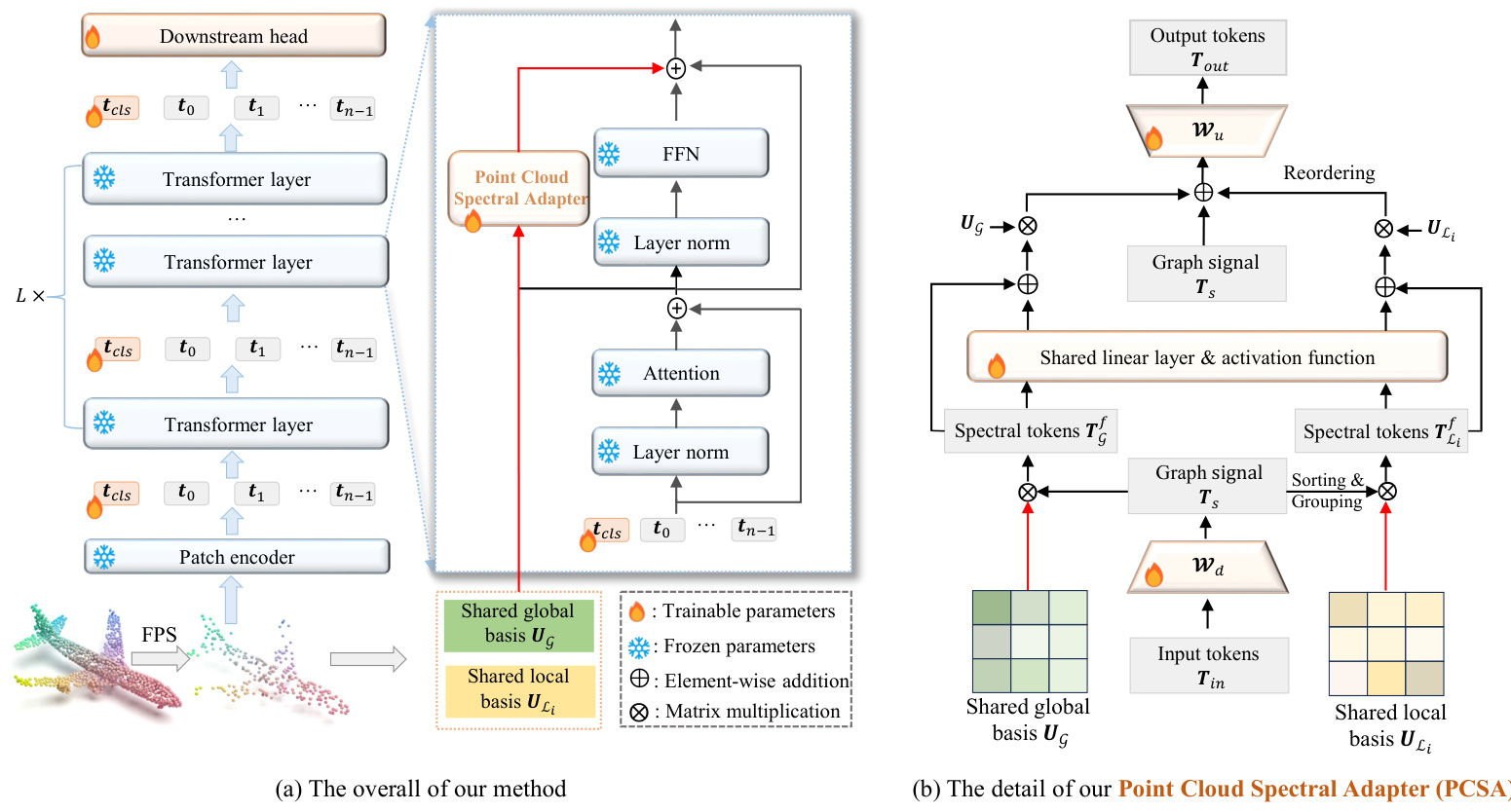
Fig. 2: (a) The overall of our PointGST. During the fine-tuning phase, we freeze the given pre-trained backbones and only fine-tune the proposed lightweight Point Cloud Spectral Adapter (PCSA). (b) The details of our proposed PCSA. We treat the point tokens as graph signals and then transfer the point tokens from the spatial domain to the spectral domain for tuning. The PCSA is injected into each transformer layer in a parallel paradigm.
图 2: (a) 我们的 PointGST 整体架构。在微调阶段,我们冻结给定的预训练骨干网络,仅微调提出的轻量级点云频谱适配器 (PCSA)。(b) 我们提出的 PCSA 的细节。我们将点 Token 视为图信号,然后将点 Token 从空间域转换到频谱域进行调优。PCSA 以并行范式注入到每个 Transformer 层中。
4.1 Transformer Encoder
4.1 Transformer 编码器
Due to its flexible s cal ability, the Transformer encoder has become the predominant backbone for pre-training in point cloud analysis [4], [11], [47], [50], [85]. Specifically, after pre-processing steps such as Farthest Point Sampling (FPS) and Grouping, a lightweight PointNet is used to generate a series of point tokens $({\check{t}{i}\in\mathbb{R}^{1\times d}\mid0\leq i\leq n-1})$ , where $d$ is the embedding dimension and $n$ indicates the number of point patches. A classification token $(\pmb{t}{c l s}\in\mathbb{R}^{1\times d})$ is then concatenated with these point tokens, forming $\mathbf{\delta}T_{0}~\in$ R(n+1)×d, which serves as the input to an L-layer Transformer. Each Transformer layer comprises an Attention module and a Feed-Forward Network (FFN), which are responsible for extracting token-to-token and channel-wise information, respectively:
由于其灵活的可扩展性,Transformer 编码器已成为点云分析中预训练的主要骨干网络 [4], [11], [47], [50], [85]。具体来说,在经过最远点采样 (FPS) 和分组等预处理步骤后,使用轻量级的 PointNet 生成一系列点 Token $({\check{t}{i}\in\mathbb{R}^{1\times d}\mid0\leq i\leq n-1})$,其中 $d$ 是嵌入维度,$n$ 表示点块的数量。然后,一个分类 Token $(\pmb{t}{c l s}\in\mathbb{R}^{1\times d})$ 与这些点 Token 拼接在一起,形成 $\mathbf{\delta}T_{0}~\in$ R(n+1)×d,作为 L 层 Transformer 的输入。每个 Transformer 层包含一个注意力模块和一个前馈网络 (FFN),分别负责提取 Token 到 Token 和通道级别的信息:

where T i R(n+1)×d represents the output of the $i$ -th layer, and LN denotes layer normalization. The Attention module and FFN are the most computationally and parameterintensive components of the Transformer. In our approach, we keep the entire Transformer encoder frozen and inject the proposed learnable Point Cloud Spectral Adapter (PCSA) into the FFN in a parallel configuration.
其中,$T_i \in \mathbb{R}^{(n+1) \times d}$ 表示第 $i$ 层的输出,LN 表示层归一化。Attention 模块和 FFN 是 Transformer 中计算量和参数量最大的部分。在我们的方法中,我们保持整个 Transformer 编码器冻结,并将提出的可学习点云频谱适配器 (PCSA) 以并行配置注入到 FFN 中。
4.2 Efficient Fine-Tuning in Spectral Domain
4.2 频谱域中的高效微调
Compared with the spatial domain, the point tokens in the spectral domain can be easily de-correlated by distinct frequency components. Fine-tuning the parameters in the spectral domain mitigates the confusion among tokens by using an orthogonal basis to separate them and provides compact intrinsic information from downstream point clouds. To achieve this, we introduce a simple and lightweight Point Cloud Spectral Adapter (PCSA) designed to learn taskspecific knowledge in the spectral domain, as illustrated in Fig. 2(b). The spectral fine-tuning process is as follows:
与空间域相比,频谱域中的点Token可以通过不同的频率分量轻松去相关。通过在频谱域中微调参数,使用正交基来分离Token,从而减轻Token之间的混淆,并从下游点云中提取紧凑的内在信息。为了实现这一点,我们引入了一个简单且轻量级的点云频谱适配器(Point Cloud Spectral Adapter, PCSA),旨在学习频谱域中的任务特定知识,如图 2(b) 所示。频谱微调过程如下:
In the following contents, we elaborately describe how to fine-tune the parameters in the spectral domain.
在以下内容中,我们将详细描述如何在频域中微调参数。
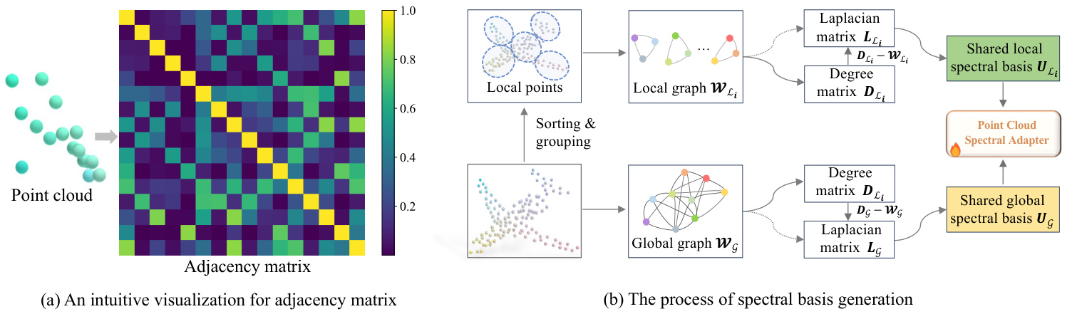
Fig. 3: (a) An intuitive visualization for our constructed graph, the adjacency matrix is symmetric, and the diagonal elements equal to 1. Smaller element values indicate greater geometric distances between point clouds. (b) The detailed process of our global and local spectral basis generation.
图 3: (a) 我们构建的图的直观可视化,邻接矩阵是对称的,对角线元素等于 1。元素值越小,表示点云之间的几何距离越大。(b) 我们全局和局部谱基生成的详细过程。
4.2.1 From Point Cloud to Graph
4.2.1 从点云到图
To implement spectral tuning, we first opt to convert the point cloud into a customized point graph $\mathcal{G}={\mathcal{V},\mathcal{E},\mathcal{W}}$ with vertices $\nu.$ , edges $\mathcal{E}$ and adjacency matrix $\boldsymbol{w}\in\mathbb{R}^{n\times n}$ . An ideal $\mathcal{G}$ should: 1) Contain $n$ vertices $(|\mathcal{V}|=n)$ representing the $n$ essential points in the point cloud. 2) The element $w_{i,j}$ in $w$ quantifies the relationship between $i$ -th and $j$ - th points, where the highest self-correlation is reflected by the diagonal element. 3) The relationship between points is influenced by their geometric properties, with closer point clouds exhibiting a stronger relationship.
为了实现光谱调谐,我们首先选择将点云转换为自定义的点图 $\mathcal{G}={\mathcal{V},\mathcal{E},\mathcal{W}}$,其中包含顶点 $\nu.$、边 $\mathcal{E}$ 和邻接矩阵 $\boldsymbol{w}\in\mathbb{R}^{n\times n}$。理想的 $\mathcal{G}$ 应满足以下条件:1) 包含 $n$ 个顶点 $(|\mathcal{V}|=n)$,代表点云中的 $n$ 个关键点。2) 矩阵 $w$ 中的元素 $w_{i,j}$ 量化了第 $i$ 个点和第 $j$ 个点之间的关系,其中对角线元素反映了最高的自相关性。3) 点之间的关系受其几何属性的影响,距离较近的点云表现出更强的关系。
Considering the design principles above, we calculate the relationship between the key points in a point patch. Then, we measure their pairwise distance to reflect the intrinsic information and capture the underlying structure. Specifically, we compute a point-pairwise distance matrix $\dot{\mathbf{\Delta}}\in\mathbb{R}^{n\times n},$ where each element $\delta_{i,j}\in\mathbb{R}$ represents the Euclidean distance between $i$ -th and $j$ -th points. However, such a distance matrix fails to meet principles 2) and 3), e.g., the distance from the $i$ -th point to itself is zero. Therefore, we further propose a simple data-dependent scaling strategy to define the adjacency matrix $w$ , and the element for $i$ -th row and $j$ -th column as follows:
考虑到上述设计原则,我们计算了点块中关键点之间的关系。然后,我们测量它们的成对距离以反映内在信息并捕捉底层结构。具体来说,我们计算了一个点对距离矩阵 $\dot{\mathbf{\Delta}}\in\mathbb{R}^{n\times n},$ 其中每个元素 $\delta_{i,j}\in\mathbb{R}$ 表示第 $i$ 个点和第 $j$ 个点之间的欧几里得距离。然而,这样的距离矩阵无法满足原则 2) 和 3),例如,第 $i$ 个点到自身的距离为零。因此,我们进一步提出了一种简单的数据依赖缩放策略来定义邻接矩阵 $w$,并将第 $i$ 行和第 $j$ 列的元素定义如下:

where $\operatorname*{min}(\Delta)=\operatorname*{min}(\delta_{i,j}),i\neq j$ represents the minimum value in $\Delta$ excluding zero, which varies across different samples and is data-dependent. $\b{I}\in\mathbb{R}^{n\times n}$ is an identity matrix. Using the geometric locations of key points and a data-dependent scaling strategy, we construct a graph with weights based on a distance metric between the points, incorporating all the desired properties. An intuitive visualization of our constructed graph for a point cloud is present in Fig. 3(a).
其中 $\operatorname*{min}(\Delta)=\operatorname*{min}(\delta_{i,j}),i\neq j$ 表示 $\Delta$ 中排除零的最小值,该值因样本而异且依赖于数据。$\b{I}\in\mathbb{R}^{n\times n}$ 是一个单位矩阵。通过使用关键点的几何位置和数据依赖的缩放策略,我们构建了一个基于点之间距离度量的加权图,并包含了所有期望的属性。图 3(a) 展示了我们为点云构建的图的直观可视化。
4.2.2 Multi-Scale Point Cloud Graphs
4.2.2 多尺度点云图
To comprehensively capture the underlying structure in point clouds, we generate a series of graphs that enable the calculation of both global and local ei gen vectors, as shown in Fig. 3(b). Such an approach ensures a thorough usage of spectral features across different scales.
为了全面捕捉点云中的底层结构,我们生成了一系列图,使得全局和局部特征向量的计算成为可能,如图 3(b) 所示。这种方法确保了在不同尺度上对频谱特征的充分利用。
Global graph. We first treat all key points as an entirety and transform them into a global graph2 $w_{g}$ . The details for translating the original point cloud to a graph are detailed in Sec. 4.2.1.
全局图。我们首先将所有关键点视为一个整体,并将它们转换为全局图2 $w_{g}$。将原始点云转换为图的详细信息详见第4.2.1节。
Local graph. We then propose constructing local subgraphs from neighboring point clouds to capture the local structure by rearranging the $n$ key points into $k$ groups along a particular pattern. To be specific, the original key point set ${p_{0},\cdots,p_{n-1}}$ is scanned and sorted into ${\dot{p_{0}^{\prime}},\dot{\cdot}\cdot\cdot,p_{n-1}^{\prime}}$ . This sorted set is then evenly divided into $k$ groups, with each group containing $m$ points, making $n=k\times m$ . The $i$ -th local point group can be defined as $\mathcal{L}_{i}=\left{p_{i m}^{\prime},\cdot\cdot\cdot,p_{\left(i+1\right)m-1}^{\prime}\mid0\leq i\leq k-1\right}$ . Based on this, we construct local sub-graphs for each group, resulting in $\left{\mathcal{W}_{\mathcal{L}_{0}},\cdot\cdot\cdot,\mathcal{W}_{\mathcal{L}_{i}},\cdot\cdot\cdot\tilde{\mathcal{W}_{\mathcal{L}_{k-1}}}\mid0\leq i\leq k-1\right}$ .
局部图。我们提出通过将 $n$ 个关键点按照特定模式重新排列成 $k$ 组,从邻近点云中构建局部子图以捕捉局部结构。具体来说,原始关键点集 ${p_{0},\cdots,p_{n-1}}$ 被扫描并排序为 ${\dot{p_{0}^{\prime}},\dot{\cdot}\cdot\cdot,p_{n-1}^{\prime}}$。然后,这个排序后的集合被均匀地分成 $k$ 组,每组包含 $m$ 个点,使得 $n=k\times m$。第 $i$ 个局部点组可以定义为 $\mathcal{L}_{i}=\left{p_{i m}^{\prime},\cdot\cdot\cdot,p_{\left(i+1\right)m-1}^{\prime}\mid0\leq i\leq k-1\right}$。基于此,我们为每组构建局部子图,得到 $\left{\mathcal{W}_{\mathcal{L}_{0}},\cdot\cdot\cdot,\mathcal{W}_{\mathcal{L}_{i}},\cdot\cdot\cdot\tilde{\mathcal{W}_{\mathcal{L}_{k-1}}}\mid0\leq i\leq k-1\right}$。
Both constructed global and local graphs effectively retain the intrinsic information of the original point cloud and underlying structure. These graphs subsequently will be used to generate the spectral basis, as detailed in the following subsection. Besides, the construction processing only needs to be implemented once for efficiency, i.e., the generated local and global graphs will be shared for all transformer layers.
构建的全局图和局部图都有效地保留了原始点云的内在信息和底层结构。这些图随后将用于生成谱基,如下一小节所述。此外,为了提高效率,构建过程只需执行一次,即生成的局部图和全局图将在所有Transformer层中共享。
4.2.3 Point Cloud Spectral Adapter
4.2.3 点云频谱适配器
The proposed Point Cloud Spectral Adapter (PCSA) aims to convert the point tokens from the spatial to the spectral domain, and then effectively fine-tune the transformed signal, as shown in Fig. 2(b). Our PCSA is simple and extremely lightweight, as it just contains two matrices used for dimension adjustment and one shared linear layer used to fine-tune the spectral point tokens.
提出的点云频谱适配器 (PCSA) 旨在将点 Token 从空间域转换到频谱域,然后有效地微调转换后的信号,如图 2(b) 所示。我们的 PCSA 非常简单且极其轻量,因为它仅包含用于维度调整的两个矩阵和一个用于微调频谱点 Token 的共享线性层。
Down-projection. Let us denote the input tokens as $\mathbf{\textit{T}}{i n}\in\mathbb{R}^{n\times C}$ , where $C$ is the input dimension. Here, we omit the class token and refer to ${\pmb T}{i n}$ as the $n$ point tokens in this section. Our PCSA begins with a downward projection using trainable parameters $\pmb{W}{d}\in\mathbb{R}^{r\times C}.$ , with $r\ll C$ . The low-rank graph signal $\pmb{T}{s}$ are obtained by:
下投影。我们将输入 Token 表示为 $\mathbf{\textit{T}}{i n}\in\mathbb{R}^{n\times C}$,其中 $C$ 是输入维度。这里我们省略了类别 Token,并将 ${\pmb T}{i n}$ 称为本节中的 $n$ 个点 Token。我们的 PCSA 从使用可训练参数 $\pmb{W}{d}\in\mathbb{R}^{r\times C}$ 的下投影开始,其中 $r\ll C$。低秩图信号 $\pmb{T}{s}$ 通过以下方式获得:

where $\pmb{T_{s}}\in\mathbb{R}^{n\times r}$ provides a general representation of point patches. The $n$ point patches are embedded by the corresponding $n$ key points with their neighbors, enabling $\pmb{T}{s}$ to function as a graph signal with the key points as vertices. The $\pmb{T}{s}$ is also rearranged into $k$ local graph signal, as mentioned in Sec. 4.2.2, resulting in $\mathbf{\Delta}T_{s}^{\mathcal{L}{i}}\in\mathbb{R}^{m\times r}(0\overset{\leftarrow}{\leq}i\leq k-1)$ , corresponding to the key points in $\mathcal{L}{i}$ . Also, the $\pmb{T}{s}$ can serve as the global graph signal notated as $\pmb{T}{s}^{\mathcal{G}}\in\mathbb{R}^{n\times r}$ .
其中 $\pmb{T_{s}}\in\mathbb{R}^{n\times r}$ 提供了点块的一般表示。$n$ 个点块通过对应的 $n$ 个关键点及其邻居嵌入,使得 $\pmb{T}{s}$ 可以作为以关键点为顶点的图信号。$\pmb{T}{s}$ 也被重新排列为 $k$ 个局部图信号,如第 4.2.2 节所述,得到 $\mathbf{\Delta}T_{s}^{\mathcal{L}{i}}\in\mathbb{R}^{m\times r}(0\overset{\leftarrow}{\leq}i\leq k-1)$,对应于 $\mathcal{L}{i}$ 中的关键点。此外,$\pmb{T}{s}$ 可以作为全局图信号,记为 $\pmb{T}{s}^{\mathcal{G}}\in\mathbb{R}^{n\times r}$。
Spectral basis generation. After the down-projection, the graph signal $\pmb{T}{s}$ still remains in the spatial domain. Two preparations are required before applying Graph Fourier Transform (GFT) in the spatial point clouds, first to compute the Laplacian matrix $\pmb{L{\mathcal{G}}}\in\bar{\mathbb{R}^{n\times n}}$ and $\pmb{L}{\mathcal{L}{i}}\in\mathbb{R}^{m\times m}$ for the constructed the global graph $\boldsymbol{\mathcal{W}}{\mathcal{G}}\in\mathbb{R}^{n\times n}$ and local sub-graphs $\pmb{\mathcal{W}}{\mathcal{L}_{i}}\in\mathbb{R}^{m\times m},$ , respectively. We then perform eigenvalue decomposition to generate the spectral basis for the GFT and its inverse, as shown in Fig. 3(b).
频谱基生成。在下投影之后,图信号 $\pmb{T}{s}$ 仍然保留在空间域中。在空间点云中应用图傅里叶变换 (Graph Fourier Transform, GFT) 之前,需要进行两项准备工作:首先计算全局图 $\boldsymbol{\mathcal{W}}{\mathcal{G}}\in\mathbb{R}^{n\times n}$ 和局部子图 $\pmb{\mathcal{W}}{\mathcal{L}{i}}\in\mathbb{R}^{m\times m}$ 的拉普拉斯矩阵 $\pmb{L_{\mathcal{G}}}\in\bar{\mathbb{R}^{n\times n}}$ 和 $\pmb{L}{\mathcal{L}{i}}\in\mathbb{R}^{m\times m}$。然后,我们执行特征值分解以生成 GFT 及其逆的频谱基,如图 3(b) 所示。
For simplicity, the following content uses the global spectral for illustration. Specifically, we first produce the diagonal degree matrix $D_{\mathcal{G}}$ for the global graph $w_{g}$ :
为简化起见,以下内容使用全局谱进行说明。具体来说,我们首先为全局图 $w_{g}$ 生成对角度矩阵 $D_{\mathcal{G}}$ :
where each entry $d_{i,i}$ indicates the sum of the weights on connected edges for each node (key point). Based on $D_{\mathcal{G}}$ , the graph Laplacian matrix is represented as $\pmb{L}{\mathcal{G}}=\pmb{D}{\mathcal{G}}-\pmb{\mathcal{W}}{\mathcal{G}}$ . The constructed graphs contain real and non-negative edge weights, making $\pmb{L}{\mathcal{G}}$ a real, symmetric, and positive semidefinite matrix [8]. Therefore, $\pmb{L}_{\mathcal{G}}$ can be decomposed as:
其中每个条目 $d_{i,i}$ 表示每个节点(关键点)上连接边的权重之和。基于 $D_{\mathcal{G}}$,图拉普拉斯矩阵表示为 $\pmb{L}{\mathcal{G}}=\pmb{D}{\mathcal{G}}-\pmb{\mathcal{W}}{\mathcal{G}}$。构建的图包含实数且非负的边权重,使得 $\pmb{L}{\mathcal{G}}$ 成为一个实对称半正定矩阵 [8]。因此,$\pmb{L}_{\mathcal{G}}$ 可以分解为:

where $U_{\mathcal{G}}=[\mathbf{u}{0},\cdot\cdot\cdot\mathbf{\mu},\mathbf{u}{n-1}]\in\mathbb{R}^{n\times n}$ is an orthogonal ma- trix of ei gen vectors $\mathbf{u}{i},$ formed as a set of spectral basis for spectral domain. Similarly, we can also obtain the Laplacian matrix $\pmb{L}{\mathcal{L}{i}}$ and $U{\mathcal{L}{i}}\in\mathbb{R}^{m\times m}$ for the local sub-graph $w{\mathscr{L}{i}}$ . The $U{\mathcal{G}}$ and $U_{\mathcal{L}_{i}}$ are computed only once and shared across all transformer layers.
其中 $U_{\mathcal{G}}=[\mathbf{u}{0},\cdot\cdot\cdot\mathbf{\mu},\mathbf{u}{n-1}]\in\mathbb{R}^{n\times n}$ 是一个由特征向量 $\mathbf{u}{i}$ 组成的正交矩阵,作为谱域的一组谱基。同样,我们也可以为局部子图 $w{\mathscr{L}{i}}$ 获得拉普拉斯矩阵 $\pmb{L}{\mathcal{L}{i}}$ 和 $U{\mathcal{L}{i}}\in\mathbb{R}^{m\times m}$。$U{\mathcal{G}}$ 和 $U_{\mathcal{L}_{i}}$ 只需计算一次,并在所有 Transformer 层中共享。
Graph Fourier Transform. We then perform a matrix multiplication of low-dimensional token (graph signal) $\pmb{T}{s}$ with spectral basis $U{\mathcal{G}}$ and $U_{\mathcal{L}{i}}$ to represent the graph signal in the spectral domain. Specifically, for the global graph signal $\pmb{T}{s},$ we apply GFT by multiplying it with the global basis $U_{\mathcal{G}}$ to output $\pmb{T}{\mathcal{G}}^{f}$ , derive global spectral information. SimilarGly, the $i\cdot$ -th locGal graph signal $\pmb{T}{s}^{\tilde{\mathcal{L}}{i}}$ will multiply with the local basis $U{\mathcal{L}{i}}$ , resulting in $\mathbf{\dot{\delta}}T{\mathcal{L}_{i}}^{f}$ :
图傅里叶变换。然后,我们将低维的Token(图信号)$\pmb{T}{s}$ 与频谱基 $U{\mathcal{G}}$ 和 $U_{\mathcal{L}{i}}$ 进行矩阵乘法,以在频域中表示图信号。具体来说,对于全局图信号 $\pmb{T}{s},$ 我们通过将其与全局基 $U_{\mathcal{G}}$ 相乘来应用GFT,输出 $\pmb{T}{\mathcal{G}}^{f}$,从而得到全局频谱信息。类似地,第 $i\cdot$ 个局部图信号 $\pmb{T}{s}^{\tilde{\mathcal{L}}{i}}$ 将与局部基 $U{\mathcal{L}{i}}$ 相乘,得到 $\mathbf{\dot{\delta}}T{\mathcal{L}_{i}}^{f}$ :

Next, all tokens are passed through a shared linear layer featuring a residual connection:
接下来,所有 Token 通过一个带有残差连接的共享线性层:

where the act refers to the Swish activation function [53]. We initialize the linear layer to zero during the initial stages for stable training.
其中 act 指的是 Swish 激活函数 [53]。我们在初始阶段将线性层初始化为零,以确保训练的稳定性。
Inverse Graph Fourier Transform. To align with the output of the transformer layer, these tuned tokens $\pmb{T}{\mathcal{L}{i}}^{f^{\prime}}$ and
逆图傅里叶变换。为了与Transformer层的输出对齐,这些调整后的Token $\pmb{T}{\mathcal{L}{i}}^{f^{\prime}}$ 和
$\pmb{T}_{\mathcal{G}}^{f^{\prime}}$ in the spectral domain will be further transformed back to the spatial domain via the inverse GFT (iGFT):
$\pmb{T}_{\mathcal{G}}^{f^{\prime}}$ 在频域中会通过逆图傅里叶变换 (iGFT) 进一步转换回空间域:

Iwt hsehroeu lbdo tbh $\hat{\boldsymbol{T}}{\mathcal{G}}^{f}$ teadn dt $\hat{\pmb T}{\mathcal L_{i}}^{f}$ d uaree t toh teh ce o in nv tre or td eu dc esdp astoiarlti tnogk eannsd. grouping strategy, the tokens of local spectral represent point cloud patches that do not align with the backbone part. Therefore, it is necessary to reorder the spatial local tokens to match the order of $\pmb{T}{s}$ . Specifically, we concatenate the T f of all sub-graphs and reordered it, resulting in the tokens $\hat{\boldsymbol{T}}{\mathcal{L}}^{f}\in\mathbb{R}^{n\times r}$ :
$\hat{\boldsymbol{T}}{\mathcal{G}}^{f}$ 和 $\hat{\pmb T}{\mathcal L_{i}}^{f}$ 分别表示全局和局部特征的分组策略。由于分组策略,局部光谱的 Token 表示的点云块与主干部分不对齐。因此,有必要重新排序空间局部 Token 以匹配 $\pmb{T}{s}$ 的顺序。具体来说,我们将所有子图的 T f 连接起来并重新排序,得到 Token $\hat{\boldsymbol{T}}{\mathcal{L}}^{f}\in\mathbb{R}^{n\times r}$:

Up-projection and output. The PCSA finally employs a zero-initialized upward projection matrix $\boldsymbol{W_{u}}\in\mathbb{R}^{C\times r}$ and a manual scale $s\in\mathbb R$ to restore the fine-tuned compressed representations to the dimensions processed by the backbone:
上投影与输出。PCSA 最终使用一个零初始化的上投影矩阵 $\boldsymbol{W_{u}}\in\mathbb{R}^{C\times r}$ 和一个手动缩放因子 $s\in\mathbb R$,将微调后的压缩表示恢复到骨干网络处理的维度:

where the output of the proposed point cloud spectral adapter $\mathbf{\delta}T_{o u t}$ is added back to the FFN of the transformer block, as shown in Fig. 2(a).
其中,所提出的点云频谱适配器输出 $\mathbf{\delta}T_{o u t}$ 被添加回 Transformer 模块的前馈网络 (FFN) 中,如图 2(a) 所示。
Through the PCSA, we successfully fine-tune the parameter in the spectral domain, effectively transferring the general knowledge to the downstream tasks.
通过 PCSA,我们成功地在频域中微调了参数,有效地将通用知识迁移到下游任务中。
4.3 Theoretical Analysis
4.3 理论分析
4.3.1 Insight of applying Graph Fourier Transform in PEFT
4.3.1 图傅里叶变换在PEFT中的应用洞察
We summarize applying Graph Fourier Transform in PEFT into twofold: 1) The Graph Fourier Transform (GFT) conducts a signal de correlation, resulting in a compact representation in the spectral domain. 2) Tuning in the spectral domain actually adjusts the “energy” of each graph frequency for the graph signal.
我们将图傅里叶变换 (Graph Fourier Transform, GFT) 在参数高效微调 (PEFT) 中的应用总结为两点:1) 图傅里叶变换对信号进行去相关操作,从而在频域中获得紧凑的表示。2) 在频域中进行调整实际上是在调整图信号中每个图频率的“能量”。
For discrete signals like point clouds, the graph Laplacian matrices can be considered as precision matrices within Gaussian-Markov Random Fields (GMRFs) [57]. This probabilistic perspective shows that the GFT approximates the Karhunen-Loeve Transform (KLT) for signal de correlation in GMRFs. Previous studies [12], [89], [90] also indicate that the GFT is an approximately optimal linear transform for decorrelating signals, which aids in geometric data compression. Since the GFT approximates the KLT for optimal signal de correlation across various statistical processes, tuning in this domain is efficient and explicit.
Besides, our method for generating customized point graphs considers the relationship between points and adapts to the topology of point clouds, thereby injecting intrinsic knowledge of downstream tasks into the GFT process. By adopting the GFT, we can define the $\alpha_{i}=\mathbf{u}{i}^{\top}\pmb{T},$ where $\mathbf{\dot{u}}{i}\in\mathbf{\hat{\mathbb{R}}}^{1\times\check{n}}$ is the $i$ -th ei gen vector and $\pmb{T}\in\mathbb{R}^{n\times r}$ is the graph signal. The term $\lvert\alpha_{i}\rvert^{2}$ is commonly referred to as the “energy” at the $i$ -th graph frequency (corresponding to the $k$ -th eigenvalue $\lambda_{i}$ of the Laplacian matrix) for signal $\mathbf{\delta}{\mathbf{{T}}}$ . In other words, the shared linear layer in the Point Cloud Spectral Adapter (PCSA) adjusts $\alpha{i}$ at each frequency, allowing our PointGST to implement a direct and effective fine-tuning paradigm.
TABLE 1: The comparison of our PointGST and baseline methods in terms of storage usage when fine-tuning various downstream point cloud datasets or tasks.
Based on the above perceptions, we argue that the proposed PCSA can supplement the inner informed features from the fixed branch with explicit knowledge directly from point clouds for better feature integration. Specifically, the downward project $W_{d}$ generates a low-ranked feature for each point patch, which acts as graph signals with key points as vertices. Additionally, the residual connection and zero-initialized strategy in our PCSA ensure training stability. The experiments in the following sections will validate the effectiveness and robustness of our architecture.
基于上述认知,我们认为所提出的PCSA能够通过点云直接补充固定分支的内部感知特征,实现更优的特征融合。具体而言,下投影 $W_{d}$ 会为每个点块生成低秩特征,这些特征作为以关键点为顶点的图信号。此外,PCSA中的残差连接与零初始化策略确保了训练稳定性。后续章节的实验将验证该架构的有效性与鲁棒性。
4.3.2 Training Cost
4.3.2 训练成本
Our method requires only fine-tuning the proposed lightweight Point Cloud Spectral Adapter (PCSA) while freezing the entire pre-trained backbone. Specifically, the GFT and iGFT operations do not introduce extra parameters, while each Spectral Adapter module adds only $2\times r\times d$ from $W_{d}/W_{u},$ and $r\times r$ from the shared tuning Linear as trainable parameters (bias and layer normalization are ignored). The intermediate dimension $r$ is relatively small compared to $d$ . For example, we only need to finetune about $0.6%$ of the parameters in the SOTA baseline, PointGPT-L [4], achieving promising results.
我们的方法仅需微调所提出的轻量级点云频谱适配器 (PCSA) ,同时冻结整个预训练主干网络。具体而言,GFT和iGFT操作不会引入额外参数,而每个频谱适配器模块仅从 $W_{d}/W_{u}$ 添加 $2\times r\times d$ 可训练参数,以及从共享调谐线性层添加 $r\times r$ 可训练参数 (偏置和层归一化被忽略) 。中间维度 $r$ 相对于 $d$ 较小。例如,我们仅需微调SOTA基准模型PointGPT-L [4] 中约 $0.6%$ 的参数,即可取得显著效果。
As the amount of downstream tasks or datasets requiring fine-tuning increases, we only need to store the task/dataset-specific PCSA and one original pre-trained models. As shown in Tab. 1, when fine-tuning various downstream tasks, our PointGST significantly compresses model size compared to the baselines (Point-MAE [47] and PointGPT-L [4]).
随着需要微调的下游任务或数据集数量增加,我们只需存储任务/数据集特定的PCSA和一个原始预训练模型。如表1所示,在对各种下游任务进行微调时,我们的PointGST相比基线方法(Point-MAE [47]和PointGPT-L [4])显著压缩了模型体积。
We further analyze the training GPU memory, which is an important metric for evaluating the training cost of a neural network. As shown in Fig. 4, our method significantly reduces training memory as the batch size increases compared with Point-MAE [47]. In addition, compared with the previous representative PEFT methods for point cloud [88], [99], we present clear advantages, especially under the widely-used batch sizes such as 16 and 32.
我们进一步分析了训练GPU内存,这是评估神经网络训练成本的重要指标。如图4所示,与Point-MAE [47]相比,随着批量大小的增加,我们的方法显著降低了训练内存。此外,与之前代表性的点云PEFT方法[88][99]相比,我们展现出明显优势,尤其是在16和32等常用批量大小下。
5 EXPERIMENTS SETUP
5 实验设置
This section describes the implementation details and the comparison methods.
本节介绍实现细节和对比方法。
5.1 Datasets and Implement Details
5.1 数据集与实现细节
All the experiments are conducted on a single NVIDIA 3090 GPU. During fine-tuning, the parameters of the pretrained backbones remain frozen, while only the newly added parameters are updated. The hyper-parameters $k$ and $r$ are set to 4 and 36, respectively. We employ a transpose format of $Z$ space-filling curve [46] to scan the key points to construct the local graphs. This subsection introduces the implementation details along with the dataset.
所有实验均在单张NVIDIA 3090 GPU上进行。微调过程中,预训练骨干网络的参数保持冻结,仅更新新增参数。超参数$k$和$r$分别设为4和36。我们采用$Z$空间填充曲线[46]的转置格式扫描关键点以构建局部图。本小节将介绍实现细节及数据集。
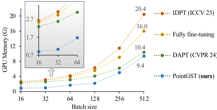
Fig. 4: The comparison of used training GPU memory.
图 4: 训练 GPU 显存使用量对比
S can Object NN [68] is a challenging 3D real-world objects dataset, consisting of ${\sim}15\mathrm{K}$ indoor object point cloud instances, across 15 categories. There are three widely used variants, including OBJ BG, OBJ ONLY, and PB T50 RS, each with increasing complexity. The training setup is aligned with the compared baseline. Specifically, we employ the AdamW optimizer [41] with a weight decay of 0.05 and a cosine learning rate scheduler [42], starting with an initial learning rate of 5e-4 and a 10-epoch warm-up. The model is trained for 300 epochs with a batch size of 32. For consistency, we utilize 2048 points in the point cloud, divided into 128 groups of 32 points each.
ScanObjectNN [68] 是一个具有挑战性的3D真实物体数据集,包含约15K个室内物体点云实例,涵盖15个类别。该数据集有三个广泛使用的变体,包括OBJ_BG、OBJ_ONLY和PB_T50_RS,每种变体的复杂度依次递增。训练设置与对比基线保持一致。具体而言,我们采用AdamW优化器 [41],权重衰减为0.05,并配合余弦学习率调度器 [42],初始学习率为5e-4,预热10个周期。模型训练共300个周期,批次大小为32。为保证一致性,我们使用2048个点云点,并将其分为128组,每组32个点。
ModelNet40 [79] is a commonly used synthesis 3D point cloud dataset that contains 12,311 CAD models of 40 categories. The network training settings follow S can Object NN. The input point cloud consists of 1,024 points, divided into 64 groups with 32 points per group.
ModelNet40 [79] 是一个常用的合成3D点云数据集,包含40个类别的12,311个CAD模型。网络训练设置遵循ScanObjectNN。输入点云由1,024个点组成,分为64组,每组32个点。
Shape Net part [83] is a popular point-level synthetic object part segmentation benchmark that includes 16,881 instances across 16 object categories and 50 part categories. We use the AdamW optimizer with a weight decay of 1e4 and the cosine learning rate scheduler, with an initial learning rate of 1e-4 and a 10-epoch warm-up. The models are trained for 300 epochs with a batch size of 16, using 2048 input points divided into 128 groups of 32 points each.
Shape Net部件数据集 [83] 是一个流行的点级别合成物体部件分割基准,包含16个物体类别和50个部件类别下的16,881个实例。我们使用AdamW优化器(权重衰减1e4)和余弦学习率调度器(初始学习率1e-4,10轮预热),以16的批次大小训练300轮,输入点数为2048个(分为128组,每组32个点)。
S3DIS [2] comprises six large-scale indoor areas, covering 273 million points from 13 categories. Following previous work [65], we advocate using Area 5 for evaluation purposes for better and fair generalization performance benchmarking. The cosine learning rate scheduler with an initial learning rate of 2e-4 is applied. We train our model for 60 epochs with a batch size of 32. Other configurations are the same as Shape Net part.
S3DIS [2] 包含六个大型室内区域,涵盖13个类别的2.73亿个点。遵循先前工作 [65],我们建议使用Area 5进行评估,以获得更好且公平的泛化性能基准测试。采用初始学习率为2e-4的余弦学习率调度器。我们以批量大小32训练模型60个周期。其他配置与Shape Net部分相同。
TABLE 2: The comparison between other fine-tuning strategies and our PointGST. We report the overall accuracy (OA) and trainable parameters (Params.) across three variants of S can Object NN [68] and ModelNet40 [79]. All methods use default data augmentation as the baseline. ∗ indicates reproduced results. S can Object NN results are reported without voting, while ModelNet40 results are presented both with and without voting $\left(-/-\right)$ .
表 2: 其他微调策略与我们的 PointGST 对比。我们报告了 S can Object NN [68] 和 ModelNet40 [79] 三个变体的总体准确率 (OA) 和可训练参数量 (Params.)。所有方法均使用默认数据增强作为基线。∗ 表示复现结果。S can Object NN 结果报告时不使用投票,而 ModelNet40 结果同时报告使用和不使用投票的情况 $\left(-/-\right)$。
| 预训练模型 | 微调策略 | 参考文献 | 参数量 (M) | FLOPs (G) | ScanObjectNN | ModelNet40 | ||
|---|---|---|---|---|---|---|---|---|
| OBJ_BG | OBJ_ONLY | PB_T50_RS | OA (%) | |||||
| Point-BERT [85] (CVPR 22) | 全微调 | 22.1 (100%) | 4.76 | 87.43 | 88.12 | |||
| IDPT [88] | ICCV 23 | 1.7 (7.69%) | 7.10 | 88.12(+0.69) | 88.30(+0.18) | 83.69(+0.62) | ||
| Point-PEFT [64] | AAAI 24 | 0.7 (3.13%) | 85.00(+1.93) | |||||
| DAPT [99] | CVPR 24 | 1.1 (4.97%) | 4.96 | 91.05(+3.62) | 89.67(+1.55) | 85.43(+2.36) | ||
| PointGST (ours) | 0.6 (2.77%) | 4.81 | 91.39(+3.96) | 89.67(+1.55) | 85.64(+2.57) | |||
| Point-MAE [47] (ECCV 22) | 全微调 | 22.1 (100%) | 4.76 | 90.02 | 88.29 | |||
| IDPT [88] | ICCV 23 | 1.7 (7.69%) | 7.10 | 91.22(+1.20) | 90.02(+1.73) | 84.94(-0.24) | ||
| DAPT [99] | CVPR 24 | 1.1 (4.97%) | 4.96 | 90.88(+0.86) | 90.19(+1.90) | 85.08(-0.10) | ||
| PointGST (ours) | 0.6 (2.77%) | 4.81 | 91.74(+1.72) | 90.19(+1.90) | 85.29(+0.11) | |||
| ACT [11] (ICLR 23) | 全微调 | 22.1 (100%) | 4.76 | 93.29 | 91.91 | 88.21 | ||
| IDPT [88] | ICCV 23 | 1.7 (7.69%) | 7.10 | 93.12(-0.17) | 92.26(+0.35) | 87.65(-0.56) | ||
| DAPT*[99] | CVPR 24 | 1.1 (4.97%) | 4.96 | 92.60(-0.69) | 91.57(-0.34) | 87.54(-0.67) | ||
| PointGST (ours) | - | 0.6 (2.77%) | 4.81 | 93.46(+0.17) | 92.60(+0.69) | 88.27(+0.06) | ||
| RECON [50] (ICML 23) | 全微调 | 22.1 (100%) | 4.76 | 94.32 | 92.77 | 90.01 | ||
| IDPT* [88] | ICCV 23 | 1.7 (7.69%) | 7.10 | 93.29(-1.03) | 91.57(-1.20) | 87.27(-2.74) | ||
| DAPT [99] | CVPR 24 | 1.1 (4.97%) | 4.96 | 94.32(-0.00) | 92.43(-0.34) | 89.38(-0.63) | ||
| PointGST (ours) | 0.6 (2.77%) | 4.81 | 94.49(+0.17) | 92.94(+0.17) | 89.49(-0.52) | |||
| PointGPT-L [4] (NeurIPS 23) | 全微调 | 360.5 (100%) | 67.71 | 97.2 | 96.6 | |||
| IDPT* [88] | ICCV 23 | 10.0 (2.77%) | 75.19 | 98.11(+0.91) | 96.04(-0.56) | 92.99(-0.41) | ||
| DAPT* [99] | CVPR 24 | 4.2 (1.17%) | 71.64 | 98.11(+0.91) | 96.21(-0.39) | 93.02(-0.38) | ||
| PointGST (ours) | 2.4 (0.67%) | 67.95 | 98.97(+1.77) | 97.59(+0.99) | 94.83(+1.43) |
5.2 Compared Methods
5.2 对比方法
To illustrate the effectiveness of our approach, popular pre-train models like Point-BERT [85], Point-MAE [47], ACT [11], RECON [50], and PointGPT [4] are selected as our baselines. Additionally, we include the SOTA point cloud PEFT methods for comparisons: 1) IDPT [88] utilizes DGCNN [74] to generate instance-aware prompts before the last transformer layer for model fine-tuning rather than relying on static prompts; 2) Point-PEFT [64] utilize a point-prior bank for feature aggregation and incorporating Adapters into each transformer block. 3) DA [15] uses a dynamic aggregation method to replace previous static aggregation for pre-trained point cloud Transformers. 4) DAPT [99], the latest SOTA point cloud PEFT method, proposes to adjust tokens based on significance scores.
为验证本方法的有效性,我们选取了Point-BERT [85]、Point-MAE [47]、ACT [11]、RECON [50]和PointGPT [4]等主流预训练模型作为基线。同时引入当前最先进的点云参数高效微调(PEFT)方法进行对比:1) IDPT [88] 采用DGCNN [74]在最后一层Transformer前生成实例感知提示,替代静态提示进行模型微调;2) Point-PEFT [64] 通过点特征先验库实现特征聚合,并在每个Transformer块中嵌入适配器;3) DA [15] 采用动态聚合方法替代预训练点云Transformer原有的静态聚合机制;4) 最新SOTA点云PEFT方法DAPT [99] 提出基于显著性分数调整Token的策略。
It is important to note that among the methods mentioned above, IDPT and DAPT conduct more comprehensive experiments compared to the other two approaches. As a result, we primarily follow the experimental setups of IDPT and DAPT to organize our experiments.
需要注意的是,在上述方法中,IDPT和DAPT相比其他两种方法进行了更全面的实验。因此,我们主要遵循IDPT和DAPT的实验设置来组织实验。
6 RESULTS AND ANALYSIS
6 结果与分析
In this section, we conduct experiments to show the effectiveness of our approach.
在本节中,我们通过实验验证所提方法的有效性。
TABLE 3: Classification on S can Object NN PB T50 RS [68] with strong data augmentation. Overall accuracy $(%)$ without voting is reported. Params. is the trainable parameters.
表 3: 在 S can Object NN PB T50 RS [68] 上的分类结果,采用强数据增强。报告了未使用投票的总体准确率 $(%)$。Params. 表示可训练参数量。
| 预训练模型 | 微调策略 | 引用 | Params. (M) | PB_T50_RS |
|---|---|---|---|---|
| Point-MAE [40] (ECCV 22) | Fully f fine-tune | 22.1 | 88.4 | |
| DA [15] | ICRA24 | 1.6 | 88.0 | |
| Point-PEFT [64] | AAAI 24 | 0.7 | 89.1 | |
| PointGST (ours) | 0.6 | 89.3 |
6.1 3D Classification
6.1 3D分类
6.1.1 The comparisons of different fine-tuning strategies
6.1.1 不同微调策略的比较
We first comprehensively compare the representative finetuning strategies used in the point cloud tasks, including the fully fine-tuning (FFT), IDPT [88], and DAPT [99], in terms of trainable parameters (Params.) and performance. We apply our PointGST to various pre-trained models, such as Point-BERT [85], Point-MAE [47], ACT [11], RECON [50], and PointGPT-L [4], size ranging from 22.1M to $360.5\mathrm{M}$ . Tab. 2 lists the detailed results, and it can find that:
我们首先全面比较了点云任务中使用的代表性微调策略,包括全参数微调 (FFT)、IDPT [88] 和 DAPT [99],从可训练参数量 (Params.) 和性能两个维度进行评估。我们将 PointGST 应用于多种预训练模型,如 Point-BERT [85]、Point-MAE [47]、ACT [11]、RECON [50] 和 PointGPT-L [4],模型规模从 22.1M 到 $360.5\mathrm{M}$ 不等。表 2 列出了详细结果,可以发现:
- PointGST effectively balances the number of trainable parameters and performance. Based on the quantitative comparisons, it is evident that increasing the scale of a pre-trained model will improve the performance. However, this would meanwhile come at a huge cost of fine-tuning, e.g., Point-MAE and PointGPT-L report $85.18%$ and $93.4%$ with 22.1M and 360.5M parameters on the S can Object NN PB T50 RS dataset, respectively. Thanks to only fine-tuning a few parameters in the spectral domain, our method can effectively address this dilemma. Specifically, on the most convincing pre-trained point cloud models, PointGPT-L, compared with the fully fine-tuning (FFT), we only need 2.4M trainable parameters, which is merely $0.6%$ of the FFT. More importantly, with so few training parameters, we even outperform the FFT by $1.77%$ , $0.99%$ , $1.43%$ , and $0.7%$ on the OBJ BG, OBJ OBLY, PB T50 RS and ModelNet40 datasets, respectively.
- PointGST 在可训练参数量和性能之间实现了有效平衡。定量对比表明,增大预训练模型规模确实能提升性能,但这会带来高昂的微调成本。例如 Point-MAE 和 PointGPT-L 在 S can Object NN PB T50 RS 数据集上分别以 2210 万和 3.605 亿参数取得了 85.18% 和 93.4% 的准确率。得益于仅需在频域微调少量参数,我们的方法成功解决了这一困境。具体而言,在最具说服力的预训练点云模型 PointGPT-L 上,相比全参数微调 (FFT),我们仅需 240 万可训练参数,仅为 FFT 的 0.6%。更重要的是,凭借如此少的训练参数,我们在 OBJ BG、OBJ OBLY、PB T50 RS 和 ModelNet40 数据集上分别以 1.77%、0.99%、1.43% 和 0.7% 的优势超越了 FFT 的表现。
10 TABLE 4: Comparison of overall accuracy (OA) and trainable parameters (Params.) across three variants of ScanObjectNN [68] and ModelNet40 [79]. Results highlighted in green indicate the use of the voting strategy.
表 4: ScanObjectNN [68] 和 ModelNet40 [79] 三个变体的总体准确率 (OA) 和可训练参数 (Params.) 对比。绿色高亮结果表示使用了投票策略。
| 方法 | 参考文献 | Params. (M) | ScanObjectNN | ModelNet40 | |||
|---|---|---|---|---|---|---|---|
| OBJ_BG | OBJ_ONLY | PB_T50_RS | Points Num. | OA (%) | |||
| 仅监督学习 | |||||||
| PointNet [48] | CVPR 17 | 3.5 | 73.3 | 79.2 | 68.0 | 1k | 89.2 |
| PointNet++ [49] | NeurIPS 17 | 1.5 | 82.3 | 84.3 | 77.9 | 1k | 90.7 |
| DGCNN [74] | TOG 19 | 1.8 | 82.8 | 86.2 | 78.1 | 1k | 92.9 |
| MVTN [20] | ICCV 21 | 11.2 | 82.8 | 1k | 93.8 | ||
| 3D-GCN [38] | TPAMI 22 | 1k | 92.1 | ||||
| RepSurf-U [55] | CVPR 22 | 1.5 | 84.3 | 1k | 94.4 | ||
| PointNeXt [52] | NeurIPS 22 | 1.4 | 87.7 | 1k | 94.0 | ||
| PTv2 [78] | NeurIPS 22 | 12.8 | 1k | 94.2 | |||
| PointMLP [44] | ICLR 22 | 13.2 | 85.4 | 1k | 94.5 | ||
| PointMeta [37] | CVPR 23 | 87.9 | |||||
| ADS [22] | ICCV 23 | 87.5 | 1k | 95.1 | |||
| X-3D [61] | CVPR 24 | 5.4 | 90.7 | ||||
| GPSFormer [72] | ECCV 24 | 2.4 | 95.4 | 1k | 94.2 | ||
| 自监督表征学习 (全微调) | |||||||
| OcCo [73] | ICCV 21 | 22.1 | 84.85 | 85.54 | 78.79 | 1k | 92.1 |
| Point-BERT [85] | CVPR 22 | 22.1 | 87.43 | 88.12 | 83.07 | 1k | 93.2 |
| MaskPoint [40] | ECCV 22 | 22.1 | 89.70 | 89.30 | 84.60 | 1k | 93.8 |
| Point-MAE [47] | ECCV 22 | 22.1 | 90.02 | 88.29 | 85.18 | 1k | 93.8 |
| Point-M2AE [93] | NeurIPS 22 | 15.3 | 91.22 | 88.81 | 86.43 | 1k | 94.0 |
| ACT [11] | ICLR 23 | 22.1 | 93.29 | 91.91 | 88.21 | 1k | 93.7 |
| RECON [50] | ICML 23 | 43.6 | 94.15 | 93.12 | 89.73 | 1k | 93.9 |
| PointGPT-L [4] | NeurIPS 23 | 360.5 | 97.2 | 96.6 | 93.4 | 1k | 94.7 |
| Point-FEMAE[87] | AAAI24 | 27.4 | 95.18 | 93.29 | 90.22 | 1k | 94.5 |
| P2P++ [75] | TPAMI 24 | 16.1 | 90.3 | 1k | 94.1 | ||
| PointDif [98] | CVPR 24 | 93.29 | 91.91 | 87.61 | |||
| PointMamba [36] | NeurIPS 24 | 12.3 | 94.32 | 92.60 | 89.31 | ||
| MH-PH [16] | ECCV 24 | 97.4 | 96.8 | 93.8 | 1k | 94.6 | |
| RECON++-L [51] | ECCV 24 | 657.2 | 98.80 | 97.59 | 95.25 | 1k | 94.8 |
| 自监督表征学习 (高效微调) | |||||||
| PointGST (ours) | 2.4 | 98.97 | 97.59 | 94.83 | 1k | 94.8 | |
| PointGST (ours) | 2.4 | 99.48 | 97.76 | 96.18 | 1k | 95.3 |
Compared to spatial domain-based methods like IDPT and DAPT, our PointGST achieves superior performance with fewer trainable parameters by leveraging the spectral domain, where features are more easily de-correlated. In addition, our PointGST introduces intrinsic information via the Graph Fourier Transform (GFT), enabling targeted finetuning. In short, PointGST proves to be a potential candidate that brings promising performance and parameter-efficient approaches to low-resource scenarios.
与基于空间域的方法(如IDPT和DAPT)相比,我们的PointGST通过利用谱域(其中特征更易解耦)以更少的可训练参数实现了更优性能。此外,PointGST通过图傅里叶变换 (GFT) 引入内在信息,从而实现针对性微调。简而言之,PointGST被证明是一种潜力方案,能为低资源场景带来优异性能与参数高效的方法。
- PointGST can effectively generalize to diverse pretrained models. A good PEFT method should consistently perform well across different pre-trained models, regardless of the pre-training strategies, data used, or model sizes. However, our observations reveal that existing PEFT methods [15], [64], [88], [99] fail to deliver consistent improvements across diverse pre-trained models. For instance, as shown in Tab. 2, we apply five distinct pre-trained models, varying in pre-training techniques (e.g., masked modeling and contrastive learning) and sizes (ranging from 22.1M to 360.5M parameters). Notably, both IDPT and DAPT exhibit negative impacts when applied to baselines like ACT and RECON. Even in scenarios where these methods produce positive outcomes, the gains from IDPT and DAPT remain limited. In contrast, our PointGST consistently yields improvements across most conducted pre-trained models and outperforms IDPT and DAPT.
- PointGST能有效泛化到不同的预训练模型。一个好的PEFT方法应在各种预训练模型上表现稳定,无论其预训练策略、数据或模型规模如何。但我们发现现有PEFT方法[15][64][88][99]无法在不同预训练模型上实现一致改进。如表2所示,我们测试了五种预训练模型,其预训练技术(如掩码建模和对比学习)和参数量(从22.1M到360.5M)各不相同。值得注意的是,IDPT和DAPT在应用于ACT和RECON等基线时会产生负面影响。即使这些方法产生正向结果时,其增益也十分有限。相比之下,我们的PointGST在大多数测试的预训练模型上都能稳定提升性能,且优于IDPT和DAPT。
In addition, we find that both Point-PEFT [64] and DA [15] apply the point cloud rotation as the data augmentation [11] on the Point-MAE. To keep fair, we also adopt the augmentations to conduct experiments. The comparisons in Tab. 3 clearly show that PointGST consistently achieves higher accuracy than Point-PEFT and DA.
此外,我们发现Point-PEFT [64]和DA [15]都在Point-MAE上采用了点云旋转作为数据增强[11]。为保持公平,我们也采用相同增强策略进行实验。表3中的对比清晰表明,PointGST始终比Point-PEFT和DA获得更高准确率。
6.1.2 Compared with state-of-the-art methods
6.1.2 与最先进方法的对比
The comparisons between the state-of-the-art (SOTA) methods and our proposed method on S can Object NN and ModelNet40 are illustrated in Tab. 4. We categorize the comparison methods into two types: supervised learning only and self-supervised representation learning with full finetuning. The results yield two notable observations regarding the efficacy of the proposed PointGST:
在S can Object NN和ModelNet40数据集上,现有最优方法(SOTA)与我们提出方法的对比如表4所示。我们将对比方法分为两类:纯监督学习和带全微调的自监督表征学习。实验结果揭示了关于PointGST有效性的两个重要发现:

Fig. 5: Few-shot training performance on the S can Object NN PB T50 RS dataset at different training data proportions.
图 5: S can Object NN PB T50 RS 数据集在不同训练数据比例下的少样本训练性能。
- Self-supervised representation learning methods [4], [11], [50] generally outperform those based solely on supervised learning [22], [44], [55], emphasizing the critical role of pre-training. Additionally, these self-supervised methods often involve more trainable parameters than their supervised counterparts (e.g., 13.2M and 657.2M for PointMLP [44] and $\mathrm{RECON{++-L}}$ [51], respectively), which underscores the practical relevance of parameter-efficient fine-tuning.
- 自监督表示学习方法 [4]、[11]、[50] 通常优于仅基于监督学习的方法 [22]、[44]、[55],这凸显了预训练的关键作用。此外,这些自监督方法通常比监督方法包含更多可训练参数 (例如 PointMLP [44] 和 $\mathrm{RECON{++-L}}$ [51] 分别有 13.2M 和 657.2M 参数),这进一步说明了参数高效微调的实际意义。
- When using PointGPT-L [4] as the baseline, our PointGST outperforms all previous methods, establishing a new state-of-the-art, while requiring only 2.4M trainable parameters. To the best of our knowledge, this is the first approach to nearly saturate the performance on the ScanObjectNN OBJ BG dataset (e.g., $99.48%$ OA). Note that it is not something that can be brought about by simply fitting a dataset. Instead, it highlights the current limitations of existing point cloud analysis datasets in effectively evaluating new methods. Consequently, we encourage the community to develop more challenging datasets to better assess the progress in future point cloud analysis research.
- 当以PointGPT-L [4]为基线时,我们的PointGST超越了所有现有方法,仅需240万可训练参数就实现了新的最先进性能。据我们所知,这是首个在ScanObjectNN OBJ BG数据集上接近饱和性能(如 $99.48%$ OA)的方法。需要强调的是,这种结果并非通过简单拟合数据集就能实现,而是凸显出现有点云分析数据集在有效评估新方法方面的局限性。因此,我们呼吁学界开发更具挑战性的数据集,以更好地衡量未来点云分析研究的进展。
6.2 Few-shot Learning
6.2 少样本学习
Few-shot learning plays a crucial role in evaluating the efficiency of data usage for training. We make few-shot comparisons on ModelNet40 and the results are listed in Tab. 5. Our PointGST beats the previous PEFT methods [88], [99] in all conducted settings. To further verify the few-shot training ability of our method, we conducted experiments on the challenging S can Object NN PB T50 RS dataset, where we set the range from $2%$ to $100%$ , as depicted in Fig. 5. Specifically, our PointGST demonstrates strong robustness when trained on limited data. Especially with only $2%$ of the training data, PointGST achieves an overall accuracy of $81.96%,$ significantly outperforming IDPT [88] and DAPT [99] by $1.74%$ and $4.51%$ , respectively. In addition, we report the least trainable parameters, only $0.6\mathrm{M}.$ . The results indicate that PointGST efficiently leverages limited training data to capture the underlying characteristics of point clouds, outperforming existing point cloud PEFT methods, particularly in data-constrained environments.
少样本学习在评估训练数据使用效率方面起着关键作用。我们在ModelNet40上进行了少样本对比实验,结果如 表 5 所示。在所有实验设置中,我们的PointGST均优于之前的PEFT方法[88]、[99]。为了进一步验证本方法的少样本训练能力,我们在具有挑战性的ScanObjectNN PB T50 RS数据集上进行了实验,训练数据比例从$2%$到$100%$不等,如 图 5 所示。具体而言,PointGST在有限数据训练时展现出强大的鲁棒性。尤其当仅使用$2%$训练数据时,PointGST达到了$81.96%$的整体准确率,分别以$1.74%$和$4.51%$的优势显著超越IDPT[88]和DAPT[99]。此外,我们报告的参数量仅为$0.6\mathrm{M}$。结果表明,PointGST能高效利用有限训练数据捕捉点云的本质特征,在数据受限环境中尤其优于现有点云PEFT方法。
TABLE 5: Few-shot learning on ModelNet40 [79]. Overall accuracy±standard deviation without voting is reported.
表 5: ModelNet40 [79] 上的少样本学习。报告了不带投票的总体准确率±标准差。
| 方法 | 参考文献 | 5-way 10-shot | 5-way 20-shot | 10-way 10-shot | 10-way 20-shot |
|---|---|---|---|---|---|
| 带自监督表征学习(全微调) | |||||
| MaskPoint [40] | ECCV22 | 95.0±3.7 | 96.8±1.8 | 91.4±4.0 | 92.3±4.5 |
| Point-M2AE [93] | NeurIPS22 | 97.2±1.7 | 98.3±1.4 | 93.4±3.5 | 95.0±3.0 |
| ACT [11] | ICLR23 | 96.8±2.3 | 98.0±1.4 | 93.3±4.0 | 95.6±2.8 |
| PointGPT-L [4] | NeurIPS23 | 98.0±2.3 | 99.5±0.8 | 94.5±4.1 | 96.5±3.0 |
| RECON++-L [51] | ECCV24 | 93.4±3.5 | 95.0±3.0 | 94.5±4.1 | 96.5±3.0 |
| 带自监督表征学习(高效微调) | |||||
| Point-BERT [85] (baseline) | CVPR22 | 94.6±3.1 | 96.0±1.7 | 91.0±5.4 | 91.9±4.4 |
| + IDPT [88] | ICCV23 | 96.3±2.7 | 97.2±2.6 | 92.7±5.1 | 93.6±3.5 |
| + DAPT [99] | CVPR24 | 95.8±2.1 | 97.3±1.3 | 92.2±4.3 | 94.2±3.4 |
| Point-MAE [47] (baseline) | ECCV22 | 96.3±2.5 | 97.8±1.8 | 92.6±4.1 | 95.0±3.0 |
| + IDPT [88] | ICCV23 | 97.3±2.1 | 97.9±1.1 | 92.8±4.1 | 95.4±2.9 |
| + DAPT [99] | CVPR24 | - | - | - | - |
| + PointGST (ours) | - | 98.0±1.8 | 98.3±0.9 | 93.7±4.0 | 95.7±2.4 |
TABLE 6: Part segmentation on the Shape Net Part [83]. The mIoU for all classes (Cls.) and for all instances (Inst.) are reported. Params. represents the trainable parameters. denotes reproduced results.
表 6: Shape Net Part [83] 上的部件分割结果。报告了所有类别(Cls.)和所有实例(Inst.)的mIoU值。Params.代表可训练参数量。表示复现结果。
| 方法 | 参考文献 | 参数量 (M) | 分类mIoU (%) | 实例mIoU (%) |
|---|---|---|---|---|
| Point-BERT [85] (基线) | CVPR 22 | 27.06 | 84.11 | 85.6 |
| + IDPT* [88] | ICCV23 | 5.69 | 83.50 | 85.3 |
| + Point-PEFT* [64] | AAAI24 | 5.62 | 81.12 | 84.3 |
| + DAPT [99] | CVPR24 | 5.65 | 83.83 | 85.5 |
| + PointGST (ours) | 5.58 | 83.87 | 85.7 | |
| Point-MAE [47] (基线) | ECCV 22 | 27.06 | 84.19 | 86.1 |
| + IDPT [88] | ICCV23 | 5.69 | 83.79 | 85.7 |
| + Point-PEFT* [64] | AAAI24 | 5.62 | 83.20 | 85.2 |
| + DAPT [99] | CVPR24 | 5.65 | 84.01 | 85.7 |
| + PointGST (ours) | 5.59 | 83.81 | 85.8 | |
| RECoN [50] (基线) | ICML 23 | 27.06 | 84.52 | 86.1 |
| + IDPT* [88] | ICCV23 | 5.69 | 83.66 | 85.7 |
| + Point-PEFT* [64] | AAAI24 | 5.62 | 83.10 | 85.7 |
| + DAPT [99] | CVPR 24 | 5.65 | 83.87 | 85.1 |
| + PointGST (ours) | 5.59 | 83.98 | 85.8 |
6.3 Part Segmentation
6.3 部件分割
Part segmentation presents challenges in accurately predicting detailed class labels for each point. Following DAPT [99], we apply the Point-BERT, Point-MAE, and RECON as baselines on the Shape Net Part dataset. We incorporated the proposed point cloud spectral adapter (PCSA) into every layer of the models. The quantitative results are shown in Tab. 6. Our method achieves highly competitive performance while utilizing significantly fewer trainable parameters than fully fine-tuning counterparts (i.e., baseline methods). Notably, the increase in trainable parameters is mainly due to the head part, but we still reduce overall trainable parameters and surpass the performance of other PEFT methods like IDPT [88], Point-PEFT [64] and DAPT [99].
部件分割在准确预测每个点的详细类别标签方面存在挑战。遵循DAPT [99]的方法,我们在Shape Net Part数据集上将Point-BERT、Point-MAE和RECON作为基线模型。我们在模型的每一层中加入了提出的点云频谱适配器(PCSA)。定量结果如表6所示。与完全微调的对应方法(即基线方法)相比,我们的方法在使用显著更少的可训练参数的同时实现了极具竞争力的性能。值得注意的是,可训练参数的增加主要来自头部部分,但我们仍减少了总体可训练参数,并超越了其他参数高效微调(PEFT)方法如IDPT [88]、Point-PEFT [64]和DAPT [99]的性能。
6.4 Scene-level Point Cloud Analysis
6.4 场景级点云分析
We evaluate the proposed PointGST on the semantic segmentation task using the S3DIS dataset [2], with results shown in Tab. 7. Our empirical observations suggest that previous PEFT methods [64], [88], [99] struggle with this task, likely due to the models being pre-trained on objectlevel datasets [3]. This results in sub-optimal performance when fine-tuned on a scene-level dataset. In contrast, the proposed PointGST effectively utilizes intrinsic information during fine-tuning, bridging the performance gap between fully and efficiently fine-tuning strategies. For example, using ACT [11] as the baseline, PointGST achieves $67.6%$ mAcc and $57.4%$ mIoU with only 5.55M trainable parameters, substantially outperforming IDPT [88], Point-PEFT [64] and DAPT [99] by $3.5%/5.3%_{.}$ , $1.6%/2.8%$ , and $3.5%/2.9%$ in mAcc/mIoU, respectively. Similarly, when applied to PointMAE [47] and RECON [50], PointGST consistently surpasses both IDPT, Point-PEFT, and DAPT, further demonstrating its robustness across different pre-trained models.
我们在S3DIS数据集[2]上评估了提出的PointGST方法在语义分割任务中的表现,结果如表7所示。实证观察表明,之前的PEFT方法[64][88][99]在此任务上表现欠佳,这可能是由于模型在物体级数据集[3]上进行了预训练。当在场景级数据集上进行微调时,这会导致性能欠佳。相比之下,提出的PointGST在微调过程中有效利用了内在信息,弥合了完全微调和高效微调策略之间的性能差距。例如,以ACT[11]为基线时,PointGST仅用5.55M可训练参数就实现了67.6%的mAcc和57.4%的mIoU,在mAcc/mIoU上分别显著优于IDPT[88]、Point-PEFT[64]和DAPT[99]达3.5%/5.3%、1.6%/2.8%和3.5%/2.9%。同样地,当应用于PointMAE[47]和RECON[50]时,PointGST始终优于IDPT、Point-PEFT和DAPT,进一步证明了其在不同预训练模型上的鲁棒性。

Fig. 6: The t-SNE visualization s, along with the trainable parameters (Params.) and overall accuracy (OA), are derived from the S can Object NN PB T50 RS dataset using a pre-trained PointGPT-L with various tuning strategies. The final classification features for t-SNE visualization s are extracted from the last linear layer.
图 6: 通过预训练的PointGPT-L模型采用不同微调策略,在ScanObjectNN PB T50 RS数据集上得到的t-SNE可视化结果、可训练参数量(Params.)及总体准确率(OA)。t-SNE可视化所用的最终分类特征提取自最后一个线性层。

Fig. 7: (a) Default point tokens $\pmb{T}{s}$ . (b) Initializing a learnable matrix to act on $\pmb{T}{s},$ still in the spatial domain. (c) The proposed method transfers the $\pmb{T}_{s}$ (graph signal) to the spectral tokens.
图 7: (a) 默认点token $\pmb{T}{s}$。(b) 初始化一个可学习矩阵作用于 $\pmb{T}{s}$,仍在空间域中。(c) 所提方法将 $\pmb{T}_{s}$ (图信号)转换为频谱token。
6.5 Compared with PEFT methods from other domains
6.5 与其他领域的PEFT方法对比
The provided Tab. 8 presents a comparative analysis of various PEFT methods originating from natural language processing (NLP) and 2D vision. The results clearly show that although PEFT methods in other areas can be adapted for 3D tasks, their performance falls short compared to methods specifically designed for 3D vision. For instance, the best-performing PEFT methods from NLP and 2D vision achieve overall accuracies of $83.93%$ and $83.66%$ , respectively, leaving a significant performance gap compared to fully fine-tuning, which achieves $85.18%$ . This indicates the need for 3D-specific adaptations or entirely new methods tailored to 3D data. The existing point cloud PEFT methods, IDPT [88] and DAPT [99], show better performance with accuracies of $84.94%$ and $85.08%$ , respectively. However, their trainable parameters are noticeably larger than NLP and 2D counterparts and can not generalized well in different point cloud datasets or pre-trained models (see Sec. 6.1.1). In contrast, the proposed PointGST outperforms all other methods with an accuracy of $85.29%$ surpassing both IDPT and DAPT, with only $0.6\mathrm{M}$ trainable parameters.
表 8: 展示了源自自然语言处理(NLP)和2D视觉的各种PEFT方法的对比分析。结果清晰表明,尽管其他领域的PEFT方法可适配3D任务,但其性能表现远不及专为3D视觉设计的方法。例如,来自NLP和2D视觉的最佳PEFT方法分别实现了83.93%和83.66%的整体准确率,与达到85.18%的全参数微调存在显著性能差距。这表明需要针对3D数据进行专门适配或开发全新方法。现有点云PEFT方法IDPT [88]和DAPT [99]分别以84.94%和85.08%的准确率表现更优,但其可训练参数量明显大于NLP和2D对应方法,且在不同点云数据集或预训练模型中泛化能力不足(见第6.1.1节)。相比之下,本文提出的PointGST以仅0.6M可训练参数量实现85.29%准确率,超越IDPT和DAPT成为最优方法。
TABLE 7: Semantic segmentation on the S3DIS [2]. The mean accuracy (mAcc) and mean IoU (mIoU) are reported. Params. represents the trainable parameters.
表 7: S3DIS [2] 上的语义分割结果。报告了平均准确率 (mAcc) 和平均交并比 (mIoU)。Params. 表示可训练参数量。
| 方法 | 参考文献 | Params. (M) | mAcc (%) | mIoU (%) |
|---|---|---|---|---|
| Point-MAE [47] (基线) | ECCV 22 | 27.02 | 69.9 | 60.8 |
| + Linear probing | 5.20 | 63.4 | 52.5 | |
| + IDPT [88] | ICCV23 | 5.64 | 65.0 | 53.1 |
| + Point-PEFT [64] | AAAI24 | 5.58 | 66.5 | 56.0 |
| + DAPT [99] | CVPR 24 | 5.61 | 67.2 | 56.2 |
| +PointGST (ours) | 5.55 | 68.4 | 58.6 | |
| ACT [11] (基线) | ICLR 23 | 27.02 | 71.1 | 61.2 |
| + Linear probing | 5.20 | 64.1 | 52.0 | |
| + IDPT [88] | ICCV23 | 5.64 | 64.1 | 52.1 |
| +Point-PEFT [64] | AAAI24 | 5.58 | 66.0 | 54.6 |
| + DAPT [99] | CVPR 24 | 5.61 | 64.7 | 54.5 |
| +PointGST (ours) | 5.55 | 67.6 | 57.4 | |
| RECoN [50] (基线) | ICML 23 | 27.02 | 69.7 | 60.8 |
| + Linear probing | 5.20 | 64.3 | 51.2 | |
| + IDPT [88] | ICCV23 | 5.64 | 62.9 | 50.5 |
| + Point-PEFT [64] | AAAI24 | 5.58 | 65.8 | 55.8 |
| + DAPT [99] | CVPR 24 | 5.61 | 66.3 | 56.3 |
| +PointGST(ours) | 5.55 | 67.8 | 57.9 |
TABLE 8: Comparisons of Parameter-Efficient Fine-Tuning (PEFT) methods from NLP and 2D Vision on the hardest variant of S can Object NN [68]. Overall accuracy $(%)$ without voting is reported. Params. represents the trainable parameters.
表 8: NLP 和 2D 视觉中参数高效微调 (PEFT) 方法在 S can Object NN [68] 最难变体上的比较。报告了未使用投票的总体准确率 (%)。Params. 表示可训练参数。
| 方法 | 参考文献 | 设计领域 | Params. (M) | PB_T50_RS |
|---|---|---|---|---|
| Point-MAE [40] | ECCV22 | 22.1 | 85.18 | |
| Linear probing | 0.3 | 75.99 | ||
| +Adapter[23] | ICML 19 | NLP | 0.9 | 83.93 |
| + Perfix tuning [34] | ACL 21 | NLP | 0.7 | 77.72 |
| + BitFit [86] | ACL21 | NLP | 0.3 | 82.62 |
| + LoRA [24] | ICLR 22 | NLP | 0.9 | 81.74 |
| +DEPT[58] | ICLR 24 | NLP | 0.3 | 79.70 |
| +FourierFT [18] | ICML24 | NLP | 0.3 | 78.57 |
| + VPT-Deep [26] | ECCV22 | 2D | 0.4 | 81.09 |
| +AdaptFormer[7] | NeurIPS22 | 2D | 0.9 | 83.45 |
| + SSF [35] | NeurIPS22 | 2D | 0.4 | 82.58 |
| + FacT [27] | AAAI23 | 2D | 0.5 | 78.76 |
| +BI-AdaptFormer[28] | ICCV23 | 2D | 0.4 | 83.66 |
| + SCT [97] | IJCV24 | 2D | 0.3 | 80.40 |
| + IDPT [88] | ICCV23 | 3D | 1.7 | 84.94 |
| + DAPT [99] | CVPR24 | 3D | 1.1 | 85.08 |
| + PointGST (ours) | 3D | 0.6 | 85.29 |
6.6 Visualization Results
6.6 可视化结果
Fig. 6 presents the t-SNE [69] feature manifold visualization of models after full fine-tuning, linear probing, and point cloud-customized PEFT methods, IDPT [88] and DAPT [99], alongside our PointGST, applied to the ScanObjectNN PB T50 RS dataset. Greater dispersion of points among categories indicates better model representation and easier classification. Specifically, as shown in Fig. 6(c-d), the spatial domain tuning-based methods, IDPT and DAPT exhibit greater confusion between categories, while Fig. 6(e) demonstrates that our PointGST enables the pre-trained model to produce more distinguishable representations with fewer learnable parameters in the spectral domain.
图 6: 展示了在ScanObjectNN PB T50 RS数据集上,经过全微调、线性探测以及点云定制化PEFT方法(IDPT [88]和DAPT [99])与我们的PointGST方法处理后模型的t-SNE [69]特征流形可视化结果。类别间点分布越分散,表明模型表征能力越强且分类越容易。具体而言,如图6(c-d)所示,基于空间域调优的方法IDPT和DAPT在类别间表现出更大的混淆;而图6(e)表明,我们的PointGST能使预训练模型在谱域以更少的可学习参数生成更具区分度的表征。
6.7 Ablation Study
6.7 消融实验
Following previous methods [88], [99], we conduct ablation studies on the challenging S can Object NN PB T50 RS dataset. Unless otherwise specified, we choose the PointMAE [47] and PointGPT-L [4] as the baseline, and all experiments are performed without the voting strategy.
遵循先前方法 [88] [99],我们在具有挑战性的S can Object NN PB T50 RS数据集上进行消融实验。除非另有说明,我们选择PointMAE [47]和PointGPT-L [4]作为基线,所有实验均未采用投票策略。
6.7.1 The effect of each component
6.7.1 各组件的影响
We systematically evaluate the effect of each component within our PointGST by analyzing four key aspects: global spectral, local spectral, residual connections, and spectral inversion. The results are detailed in Tab. 9.
我们通过分析全局频谱、局部频谱、残差连接和频谱反转四个关键方面,系统评估了PointGST中每个组件的影响。结果详见表9。
Taking the Point-MAE baseline as an example, without any of our components, the linear probing setting achieves only $75.99%$ overall accuracy (OA), significantly lower than the fully fine-tuning counterpart by $9.19%$ . When incorporating either global or local spectral components individually, we observe a marked improvement of $6.00%$ in OA for both, while introducing only 0.35M additional trainable parameters. Further performance gains are seen when integrating residual connections and applying the inverse Graph Fourier Transform (iGFT) to project back into the spatial domain, aligning with the output of the transformer layer. Ultimately, the combination of all components leads to a significant increase in accuracy to $85.29%$ OA. This outcome underscores the complementary nature of global and local spectral representations, which can effectively decorrelate the inner confusion of point tokens and provide task-related intrinsic information to guide the fine-tuning phase.
以Point-MAE基线为例,在不使用任何我们组件的情况下,线性探测(linear probing)设置仅达到75.99%的整体准确率(OA),比完全微调(fine-tuning)低9.19%。当单独加入全局或局部频谱组件时,我们观察到两者OA均显著提升6.00%,而仅增加0.35M可训练参数。进一步引入残差连接(residual connections)并应用逆图傅里叶变换(iGFT)将特征投影回空间域(与transformer层输出对齐)后,性能继续提升。最终所有组件的组合使准确率显著提升至85.29% OA。这一结果印证了全局与局部频谱表征的互补性:它们能有效解耦点token的内部混淆,并为微调阶段提供任务相关的本质信息。
To further demonstrate the effectiveness of fine-tuning in the spectral domain, we apply different tokens in the proposed Point Cloud Spectral Adapter (Fig. 2(b)), including the default point tokens $T_{s},$ initializing a learnable matrix to act on $\pmb{T}{s},$ and our method of transferring the $\pmb{T}{s}$ (serving as graph signal) to the spectral tokens. As shown in Fig. 7, the proposed paradigm achieves better performance compared with the other two settings, demonstrating the importance of fine-tuning in the spectral domain.
为了进一步证明在谱域进行微调的有效性,我们在提出的点云谱适配器(图 2(b))中应用了不同的token,包括默认点token $T_{s}$、初始化可学习矩阵作用于 $\pmb{T}{s}$ 的方法,以及我们提出的将 $\pmb{T}{s}$ (作为图信号)转换为谱token的方法。如图 7 所示,与其他两种设置相比,所提出的范式实现了更好的性能,证明了在谱域进行微调的重要性。
6.7.2 Ablation study on the hyper-parameters and designs choices of PCSA
6.7.2 PCSA超参数与设计选择的消融研究
The effect of dimension $r$ . The PCSA aims to decrease the trainable parameters during fine-tuning, and the dimension $r$ is chosen to balance efficiency and performance. As shown in Tab. $10\mathrm{a}$ , as the dimension $r$ increases from 12 to 36, the performance of our method improves, with performance increasing from 83.66 to 85.29. However, further increasing $r$ to 96 slightly hurts the performance, with performance dropping to 84.98. Therefore, we set the dimension $r$ to 36 by default, which reports ideal performance and less trainable parameters.
维度 $r$ 的影响。PCSA旨在减少微调过程中的可训练参数量,维度 $r$ 的选择需平衡效率与性能。如表 $10\mathrm{a}$ 所示,当维度 $r$ 从12增至36时,本方法性能从83.66提升至85.29;但继续增至96会导致性能轻微下降至84.98。因此默认将维度 $r$ 设为36,在保证理想性能的同时保持较低参数量。
The effect of scale s. The scaling factor $s$ can control the impact of spectral tokens on the task-agnostic tokens. As shown in Tab. 10b, we empirically find that when the value is simply set as 1 without the need for extensive hyperparameter tuning, the proposed can achieve satisfactory performance.
尺度s的影响。缩放因子$s$可以控制频谱token对任务无关token的影响。如表10b所示,我们通过实验发现,当该值简单地设为1而无需大量超参数调优时,所提方法即可获得令人满意的性能。
The effect of different adaption choices. In our PCSA, we utilize a simple shared linear layer to adapt the global and local spectral tokens, shown in Fig. 2(b). Here, we explore other possible learnable choices, including shared Attention, MLP (two layers), DWConv, linear, and individual linear for global and local spectral. Note that for fair comparisons, we make these options meet similar trainable parameters (about 0.6M). The results presented in Tab. 10c validate that the used shared linear layer is simple yet effective compared with other learnable architectures.
不同适应选择的效果。在我们的PCSA中,我们使用一个简单的共享线性层来适应全局和局部光谱token,如图2(b)所示。在此,我们探索其他可能的可学习选择,包括共享Attention、MLP(两层)、DWConv、线性以及针对全局和局部光谱的独立线性层。需要注意的是,为了公平比较,我们使这些选项具有相似的训练参数(约0.6M)。表10c中的结果表明,与其他可学习架构相比,所使用的共享线性层简单而有效。
6.7.3 The effect of the position of PCSA
6.7.3 PCSA位置的影响
We then study the effect of the position of the PCSA. For the inserted layers, we consider the shallow layers and deep layers. Tab. 11a clearly demonstrates that the performance of PointGST has a positive relative to the added layers. Taking the Point-MAE baseline as an example, injecting the PCSA into half of the layers will cause about a $2.12%/1.53%$ performance drop. Therefore, in our method, we inject the proposed point spectral adapter into all transformer layers. In addition, we also explore the effect of inserted modules. There are three potential choices: FFN, Attention, and each entire transformer block. As shown in Tab. 11b, inserting the PCSA into FFN is able to outperform the Attention and entire transformer block by $1.01%$ and $1.04%$ (resp. $0.42%,$ $0.45%\$ ) overall accuracy for Point-MAE (resp. PointGPT-L), respectively.
接着我们研究了PCSA位置的影响。对于插入层,我们考虑了浅层和深层。表11a清晰表明PointGST的性能与添加层数呈正相关。以Point-MAE基线为例,将PCSA注入一半层数会导致约$2.12%/1.53%$的性能下降。因此,在我们的方法中,我们将提出的点谱适配器注入所有transformer层。此外,我们还探究了插入模块的影响。存在三种潜在选择:FFN、Attention以及整个transformer块。如表11b所示,将PCSA插入FFN在Point-MAE(对应PointGPT-L)上分别能以$1.01%$和$1.04%$(对应$0.42%$,$0.45%$)的总体准确率优于Attention和整个transformer块。
TABLE 9: The effect of each component of our PointGST. The trainable parameters (Params.) and the overall accuracy $(%)$ on the hardest variant of S can Object NN [68] are reported. The results before and after the slash ${}^{\prime\prime}/{}^{\prime\prime}$ indicate the results when using Point-MAE and PointGPT-L as the baselines, respectively.
表 9: PointGST各组件效果对比。报告了可训练参数量(Params.)及在S can Object NN[68]最难变体上的整体准确率$(%)$。斜线${}^{\prime\prime}/{}^{\prime\prime}$前后分别表示以Point-MAE和PointGPT-L为基线的结果。
| 全局频谱 | 局部频谱 | 残差 | 逆变换 | 参数量(M) | PB_T50_RS |
|---|---|---|---|---|---|
| 全微调线性探测 | 22.1/360.50.27/0.60 | 85.18/93.4075.99/91.29 | |||
| 0.62/2.43 | |||||
| √ | √ | 0.62/2.43 | 81.99/93.8883.03/94.27 | ||
| √ | √ | 0.62/2.43 | 84.07/94.48 | ||
| √ | 0.62/2.43 | 84.52/94.69 | |||
| 0.62/2.43 | |||||
| √ | 0.62/2.43 | 81.99/94.1783.38/94.45 | |||
| √ | √ | 0.62/2.43 | 83.69/94.55 | ||
| √ | √ | √ | 0.62/2.43 | 83.83/94.62 | |
| √ | √ | √ | √ | 0.62/2.43 | 85.29/94.83 |
(a) The effect of $r$ .
(a) $r$ 的影响
TABLE 10: Ablation study on the Point Cloud Spectral Adapter (PCSA), including dimension $r_{\cdot}$ , scale $s_{\iota}$ , and the effect of different adaption choices. The trainable parameters (Params.) and the overall accuracy $(%)$ on the hardest variant of S can Object NN [68] are reported. The results before and after the slash ${}^{\prime\prime}/{}^{\prime\prime}$ indicate the results when using Point-MAE and PointGPT-L as the baselines, respectively.
表 10: 点云频谱适配器 (PCSA) 的消融研究,包括维度 $r_{\cdot}$、尺度 $s_{\iota}$ 以及不同适配选择的效果。报告了可训练参数量 (Params.) 和在 S can Object NN [68] 最难变体上的总体准确率 $(%)$。斜杠 ${}^{\prime\prime}/{}^{\prime\prime}$ 前后的结果分别表示使用 Point-MAE 和 PointGPT-L 作为基线时的结果。
| Dimensionr | Params. (M) | PB_T50_RS |
|---|---|---|
| 12 | 0.39/1.22 | 83.66/94.83 |
| 24 | 0.50/1.82 | 84.59/94.41 |
| 36 | 0.62/2.43 | 85.29/94.83 |
| 48 | 0.75/3.05 | 84.73/94.41 |
| 72 | 1.00/4.30 | 84.28/94.34 |
| 96 | 1.28/5.58 | 84.98/94.59 |
(b) The effect of scale $s$ .
(b) 规模参数 $s$ 的影响
| 规模 (Scale) | PB_T50_RS |
|---|---|
| 0.01 | 83.41/94.48 |
| 0.1 | 83.34/94.80 |
| 1.0 | 85.29/94.83 |
| 2.0 | 83.62/94.41 |
| 5.0 10.0 | 71.03/93.72 67.52/93.65 |
(c) The effect of different adaption choices.
(c) 不同适配选择的效果。
| 模块 | 参数量 (百万) | PB_T50_RS |
|---|---|---|
| SharedAttention | 0.67/2.52 | 84.07/94.76 |
| SharedMLP | 0.67/2.52 | 83.69/94.41 |
| SharedDwConv | 0.61/2.41 | 85.15/94.55 |
| Sharedlinear | 0.62/2.43 | 85.29/94.83 |
| Independent linear | 0.64/2.46 | 84.80/94.51 |
TABLE 11: The effect of inserted position. The trainable parameters (Params.) and the overall accuracy $(%)$ on the hardest variant of S can Object NN [68] are reported. The results before and after the slash ${}^{\prime\prime}/{}^{\prime\prime}$ indicate the results when using Point-MAE and PointGPT-L as the baselines, respectively.
表 11: 插入位置的影响。报告了在S can Object NN [68]最难变体上的可训练参数量(Params.)和整体准确率$(%)$。斜杠${}^{\prime\prime}/{}^{\prime\prime}$前后的结果分别表示使用Point-MAE和PointGPT-L作为基线时的结果。
| Layers | Params. (M) | PB_T50_RS |
|---|---|---|
| 1→6/1→12 | 0.45/1.51 | 83.17/94.69 |
| 7→12/13→24 | 0.45/1.51 | 83.76/94.07 |
| 1→12/1→24 | 0.62/2.43 | 85.29/94.83 |
(a) The effect of inserted layers. (b) The effect of inserted module.
(a) 插入层的影响
(b) 插入模块的影响
| Position | PB_T50_RS |
|---|---|
| Attention | 84.28/94.41 |
| FFN | 85.29/94.83 |
| Entire transformer layer | 84.25/94.38 |
6.7.4 Analysis on the point cloud graph construction
6.7.4 点云图构建分析
The effect of different weighting schemes. To calculate the edge weight between two points in a graph, we employ a data-dependent scaling strategy. Here, we study various weighting schemes, as detailed in Tab. 12a. The most straightforward weighting scheme, Euclidean distance, yields sub-optimal performance with an overall accuracy of $85.15%$ and $94.73%$ . As discussed in Sec. 4.2.1, we contend that the closer two points are, the stronger the weight of their relationship should be. Therefore, we propose a data-dependent scaled distance for edge weight, which outperforms Euclidean distance by $0.14%$ and $0.10%$ on the Point-MAE and PointGPT-L baselines. Additionally, we evaluate cosine distance and Gaussian similarity [70] for each pair of key points, finding that our proposed datadependent scaling strategy yields more stable results.
不同权重方案的效果。为了计算图中两点间的边权重,我们采用了一种数据依赖的缩放策略。此处我们研究了多种权重方案,具体如 表 12a 所示。最直接的权重方案——欧氏距离 (Euclidean distance) 表现次优,整体准确率为 $85.15%$ 和 $94.73%$。如 第 4.2.1 节 所述,我们认为两点距离越近,其关系权重应越强。因此,我们提出了一种数据依赖的缩放距离作为边权重,该方案在 Point-MAE 和 PointGPT-L 基线模型上分别比欧氏距离高出 $0.14%$ 和 $0.10%$。此外,我们还评估了每对关键点的余弦距离 (cosine distance) 和高斯相似度 (Gaussian similarity) [70],发现我们提出的数据依赖缩放策略能产生更稳定的结果。
We also try to generate the weights between point tokens instead of the original point cloud. The results of the last two lines indicate poor performance, accompanying extremely high training costs (about 4 NVIDIA 3090 days). It is reasonable, as the encoded point tokens from the frozen models are hard to bring the intrinsic information of the downstream point cloud. In contrast, constructing the graph from the original downstream point cloud will provide a compact space that involves task-specific information, which effectively achieves targeted tuning.
我们还尝试在点token之间生成权重,而非原始点云。最后两行的结果表明性能较差,同时伴随着极高的训练成本(约4个NVIDIA 3090显卡天)。这是合理的,因为来自冻结模型的编码点token难以携带下游点云的内在信息。相比之下,从原始下游点云构建图将提供一个包含任务特定信息的紧凑空间,从而有效实现针对性调优。
The effect of different sorting methods and group number $k$ . When constructing local sub-graphs, we sort and categorize the sampled key points into $k$ groups. This part evaluates the impact of various sorting methods, including random, $\mathbf{k}$ -nearest neighbors (KNN), and spacefilling curves such as Hilbert order, transposed Hilbert order, $Z$ -order, and transposed $Z$ -order. The results presented in Tab. 12b show that random sorting provides the least favorable results, while methods that preserve spatial locality (e.g., KNN and space-filling curves) considerably enhance the performance metrics. Among them, Trans Zorder sorting stands out as the most effective. KNN exhibits inferior performance, potentially because it does not yield stable results and sometimes aggregates identical points into different groups. In contrast, space-filling curves maintain a consistent scanning pattern, making it easier for models to learn from the data. Besides, as shown in Tab. $12\mathrm{c},$ we empirically find that the best performance is achieved when $k$ is set as 4.
不同排序方法和分组数$k$的影响。在构建局部子图时,我们将采样的关键点排序并分为$k$组。这部分评估了多种排序方法的效果,包括随机排序、$\mathbf{k}$近邻(KNN)、以及空间填充曲线(如Hilbert序、转置Hilbert序、$Z$序和转置$Z$序)。表12b所示结果表明,随机排序效果最差,而保留空间局部性的方法(如KNN和空间填充曲线)显著提升了性能指标。其中,转置Z序排序表现最为突出。KNN性能较差,可能是因为其无法产生稳定结果,有时会将相同点分到不同组。相比之下,空间填充曲线保持一致的扫描模式,使模型更易从数据中学习。此外,如表$12\mathrm{c}$所示,我们通过实验发现当$k$设为4时性能最佳。
(a) The effect of different edge weights.
(a) 不同边权重的影响
| 源数据 | 方法 | PB_T50_RS |
|---|---|---|
| 原始点云 | 欧氏距离 (Euclidean Distance) | 85.15/94.73 |
| 原始点云 | 余弦距离 (Cosine Distance) | 83.97/94.41 |
| 原始点云 | 高斯相似度 (Gaussian Similarity) | 83.76/94.73 |
| 原始点云 | 缩放策略 (Scaling Strategy, 我们的方法) | 85.29/94.83 |
| 点Token | 高斯相似度 (Gaussian Similarity) | 68.67/94.48 |
| 点Token | 缩放策略 (Scaling Strategy, 我们的方法) | 71.17/94.66 |
TABLE 12: Analysis on the point cloud graph.
表 12: 点云图分析
| Sort | PB_T50_RS |
|---|---|
| Random | 83.83/94.27 |
| KNN | 84.59/94.45 |
| Hilbert-order | 84.00/94.45 |
| TransHilbert-order | 84.59/94.34 |
| Z-order | 84.90/94.24 |
| TransZ-order | 85.29/94.83 |
(c) The effect of group number $k$ . (b) The effect of different sorting methods.
(c) 分组数量 $k$ 的影响。(b) 不同排序方法的影响。
| k | PB_T50_RS |
|---|---|
| 不分子图 | 84.52/94.69 |
| 2 | 84.04/94.45 |
| 4 | 85.29/94.83 |
| 8 | 84.04/94.52 |
| 16 | 84.84/94.55 |
TABLE 13: Analysis on the spectral conversion.
表 13: 频谱转换分析
| 方法 | PB_T50_RS |
|---|---|
| WithoutFourierTransform | 84.04/93.56 |
| 快速傅里叶变换 (FFT) | 83.69/94.55 |
| 离散余弦变换 (DCT) | 84.25/94.25 |
| 图傅里叶变换 (GFT) | 85.29/94.83 |
6.7.5 Analysis on Different Spectral Conversion
6.7.5 不同频谱转换分析
We finally investigate the effect of different spectral conversions, including the Fast Fourier Transform (FFT), Discrete Cosine Transform (DCT), and our used Graph Fourier Transform (GFT). As shown in Tab. 13, the results demonstrate the superiority of the GFT we applied. This can be attributed to the fact that the FFT and DCT are designed for regularly sampled or structured data and assume uniform spacing and regularity in the signals, making them unsuitable for processing non-Euclidean point clouds [25]. In contrast, to accommodate the irregular domain of point clouds, we apply the GFT which is well-suited for such data structures and adapts to specific samples.
我们最终研究了不同频谱转换方法的效果,包括快速傅里叶变换(FFT)、离散余弦变换(DCT)以及我们使用的图傅里叶变换(GFT)。如表13所示,结果证明了我们所采用的GFT的优越性。这归因于FFT和DCT是为规则采样或结构化数据设计的,假设信号具有均匀间距和规律性,因此不适合处理非欧几里得点云[25]。相比之下,为了适应点云的不规则域,我们采用了非常适合此类数据结构并能适应特定样本的GFT。
7 CONCLUSION
7 结论
In this paper, we propose a novel parameter-efficient finetuning (PEFT) method for point cloud learning called PointGST. Unlike previous spatial domain-tuning point cloud PEFT methods, our PointGST shifts fine-tuning to the spectral domain through the proposed Point Cloud Spectral Adapter (PCSA). This approach effectively mitigates confusion among point tokens from frozen models by using orthogonal components to separate them and incorporates task-specific intrinsic information for targeted tuning. Extensive experiments across various challenging datasets demonstrate that PointGST outperforms the fully fine-tuning setting and SOTA point cloud PEFT methods, building new state-of-the-art results. This makes PointGST a practical solution for resource-efficient model adaptation in point cloud tasks. We hope this work can open new directions for efficient fine-tuning in point cloud tasks.
本文提出了一种名为PointGST的新型参数高效微调(PEFT)方法,用于点云学习。与先前基于空间域调优的点云PEFT方法不同,我们的PointGST通过提出的点云频谱适配器(PCSA)将微调转移到频谱域。该方法利用正交分量分离冻结模型的点token,有效缓解其混淆问题,并融合任务特定的本质信息进行针对性调优。在多个具有挑战性的数据集上的大量实验表明,PointGST性能优于全参数微调设置和当前最先进的点云PEFT方法,创造了新的技术标杆。这使得PointGST成为点云任务中资源高效模型适配的实用解决方案。我们希望这项工作能为点云任务的高效微调开辟新方向。