Leveraging the Feature Distribution in Transfer-based Few-Shot Learning
基于迁移的少样本学习中特征分布的利用
Abstract
摘要
Few-shot classification is a challenging problem due to the uncertainty caused by using few labelled samples. In the past few years, many methods have been proposed to solve few-shot classification, among which transferbased methods have proved to achieve the best performance. Following this vein, in this paper we propose a novel transfer-based method that builds on two successive steps: 1) preprocessing the feature vectors so that they become closer to Gaussian-like distributions, and 2) leveraging this preprocessing using an optimal-transport inspired algo- rithm (in the case of trans duct ive settings). Using standardized vision benchmarks, we prove the ability of the proposed methodology to achieve state-of-the-art accuracy with various datasets, backbone architectures and few-shot settings. The code can be found at https://github.com/yhu01/PT-MAP.
少样本分类是一个具有挑战性的问题,因为使用少量标注样本会带来不确定性。在过去几年中,许多方法被提出来解决少样本分类问题,其中基于迁移学习的方法已被证明能够取得最佳性能。沿着这一思路,本文提出了一种新颖的基于迁移学习的方法,该方法建立在两个连续的步骤上:1) 对特征向量进行预处理,使其更接近高斯分布;2) 在转导设置的情况下,利用这种预处理,采用一种受最优传输启发的算法。通过标准化的视觉基准测试,我们证明了所提出的方法能够在各种数据集、骨干架构和少样本设置下实现最先进的准确率。代码可以在 https://github.com/yhu01/PT-MAP 找到。
more parameters than the dataset contains. This is why in the past few years, few-shot learning (i.e. the problem of learning with few labelled examples) has become a trending research subject in the field. In more details, there are two settings that authors often consider: a) “inductive few-shot”, where only a few labelled samples are available during training and prediction is performed on each test input independently, and b) “trans duct ive few-shot”, where prediction is performed on a batch of (non-labelled) test inputs, allowing to take into account their joint distribution.
数据集包含的参数更多。这就是为什么在过去几年中,少样本学习(即用少量标注样本进行学习的问题)已成为该领域的一个热门研究课题。更详细地说,作者通常考虑两种设置:a) “归纳少样本”,在训练期间只有少量标注样本可用,并且对每个测试输入独立进行预测;b) “转导少样本”,对一批(未标注的)测试输入进行预测,允许考虑它们的联合分布。
Many works in the domain are built based on a “learning to learn” guidance, where the pipeline is to train an optimizer [8, 23, 30] with different tasks of limited data so that the model is able to learn generic experience for novel tasks. Namely, the model learns a set of initialization parameters that are in an advantageous position for the model to adapt to a new (small) dataset. Recently, the trend evolved towards using well-thoughtout transfer architectures (called backbones) [31, 6] trained one time on the same training data, but seen as a unique large dataset.
该领域的许多工作都是基于“学会学习”的指导原则构建的,其流程是通过训练一个优化器 [8, 23, 30] 来处理不同任务的有限数据,从而使模型能够学习到适用于新任务的通用经验。也就是说,模型学习到一组初始化参数,这些参数使模型在适应新的(小型)数据集时处于有利位置。最近,趋势演变为使用精心设计的迁移架构(称为骨干网络)[31, 6],这些架构在相同的训练数据上进行一次训练,但被视为一个独特的大型数据集。
1 Introduction
1 引言
Thanks to their outstanding performance, Deep Learning methods are widely considered for vision tasks such as object classification or detection. To reach top performance, these systems are typically trained using very large labelled datasets that are representative enough of the inputs to be processed afterwards.
得益于其出色的性能,深度学习方法在视觉任务(如物体分类或检测)中被广泛采用。为了达到最佳性能,这些系统通常使用非常大的标注数据集进行训练,这些数据集足以代表之后要处理的输入。
However, in many applications, it is costly to acquire or to annotate data, resulting in the impossibility to create such large labelled datasets. In this context, it is challenging to optimize Deep Learning architectures considering the fact they typically are made of way
然而,在许多应用中,获取或标注数据的成本很高,导致无法创建如此大规模的标注数据集。在这种情况下,考虑到深度学习架构通常由大量参数组成,优化这些架构具有挑战性。
A main problem of using feature vectors extracted using a backbone architecture is that their distribution is likely to be complex, as the problem the backbone has been optimized for most of the time differs from the considered task. As such, methods that rely on strong assumptions about the data distributions are likely to fail in leveraging the quality of features. In this paper, we tackle the problem of transfer-based fewshot learning with a twofold strategy: 1) preprocessing the data extracted from the backbone so that it fits a particular distribution (i.e. Gaussian-like) and 2) leveraging this specific distribution thanks to a well-thought proposed algorithm based on maximum a posteriori and optimal transport (only in the case of trans duct ive few-shot). Using standardized benchmarks in the field, we demonstrate the ability of the proposed method to obtain state-of-the-art accuracy, for various problems and backbone architectures in some inductive settings and most trans duct ive ones.
使用通过骨干架构提取的特征向量的一个主要问题是,它们的分布可能非常复杂,因为骨干网络大多数时候优化的任务与当前考虑的任务不同。因此,依赖于对数据分布强假设的方法可能无法充分利用特征的质量。在本文中,我们通过双重策略来解决基于迁移的少样本学习问题:1) 对从骨干网络中提取的数据进行预处理,使其符合特定的分布(例如高斯分布);2) 利用这种特定分布,通过基于最大后验概率和最优传输(仅在转导式少样本情况下)的精心设计的算法来提升性能。通过使用该领域的标准化基准测试,我们展示了所提出方法在各种问题和骨干架构下,在某些归纳式设置和大多数转导式设置中,能够达到最先进的准确率。
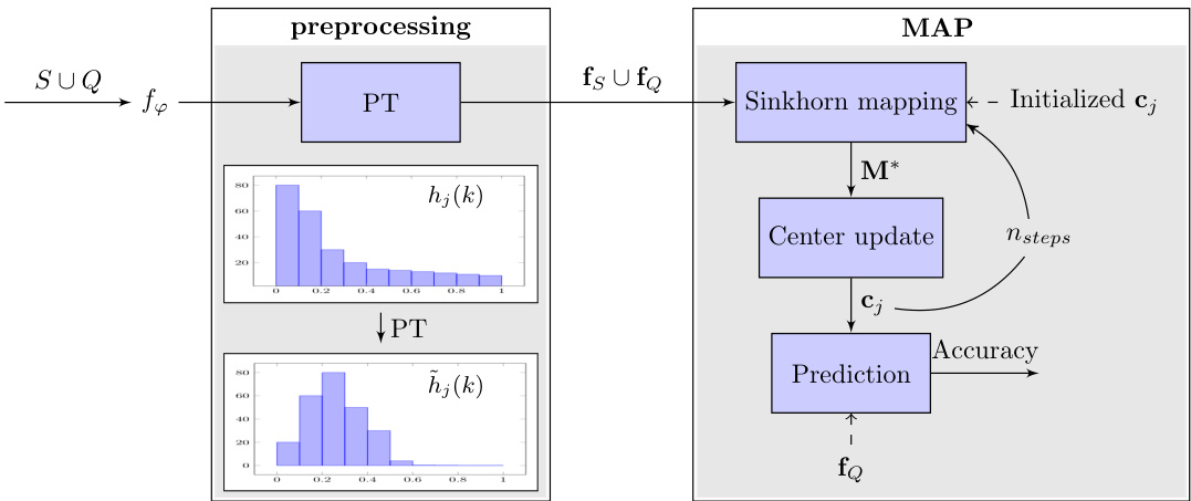
Figure 1: Illustration of the proposed method. First we extract feature vectors of all the inputs in $\mathbf{D}{n o v e l}$ and preprocess them to obtain $\mathbf{f}{S}\cup\mathbf{f}{Q}$ . Note that the Power transform (PT) has the effect of mapping a skewed feature distribution into a gaussian-like distribution ( $h{j}(k)$ denotes the histogram of feature $k$ in class $j$ ). In MAP, we perform Sinkhorn mapping with class center $\mathbf{c}{j}$ initialized on fS to obtain the class allocation matrix $\mathbf{M}^{*}$ for $\mathbf{f}{Q}$ , and we update the class centers for the next iteration. After $\boldsymbol{n_{s t e p s}}$ we evaluate the accuracy on $\mathbf{f}_{Q}$ .
图 1: 所提出方法的示意图。首先,我们提取 $\mathbf{D}{n o v e l}$ 中所有输入的特征向量,并对它们进行预处理以获得 $\mathbf{f}{S}\cup\mathbf{f}{Q}$。注意,幂变换 (PT) 的效果是将偏斜的特征分布映射为类似高斯分布($h{j}(k)$ 表示类 $j$ 中特征 $k$ 的直方图)。在 MAP 中,我们在 fS 上初始化的类中心 $\mathbf{c}{j}$ 上执行 Sinkhorn 映射,以获得 $\mathbf{f}{Q}$ 的类分配矩阵 $\mathbf{M}^{*}$,并为下一次迭代更新类中心。在 $\boldsymbol{n_{s t e p s}}$ 之后,我们评估 $\mathbf{f}_{Q}$ 上的准确率。
2 Related work
2 相关工作
A large volume of works in few-shot classification is based on meta learning [30] methods, where the training data is transformed into few-shot learning episodes to better fit in the context of few examples. In this branch, optimization based methods [30, 8, 23] train a well-initialized optimizer so that it quickly adapts to unseen classes with a few epochs of training. Other works [41, 4] utilize data augmentation techniques to artificially increase the size of the training datasets.
少样本分类领域的大量工作基于元学习 (meta learning) [30] 方法,其中训练数据被转换为少样本学习任务,以更好地适应少量样本的场景。在这一分支中,基于优化的方法 [30, 8, 23] 训练一个良好初始化的优化器,使其能够通过少量训练周期快速适应未见过的类别。其他工作 [41, 4] 则利用数据增强技术,人为增加训练数据集的规模。
In the past few years, there have been a growing interest in transfer-based methods. The main idea consists in training feature extractors able to efficiently segregate novel classes it never saw before. For example, in [3] the authors train the backbone with a distance-based classifier [22] that takes into account the inter-class distance. In [21], the authors utilize self-supervised learning techniques [2] to co-train an extra rotation classifier for the output features, improving the accuracy in few-shot settings. Many approaches are built on top of a feature extractor. For instance, in [38] the authors implement a nearest class mean classifier to associate an input with a class whose centroid is the closest in terms of the $\ell_{2}$ distance. In [18] an iterative approach is used to adjust the class centers. In [13] the authors build a graph neural neural network to gather the feature information from similar samples. Transferbased techniques typically reach the best performance on standardized benchmarks.
过去几年,基于迁移的方法引起了越来越多的关注。其主要思想是训练特征提取器,使其能够有效分离从未见过的新类别。例如,在 [3] 中,作者使用基于距离的分类器 [22] 训练骨干网络,该分类器考虑了类间距离。在 [21] 中,作者利用自监督学习技术 [2] 共同训练一个额外的旋转分类器来处理输出特征,从而提高了少样本设置中的准确性。许多方法都是基于特征提取器构建的。例如,在 [38] 中,作者实现了一个最近类均值分类器,将输入与在 $\ell_{2}$ 距离上最接近的类中心相关联。在 [18] 中,使用迭代方法来调整类中心。在 [13] 中,作者构建了一个图神经网络,以从相似样本中收集特征信息。基于迁移的技术通常在标准化基准测试中达到最佳性能。
Although many works involve feature extraction, few have explored the features in terms of their distribution [11]. Often, assumptions are made that the features in a class align to a certain distribution, even though these assumptions are rarely experimentally discussed. In our work, we analyze the impact of the features distributions and how they can be transformed for better processing and accuracy. We also introduce a new algorithm to improve the quality of the association between input features and corresponding classes in typical few-shot settings.
虽然许多工作涉及特征提取,但很少有研究从特征分布的角度进行探讨 [11]。通常,人们会假设某一类别的特征符合某种分布,尽管这些假设很少通过实验进行讨论。在我们的工作中,我们分析了特征分布的影响,以及如何通过转换特征来提高处理效率和准确性。我们还引入了一种新算法,以在典型的少样本设置中改善输入特征与对应类别之间的关联质量。
Contributions. Let us highlight the main contributions of this work. (1) We propose to preprocess the raw extracted features in order to make them more aligned with Gaussian assumptions. Namely we introduce transforms of the features so that they become less skewed. (2) We use a wasser stein-based method to better align the distribution of features with that of the considered classes. (3) We show that the proposed method can bring large increase in accuracy with a variety of feature extractors and datasets, leading to state-of-the-art results in the considered benchmarks.
贡献。让我们重点介绍这项工作的主要贡献。(1) 我们提出对原始提取的特征进行预处理,以使它们更符合高斯假设。具体来说,我们引入了特征的变换,以减少它们的偏斜。(2) 我们使用基于Wasserstein距离的方法,以更好地将特征的分布与所考虑的类别的分布对齐。(3) 我们展示了所提出的方法可以在多种特征提取器和数据集上带来显著的准确率提升,从而在所考虑的基准测试中取得了最先进的结果。
3 Methodology
3 方法论
In this section we introduce the problem settings. We discuss the training of the feature extractors, the preprocessing steps that we apply on the trained features and the final classification algorithm. A summary of our proposed method is depicted in Figure 1.
在本节中,我们介绍了问题设置。我们讨论了特征提取器的训练、对训练特征进行的预处理步骤以及最终的分类算法。我们提出的方法总结如图1所示。
3.1 Problem statement
3.1 问题陈述
We consider a typical few-shot learning problem. We are given a base dataset $\mathbf{D}{b a s e}$ and a novel dataset $\mathbf{D}{n o v e l}$ such that $\mathbf{D}{b a s e}\cap\mathbf{D}{n o v e l}=\emptyset$ . $\mathbf{D}{b a s e}$ contains a large number of labelled examples from $K$ different classes. $\mathbf{D}{n o v e l}$ , also referred to as a task in other works, contains a small number of labelled examples (support set $S$ ), along with some unlabelled ones (query set $Q$ ), all from $w$ new classes. Our goal is to predict the class of the unlabelled examples in the query set. The following parameters are of particular importance to define such a few-shot problem: the number of classes in the novel dataset $w$ (called $w$ -way), the number of labelled samples per class $s$ (called $s$ -shot) and the number of unlabelled samples per class $q$ . So the novel dataset contains a total of $w(s+q)$ samples, $w s$ of them being labelled, and $w q$ of them being those to classify. In the case of inductive few-shot, the prediction is performed independently on each one of the $w q$ samples. In the case of trans duct ive few-shot [20, 18], the prediction is performed considering all $w q$ samples together. In the latter case, most works exploit the information that there are exactly $q$ samples in each class. We discuss this point in the experiments.
我们考虑一个典型的少样本学习问题。给定一个基础数据集 $\mathbf{D}{base}$ 和一个新数据集 $\mathbf{D}{novel}$,且 $\mathbf{D}{base}\cap\mathbf{D}{novel}=\emptyset$。$\mathbf{D}{base}$ 包含来自 $K$ 个不同类别的大量标注样本。$\mathbf{D}{novel}$(在其他工作中也称为任务)包含少量标注样本(支持集 $S$)以及一些未标注样本(查询集 $Q$),所有这些样本都来自 $w$ 个新类别。我们的目标是预测查询集中未标注样本的类别。以下参数对于定义这样的少样本问题尤为重要:新数据集中的类别数 $w$(称为 $w$-way),每个类别的标注样本数 $s$(称为 $s$-shot),以及每个类别的未标注样本数 $q$。因此,新数据集总共包含 $w(s+q)$ 个样本,其中 $ws$ 个是标注的,$wq$ 个是需要分类的。在归纳少样本的情况下,预测是独立地对每个 $wq$ 样本进行的。在转导少样本的情况下 [20, 18],预测是考虑所有 $wq$ 样本一起进行的。在后一种情况下,大多数工作利用了每个类别中恰好有 $q$ 个样本的信息。我们在实验中讨论了这一点。
3.2 Feature extraction
3.2 特征提取
The first step is to train a neural network backbone model using only the base dataset. In this work we consider multiple backbones, with various training procedures. Once the considered backbone is trained, we obtain robust embeddings that should generalize well to novel classes. We denote by $f_{\varphi}$ the backbone function, obtained by extracting the output of the penultimate layer from the considered architecture, with $\varphi$ being the trained architecture parameters. Note that importantly, in all backbone architectures used in the experiments of this work, the penultimate layers are obtained by applying a ReLU function, so that all feature components coming out of $f_{\varphi}$ are non negative.
第一步是仅使用基础数据集训练一个神经网络骨干模型。在本工作中,我们考虑了多个骨干模型,并采用了不同的训练方法。一旦所考虑的骨干模型训练完成,我们就能获得鲁棒的嵌入,这些嵌入应该能够很好地泛化到新类别。我们用 $f_{\varphi}$ 表示骨干函数,该函数通过从所考虑的架构中提取倒数第二层的输出获得,其中 $\varphi$ 是训练好的架构参数。需要注意的是,在本工作的所有实验中使用的骨干架构中,倒数第二层是通过应用 ReLU 函数获得的,因此从 $f_{\varphi}$ 输出的所有特征分量都是非负的。
3.3 Feature preprocessing
3.3 特征预处理
As mentioned in Section 2, many works hypothesize, explicitly or not, that the features from the same class are aligned with a specific distribution (often Gaussianlike). But this aspect is rarely experimentally verified. In fact, it is very likely that features obtained using the backbone architecture are not Gaussian. Indeed, usually the features are obtained after applying a relu function, and exhibit a positive distribution mostly concentrated around 0 (see details in the next section).
如第2节所述,许多工作明确或隐含地假设来自同一类别的特征与特定分布(通常是类高斯分布)对齐。但这一方面很少经过实验验证。事实上,使用骨干架构获得的特征很可能不是高斯分布。实际上,通常特征是在应用ReLU函数后获得的,并且呈现出主要集中在0附近的正分布(详见下一节)。
Multiple works in the domain [38, 18] discuss the different statistical methods (e.g. normalization) to better fit the features into a model. Although these methods may have provable assets for some distributions, they could worsen the process if applied to an unexpected input distribution. This is why we propose to preprocess the obtained feature vectors so that they better align with typical distribution assumptions in the field. Namely, we use a power transform as follows.
该领域中的多项研究 [38, 18] 讨论了不同的统计方法(例如归一化),以更好地将特征拟合到模型中。尽管这些方法可能对某些分布具有可证明的优势,但如果应用于意外的输入分布,可能会使过程恶化。这就是为什么我们建议对获得的特征向量进行预处理,以便它们更好地与该领域的典型分布假设对齐。具体而言,我们使用如下的幂变换。
Power transform (PT). Denote $\textbf{v}=\mathbf{\nabla}f_{\varphi}(\mathbf{x})\in\mathbf{\sigma}$ $(\mathbb{R}^{+})^{d},\mathbf{x}\in\mathbf{D}{n o v e l}$ as the obtained features on $\mathbf{D}{n o v e l}$ We hereby perform a power transformation method, which is similar to Tukey’s Transformation Ladder [32], on the features. We then follow a unit variance projection, the formula is given by:
幂变换 (PT)。设 $\textbf{v}=\mathbf{\nabla}f_{\varphi}(\mathbf{x})\in\mathbf{\sigma}$ $(\mathbb{R}^{+})^{d},\mathbf{x}\in\mathbf{D}{n o v e l}$ 为在 $\mathbf{D}{n o v e l}$ 上获得的特征。我们在此对特征进行一种类似于 Tukey 变换阶梯 [32] 的幂变换方法。随后,我们进行单位方差投影,公式如下:

where $\epsilon=1e{-6}$ is used to make sure that ${\mathbf{v}}\boldsymbol{+}\epsilon$ is strictly positive and $\beta$ is a hyper-parameter. The rationales of the preprocessing above are: (1) Power transforms have the functionality of reducing the skew of a distribution, adjusted by $\beta$ , (2) Unit variance projection scales the features to the same area so that large variance features do not predominate the others. This preprocessing step is often able to map data from any distribution to a close-to-Gaussian distribution. We will analyse this ability and the effect of power transform in more details in Section 4.
其中 $\epsilon=1e{-6}$ 用于确保 ${\mathbf{v}}\boldsymbol{+}\epsilon$ 严格为正,$\beta$ 是一个超参数。上述预处理的原理是:(1) 幂变换具有减少分布偏斜的功能,通过 $\beta$ 进行调整,(2) 单位方差投影将特征缩放到相同的区域,使得大方差特征不会主导其他特征。此预处理步骤通常能够将任何分布的数据映射到接近高斯分布。我们将在第4节中更详细地分析这种能力以及幂变换的效果。
Note that $\beta=1$ leads to almost no effect. More generally, the skew of the obtained distribution changes when $\beta$ varies. For instance, if a raw distribution is rightskewed, decreasing $\beta$ phases out the right skew, and phases into a left-skewed distribution when $\beta$ becomes negative. After experiments, we found that $\beta=0.5$ gives the most consistent results for our considered experiments. More details based on our considered experiments are available in Section 4.
注意到当 $\beta=1$ 时,几乎没有任何效果。更一般地,当 $\beta$ 变化时,所获得分布的偏斜度也会发生变化。例如,如果原始分布是右偏的,减小 $\beta$ 会逐渐消除右偏,并在 $\beta$ 变为负值时逐渐转变为左偏分布。经过实验,我们发现 $\beta=0.5$ 在我们所考虑的实验中给出了最一致的结果。更多基于我们实验的细节见第4节。
This first step of feature preprocessing can be performed in both inductive and trans duct ive settings.
特征预处理的第一步可以在归纳和传导两种设置下进行。
3.4 MAP
3.4 MAP
Let us assume that the pre processed feature distribution for each class is Gaussian or Gaussian-like. As such, a well-positioned class center is crucial to a good prediction. In this section we discuss how to best estimate the class centers when the number of samples is very limited and classes are only partially labelled. In more details, we propose an Expectation–Maximization [7]- like algorithm that will iterative ly find the Maximum A Posteriori (MAP) estimates of the class centers.
假设每个类别的预处理特征分布是高斯或类高斯的。因此,一个良好定位的类别中心对于良好的预测至关重要。在本节中,我们讨论了在样本数量非常有限且类别仅部分标记的情况下,如何最好地估计类别中心。更详细地说,我们提出了一种类似于期望最大化 (Expectation–Maximization) [7] 的算法,该算法将迭代地找到类别中心的最大后验 (Maximum A Posteriori, MAP) 估计。
We firstly show that estimating these centers through MAP is similar to the minimization of Wasser stein distance. Then, an iterative procedure based on a Wasser stein distance estimation, using the sinkhorn algorithm [5, 33, 14], is designed to estimate the optimal transport from the initial distribution of the feature vectors to one that would correspond to the draw of samples from Gaussian distributions.
我们首先展示了通过最大后验概率 (MAP) 估计这些中心与最小化 Wasserstein 距离的相似性。然后,设计了一种基于 Wasserstein 距离估计的迭代过程,使用 sinkhorn 算法 [5, 33, 14],以估计从特征向量的初始分布到与从高斯分布中抽取样本相对应的分布的最优传输。
Note that in this step we consider what is called the “trans duct ive” setting in many other few shot learning works [20, 18, 19, 13, 17, 9, 16, 10, 39], where we exploit unlabelled samples during the procedure as well as priors about their relative proportions.
请注意,在这一步中,我们考虑了许多其他少样本学习工作中所谓的“转导式”设置 [20, 18, 19, 13, 17, 9, 16, 10, 39],其中我们在过程中利用了未标记的样本以及它们相对比例的先验信息。
In the following, we denote by $\mathbf{f}{S}$ the set of feature vectors corresponding to labelled inputs and by fQ the set of feature vectors corresponding to unlabelled inputs. For a feature vector $\mathbf{f}\in\mathbf{f}{S}\cup\mathbf{f}{Q}$ , we denote by $\ell(\mathbf{f})$ the corresponding label. We use $0<i\leq w q$ to denote the index of an unlabelled sample, so that $\mathbf{f}{Q}=(\mathbf{f}{i}){i}$ , and we denote $\mathbf{c}_{j},0<j\leq w$ the estimated center for feature vectors corresponding to class $j$ .
在下文中,我们用 $\mathbf{f}{S}$ 表示标记输入对应的特征向量集合,用 $\mathbf{f}{Q}$ 表示未标记输入对应的特征向量集合。对于特征向量 $\mathbf{f}\in\mathbf{f}{S}\cup\mathbf{f}{Q}$,我们用 $\ell(\mathbf{f})$ 表示其对应的标签。我们使用 $0<i\leq w q$ 表示未标记样本的索引,因此 $\mathbf{f}{Q}=(\mathbf{f}{i}){i}$,并用 $\mathbf{c}{j},0<j\leq w$ 表示类别 $j$ 对应的特征向量的估计中心。
Our algorithm consists in several steps in which we estimate class centers from a soft allocation matrix $\mathbf{M}^{*}$ , then we update the allocation matrix based on the newly found class centers and iterate the process. In the following paragraphs, we detail these steps.
我们的算法由几个步骤组成,在这些步骤中,我们从软分配矩阵 $\mathbf{M}^{*}$ 中估计类中心,然后根据新找到的类中心更新分配矩阵,并迭代该过程。在接下来的段落中,我们将详细描述这些步骤。
Sinkhorn mapping. Considering using MAP estimation for the class centers, and assuming a Gaussian distribution for each class, we typically aim at solving:
Sinkhorn映射。考虑使用最大后验概率估计(MAP estimation)来估计类别中心,并假设每个类别服从高斯分布,我们通常旨在解决:

where $\mathit{c}$ represents the set of admissible labelling sets. Let us point out that the last term corresponds exactly to the Wasser stein distance used in the Optimal Transport problem formulation [5].
其中 $\mathit{c}$ 表示可接受的标签集集合。我们指出,最后一项正好对应于最优传输问题公式中使用的 Wasserstein 距离 [5]。
Therefore, in this step we find the class mapping matrix that minimizes the Wasser stein distance. Inspired by the Sinkhorn algorithm [35, 5], we define the mapping matrix $\mathbf{M}^{*}$ as follows:
因此,在这一步中,我们寻找最小化 Wasserstein 距离的类别映射矩阵。受 Sinkhorn 算法 [35, 5] 的启发,我们将映射矩阵 $\mathbf{M}^{*}$ 定义如下:

where $\mathbb{U}(\mathbf{p},\mathbf{q})\in\mathbb{R}_{+}^{w q\times w}$ is a set of positive matrices for which the rows sum to $\mathbf{p}$ and the columns sum to $\mathbf{q}$ . Formally, $\mathbb{U}(\mathbf{p},\mathbf{q})$ can be written as:
其中 $\mathbb{U}(\mathbf{p},\mathbf{q})\in\mathbb{R}_{+}^{w q\times w}$ 是一组正矩阵,其行和为 $\mathbf{p}$,列和为 $\mathbf{q}$。形式上,$\mathbb{U}(\mathbf{p},\mathbf{q})$ 可以写成:

$\mathbf{p}$ denotes the distribution of the amount that each unlabelled example uses for class allocation, and $\mathbf{q}$ denotes the distribution of the amount of unlabelled examples allocated to each class. Therefore, $\mathbb{U}(\mathbf{p},\mathbf{q})$ contains all the possible ways of allocating examples to classes. The cost function $\mathbf{L}\in\mathbb{R}^{w q\times w}$ in Equation (3) consists of the euclidean distances between unlabelled examples and class centers, hence $\mathbf{L}_{i j}$ denotes the euclidean distance between example $i$ and class center $j$ . Here we assume a soft class mapping, meaning that each example can be “sliced” into different classes.
$\mathbf{p}$ 表示每个未标记样本用于类别分配的量的分布,$\mathbf{q}$ 表示分配给每个类别的未标记样本的量的分布。因此,$\mathbb{U}(\mathbf{p},\mathbf{q})$ 包含了所有将样本分配到类别的可能方式。公式 (3) 中的成本函数 $\mathbf{L}\in\mathbb{R}^{w q\times w}$ 由未标记样本与类别中心之间的欧几里得距离组成,因此 $\mathbf{L}_{i j}$ 表示样本 $i$ 与类别中心 $j$ 之间的欧几里得距离。这里我们假设一个软类别映射,意味着每个样本可以被“切片”到不同的类别中。
The second term on the right of Equation (3) denotes the entropy of M: $\begin{array}{r}{H(\mathbf{M})=-\sum_{i j}\mathbf{M}{i j}\log\mathbf{M}{i j}}\end{array}$ , regu- larized by a hyper-parameter $\lambda$ . Increasing $\lambda$ would force the entropy to become smaller, so that the mapping is less homogeneous. This term also makes the objective function strictly convex [5, 29] and thus a practical and effective computation. From lemma 2 in [5], the result of this Sinkhorn mapping has the typical form $\mathbf{M}^{*}=\mathrm{diag}(\mathbf{u})\cdot\exp(-\mathbf{L}/\lambda)\cdot\mathrm{diag}(\mathbf{v})$ .
方程 (3) 右边的第二项表示 M 的熵:$\begin{array}{r}{H(\mathbf{M})=-\sum_{i j}\mathbf{M}{i j}\log\mathbf{M}{i j}}\end{array}$,通过超参数 $\lambda$ 进行正则化。增加 $\lambda$ 会使熵变小,从而使映射更加不均匀。这一项还使目标函数严格凸 [5, 29],从而实现了实用且有效的计算。根据 [5] 中的引理 2,这种 Sinkhorn 映射的结果具有典型形式 $\mathbf{M}^{*}=\mathrm{diag}(\mathbf{u})\cdot\exp(-\mathbf{L}/\lambda)\cdot\mathrm{diag}(\mathbf{v})$。
Iterative center estimation. In this step, our aim is to estimate class centers. As shown in Algorithm 1, we initialize $\mathbf{c}{j}$ as the average of labelled samples belonging to class $j$ . Then $\mathbf{c}{j}$ is iterative ly re-estimated. At each iteration, we compute a mapping matrix M $^*$ on the unlabelled examples using the sinkhorn mapping. Along with labelled examples, we re-estimate $\mathbf{c}{j}$ (temporarily denoted $\pmb{\mu}{j}$ ) by weighted-averaging the features with their allocated portions for class $j$ :
迭代中心估计。在这一步中,我们的目标是估计类别中心。如算法 1 所示,我们将 $\mathbf{c}{j}$ 初始化为属于类别 $j$ 的标记样本的平均值。然后,$\mathbf{c}{j}$ 被迭代地重新估计。在每次迭代中,我们使用 sinkhorn 映射在未标记样本上计算映射矩阵 M $^*$。结合标记样本,我们通过加权平均特征及其分配给类别 $j$ 的部分来重新估计 $\mathbf{c}{j}$(暂时表示为 $\pmb{\mu}{j}$):
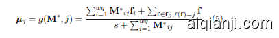
This formula corresponds to the minimization of Equation (3). Note that labelled examples do not participate in the mapping process. Since their labels are known, we instead set allocations for their belonging classes to be 1 and to the others to be $0$ . Therefore, labelled examples have the largest possible weight when re-estimating the class centers.
该公式对应于方程 (3) 的最小化。需要注意的是,已标注的样本不参与映射过程。由于它们的标签已知,我们将其所属类别的分配设置为 1,其他类别设置为 $0$。因此,在重新估计类别中心时,已标注的样本具有最大的权重。
Proportioned center update. In order to avoid taking risky harsh decisions in early iterations of the algorithm, we propose to proportionate the update of class centers using an inertia parameter. In more details, we update the center with a learning rate $0<$ $\alpha\leq1$ . When $\alpha$ is close to $0$ , the update becomes very slow, whereas $\alpha=1$ corresponds to directly allocating the newly found class centers:
比例中心更新。为了避免在算法的早期迭代中做出风险较大的激进决策,我们提出使用惯性参数来按比例更新类别中心。具体来说,我们以学习率 $0<$ $\alpha\leq1$ 更新中心。当 $\alpha$ 接近 $0$ 时,更新变得非常缓慢,而 $\alpha=1$ 则对应于直接分配新找到的类别中心:

Final decision. After a fixed number of steps nsteps, the rows of $\mathbf{M}^{*}$ are interpreted as probabilities to belong to each class. The maximal value corresponds to the decision of the algorithm.
最终决策。经过固定步骤数 nsteps 后,$\mathbf{M}^{*}$ 的行被解释为属于每个类别的概率。最大值对应算法的决策。
A summary of our proposed algorithm is presented in Algorithm 1. In Table 1 we summarize the main parameters and hyper parameters of the considered problem and proposed solution. The code is available at XXX.
我们提出的算法总结见算法 1。在表 1 中,我们总结了所考虑问题和提出解决方案的主要参数和超参数。代码可在 XXX 获取。
4 Experiments
4 实验
4.1 Datasets
4.1 数据集
We evaluate the performance of the proposed method using standardized few-shot classification datasets: mini Image Net [36], tiered Image Net [24], CUB [37] and
我们使用标准化的少样本分类数据集评估所提出方法的性能:mini ImageNet [36]、tiered ImageNet [24]、CUB [37] 和
算法 1: 提出的算法
参数 :w, s, q, 入, Q, Nsteps
f
重复 nsteps 次: Lij = |f - cll², V, j M* = Sinkhorn(L, p = lwq, q = qlw, ^)
CIFAR-FS [1]. The mini Image Net dataset contains 100 classes randomly chosen from ILSVRC- 2012 [25] and 600 images of size $84\times84$ pixels per class. It is split into 64 base classes, 16 validation classes and 20 novel classes. The tiered Image Net dataset is another subset of ImageNet, it consists of 34 high-level categories with 608 classes in total. These categories are split into 20 meta-training super classes, 6 meta-validation superclasses and 8 meta-test super classes, which corresponds to 351 base classes, 97 validation classes and 160 novel classes respectively. The CUB dataset contains 200 classes and has 11,788 images of size $84\times84$ pixels in total. Following [13], it is split into 100 base classes, 50 validation classes and 50 novel classes. The CIFARFS dataset has 100 classes, each class contains 600 images of size $32\times32$ pixels. The splits of this dataset are the same as those in mini Image Net.
CIFAR-FS [1]。mini Image Net 数据集包含从 ILSVRC-2012 [25] 中随机选择的 100 个类别,每个类别有 600 张大小为 $84\times84$ 像素的图像。它被分为 64 个基础类别、16 个验证类别和 20 个新类别。tiered Image Net 数据集是 ImageNet 的另一个子集,它包含 34 个高级类别,总共有 608 个类别。这些类别被分为 20 个元训练超类、6 个元验证超类和 8 个元测试超类,分别对应 351 个基础类别、97 个验证类别和 160 个新类别。CUB 数据集包含 200 个类别,总共有 11,788 张大小为 $84\times84$ 像素的图像。根据 [13],它被分为 100 个基础类别、50 个验证类别和 50 个新类别。CIFARFS 数据集有 100 个类别,每个类别包含 600 张大小为 $32\times32$ 像素的图像。该数据集的划分与 mini Image Net 相同。
4.2 Implementation details
4.2 实现细节
In order to stress the genericity of our proposed method with regards to the chosen backbone architecture and training strategy, we perform experiments using WRN [40], ResNet18 and ResNet12 [12], along with some other pretrained backbones (e.g. DenseNet [15]). For each dataset we train the feature extractor with base classes, tune the hyper parameters with validation classes and test the performance using novel classes. Therefore, for each test run, $w$ classes are drawn uniformly at random among novel classes. Among these $w$ classes, $s$ labelled examples and $q$ unlabelled examples per class are uniformly drawn at random to form $\mathbf{D}_{n o v e l}$ . The WRN and ResNet are trained following [21]. In the inductive setting, we use our proposed Power Transform followed by a basic Nearest Class Mean (NCM) classifier. In the transductive setting, the MAP or an alternative is applied after PT. In order to better segregate between feature vectors of corresponding classes for each task, we implement the “trans-mean-sub” [18] before MAP where we separately subtract inputs by the means of labelled and unlabelled examples, followed by a unit hyper sphere projection. All our experiments are performed using $w=5,q=15$ , $s=1$ or 5. We run 10,000 random draws to obtain mean accuracy score and indicate confidence scores (95%) when relevant. The tuned hyperparameters for mini Image Net are $\beta=0.5,\lambda=10,\alpha=0.4$ and $n_{s t e p s}=30$ for $s=1$ ; $\beta=0.5,\lambda=10,\alpha=0.2$ and $n_{s t e p s}=20$ for $s=5$ . Hyper parameters for other datasets are detailed in the experiments below.
为了强调我们提出的方法在选择骨干架构和训练策略方面的通用性,我们使用 WRN [40]、ResNet18 和 ResNet12 [12] 以及其他一些预训练骨干(例如 DenseNet [15])进行实验。对于每个数据集,我们使用基础类训练特征提取器,使用验证类调整超参数,并使用新类测试性能。因此,对于每次测试运行,从新类中均匀随机抽取 $w$ 个类。在这些 $w$ 个类中,每个类均匀随机抽取 $s$ 个标记样本和 $q$ 个未标记样本,形成 $\mathbf{D}_{n o v e l}$。WRN 和 ResNet 的训练遵循 [21]。在归纳设置中,我们使用提出的 Power Transform,然后使用基本的最近类均值 (NCM) 分类器。在转导设置中,PT 后应用 MAP 或替代方法。为了更好地分离每个任务中对应类的特征向量,我们在 MAP 之前实现“trans-mean-sub” [18],其中我们分别减去标记和未标记样本的均值,然后进行单位超球投影。所有实验均使用 $w=5,q=15$,$s=1$ 或 5 进行。我们运行 10,000 次随机抽取以获得平均准确率分数,并在相关时指示置信分数 (95%)。mini Image Net 的超参数调整为 $s=1$ 时 $\beta=0.5,\lambda=10,\alpha=0.4$ 和 $n_{s t e p s}=30$;$s=5$ 时 $\beta=0.5,\lambda=10,\alpha=0.2$ 和 $n_{s t e p s}=20$。其他数据集的超参数在以下实验中详细说明。
4.3 Comparison with state-of-the-art methods
4.3 与最先进方法的比较
In the first experiment, we conduct our proposed method on different benchmarks and compare the performance with other state-of-the-art solutions. The results are presented in Table 2, we observe that our method with WRN as backbone reaches the state-ofthe-art performance for most cases in both inductive and trans duct ive settings on all the benchmarks. In Table 3 we also implement our proposed method on tiered Image Net based on a pre-trained Dense Net 121 backbone following the procedure described in [38]. From these experiments we conclude that the proposed method can bring an increase of accuracy with a variety of backbones and datasets, leading to competitive performance. In terms of execution time, we measured an average of $0.002s$ per run.
在第一个实验中,我们在不同的基准上进行了我们提出的方法,并将其性能与其他最先进的解决方案进行了比较。结果如表 2 所示,我们观察到,使用 WRN 作为骨干网络的方法在大多数情况下,在所有基准的归纳和传导设置中均达到了最先进的性能。在表 3 中,我们还基于预训练的 DenseNet 121 骨干网络,按照 [38] 中描述的程序,在分层 ImageNet 上实现了我们提出的方法。通过这些实验,我们得出结论:所提出的方法可以在多种骨干网络和数据集上提高准确性,从而带来具有竞争力的性能。在执行时间方面,我们测得每次运行的平均时间为 $0.002s$。
Performance on cross-domain settings. We also test our method in a cross-domain setting, where the backbone is trained with the base classes in miniImageNet but tested with the novel classes in CUB dataset. As shown in Table 4, the proposed method gives the best accuracy both in the case of 1-shot and 5-shot.
跨域设置下的性能。我们还在跨域设置中测试了我们的方法,其中骨干网络在miniImageNet的基础类上进行训练,但在CUB数据集的新类上进行测试。如表4所示,所提出的方法在1-shot和5-shot情况下均提供了最佳准确率。
4.4 Other experiments
4.4 其他实验
Ablation study. To prove the interest of the ingredients on the proposed method in order to reach top performance, we report in Tables 5 and 6 the results of ablation studies. In Table 5, we first investigate the impact of changing the backbone architecture. Together with previous experiments, we observe that the proposed method consistently achieves the best results for any fixed backbone architecture. We also report performance in the case of inductive few-shot using a simple Nearest-Class Mean (NCM) classifier instead of the iterative MAP procedure described in Section 3. We perform another experiment where we replace the MAP algorithm with a standard K-Means where centroids are initialized with the available labelled samples for each class. We can observe significant drops in accuracy, emphasizing the interest of the proposed MAP procedure to better estimate the class centers.
消融研究。为了证明所提出方法中各成分对达到最佳性能的重要性,我们在表 5 和表 6 中报告了消融研究的结果。在表 5 中,我们首先研究了改变骨干架构的影响。结合之前的实验,我们观察到所提出的方法在任何固定的骨干架构下都能始终取得最佳结果。我们还报告了在使用简单的最近类均值 (Nearest-Class Mean, NCM) 分类器代替第 3节中描述的迭代 MAP 过程时的归纳少样本性能。我们进行了另一个实验,将 MAP 算法替换为标准 K-Means,其中每个类的中心用可用的标记样本初始化。我们可以观察到准确率的显著下降,这强调了所提出的 MAP 过程在更好地估计类中心方面的重要性。
In Table 6 we show the impact of PT in the trans duct ive setting, where we can see about 6% gain for 1-shot and
在表 6 中,我们展示了 PT 在传导设置中的影响,可以看到在 1-shot 情况下有约 6% 的提升。
Table 1: Important parameters and hyper parameters.
表 1: 重要参数和超参数
| Notation | Value | Description |
|---|---|---|
| Novel dataset parameters | ||
| 通常为 5 | 类别数量 | |
| S | 通常为 1 或 5 | 每个类别的标记输入数量 |
| q | 通常为 15 | 每个类别的未标记输入数量 |
| Proposed method hyperparameters | ||
| Notation | Range | Description |
| β | {-2, -1, -0.5, 0, 0.5, 1, 2} | 调整分布偏斜的系数 |
| 入 | 入 ∈ R+ | Sinkhorn 映射的正则化系数 |
| I > ∞ > 0 | 类别中心更新的学习率 |
$4%$ gain for 5-shot in terms of accuracy.
在准确率方面,5-shot 提升了 4%。
Effect of Power Transform. To visualize the effect of PT on the feature distributions, we depict in Figure 2 the distributions of an arbitrarily selected feature for 5 randomly selected novel classes of mini Image Net when using WRN, before and after applying PT. We observe quite clearly how PT is able to reshape the feature distributions to close-to-gaussian distributions. We observed similar behaviors with other datasets as well.
功率变换的效果。为了可视化功率变换(PT)对特征分布的影响,我们在图2中展示了使用WRN时,mini Image Net数据集中随机选择的5个新类别中任意一个特征在应用PT前后的分布情况。我们可以清楚地观察到PT如何将特征分布重塑为接近高斯分布。我们在其他数据集上也观察到了类似的行为。

Figure 2: Distributions of an arbitrarily chosen feature for 5 novel classes before $(a)$ and after (b) PT.
图 2: 在 PT 之前 $(a)$ 和之后 (b) 5 个新类别的任意选定特征的分布。
Influence of the number of unlabelled samples. Small values of $q$ lead to settings that are closer to the inductive case. In order to better understand the gain in accuracy due to having access to more unlabelled samples, we depict in Figure 4 the evolution of accuracy as a function of $q$ , when $w=5$ is fixed. Interestingly, the accuracy quickly reaches a close-to-asymptotic al plateau, emphasizing the ability of the method to soon exploit available information in the task.
未标记样本数量的影响。较小的 $q$ 值会导致更接近归纳情况的设置。为了更好地理解由于访问更多未标记样本而带来的准确性提升,我们在图 4 中描绘了当 $w=5$ 固定时,准确性随 $q$ 变化的演变。有趣的是,准确性迅速达到接近渐近的平台期,强调了该方法能够迅速利用任务中可用信息的能力。
Impact of class imbalance. In all previous transductive experiments, we assumed a balanced number of unlabelled samples per class. We now consider the case of 2 classes, where we vary the number of unlabelled examples $q1$ of class 1 with respect to that of class 2 $(100-q1)$ . In Figure 3 we depict: 1) the performance of the inductive version of our method (PT-NCM), which is independent of $q1$ , 2) the performance of the proposed trans duct ive method when the vector $\mathbf{q}$ is appropriately defined (knowing the proportion of elements in class 1 vs. class 2), and 3) a mixed case where we expect at least 30 elements in both classes but do not know exactly how many ( $\mathbf{q}=[30,30]$ ). Interestingly, we observe that the trans duct ive setting still outperforms the inductive ones even when the proportion of elements in both classes is only approximately known.
类别不平衡的影响。在之前的所有转导实验中,我们假设每个类别的未标记样本数量是平衡的。现在我们考虑两个类别的情况,其中我们改变类别1的未标记样本数量 $q1$ 相对于类别2的未标记样本数量 $(100-q1)$ 。在图3中,我们展示了:1)我们方法的归纳版本(PT-NCM)的性能,它与 $q1$ 无关;2)当向量 $\mathbf{q}$ 被正确定义时(知道类别1与类别2的元素比例),所提出的转导方法的性能;3)混合情况,我们期望两个类别中至少有30个元素,但不知道确切数量( $\mathbf{q}=[30,30]$ )。有趣的是,我们观察到,即使两个类别的元素比例只是大致已知,转导设置仍然优于归纳设置。

Figure 3: Accuracy of 2-ways classification on miniImagenet (1-shot) with unevenly distributed query data for each class in different settings, where the total number of query inputs remains constant (total: 100 elements). When $q_{1}=1$ , we obtain the most imbalanced case, whereas $q_{1}=50$ corresponds to a balanced case.
图 3: 在不同设置下,miniImagenet 数据集上 2 分类的准确率(1-shot),其中每个类别的查询数据分布不均匀,但查询输入的总数保持不变(总计:100 个元素)。当 $q_{1}=1$ 时,我们得到最不平衡的情况,而 $q_{1}=50$ 则对应平衡的情况。
Hyper parameter tuning. In the next experiment we tune $\beta,\lambda$ and $\alpha$ on the validation classes of each dataset, and then apply them to test our model on novel classes. We vary each hyper param ter in a certain range and observe the evolution of accuracy to choose the peak that corresponds to the highest prediction. For example, the evolving curve for $\beta,\lambda$ and $\alpha$ with mini Image Net are presented in Figure 4 (2) to (4). For comparison purposes, we also trace the corresponding curves on novel classes. We draw a dash line on the hyper parameter values where the accuracy on the validation classes peaks, meaning that this is the chosen value resulting in Table 2.
超参数调优。在接下来的实验中,我们调整 $\beta,\lambda$ 和 $\alpha$ 在每个数据集的验证类上,然后将它们应用于测试我们的模型在新类上的表现。我们在一定范围内改变每个超参数,并观察准确率的变化,以选择对应于最高预测的峰值。例如,$\beta,\lambda$ 和 $\alpha$ 在 mini Image Net 上的变化曲线如图 4 (2) 至 (4) 所示。为了比较,我们还在新类上追踪了相应的曲线。我们在验证类准确率达到峰值的超参数值处画了一条虚线,这意味着这是表 2 中所选的值。
Table 2: 1-shot and 5-shot accuracy of state-of-the-art methods in the literature, compared with the proposed solution. We present results using WRN as backbones for our proposed solutions.
表 2: 文献中最先进方法的 1-shot 和 5-shot 准确率,与提出的解决方案进行比较。我们展示了使用 WRN 作为我们提出的解决方案的骨干网络的结果。
| 设置 | 方法 | 骨干网络 | miniImageNet 1-shot | miniImageNet 5-shot |
|---|---|---|---|---|
| 归纳 | Baseline++ [3] | ResNet18 | 51.87 ± 0.77% | 75.68 ± 0.63% |
| 归纳 | MAML [8] | ResNet18 | 49.61 ± 0.92% | 65.72 ± 0.77% |
| 归纳 | ProtoNet [28] | WRN | 62.60 ± 0.20% | 79.97 ± 0.14% |
| 归纳 | Matching Networks [36] | WRN | 64.03 ± 0.20% | 76.32 ± 0.16% |
| 归纳 | SimpleShot [38] | DenseNet121 | 64.29 ± 0.20% | 81.50 ± 0.14% |
| 归纳 | S2M2_R [21] | WRN | 64.93 ± 0.18% | 83.18 ± 0.11% |
| 归纳 | PT+NCM (ours) | WRN | 65.35 ± 0.20% | 83.87 ± 0.13% |
| 转导 | BD-CSPN [19] | WRN | 70.31 ± 0.93% | 81.89 ± 0.60% |
| 转导 | Transfer+SGC [13] | WRN | 76.47 ± 0.23% | 85.23 ± 0.13% |
| 转导 | TAFSSL [18] | DenseNet121 | 77.06 ± 0.26% | 84.99 ± 0.14% |
| 转导 | DFMN-MCT [17] | ResNet12 | 78.55 ± 0.86% | 86.03 ± 0.42% |
| 转导 | PT+MAP (ours) | WRN | 82.92 ± 0.26% | 88.82 ± 0.13% |
| 设置 | 方法 | 骨干网络 | CUB 1-shot | CUB 5-shot |
| 归纳 | Baseline++ [3] | ResNet10 | 69.55 ± 0.89% | 85.17 ± 0.50% |
| 归纳 | MAML [8] | ResNet10 | 70.32 ± 0.99% | 80.93 ± 0.71% |
| 归纳 | ProtoNet [28] | ResNet18 | 72.99 ± 0.88% | 86.64 ± 0.51% |
| 归纳 | Matching Networks [36] | WRN | 73.49 ± 0.89% | 84.45 ± 0.58% |
| 归纳 | S2M2_R [21] | WRN | 80.68 ± 0.81% | 90.85 ± 0.44% |
| 归纳 | PT+NCM (ours) | WRN | 80.57 ± 0.20% | 91.15 ± 0.10% |
| 转导 | BD-CSPN [19] | WRN | 87.45% | 91.74% |
| 转导 | Transfer+SGC [13] | WRN | 88.35 ± 0.19% | 92.14 ± 0.10% |
| 转导 | PT+MAP (ours) | WRN | 91.55 ± 0.19% | 93.99 ± 0.10% |
| 设置 | 方法 | 骨干网络 | CIFAR-FS 1-shot | CIFAR-FS 5-shot |
| 归纳 | ProtoNet [28] | ConvNet64 | 55.50 ± 0.70% | 72.00 ± 0.60% |
| 归纳 | MAML [8] | ConvNet32 | 58.90 ± 1.90% | 71.50 ± 1.00% |
| 归纳 | S2M2_R [21] | WRN | 74.81 ± 0.19% | 87.47 ± 0.13% |
| 归纳 | PT+NCM (ours) | WRN | 74.64 ± 0.21% | 87.64 ± 0.15% |
| 转导 | DSN-MR [27] | ResNet12 | 78.00 ± 0.90% | 87.30 ± 0.60% |
| 转导 | Transfer+SGC [13] | WRN | 83.90 ± 0.22% | 88.76 ± 0.15% |
| 转导 | PT+MAP (ours) | WRN | 87.69 ± 0.23% | 90.68 ± 0.15% |
Table 3: 1-shot and 5-shot accuracy of state-of-the-art methods on tiered Image Net.
♭: Inductive setting. ♯: Trans duct ive setting.
表 3: 在 tiered Image Net 上最先进方法的 1-shot 和 5-shot 准确率
| 方法 | 骨干网络 | tieredImageNet 1-shot | tieredImageNet 5-shot |
|---|---|---|---|
| ProtoNet [28] | ConvNet4 | 53.31±0.89% | 72.69±0.74% |
| LEO [26] | WRN | 66.33±0.05% | 81.44±0.09% |
| SimpleShot [38]♭ | DenseNet121 | 71.32±0.22% | 86.66±0.15% |
| PT+NCM (ours) | DenseNet121 | 69.96±0.22% | 86.45±0.15% |
| DFMN-MCT [17] | ResNet12 | 80.89±0.84% | 87.30±0.49% |
| TAFSSL [18]♯ | DenseNet121 | 84.29±0.25% | 89.31±0.15% |
| PT+MAP (ours) | DenseNet121 | 85.67±0.26% | 90.45±0.14% |
♭: 归纳设置。♯: 传导设置。
Table 4: 1-shot and 5-shot accuracy of state-of-the-art methods when performing cross-domain classification (backbone: WRN).
♭: Inductive setting. ♯: Trans duct ive setting.
表 4: 最先进方法在跨域分类任务中的 1-shot 和 5-shot 准确率 (骨干网络: WRN)。
| 方法 | 1-shot | 5-shot |
|---|---|---|
| Baseline++ [3] ManifoldMixup [34] S2M2_R [21]b PT+NCM(ours) | 40.44±0.75% 46.21±0.77% 48.24±0.84% | 56.64±0.72% 66.03±0.71% 70.44±0.75% |
| Transfer+SGC [13]# PT+MAP(ours)# | 58.63±0.25% 62.49±0.32% | 48.37±0.19% 70.22±0.17% 73.46±0.17% 76.51±0.18% |
♭: 归纳设置。 ♯: 传导设置。
The following observations can be drawn from this experiment: 1) The evolving curves on validation classes (red) and novel classes (blue) have generally similar trend for each hyper parameter. In particular, two curves peak at the same $\beta$ ( $\beta=0.5$ ) and $\lambda$ ( $\lambda=10$ ), meaning that validation classes and novel classes share the same $\beta$ and $\lambda$ that reach the highest accuracy. 2) A small $\lambda$ tends to lead to a homogeneous class partition for $\mathbf{M}^{*}$ , where each sample are uniformly allocated to $w$ classes. Hence the sharp drop on the accuracy when $\lambda<5$ . 3) A too small $\alpha$ results in an insufficient class center update. On the contrary, the impact on a large $\alpha$ is relatively mild. Overall, it is interesting to point out the little sensitivity of the proposed method accuracy with regards to hyper parameter tuning.
从本实验中可以得出以下观察结果:1) 验证类(红色)和新类(蓝色)的演化曲线在每个超参数下通常具有相似的趋势。特别是,两条曲线在相同的 $\beta$($\beta=0.5$)和 $\lambda$($\lambda=10$)处达到峰值,这意味着验证类和新类共享相同的 $\beta$ 和 $\lambda$,以达到最高准确率。2) 较小的 $\lambda$ 往往会导致 $\mathbf{M}^{*}$ 的类划分趋于同质化,其中每个样本被均匀分配到 $w$ 个类中。因此,当 $\lambda<5$ 时,准确率急剧下降。3) 过小的 $\alpha$ 会导致类中心更新不足。相反,较大的 $\alpha$ 影响相对较小。总体而言,有趣的是,所提出的方法在超参数调优时对准确率的敏感性较低。
Table 5: Accuracy of the proposed method in inductive and trans duct ive settings, with different backbones, and comparison with K-Means and NCM baselines.
表 5: 所提方法在归纳和传导设置下的准确率,使用不同骨干网络,并与 K-Means 和 NCM 基线进行比较。
| 设置 | 数据集 | 骨干网络 | 归纳 (NCM基线) 所提方法 PT+NCM | 归纳 PT+K-Means | 传导 所提方法 PT+MAP |
|---|---|---|---|---|---|
| 1-shot | 5-shot | 1-shot | |||
| miniImageNet | ResNet12 | (49.08) 62.68±0.20% | (70.85) 81.99±0.14% | 72.73±0.23% | 84.05±0.14% |
| miniImageNet | ResNet18 | (47.63) 62.50±0.20% | (72.89) 82.17±0.14% | 73.08±0.22% | 84.67±0.14% |
| miniImageNet | WRN | (55.31) 65.35±0.20% | (78.33) 83.87±0.13% | 76.67±0.22% | 86.73±0.13% |
| CUB | ResNet12 | (61.30) 78.40±0.20% | (82.83) 91.12±0.10% | 87.35±0.19% | 92.31±0.10% |
| CUB | ResNet18 | (58.92) 76.98±0.20% | (82.69) 90.56±0.10% | 87.16±0.19% | 91.97±0.09% |
| CUB | WRN | (69.21) 80.57±0.20% | (88.33) 91.15±0.10% | 88.28±0.19% | 92.37±0.10% |
| CIFAR-FS | ResNet12 | (52.50) 71.02±0.22% | (74.16) 84.68±0.16% | 79.95±0.23% | 86.74±0.16% |
| CIFAR-FS | ResNet18 | (56.40) 71.41±0.22% | (78.30) 85.50±0.15% | 79.95±0.23% | 86.74±0.16% |
| CIFAR-FS | WRN | (68.93) 74.64±0.21% | (86.81) 87.64±0.15% | 83.69±0.22% | 89.19±0.15% |
Table 6: Influence of Power Transform in the trans duct ive setting with different backbones on mini Image Net.
表 6: 不同骨干网络下 Power Transform 在 mini Image Net 上的传导设置中的影响
| PT | WRN | ResNet18 | ResNet12 | ||||
|---|---|---|---|---|---|---|---|
| 1-shot | 5-shot | 1-shot | 5-shot | 1-shot | 5-shot | ||
| 75.60 ± 0.29% | 84.13 ± 0.16% | 74.48 ± 0.29% | 82.88 ± 0.17% | 72.04 ± 0.30% | 80.98 ± 0.18% | ||
| 82.92 ± 0.26% | 88.82 ± 0.13% | 80.00 ± 0.27% | 86.96 ± 0.14% | 78.47 ± 0.28% | 85.84 ± 0.15% |
We followed this procedure to find the tuned hyperparameters for each dataset. Therefore, we obtained that working with CUB leads to the the same hyperparameters as mini Image Net. For tiered Image Net and CIFAR-FS, the best accuracy are obtained on validation classes when $\beta=0.5,\lambda=10,\alpha=0.3$ for $s=1$ ; $\beta=0.5,\lambda=10,\alpha=0.2$ for $s=5$ .
我们按照此流程为每个数据集找到了调优的超参数。因此,我们发现使用 CUB 数据集时,超参数与 mini Image Net 相同。对于 tiered Image Net 和 CIFAR-FS 数据集,当 $s=1$ 时,验证类上的最佳准确率在 $\beta=0.5,\lambda=10,\alpha=0.3$ 时获得;当 $s=5$ 时,最佳准确率在 $\beta=0.5,\lambda=10,\alpha=0.2$ 时获得。
5 Conclusion
5 结论
In this paper we introduced a new pipeline to solve the few-shot classification problem. Namely, we proposed to firstly preprocess the raw feature vectors to better align to a Gaussian distribution and then we designed an optimal-transport inspired iterative algorithm to estimate the class centers. Our experimental results on standard vision benchmarks reach state-of-the-art accuracy, with important gains in both 1-shot and 5- shot classification. Moreover, the proposed method can bring gains with a variety of feature extractors, with few hyper parameters. Thus we believe that the proposed method is applicable to many practical problems.
在本文中,我们介绍了一种新的流程来解决少样本分类问题。具体而言,我们提出首先对原始特征向量进行预处理,以更好地对齐高斯分布,然后设计了一种受最优传输启发的迭代算法来估计类中心。我们在标准视觉基准测试中的实验结果达到了最先进的准确率,在1样本和5样本分类中均取得了显著的提升。此外,所提出的方法可以在多种特征提取器中带来增益,且超参数较少。因此,我们相信该方法适用于许多实际问题。

Figure 4: (1) represents 5-way 1-shot accuracy on mini Image net, CUB and CIFAR-FS (backbone: WRN) as a function of $q$ . (2), (3) and (4) represent 1-shot accuracy on mini Image Net (backbone: WRN) as a function of $\beta,\lambda$ and $\alpha$ respectively.
图 4: (1) 表示在 mini ImageNet、CUB 和 CIFAR-FS 上的 5-way 1-shot 准确率(骨干网络:WRN)作为 $q$ 的函数。(2)、(3) 和 (4) 分别表示在 mini ImageNet 上的 1-shot 准确率(骨干网络:WRN)作为 $\beta$、$\lambda$ 和 $\alpha$ 的函数。
Supplementary Materials
补充材料
6 ADDITIONAL EXPERIMENTS
6 额外实验
In this section, we provide additional experiments and results on our proposed method, including a combination of multi-backbones in terms of features. We demonstrate that with PT-MAP, a direct concatenation of different backbone features can increase the performance.
在本节中,我们提供了关于我们提出的方法的额外实验和结果,包括多骨干网络特征的组合。我们展示了通过 PT-MAP,直接拼接不同骨干网络的特征可以提高性能。
6.1 Effect of PT-MAP on pre-trained backones
6.1 PT-MAP 对预训练主干网络的影响
In the paper we trained the different backbones following [21]. To evaluate the generosity of our proposed method, here we tested the performance of PT-MAP based on a set of pre-trained backbones [38] that follow a different training procedure. As in Table 7, we can see that our method is still able to bring a large accuracy increase on all backbones, no matter what their training procedure is. Therefore, this proves the generosity of PT-MAP, which can be applied in various applications.
在本文中,我们按照 [21] 的方法训练了不同的骨干网络。为了评估我们提出方法的通用性,这里我们基于一组遵循不同训练过程的预训练骨干网络 [38] 测试了 PT-MAP 的性能。如表 7 所示,我们可以看到,无论骨干网络的训练过程如何,我们的方法仍然能够在所有骨干网络上带来显著的准确率提升。因此,这证明了 PT-MAP 的通用性,可以应用于各种场景。
Table 7: 1-shot and 5-shot accuracy (dataset: mini Image net) on baseline and our proposed PT-MAP.
表 7: 基线方法和我们提出的 PT-MAP 在 mini Image net 数据集上的 1-shot 和 5-shot 准确率
| Backbone | 1-shot | 5-shot | 1-shot | 5-shot |
|---|---|---|---|---|
| Conv4 | 33.17±0.17% | 63.25±0.17% | 58.18±0.28% | 70.79±0.18% |
| Mobilenet | 55.70±0.20% | 77.46±0.15% | 73.58±0.29% | 82.81±0.15% |
| ResNet10 | 54.45±0.21% | 76.98±0.15% | 74.91±0.29% | 83.73±0.15% |
| ResNet18 | 56.06±0.20% | 78.63±0.15% | 77.28±0.28% | 85.13±0.14% |
| WRN | 57.26±0.21% | 78.99±0.14% | 78.86±0.28% | 86.17±0.14% |
| DenseNet121 | 57.81±0.21% | 80.43±0.15% | 79.98±0.28% | 87.19±0.13% |
6.2 Effect of PT-MAP on multi-backbones
6.2 PT-MAP 对多骨干网络的影响
To further investigate the effect of our proposed method on the features, we perform a direct concatenation of raw feature vectors extracted from multiple backbones before PT-MAP. In Table 8 we chose the feature vectors from three backbones (WRN, ResNet18 and ResNet12) and evaluated the performance with different combinations. We observe that a direct concatenation, depending on the backbones, can bring about $1%$ gain in both 1-shot and 5-shot settings.
为了进一步研究我们提出的方法对特征的影响,我们在 PT-MAP 之前对从多个骨干网络提取的原始特征向量进行了直接拼接。在表 8 中,我们选择了来自三个骨干网络(WRN、ResNet18 和 ResNet12)的特征向量,并评估了不同组合的性能。我们观察到,根据骨干网络的不同,直接拼接可以在 1-shot 和 5-shot 设置中带来约 $1%$ 的性能提升。
Table 8: 1-shot and 5-shot accuracy (datasets: mini Image Net, CUB and CIFAR-FS) on our proposed PT-MAP with multi-backbones ( $^{\circ}+$ ’ denotes a concatenation of backbone features).
表 8: 1-shot 和 5-shot 准确率 (数据集: mini Image Net, CUB 和 CIFAR-FS) 在我们提出的多骨干 PT-MAP 上的表现 ( $^{\circ}+$ 表示骨干特征的拼接)。
| Backbone | miniImageNet 1-shot | miniImageNet 5-shot | CUB 1-shot | CUB 5-shot | CIFAR-FS 1-shot | CIFAR-FS 5-shot |
|---|---|---|---|---|---|---|
| WRN | 82.92% | 88.82% | 91.55% | 93.99% | 87.69% | 90.68% |
| RN18 | 80.00% | 86.96% | 91.10% | 93.78% | 84.80% | 88.55% |
| RN12 | 78.47% | 85.84% | 90.96% | 93.77% | 82.45% | 87.33% |
| RN18+RN12 | 81.27% | 87.89% | 93.05% | 95.15% | 86.10% | 89.67% |
| WRN+RN18 | 83.87% | 89.64% | 93.28% | 95.27% | 88.05% | 91.18% |
| WRN+RN12 | 83.63% | 89.47% | 93.37% | 95.35% | 87.72% | 90.98% |
| WRN+RN18+RN12 | 83.79% | 89.63% | 94.04% | 95.76% | 88.15% | 91.25% |