BECLR: BATCH ENHANCED CONTRASTIVE FEW-SHOT LEARNING
BECLR: 批次增强对比少样本学习
ABSTRACT
摘要
Learning quickly from very few labeled samples is a fundamental attribute that separates machines and humans in the era of deep representation learning. Unsupervised few-shot learning (U-FSL) aspires to bridge this gap by discarding the reliance on annotations at training time. Intrigued by the success of contrastive learning approaches in the realm of U-FSL, we structurally approach their shortcomings in both pre training and downstream inference stages. We propose a novel Dynamic Clustered mEmory (DyCE) module to promote a highly separable latent representation space for enhancing positive sampling at the pre training phase and infusing implicit class-level insights into unsupervised contrastive learning. We then tackle the, somehow overlooked yet critical, issue of sample bias at the fewshot inference stage. We propose an iterative Optimal Transport-based distribution Alignment (OpTA) strategy and demonstrate that it efficiently addresses the problem, especially in low-shot scenarios where FSL approaches suffer the most from sample bias. We later on discuss that DyCE and OpTA are two intertwined pieces of a novel end-to-end approach (we coin as BECLR), constructively magnifying each other’s impact. We then present a suite of extensive quantitative and qualitative experimentation to corroborate that BECLR sets a new state-of-the-art across ALL existing U-FSL benchmarks (to the best of our knowledge), and significantly outperforms the best of the current baselines (codebase available at GitHub).
在深度表征学习时代,从极少量标注样本中快速学习是区分机器与人类的基本属性。无监督少样本学习 (U-FSL) 旨在通过摒弃训练阶段对标注的依赖来弥合这一差距。受对比学习方法在U-FSL领域成功的启发,我们从结构上分析了其在预训练和下游推理阶段的缺陷。我们提出了动态聚类记忆模块 (DyCE),通过促进高度可分离的潜在表征空间来增强预训练阶段的正样本采样,并将隐式类别级洞察融入无监督对比学习。随后,我们针对少样本推理阶段被相对忽视却至关重要的样本偏差问题,提出基于最优传输的迭代分布对齐策略 (OpTA),并证明其能有效解决该问题——尤其在少样本场景中,这类方法受样本偏差影响最为严重。我们进一步论证DyCE与OpTA是新型端到端框架BECLR中两个相互强化的核心组件。通过系统的定量与定性实验验证,BECLR在所有现有U-FSL基准测试中(据我们所知)确立了最新性能标杆,显著超越当前最佳基线模型(代码库已在GitHub开源)。
1 INTRODUCTION
1 引言
Achieving acceptable performance in deep representation learning comes at the cost of humongous data collection, laborious annotation, and excessive supervision. As we move towards more complex downstream tasks, this becomes increasingly prohibitive; in other words, supervised representation learning simply does not scale. In stark con- trast, humans can quickly learn new tasks from a handful of samples, without extensive supervision. Few-shot learning (FSL) aspires to bridge this fundamental gap between humans and machines, using a suite of approaches such as metric learning (Wang et al., 2019; Bateni et al., 2020; Yang et al., 2020), meta-learning (Finn et al., 2017; Rajeswaran et al., 2019; Rusu et al., 2018), and prob- abilistic learning (Iakovleva et al., 2020; Hu et al., 2019; Zhang et al., 2021). FSL has shown promising results in a supervised setting so far on a number of benchmarks (Hu et al., 2022; Singh & Jamali-Rad, 2022; Hu et al., 2023b); however, the need for supervision still lingers on. This has led to the emergence of a new divide called unsupervised FSL (U-FSL). The stages of U-FSL are the same as their supervised counterparts: pre training on a large dataset of base classes followed by fast adaptation and inference to unseen few-shot tasks (of novel classes). The extra challenge here is the absence of labels during pre training. U-FSL approaches have gained an upsurge of attention most recently owing to their practical significance and close ties to self-supervised learning.
在深度表征学习中实现可接受的性能,需要付出海量数据收集、繁琐标注和过度监督的代价。随着下游任务日趋复杂,这一成本变得愈发难以承受;换言之,有监督的表征学习根本无法规模化。与之形成鲜明对比的是,人类无需大量监督就能通过少量样本快速学习新任务。少样本学习 (FSL) 旨在通过度量学习 (Wang et al., 2019; Bateni et al., 2020; Yang et al., 2020)、元学习 (Finn et al., 2017; Rajeswaran et al., 2019; Rusu et al., 2018) 和概率学习 (Iakovleva et al., 2020; Hu et al., 2019; Zhang et al., 2021) 等方法弥合人与机器之间的本质差距。目前FSL已在多项基准测试 (Hu et al., 2022; Singh & Jamali-Rad, 2022; Hu et al., 2023b) 的有监督场景中展现出良好效果,但对监督的需求依然存在。这催生了一个被称为无监督少样本学习 (U-FSL) 的新领域。U-FSL的流程与有监督版本相同:先在基础类别的海量数据集上进行预训练,再针对未见过的少样本任务(新类别)进行快速适应和推理。其额外挑战在于预训练阶段缺乏标签。由于实际意义重大且与自监督学习紧密关联,U-FSL方法近期受到广泛关注。
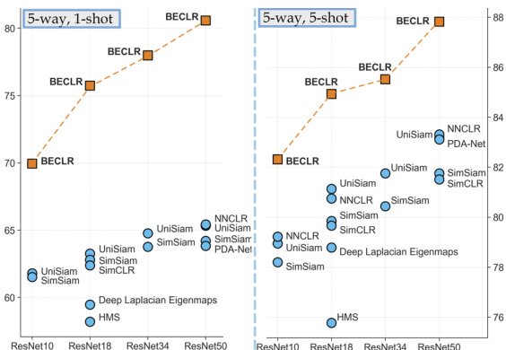
Figure 1: mini Image Net (5-way, 1-shot, left) and (5-way, 5-shot, right) accuracy in the U-FSL landscape. BECLR sets a new state-of-the-art in all settings by a significant margin.
图 1: U-FSL场景下mini Image Net的(5-way, 1-shot, 左)和(5-way, 5-shot, 右)准确率。BECLR在所有设置中以显著优势创造了新的最优性能。
The goal of pre training in U-FSL is to learn a feature extractor (a.k.a encoder) to capture the global structure of the unlabeled data. This is followed by fast adaptation of the frozen encoder to unseen tasks typically through a simple linear classifier (e.g., a logistic regression classifier). The body of literature here can be summarized into two main categories: (i) meta-learning-based pretraining where synthetic few-shot tasks resembling the downstream inference are generated for episodic training of the encoder (Hsu et al., 2018; Khodadadeh et al., 2019; 2020); (ii) (non-episodic) transferlearning approaches where pre training boils down to learning optimal representations suitable for downstream few-shot tasks (Medina et al., 2020; Chen et al., 2021b; 2022; Jang et al., 2022). Recent studies demonstrate that (more) complex meta-learning approaches are data-inefficient (Dhillon et al., 2019; Tian et al., 2020), and that the transfer-learning-based methods outperform their metalearning counterparts. More specifically, the state-of-the-art in this space is currently occupied by approaches based on contrastive learning, from the transfer-learning divide, achieving top performance across a wide variety of benchmarks (Chen et al., 2021a; Lu et al., 2022). The underlying idea of contrastive representation learning (Chen et al., 2020a; He et al., 2020) is to attract “positive” samples in the representation space while repelling “negative” ones. To efficiently materialize this, some contrastive learning approaches incorporate memory queues to alleviate the need for larger batch sizes (Zhuang et al., 2019; He et al., 2020; Dwibedi et al., 2021; Jang et al., 2022).
U-FSL中预训练的目标是学习一个特征提取器(又称编码器)以捕捉未标注数据的全局结构,随后通过简单的线性分类器(如逻辑回归分类器)快速适应未见过的任务。相关文献可归纳为两大类:(i) 基于元学习的预训练方法,通过生成模拟下游推理的合成少样本任务进行编码器的情景化训练 [Hsu et al., 2018; Khodadadeh et al., 2019; 2020];(ii) (非情景化)迁移学习方法,其预训练核心是学习适用于下游少样本任务的最优表征 [Medina et al., 2020; Chen et al., 2021b; 2022; Jang et al., 2022]。近期研究表明,(更)复杂的元学习方法存在数据低效问题 [Dhillon et al., 2019; Tian et al., 2020],而基于迁移学习的方法优于元学习方法。具体而言,当前该领域最先进的技术来自迁移学习分支中的对比学习方法,其在各类基准测试中均取得顶尖性能 [Chen et al., 2021a; Lu et al., 2022]。对比表征学习 [Chen et al., 2020a; He et al., 2020] 的核心思想是在表征空间中拉近"正样本"同时推远"负样本"。为实现这一目标,部分对比学习方法采用记忆队列来减少对大批次大小的依赖 [Zhuang et al., 2019; He et al., 2020; Dwibedi et al., 2021; Jang et al., 2022]。
Key Idea I: Going beyond instance-level contrastive learning. Operating under the unsupervised setting, contrastive FSL approaches typically enforce consistency only at the instance level, where each image within the batch and its augmentations correspond to a unique class, which is an unrealistic but seemingly unavoidable assumption. The pitfall here is that potential positive samples present within the same batch might then be repelled in the representation space, hampering the overall performance. We argue that infusing a semblance of class (or membership)-level insights into the unsupervised contrastive paradigm is essential. Our key idea to address this is extending the concept of memory queues by introducing inherent membership clusters represented by dynamically updated prototypes, while circumventing the need for large batch sizes. This enables the proposed pre training approach to sample more meaningful positive pairs owing to a novel Dynamic Clustered mEmory (DyCE) module. While maintaining a fixed memory size (same as queues), DyCE efficiently constructs and dynamically updates separable memory clusters.
关键思想一:超越实例级对比学习。在无监督设置下,对比式小样本学习方法通常仅在实例级别强制一致性,即批次中的每张图像及其增强对应一个独特类别——这种不切实际却又看似不可避免的假设存在明显缺陷:同批次内潜在的阳性样本可能在表征空间中被排斥,从而损害整体性能。我们认为,将类(或成员)层级的洞察融入无监督对比范式至关重要。为此提出的核心解决方案是通过动态更新的原型(prototype)来表示固有成员簇,从而扩展内存队列(memory queue)的概念,同时规避大批次需求。得益于新型动态聚类内存(DyCE)模块,这种预训练方法能够采样更具意义的阳性样本对。DyCE在保持固定内存容量(与队列相同)的同时,高效构建并动态更新可分离的内存簇。
Key Idea II: Addressing inherent sample bias in FSL. The base (pre training) and novel (inference) classes are either mutually exclusive classes of the same dataset or originate from different datasets - both scenarios are investigated in this paper (in Section 5). This distribution shift poses a significant challenge at inference time for the swift adaptation to the novel classes. This is further aggravated due to access to only a few labeled (a.k.a support) samples within the few-shot task because the support samples are typically not representative of the larger unlabeled (a.k.a query) set. We refer to this phenomenon as sample bias, highlighting that it is overlooked by most (U-)FSL baselines. To address this issue, we introduce an Optimal Transport-based distribution Alignment $(\mathrm{OpTA})$ add-on module within the supervised inference step. OpTA imposes no additional learnable parameters, yet efficiently aligns the representations of the labeled support and the unlabeled query sets, right before the final supervised inference step. Later on in Section 5, we demonstrate that these two novel modules (DyCE and $\mathrm{OpTA},$ ) are actually intertwined and amplify one another. Combining these two key ideas, we propose an end-to-end U-FSL approach coined as Batch-Enhanced Contrastive LeaRning (BECLR). Our main contributions can be summarized as follows:
关键思想二:解决小样本学习中的固有样本偏差问题。基础类(预训练)和新类(推理)要么来自同一数据集的不同类别,要么源自不同数据集——本文对这两种情况都进行了研究(见第5节)。这种分布偏移在推理时对快速适应新类构成了重大挑战。由于在小样本任务中只能访问少量带标签(即支持集)样本,而支持集样本通常无法代表更大的无标签(即查询集)数据集,这一问题进一步加剧。我们将此现象称为样本偏差,并指出大多数(无监督)小样本学习基线方法都忽略了这一点。为解决该问题,我们在监督推理步骤中引入了一个基于最优传输的分布对齐模块 $(\mathrm{OpTA})$。OpTA无需额外可学习参数,就能在最终监督推理步骤前有效对齐带标签支持集和无标签查询集的表征。第5节将证明,这两个新模块(DyCE和$\mathrm{OpTA}$)实际上相互交织并彼此增强。结合这两个关键思想,我们提出了一种端到端无监督小样本学习方法,称为批量增强对比学习(BECLR)。主要贡献可概括如下:
2 RELATED WORK
2 相关工作
Self-Supervised Learning (SSL). It has been approached from a variety of perspectives (Bales trier o et al., 2023). Deep metric learning methods (Chen et al., 2020a; He et al., 2020; Caron et al., 2020; Dwibedi et al., 2021), build on the principle of a contrastive loss and encourage similarity between semantically transformed views of an image. Redundancy reduction approaches (Zbontar et al., 2021; Bardes et al., 2021) infer the relationship between inputs by analyzing their cross-covariance matrices. Self-distillation methods (Grill et al., 2020; Chen & He, 2021; Oquab et al., 2023) pass different views to two separate encoders and map one to the other via a predictor. Most of these approaches construct a contrastive setting, where a symmetric or (more commonly) asymmetric Siamese network (Koch et al., 2015) is trained with a variant of the infoNCE(Oord et al., 2018) loss.
自监督学习 (SSL)。该领域已从多种角度进行研究 (Bales trier o et al., 2023)。深度度量学习方法 (Chen et al., 2020a; He et al., 2020; Caron et al., 2020; Dwibedi et al., 2021) 基于对比损失原理,通过鼓励图像语义变换视图之间的相似性进行学习。冗余减少方法 (Zbontar et al., 2021; Bardes et al., 2021) 通过分析输入数据的交叉协方差矩阵来推断其关系。自蒸馏方法 (Grill et al., 2020; Chen & He, 2021; Oquab et al., 2023) 将不同视图分别输入两个独立编码器,并通过预测器将一个视图映射到另一个。这些方法大多构建了对比学习框架,使用改进版infoNCE损失函数 (Oord et al., 2018) 来训练对称或(更常见的)非对称孪生网络 (Koch et al., 2015)。
Unsupervised Few-Shot Learning (U-FSL). The objective here is to pretrain a model from a large unlabeled dataset of base classes, akin to SSL, but tailored so that it can quickly generalize to unseen downstream FSL tasks. Meta-learning approaches (Lee et al., 2020; Ye et al., 2022) generate synthetic learning episodes for pre training, which mimic downstream FSL tasks. Here, PsCo (Jang et al., 2022) utilizes a student-teacher momentum network and optimal transport for creating pseudo-supervised episodes from a memory queue. Despite its elegant form, meta-learning has been shown to be data-inefficient in U-FSL (Dhillon et al., 2019; Tian et al., 2020). On the other hand, transfer-learning approaches (Li et al., 2022; Antoniou & Storkey, 2019; Wang et al., 2022a), follow a simpler non-episodic pre training, focused on representation quality. Notably, contrastive learning methods, such as PDA-Net (Chen et al., 2021a) and UniSiam (Lu et al., 2022), currently hold the state-of-the-art. Our proposed approach also operates within the contrastive learning premise, but also employs a dynamic clustered memory module (DyCE) for infusing membership/class-level insights within the instance-level contrastive framework. Here, S AMP Transfer (Shirekar et al., 2023) takes a different path and tries to ingrain implicit global membership-level insights through message passing on a graph neural network; however, the computational burden of this approach significantly hampers its performance with (and scale-up to) deeper backbones than Conv4.
无监督少样本学习 (U-FSL)。其目标是从大量无标注的基础类数据集中预训练模型,类似于自监督学习 (SSL),但需调整以适应下游未见过的少样本任务。元学习方法 [20][22] 通过生成模拟下游少样本任务的合成学习片段进行预训练。其中,PsCo [18] 采用师生动量网络和最优传输技术,从记忆队列中创建伪监督片段。尽管形式优雅,但元学习在无监督少样本场景中被证明数据效率低下 [8][28]。另一方面,迁移学习方法 [17][1][29] 采用更简单的非片段式预训练,专注于表征质量。值得注意的是,对比学习方法(如 PDA-Net [7] 和 UniSiam [19])当前保持最优性能。我们提出的方法同样基于对比学习框架,但引入了动态聚类记忆模块 (DyCE),在实例级对比框架中融入成员/类级信息。S AMP Transfer [26] 则另辟蹊径,试图通过图神经网络的消息传递机制隐式获取全局成员级信息,但该方法在超越 Conv4 的深层骨干网络中面临显著计算负担,制约其性能与扩展性。
Sample Bias in (U-)FSL. Part of the challenge in (U-)FSL lies in the domain difference between base and novel classes. To make matters worse, estimating class distributions only from a few support samples is inherently biased, which we refer to as sample bias. To address sample bias, Chen et al. (2021a) propose to enhance the support set with additional base-class images, Xu et al. (2022) project support samples farther from the task centroid, while Yang et al. (2021) use a calibrated distribution for drawing more support samples, yet all these methods are dependent on base-class characteristics. On the other hand, Ghaffari et al. (2021); Wang et al. (2022b) utilize Firth bias reduction to alleviate the bias in the logistic classifier itself, yet are prone to over-fitting. In contrast, the proposed OpTA module requires no fine-tuning and does not depend on the pre training dataset.
(U-)FSL中的样本偏差问题。(U-)FSL的部分挑战在于基类与新类之间的领域差异。更棘手的是,仅从少量支持样本估计类别分布本身存在固有偏差,我们称之为样本偏差。为解决样本偏差,Chen等 (2021a) 提出用额外的基类图像增强支持集,Xu等 (2022) 将支持样本投射到远离任务质心的位置,而Yang等 (2021) 采用校准分布来抽取更多支持样本,但这些方法都依赖于基类特性。另一方面,Ghaffari等 (2021) 和Wang等 (2022b) 利用Firth偏差缩减来缓解逻辑分类器本身的偏差,但容易过拟合。相比之下,提出的OpTA模块无需微调且不依赖预训练数据集。
3 PROBLEM STATEMENT: UNSUPERVISED FEW-SHOT LEARNING
3 问题陈述:无监督少样本 (Few-Shot) 学习
We follow the most commonly adopted setting in the literature (Chen et al., 2021a;b; Lu et al., 2022; Jang et al., 2022), which consists of: an unsupervised pre training, followed by a supervised inference (a.k.a fine-tuning) strategy. Formally, we consider a large unlabeled dataset ${\cal{D}}{\mathrm{{tr}}}={x{i}}$ of so-called “base” classes for pre training the model. The inference phase then involves transferring the model to unseen few-shot downstream tasks $\tau_{i}$ , drawn from a smaller labeled test dataset of so-called “novel” classes ${\cal{D}}{\mathrm{{tst}}}={(x{i},y_{i})}$ , with $y_{i}$ denoting the label of sample $\scriptstyle{\boldsymbol{x}}{i}$ . Each task $\tau{i}$ is composed of two parts $[S,{\mathcal{Q}}]$ : (i) the support set $s$ , from which the model learns to adapt to the novel classes, and (ii) the query set $\mathcal{Q}$ , on which the model is evaluated. The support set $\boldsymbol{\dot{S}}^{\dot{}}={x_{i}^{s},y_{i}^{s}}_{i=1}^{N K}$ is constructed by drawing $K$ labeled random samples from $N$ different classes, resulting in the so-called ( $N$ -way, $K$ -shot) setting. The query set $\mathcal{Q}={x_{j}^{q}}_{j=1}^{N Q}$ contains $N Q$ (with $Q>K)$ unlabeled samples. The base and novel classes are mutually exclusive, i.e., the distributions of $\mathcal{D}_{\mathrm{tr}}$ and $\mathcal{D}_{\mathrm{tst}}$ are different.
我们遵循文献中最常用的设置 (Chen et al., 2021a;b; Lu et al., 2022; Jang et al., 2022),包括:无监督预训练,随后是监督推理(即微调)策略。形式上,我们考虑一个大型无标签数据集 ${\cal{D}}{\mathrm{{tr}}}={x{i}}$,其中包含所谓的“基类”用于预训练模型。推理阶段则涉及将模型迁移到未见过的少样本下游任务 $\tau_{i}$,这些任务来自一个较小的带标签测试数据集 ${\cal{D}}{\mathrm{{tst}}}={(x{i},y_{i})}$,其中 $y_{i}$ 表示样本 $\scriptstyle{\boldsymbol{x}}{i}$ 的标签。每个任务 $\tau{i}$ 由两部分 $[S,{\mathcal{Q}}]$ 组成:(i) 支持集 $s$,模型从中学习适应新类;(ii) 查询集 $\mathcal{Q}$,用于评估模型性能。支持集 $\boldsymbol{\dot{S}}^{\dot{}}={x_{i}^{s},y_{i}^{s}}_{i=1}^{N K}$ 通过从 $N$ 个不同类中随机抽取 $K$ 个带标签样本构建,形成所谓的 ($N$-way, $K$-shot) 设置。查询集 $\mathcal{Q}={x_{j}^{q}}_{j=1}^{N Q}$ 包含 $N Q$(其中 $Q>K$)个无标签样本。基类和新类互斥,即 $\mathcal{D}_{\mathrm{tr}}$ 和 $\mathcal{D}_{\mathrm{tst}}$ 的分布不同。
4 PROPOSED METHOD: BECLR
4 提出的方法:BECLR
4.1 UNSUPERVISED PRE TRAINING
4.1 无监督预训练
We build the unsupervised pre training strategy of BECLR following contrastive representation learning. The core idea here is to efficiently attract “positive” samples (i.e., augmentations of the same image) in the representation space, while repelling “negative” samples. However, traditional contrastive learning approaches address this at the instance level, where each image within the batch has to correspond to a unique class (a statistically unrealistic assumption!). As a result, potential positives present within a batch might be treated as negatives, which can have a detrimental impact on performance. A common strategy to combat this pitfall (also to avoid prohibitively large batch sizes) is to use a memory queue (Wu et al., 2018; Zhuang et al., 2019; He et al., 2020). Exceptionally, PsCo (Jang et al., 2022) uses optimal transport to sample from a first-in-first-out memory queue and generate pseudo-supervised few-shot tasks in a meta-learning-based framework, whereas NNCLR (Dwibedi et al., 2021) uses a nearest-neighbor approach to generate more meaningful positive pairs in the contrastive loss. However, these memory queues are still oblivious to global memberships (i.e., class-level information) in the latent space. Instead, we propose to infuse membership/classlevel insights through a novel memory module (DyCE) within the pre training phase of the proposed end-to-end approach: BECLR. Fig. 2 provides a schematic illustration of the proposed contrastive pre training framework within BECLR, and Fig. 3 depicts the mechanics of DyCE.
我们遵循对比表征学习构建了BECLR的无监督预训练策略。其核心思想是在表征空间中高效吸引"正样本"(即同一图像的增强版本),同时排斥"负样本"。然而传统对比学习方法在实例层面处理这一问题,要求批次中每张图像对应唯一类别(这种统计假设并不现实)。这可能导致批次中潜在的正样本被误判为负样本,从而损害模型性能。常见解决方案(同时避免批次过大)是使用记忆队列(Wu等人,2018;Zhuang等人,2019;He等人,2020)。其中PsCo(Jang等人,2022)采用最优传输方法从先进先出记忆队列采样,在元学习框架中生成伪监督少样本任务;NNCLR(Dwibedi等人,2021)则通过最近邻方法在对比损失中生成更具意义的正样本对。但这些记忆队列仍未能利用潜在空间的全局成员关系(即类别级信息)。为此,我们在端到端框架BECLR的预训练阶段,创新性地通过动态类别记忆模块(DyCE)注入成员/类别级信息。图2展示了BECLR中的对比预训练框架示意图,图3则描述了DyCE的工作原理。
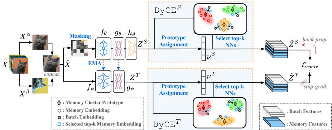
Figure 2: Overview of the proposed pre training framework of BECLR. Two augmented views of the batch images $X^{{\alpha,\beta}}$ are both passed through a student-teacher network followed by the DyCE memory module. DyCE enhances the original batch with meaningful positives and dynamically updates the memory partitions.
图 2: BECLR提出的预训练框架概述。批量图像的两个增强视图$X^{{\alpha,\beta}}$均通过师生网络传递,随后经过DyCE记忆模块处理。DyCE通过有意义的正样本增强原始批次,并动态更新记忆分区。
Pre training Strategy of BECLR. The pretraining pipeline of BECLR is summarized in Algorithm 1, and a Pytorch-like pseudo-code can be found in Appendix E. Let us now walk you through the algorithm. Let $\zeta^{a},\zeta^{b}\sim{\cal{A}}$ be two randomly sampled data augmentations from the set of all available augmentations, $\mathcal{A}$ . The minibatch can then be denoted as $\hat{\textbf{\textit{X}}}=[\hat{\textbf{\textit{x}}}{i}]{i=1}^{2B}=$ $[[\zeta^{a}({\pmb x}_{i})]_{i=1}^{B},[\zeta^{b}({\pmb x}_{i})]_{i=1}^{B}]$ , where $B$ the origi-
BECLR的预训练策略。BECLR的预训练流程总结在算法1中,类似Pytorch的伪代码可在附录E中找到。现在让我们逐步讲解该算法。设$\zeta^{a},\zeta^{b}\sim{\cal{A}}$是从所有可用增强集合$\mathcal{A}$中随机采样的两种数据增强,则小批量可表示为$\hat{\textbf{\textit{X}}}=[\hat{\textbf{\textit{x}}}{i}]{i=1}^{2B}=$$[[\zeta^{a}({\pmb x}_{i})]_{i=1}^{B},[\zeta^{b}({\pmb x}_{i})]_{i=1}^{B}]$,其中$B$为原-
Algorithm 1: Pre training of BECLR
算法1: BECLR预训练
nal batch size (line 1, Algorithm 1). As shown in Fig. 2, we adopt a student-teacher (a.k.a Siamese) asymmetric momentum architecture similar to Grill et al. (2020); Chen & He (2021). Let $\mu(\cdot)$ be a patch-wise masking operator, $f(\cdot)$ the backbone feature extractor (ResNets (He et al., 2016) in our case), and $g(\cdot),h(\cdot)$ projection and prediction multi-layer perce ptr on s (MLPs), respectively. The teacher weight parameters $(\psi)$ are an exponential moving averaged (EMA) version of the student parameters $(\theta)$ , i.e., $\psi\leftarrow m\psi+(1-m)\theta$ , as in Grill et al. (2020), where $m$ the momentum hyperparameter, while $\theta$ are updated through stochastic gradient descent (SGD). The student and teacher representations $Z^{S}$ and $\mathbf{\bar{Z}}^{T}$ (both of size $2B\times d$ , with $d$ the latent embedding dimension) can then be obtained as follows: $Z^{S}=h_{\theta}\circ g_{\theta}\circ f_{\theta}\big(\mu(\hat{X})\big)$ , $Z^{T}=g_{\psi}\circ f_{\psi}(\hat{\cal X})$ (lines 2,3).
最终批量大小(算法1第1行)。如图2所示,我们采用了与Grill等人(2020)和Chen & He(2021)类似的学生-教师(又称孪生)非对称动量架构。设$\mu(\cdot)$为逐块掩码操作符,$f(\cdot)$为骨干特征提取器(本文采用ResNets(He等人,2016)),$g(\cdot),h(\cdot)$分别为投影层和预测层的多层感知器(MLPs)。教师网络权重参数$(\psi)$是学生参数$(\theta)$的指数移动平均(EMA)版本,即$\psi\leftarrow m\psi+(1-m)\theta$,如Grill等人(2020)所述,其中$m$为动量超参数,而$\theta$通过随机梯度下降(SGD)更新。学生和教师的表征$Z^{S}$与$\mathbf{\bar{Z}}^{T}$(尺寸均为$2B\times d$,$d$为潜在嵌入维度)可通过以下方式获得:$Z^{S}=h_{\theta}\circ g_{\theta}\circ f_{\theta}\big(\mu(\hat{X})\big)$,$Z^{T}=g_{\psi}\circ f_{\psi}(\hat{\cal X})$(第2,3行)。
Upon extracting $Z^{S}$ and $Z^{T}$ , they are fed into the proposed dynamic memory module (DyCE), where enhanced versions of the batch representations $\hat{Z}^{S}$ , $\hat{Z}^{T}$ (both of size $2B(k+1)\times d$ , with $k$ denoting the number of selected nearest neighbors) are generated (line 4). Finally, we apply the contrastive loss in Eq. 3 on the enhanced batch representations $\hat{Z}^{s}$ , $\hat{Z}^{T}$ (line 5). Upon finishing unsupervised pre training, only the student encoder $\left(f_{\theta}\right)$ is kept for the subsequent inference stage.
在提取 $Z^{S}$ 和 $Z^{T}$ 后,它们被输入到提出的动态记忆模块 (DyCE) 中,生成增强版的批次表示 $\hat{Z}^{S}$ 和 $\hat{Z}^{T}$(两者大小均为 $2B(k+1)\times d$,其中 $k$ 表示所选最近邻的数量)(第4行)。最后,我们在增强的批次表示 $\hat{Z}^{s}$ 和 $\hat{Z}^{T}$ 上应用公式3中的对比损失(第5行)。完成无监督预训练后,仅保留学生编码器 $\left(f_{\theta}\right)$ 用于后续推理阶段。
Dynamic Clustered Memory (DyCE). How do we manage to enhance the batch with meaningful true positives in the absence of labels? We introduce DyCE: a novel dynamically updated clustered memory to moderate the representation space during training, while infusing a semblance of classcognizance. We demonstrate later on in Section 5 that the design choices in DyCE have a significant impact on both pre training performance as well as the downstream few-shot classification.
动态聚类内存 (DyCE)。如何在缺乏标签的情况下有效增强批次中的真实正样本?我们提出DyCE:一种新颖的动态更新聚类内存机制,在训练过程中调节表征空间,同时注入类感知特性。第5节将证明DyCE的设计选择对预训练性能和下游少样本分类均有显著影响。
Let us first establish some notation. We consider a memory unit $\mathcal{M}$ capable of storing up to $M$ latent embeddings (each of size $d$ ). To accommodate clustered memberships within DyCE, we consider up to $P$ partitions (or clusters) $\mathcal{P}{i}$ in $\mathcal{M}=[\bar{\mathcal{P}{1}},\dots,\bar{\mathcal{P}{P}}]$ , each of which is represented by a prototype stored in $\mathrm{\bfT~}=$ $[\gamma{1},\bar{\dots},\gamma_{P}]$ . Each prototype $\gamma_{i}$ (of size $1\times d$ ) is the average of the latent embeddings stored in partition $\mathcal{P}{i}$ . As shown in Fig. 3 and in Algorithm 2, DyCE consists of two informational paths: (i) the top $k$ neighbor selection and batch enhancement path (bottom branch of the figure), which uses the current state of $\mathcal{M}$ and $\mathbf{\delta}\mathbf{T}$ ; (ii) the iterative memory updating via dynamic clustering path (top branch). DyCE takes as input student or teacher embeddings (we use $Z$ here, for brevity) and returns the enhanced versions $\hat{Z}$ . We also allow for an adaptation period epoch $<\mathrm{epoch}{\mathrm{thr}}$ (empirically 20-50 epochs), during which path (i) is not activated and the training batch is not enhanced. To further elaborate, path (i) starts with assigning each $z_{i}\in Z$ to its nearest (out of $P$ ) memory prototype $\gamma_{\nu_{i}}$ based on the Euclidean distance $\langle\cdot\rangle$ . $\pmb{\nu}$ is a vector of indices (of size $2B\times1$ ) that contains these prototype assignments for all batch embeddings (line 4, Algorithm 2). Next (in line 5), we se
首先,我们建立一些符号表示。考虑一个内存单元$\mathcal{M}$,最多可存储$M$个潜在嵌入(每个大小为$d$)。为了适应DyCE中的聚类成员关系,我们在$\mathcal{M}=[\bar{\mathcal{P}{1}},\dots,\bar{\mathcal{P}{P}}]$中考虑最多$P$个分区(或聚类)$\mathcal{P}_{i}$,每个分区由存储在$\mathrm{\bfT~}=$$[\gamma_{1},\bar{\dots},\gamma_{P}]$中的原型表示。每个原型$\gamma_{i}$(大小为$1\times d$)是分区$\mathcal{P}_{i}$中存储的潜在嵌入的平均值。
如图3和算法2所示,DyCE包含两条信息路径:(i) 基于当前$\mathcal{M}$和$\mathbf{\delta}\mathbf{T}$状态的top $k$邻居选择和批次增强路径(图中下方分支);(ii) 通过动态聚类进行迭代内存更新的路径(上方分支)。DyCE接收学生或教师嵌入作为输入(为简洁起见用$Z$表示),并返回增强版本$\hat{Z}$。我们还设置了一个适应期epoch $<\mathrm{epoch}_{\mathrm{thr}}$(经验值为20-50个epoch),在此期间不激活路径(i)且不增强训练批次。
具体而言,路径(i)首先基于欧氏距离$\langle\cdot\rangle$将每个$z_{i}\in Z$分配到其最近的(在$P$个中)内存原型$\gamma_{\nu_{i}}$。$\pmb{\nu}$是一个索引向量(大小为$2B\times1$),包含所有批次嵌入的这些原型分配(算法2第4行)。接着(第5行),我们...
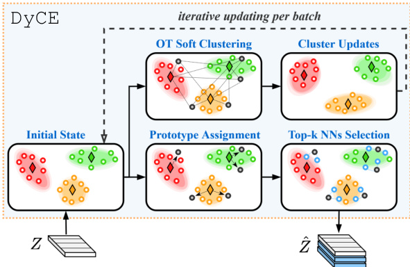
Figure 3: Overview of the proposed dynamic clustered memory (DyCE) and its two informational paths.
图 3: 提出的动态聚类记忆 (DyCE) 及其两条信息路径的概览。
Algorithm 2: DyCE
算法 2: DyCE
| ifM|=Mthen | Require: epochthr, M, T, Z, B, k |
| 2 | //路径(i): top-k与批次增强 |
| 3 | if epoch ≥ epochthr then |
| 4 | |
| 5 | j∈[P] Y←top-k({z,Pv,}),Vi∈[2B] |
| 6 | Z=[Z,Y1,...,Y2B] |
| 7 | //路径(ii):迭代式记忆更新 |
| 8 | 在Z,F间寻找最优方案:π*Solve Eq. 2 |
| 9 | 用新Z更新M:M←update(M,π*,Z) |
| 10 11 else | 丢弃最旧的2B批次嵌入: dequeue(M) |
| 12 Return:Z | 存储新批次:M←store(M,Z) |
lect the $k$ most similar memory embeddings to $z_{i}$ from the memory partition corresponding to its assigned prototype $(\mathcal{P}{\nu{i}})$ and store them in $Y_{i}$ (of size $k\times d)$ . Finally (in line 6), all $Y_{i},\forall i\in[2B]$ are concatenated into the enhanced batch $\hat{Z}=[Z,Y_{1},...,Y_{2B}]$ of size $L\times d$ (where $L=2B(k+1))$ . Path (ii) addresses the iterative memory updating by casting it into an optimal transport problem (Cuturi, 2013) given by:
从与其分配原型 $(\mathcal{P}{\nu{i}})$ 对应的内存分区中选取与 $z_{i}$ 最相似的 $k$ 个内存嵌入,并将它们存储在 $Y_{i}$ (大小为 $k\times d$) 中。最后(第6行),所有 $Y_{i},\forall i\in[2B]$ 被拼接成增强批次 $\hat{Z}=[Z,Y_{1},...,Y_{2B}]$,其大小为 $L\times d$ (其中 $L=2B(k+1))$。路径(ii)通过将其转化为最优传输问题(Cuturi, 2013)来解决迭代内存更新,该问题由以下公式给出:

to find a transport plan $\pi$ (out of $\mathbf{II}$ ) mapping $Z$ to $\mathbf{\delta}\mathbf{T}$ . Here, $\pmb{r}\in\mathbb{R}^{2B}$ denotes the distribution of batch embeddings $[z_{i}]{i=1}^{2B}$ , $\pmb{c}\in\mathbb{R}^{P}$ is the distribution of memory cluster prototypes $[\gamma{i}]_{i=1}^{P}$ . The last two conditions in Eq. 1 enforce equipartition ing (i.e., uniform assignment) of $Z$ into the $P$ memory partitions/clusters. Obtaining the optimal transport plan, $\pi^{\star}$ , can then be formulated as:
寻找一个运输计划 $\pi$(从 $\mathbf{II}$ 中选出),将 $Z$ 映射到 $\mathbf{\delta}\mathbf{T}$。这里,$\pmb{r}\in\mathbb{R}^{2B}$ 表示批次嵌入 $[z_{i}]{i=1}^{2B}$ 的分布,$\pmb{c}\in\mathbb{R}^{P}$ 是内存聚类原型 $[\gamma{i}]_{i=1}^{P}$ 的分布。式1中的最后两个条件强制实现了 $Z$ 在 $P$ 个内存分区/聚类中的均衡分配(即均匀分配)。获得最优运输计划 $\pi^{\star}$ 可以表述为:

and solved using the Sinkhorn-Knopp (Cuturi, 2013) algorithm (line 8). Here, $D$ is a pairwise distance matrix between the elements of $Z$ and $\mathbf{\delta}\mathbf{T}$ (of size $2B\times P$ ), $\langle\cdot\rangle{F}$ denotes the Frobenius dot product, $\varepsilon$ is a regular is ation term, and $\mathbb{H}(\cdot)$ is the Shannon entropy. Next (in line 9), we add the embeddings of the current batch $Z$ to $\mathcal{M}$ and use $\pi^{\star}$ for updating the partitions $\mathcal{P}_{i}$ and prototypes $\mathbf{\delta}\mathbf{T}$ (using EMA for updating). Finally, we discard the $2B$ oldest memory embeddings (line 10).
并使用 Sinkhorn-Knopp (Cuturi, 2013) 算法求解 (第 8 行)。其中,$D$ 是 $Z$ 和 $\mathbf{\delta}\mathbf{T}$ (大小为 $2B\times P$) 元素之间的成对距离矩阵,$\langle\cdot\rangle{F}$ 表示 Frobenius 点积,$\varepsilon$ 是正则化项,$\mathbb{H}(\cdot)$ 为香农熵。接着 (第 9 行),我们将当前批次的嵌入 $Z$ 添加到 $\mathcal{M}$ 中,并利用 $\pi^{\star}$ 更新分区 $\mathcal{P}_{i}$ 和原型 $\mathbf{\delta}\mathbf{T}$ (采用 EMA 更新)。最后,我们丢弃 $2B$ 个最旧的内存嵌入 (第 10 行)。
Loss Function. The popular infoNCE loss (Oord et al., 2018) is the basis of our loss function, yet recent studies (Poole et al., 2019; Song & Ermon, 2019) have shown that it is prone to high bias, when the batch size is small. To address this, we adopt a variant of infoNCE, which maximizes the same mutual information objective, but has been shown to be less biased (Lu et al., 2022):
损失函数。流行的infoNCE损失函数 (Oord et al., 2018) 是我们损失函数的基础,但最近的研究 (Poole et al., 2019; Song & Ermon, 2019) 表明,当批量较小时它容易产生高偏差。为解决这个问题,我们采用了infoNCE的一个变体,它在最大化相同互信息目标的同时,已被证明偏差更小 (Lu et al., 2022):
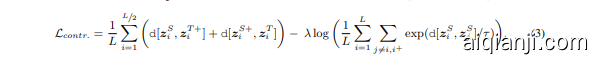
where $\tau$ is a temperature parameter, $\mathrm{d}[\cdot]$ is the negative cosine similarity, $\lambda$ is a weighting hyperparameter, $L$ is the enhanced batch size and $z_{i}^{+}$ stands for the latent embedding of the positive sample,
其中 $\tau$ 是温度参数,$\mathrm{d}[\cdot]$ 表示负余弦相似度,$\lambda$ 是加权超参数,$L$ 为增强后的批次大小,$z_{i}^{+}$ 代表正样本的潜在嵌入向量。
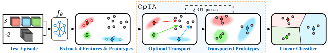
Figure 4: Overview of the inference strategy of BECLR. Given a test episode, the support $(S)$ and query $(\mathcal{Q})$ sets are passed to the pretrained feature extractor $\left(f_{\theta}\right)$ . OpTA aligns support prototypes and query features.
图 4: BECLR的推理策略概述。给定测试片段时,支持集$(S)$和查询集$(\mathcal{Q})$会被输入预训练特征提取器$\left(f_{\theta}\right)$。OpTA负责对齐支持原型和查询特征。
corresponding to sample $i$ . Following (Chen & He, 2021), to further boost training performance, we pass both views through both the student and the teacher. The first term in Eq. 3 operates on positive pairs, and the second term pushes each representation away from all other batch representations.
对应于样本$i$。遵循(Chen & He, 2021)的方法,为了进一步提升训练性能,我们将两个视图同时通过学生和教师网络。公式3中的第一项作用于正样本对,第二项则将每个表征推离批次中所有其他表征。
4.2 SUPERVISED INFERENCE
4.2 监督推理
Supervised inference (a.k.a fine-tuning) usually combats the distribution shift between training and test datasets. However, the limited number of support samples (in FSL tasks) at test time leads to a significant performance degradation due to the so-called sample bias (Cui & Guo, 2021; Xu et al., 2022). This issue is mostly disregarded in recent state-of-the-art U-FSL baselines (Chen et al., 2021a; Lu et al., 2022; Hu et al., 2023a). As part of the inference phase of BECLR, we propose a simple, yet efficient, add-on module (coined as OpTA) for aligning the distributions of the query $(\mathcal{Q})$ and support $(S)$ sets, to structurally address sample bias. Notice that $\mathrm{OpTA}$ is not a learnable module and that there are no model updates nor any fine-tuning involved in the inference stage of BECLR.
监督式推理(又称微调)通常用于应对训练集与测试集之间的分布偏移。然而在少样本学习(FSL)任务中,测试时有限的支撑样本量会因所谓的样本偏差(Cui & Guo, 2021; Xu et al., 2022)导致性能显著下降。当前最先进的U-FSL基线方法(Chen et al., 2021a; Lu et al., 2022; Hu et al., 2023a)大多忽视了这一问题。作为BECLR推理阶段的一部分,我们提出了一个简单高效的附加模块(命名为OpTA),通过对齐查询集$(\mathcal{Q})$与支撑集$(S)$的分布来结构化解决样本偏差问题。需注意$\mathrm{OpTA}$并非可学习模块,且BECLR推理阶段不涉及任何模型更新或微调操作。
Optimal Transport-based Distribution Alignment $(\tt O p T A)$ . Let $\tau=s\cup\mathcal{Q}$ be a downstream few-shot task. We first extract the support $Z^{\widetilde{S}}=f_{\theta}(S)$ (of size $N K\times d)$ and query $Z^{\mathcal{Q}}=f_{\boldsymbol{\theta}}(\mathcal{Q})$ (of size $N Q\times d)$ embeddings and calculate the support set prototypes ${\dot{P}}^{s}$ (class averages of size $N\times d)$ . Next, we find the optimal transport plan $(\pi^{\star})$ between $\mathbf{\nabla}\cdot\dot{\mathbf{\nabla}}\dot{P}^{S}$ and $Z^{\mathcal{Q}}$ using Eq. 2, with $\pmb{r}\in\mathbb{R}^{N Q}$ the distribution of $\dot{Z^{\mathcal{Q}}}$ and $\pmb{c}\in\dot{\mathbb{R}}^{N}$ the distribution of $P^{S}$ . Finally, we use $\pi^{\star}$ to map the support set prototypes onto the region occupied by the query embeddings:
基于最优传输的分布对齐 (OpTA)。设 $\tau=s\cup\mathcal{Q}$ 为一个下游少样本任务。我们首先提取支持集 $Z^{\widetilde{S}}=f_{\theta}(S)$ (尺寸为 $N K\times d$) 和查询集 $Z^{\mathcal{Q}}=f_{\boldsymbol{\theta}}(\mathcal{Q})$ (尺寸为 $N Q\times d$) 的嵌入表示,并计算支持集原型 ${\dot{P}}^{s}$ (类别平均向量,尺寸为 $N\times d$)。接着,我们利用公式2在 $\mathbf{\nabla}\cdot\dot{\mathbf{\nabla}}\dot{P}^{S}$ 和 $Z^{\mathcal{Q}}$ 之间找到最优传输方案 $(\pi^{\star})$,其中 $\pmb{r}\in\mathbb{R}^{N Q}$ 表示 $\dot{Z^{\mathcal{Q}}}$ 的分布,$\pmb{c}\in\dot{\mathbb{R}}^{N}$ 表示 $P^{S}$ 的分布。最后,我们使用 $\pi^{\star}$ 将支持集原型映射到查询嵌入所占据的区域:

where $\hat{\pi}^{\star}$ is the normalized transport plan and $\hat{P}^{S}$ are the transported support prototypes. Finally, we fit a logistic regression classifier on $\hat{P}^{S}$ to infer on the unlabeled query set. We show in Section 5 that $\mathrm{Op}\mathrm{TA}$ successfully minimizes the distribution shift (between support and query sets) and contributes to the overall significant performance margin BECLR offers against the best existing baselines. Note that we iterative ly perform $\delta$ consecutive passes of $\mathrm{OpTA}$ , where $\hat{P}^{S}$ acts as the input of the next pass. Notably, $\mathrm{Op}\mathrm{TA}$ can straightforwardly be applied on top of any U-FSL approach. An overview of $\mathrm{Op}\mathrm{TA}$ and the proposed inference strategy is illustrated in Fig. 4.
其中 $\hat{\pi}^{\star}$ 是归一化的传输方案,$\hat{P}^{S}$ 是传输后的支持原型。最后,我们在 $\hat{P}^{S}$ 上拟合一个逻辑回归分类器,以推断未标注的查询集。第5节将展示 $\mathrm{Op}\mathrm{TA}$ 成功最小化了(支持集与查询集之间的)分布偏移,并为BECLR相对于现有最佳基线带来的显著性能优势做出了贡献。需要注意的是,我们迭代执行 $\delta$ 次连续的 $\mathrm{OpTA}$ 操作,其中 $\hat{P}^{S}$ 作为下一次操作的输入。值得注意的是,$\mathrm{Op}\mathrm{TA}$ 可以直接应用于任何U-FSL方法之上。图4展示了 $\mathrm{Op}\mathrm{TA}$ 及所提出推理策略的概览。
Remark: OpTA operates on two distributions and relies on the total number of unlabeled query samples being larger than the total number of labeled support samples $(|\mathcal{Q}|>|S|)$ for reasonable distribution mapping, which is also the standard convention in the U-FSL literature. That said, $\mathrm{OpTA}$ would still perform on imbalanced FSL tasks as long as the aforementioned condition is met.
备注:OpTA 操作于两个分布之上,并依赖于未标记查询样本总数大于已标记支持样本总数 $(|\mathcal{Q}|>|S|)$ 以实现合理的分布映射,这也是 U-FSL 文献中的标准惯例。也就是说,只要满足上述条件,$\mathrm{OpTA}$ 仍可在不平衡的 FSL 任务中运行。
5 EXPERIMENTS
5 实验
In this section, we rigorously study the performance of the proposed approach both quantitatively as well as qualitatively by addressing the following three main questions:
在本节中,我们通过回答以下三个主要问题,对所提出方法的性能进行了严格的定量和定性研究:
[Q1] How does BECLR perform against the state-of-the-art for in-domain and cross-domain settings? [Q2] Does DyCE affect pre training performance by establishing separable memory partitions? [Q3] Does OpTA address the sample bias via the proposed distribution alignment strategy?
[Q1] BECLR 在领域内和跨领域设置中相比当前最优方法表现如何?
[Q2] DyCE 是否通过建立可分离的记忆分区影响预训练性能?
[Q3] OpTA 是否通过提出的分布对齐策略解决了样本偏差问题?
We use PyTorch (Paszke et al., 2019) for all implementations. Elaborate implementation and training details are discussed in the supplementary material, in Appendix A.
我们使用 PyTorch (Paszke et al., 2019) 进行所有实现。详细的实现和训练细节在补充材料的附录 A 中讨论。
Benchmark Datasets. We evaluate BECLR in terms of its in-domain performance on the two most widely adopted few-shot image classification datasets: mini Image Net (Vinyals et al., 2016) and tiered Image Net (Ren et al., 2018). Additionally, for the in-domain setting, we also evaluate on two curated versions of CIFAR-100 (Krizhevsky et al., 2009) for FSL, i.e., CIFAR-FS and FC100. Next, we evaluate BECLR in cross-domain settings on the Caltech-UCSD Birds (CUB) dataset (Welinder et al., 2010) and a more recent cross-domain FSL (CDFSL) benchmark (Guo et al., 2020). For crossdomain experiments, mini Image Net is used as the pre training (source) dataset and ChestX (Wang et al., 2017), ISIC (Codella et al., 2019), EuroSAT (Helber et al., 2019) and Crop Diseases (Mohanty et al., 2016) (in Table 3) and CUB (in Table 12 in the Appendix), as the inference (target) datasets.
基准数据集。我们在两个最广泛采用的少样本图像分类数据集上评估BECLR的域内性能:mini ImageNet (Vinyals et al., 2016) 和 tiered ImageNet (Ren et al., 2018)。此外,对于域内设置,我们还评估了针对FSL定制的两个CIFAR-100 (Krizhevsky et al., 2009)版本,即CIFAR-FS和FC100。接着,我们在跨域设置下评估BECLR,使用Caltech-UCSD Birds (CUB)数据集 (Welinder et al., 2010) 和较新的跨域FSL (CDFSL)基准 (Guo et al., 2020)。对于跨域实验,mini ImageNet被用作预训练(源)数据集,而ChestX (Wang et al., 2017)、ISIC (Codella et al., 2019)、EuroSAT (Helber et al., 2019) 和 Crop Diseases (Mohanty et al., 2016)(表3中)以及CUB(附录表12中)作为推理(目标)数据集。
Table 1: Accuracies (in $%\pm\mathrm{std})$ on mini Image Net and tiered Image Net compared against unsupervised (Unsup.) and supervised (Sup.) baselines. Backbones: RN: Residual network.†: denotes our reproduction. ∗: denotes extra synthetic training data used. Style: best and second best.
表 1: 在 miniImageNet 和 tieredImageNet 上与无监督 (Unsup.) 和有监督 (Sup.) 基线方法对比的准确率 (单位: $%\pm\mathrm{std}$)。主干网络: RN: 残差网络。†: 表示我们的复现结果。∗: 表示使用了额外的合成训练数据。样式: 最优和次优结果。
| 方法 | 主干网络 | 设置 | 5-way 1-shot | 5-way 5-shot | 5-way 1-shot | 5-way 5-shot |
|---|---|---|---|---|---|---|
| SwAVf (Caron et al., 2020) | RN18 | Unsup. | 59.84 ± 0.52 | 78.23 ± 0.26 | 65.26 ± 0.53 | 81.73 ± 0.24 |
| NNCLR (Dwibedi et al., 2021) | RN18 | Unsup. | 63.33 ± 0.53 | 80.75 ± 0.25 | 65.46 ± 0.55 | 81.40 ± 0.27 |
| CPNWCP (Wang et al., 2022a) | RN18 | Unsup. | 53.14 ± 0.62 | 67.36 ± 0.5 | 45.00 ± 0.19 | 62.96 ± 0.19 |
| HMS (Ye et al., 2022) | RN18 | Unsup. | 58.20 ± 0.23 | 75.77 ± 0.16 | 58.42 ± 0.25 | 75.85 ± 0.18 |
| SAMPTransfer (Shirekar et al., 2023) | RN18 | Unsup. | 45.75 ± 0.77 | 68.33 ± 0.66 | 42.32 ± 0.75 | 53.45 ± 0.76 |
| PsCo (Jang et al., 2022) | RN18 | Unsup. | 47.24 ± 0.76 | 65.48 ± 0.68 | 54.33 ± 0.54 | 69.73 ± 0.49 |
| UniSiam + dist (Lu et al., 2022) | RN18 | Unsup. | 64.10 ± 0.36 | 82.26 ± 0.25 | 67.01 ± 0.39 | 84.47 ± 0.28 |
| Meta-DM+UniSiam+dist* (Hu et al., 2023a) | RN18 | Unsup. | 65.64 ± 0.36 | 83.97 ± 0.25 | 67.11 ± 0.40 | 84.39 ± 0.28 |
| MetaOptNet (Lee et al., 2019) | RN18 | Sup. | 64.09 ± 0.62 | 80.00 ± 0.45 | 65.99 ± 0.72 | 81.56 ± 0.53 |
| Transductive CNAPS (Bateni et al., 2022) | RN18 | Sup. | 55.60 ± 0.90 | 73.10 ± 0.70 | 65.90 ± 1.10 | 81.80 ± 0.70 |
| BECLR (Ours) | RN18 | Unsup. | 75.74 ± 0.62 | 84.93 ± 0.33 | 76.44 ± 0.66 | 84.85 ± 0.37 |
| PDA-Net (Chen et al., 2021a) | RN50 | Unsup. | 63.84 ± 0.91 | 83.11 ± 0.56 | 69.01 ± 0.93 | 84.20 ± 0.69 |
| UniSiam + dist (Lu et al., 2022) | RN50 | Unsup. | 65.33 ± 0.36 | 83.22 ± 0.24 | 69.60 ± 0.38 | 86.51 ± 0.26 |
| Meta-DM+UniSiam + dist* (Hu et al., 2023a) | RN50 | Unsup. | 66.68 ± 0.36 | 85.29 ± 0.23 | 69.61 ± 0.38 | 86.53 ± 0.26 |
| BECLR (Ours) | RN50 | Unsup. | 80.57 ± 0.57 | 87.82 ± 0.29 | 81.69 ± 0.61 | 87.86 ± 0.32 |
Table 3: Accuracies (in $%$ ± std) on mini Image Net $\rightarrow$ CDFSL. †: our reproduc. Style: best and second best.
表 3: mini Image Net → CDFSL 上的准确率 (单位: $%$ ± 标准差)。†: 我们的复现结果。样式: 最佳与次佳结果。
| 方法 | ChestX 5-way 5-shot | ChestX 5-way 20-shot | ISIC 5-way 5-shot | ISIC 5-way 20-shot | EuroSAT 5-way 5-shot | EuroSAT 5-way 20-shot | CropDiseases 5-way 5-shot | CropDiseases 5-way 20-shot |
|---|---|---|---|---|---|---|---|---|
| SwAV+ (Caron et al., 2020) | 25.70 ± 0.28 | 30.41 ± 0.25 | 40.69 ± 0.34 | 49.03 ± 0.30 | 84.82 ± 0.24 | 90.77 ± 0.26 | 88.64 ± 0.26 | 95.11 ± 0.21 |
| NNCLR (Dwibedi et al., 2021) | 25.74 ± 0.41 | 29.54 ± 0.45 | 38.85 ± 0.56 | 47.82 ± 0.53 | 83.45 ± 0.57 | 90.80 ± 0.39 | 90.76 ± 0.57 | 95.37 ± 0.37 |
| SAMPTransfer (Shirekar et al., 2023) | 26.27 ± 0.44 | 34.15 ± 0.50 | 47.60 ± 0.59 | 61.28 ± 0.56 | 85.55 ± 0.60 | 88.52 ± 0.50 | 91.74 ± 0.55 | 96.36 ± 0.28 |
| PsCo (Jang et al., 2022) | 24.78 ± 0.23 | 27.69 ± 0.23 | 44.00 ± 0.30 | 54.59 ± 0.29 | 81.08 ± 0.35 | 87.65 ± 0.28 | 88.24 ± 0.31 | 94.95 ± 0.18 |
| UniSiam + dist (Lu et al., 2022) | 28.18 ± 0.45 | 34.58 ± 0.46 | 45.65 ± 0.58 | 56.54 ± 0.50 | 86.53 ± 0.47 | 93.24 ± 0.30 | 92.05 ± 0.50 | 96.83 ± 0.27 |
| ConFeSS (Das et al., 2021) | 27.09 | 33.57 | 48.85 | 60.10 | 84.65 | 90.40 | 88.88 | 95.34 |
| BECLR (Ours) | 28.46 ± 0.23 | 34.21 ± 0.25 | 44.48 ± 0.31 | 56.89 ± 0.29 | 88.55 ± 0.23 | 93.92 ± 0.14 | 93.65 ± 0.25 | 97.72 ± 0.13 |
5.1 EVALUATION RESULTS
5.1 评估结果
We report test accuracies with $95%$ confidence intervals over 2000 test episodes, each with $Q=15$ query shots per class, for all datasets, as is most commonly adopted in the literature (Chen et al., 2021a; 2022; Lu et al., 2022). The performance on mini Image Net, tiered Image Net, CIFAR-FS, FC100 and mini Image Net $\rightarrow\mathrm{CUB}$ is evaluated on (5-way, ${1,5}$ -shot) classification tasks, whereas for mini Image Net $\rightarrow$ CDFSL we test on (5-way, ${5,20}$ -shot) tasks, as is customary across the literature (Guo et al., 2020; Ericsson et al., 2021). We assess BECLR’s performance against a wide variety of baselines ranging from (i) established SSL baselines (Chen et al., 2020a; Grill et al., 2020; Caron et al., 2020; Zbontar et al., 2021; Chen & He, 2021; Dwibedi et al., 2021) to (ii) state-of-the- art U-FSL approaches (Chen et al., 2021a; Lu et al., 2022; Shirekar et al., 2023; Chen et al., 2022; Hu et al., 2023a; Jang et al., 2022), as well as (iii) against a set of competitive supervised baselines (Rusu et al., 2018; Gidaris et al., 2019; Lee et al., 2019; Bateni et al., 2022).
我们报告了所有数据集在2000个测试片段上95%置信区间的测试准确率,每个类别包含Q=15个查询样本( query shots ),这是文献中最常用的设置 (Chen et al., 2021a; 2022; Lu et al., 2022)。在mini ImageNet、tiered ImageNet、CIFAR-FS、FC100和mini ImageNet→CUB上的性能评估采用(5-way, {1,5}-shot)分类任务,而对于mini ImageNet→CDFSL则按照文献惯例测试(5-way, {5,20}-shot)任务 (Guo et al., 2020; Ericsson et al., 2021)。我们将BECLR的性能与多种基线方法进行比较,包括:(i) 成熟的自监督学习基线 (Chen et al., 2020a; Grill et al., 2020; Caron et al., 2020; Zbontar et al., 2021; Chen & He, 2021; Dwibedi et al., 2021),(ii) 最先进的未知域少样本学习(U-FSL)方法 (Chen et al., 2021a; Lu et al., 2022; Shirekar et al., 2023; Chen et al., 2022; Hu et al., 2023a; Jang et al., 2022),以及(iii) 一系列有竞争力的监督学习基线 (Rusu et al., 2018; Gidaris et al., 2019; Lee et al., 2019; Bateni et al., 2022)。
[A1-a] In-Domain Setting. The results for mini Image Net and tiered Image Net in the (5-way, ${1,5}$ -shot) settings are reported in Table 1. Regardless of backbone depth, BECLR sets a new state-of-the-art on both datasets, showing up to a $14%$ and $2.5%$ gain on mini Image Net over the prior art of U-FSL for the 1 and 5-shot settings, respectively. The results on tiered
[A1-a] 域内设定。表1报告了mini ImageNet和tiered ImageNet在(5-way, ${1,5}$-shot)设定下的结果。无论主干网络深度如何,BECLR在两个数据集上都创造了新的最优性能,在1-shot和5-shot设定下分别比U-FSL现有技术提升了$14%$和$2.5%$。tiered ImageNet上的结果...
Table 2: Accuracies in $(%\pm\mathrm{std})$ on CIFAR-FS and FC100 in (5-way, ${1,5}$ -shot). Style: best and second best.
表 2: CIFAR-FS 和 FC100 在 (5-way, ${1,5}$-shot) 设置下的准确率 $(%\pm\mathrm{std})$。样式: 最佳和次佳结果。
| 方法 | CIFAR-FS 1-shot | CIFAR-FS 5-shot | FC100 1-shot | FC100 5-shot |
|---|---|---|---|---|
| SimCLR (Chen et al., 2020a) | 54.56 ± 0.19 | 71.19 ± 0.18 | 36.20 ± 0.70 | 49.90 ± 0.70 |
| MoCov2 (Chen et al., 2020b) | 52.73 ± 0.20 | 67.81 ± 0.19 | 37.70 ± 0.70 | 53.20 ± 0.70 |
| LF2CS (Li et al., 2022) | 55.04 ± 0.72 | 70.62 ± 0.57 | 37.20 ± 0.70 | 52.80 ± 0.60 |
| Barlow Twins (Zbontar et al., 2021) | - | - | 37.90 ± 0.70 | 54.10 ± 0.60 |
| HMS (Ye et al., 2022) | 54.65 ± 0.20 | 73.70 ± 0.18 | 37.88 ± 0.16 | 53.68 ± 0.18 |
| Deep Eigenmaps (Chen et al., 2022) | - | - | 39.70 ± 0.70 | 57.90 ± 0.70 |
| BECLR (Ours) | 70.39 ± 0.62 | 81.56 ± 0.39 | 45.21 ± 0.50 | 60.02 ± 0.43 |
ImageNet also highlight a considerable performance margin. Interestingly, BECLR even outperforms U-FSL baselines trained with extra (synthetic) training data, sometimes distilled from deeper backbones, also the cited supervised baselines. Table 2 provides further insights on (the less commonly adopted) CIFAR-FS and FC100 benchmarks, showing a similar trend with up to $15%$ and $8%$ in 1 and 5-shot settings, respectively, for CIFAR-FS, and $5.{\bar{5}}%$ and $2%$ for FC100.
ImageNet也显示出显著的性能差距。有趣的是,BECLR甚至优于使用额外(合成)训练数据训练的U-FSL基线模型(这些数据有时从更深的主干网络蒸馏而来),同时也超越了引用的监督基线。表2提供了关于(较少采用的)CIFAR-FS和FC100基准测试的进一步分析,结果显示相似趋势:在CIFAR-FS的1样本和5样本设置中分别最高提升15%和8%,在FC100中分别提升5.5̅%和2%。
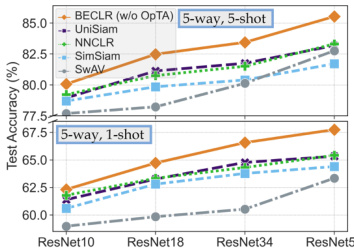
Figure 5: BECLR outperforms all baselines, in terms of U-FSL performance on mini Image Net, even without OpTA.
图 5: 即使不使用OpTA,BECLR在mini Image Net上的U-FSL(无监督少样本学习)性能也优于所有基线方法。
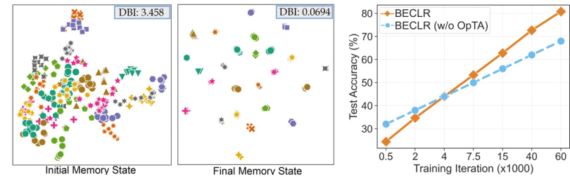
Figure 6: The dynamic updates of DyCE Figure 7: OpTA produces allow the memory to evolve into a highly an increasingly larger perforseparable partitioned latent space. Clusters mance boost as the pretrainare denoted by different (colors, markers). ing feature quality increases.
图 6: DyCE 的动态更新
图 7: OpTA 通过预训练特征质量提升,使记忆逐步演化为高度可分离的分区潜在空间,并持续产生更大的性能提升。聚类通过不同 (颜色、标记) 进行区分。
[A1-b] Cross-Domain Setting. Following Guo et al. (2020), we pretrain on mini Image Net and evaluate on CDFSL, the results of which are summarized in Tables 3. BECLR again sets a new state-of-the-art on ChestX, EuroSAT, and Crop Diseases, and remains competitive on ISIC. Notably, the data distributions of ChestX and ISIC are considerably different from that of mini Image Net. We argue that this influences the embedding quality for the downstream inference, and thus, the efficacy of OpTA in addressing sample bias. Extended versions of Tables 1-3 are found in Appendix C.
[A1-b] 跨域设置。遵循 Guo 等人 (2020) 的方法,我们在 mini Image Net 上进行预训练并在 CDFSL 上评估,结果总结在表 3 中。BECLR 在 ChestX、EuroSAT 和 Crop Diseases 上再次创造了新的最优性能,并在 ISIC 上保持竞争力。值得注意的是,ChestX 和 ISIC 的数据分布与 mini Image Net 有显著差异。我们认为这会影响下游推理的嵌入质量,从而影响 OpTA 解决样本偏差的效果。表 1-3 的扩展版本见附录 C。
Table 4: BECLR outperforms enhanced prior art with $\mathrm{OpTA}$ .
表 4: BECLR 在使用 $\mathrm{OpTA}$ 时优于现有增强方法
| 方法 | minilmageNet 1shot | minilmageNet 5shot | tieredImageNet 1shot | tieredImageNet 5shot |
|---|---|---|---|---|
| CPNWCP+OpTA (Wang et al., 2022a) | 60.45 ± 0.81 | 75.84 ± 0.56 | 55.05 ± 0.31 | 72.91 ± 0.26 |
| HMS+OpTA (Ye et al., 2022) | 69.85 ± 0.42 | 80.77 ± 0.35 | 71.75 ± 0.43 | 81.32 ± 0.34 |
| PsCo+OpTA (Jang et al., 2022) | 52.89 ± 0.71 | 67.42 ± 0.54 | 57.46 ± 0.59 | 70.70 ± 0.45 |
| UniSiam+OpTA (Lu et al., 2022) | 72.54 ± 0.61 | 82.46 ± 0.32 | 73.37 ± 0.64 | 73.37 ± 0.64 |
| BECLR (Ours) | 75.74 ± 0.62 | 84.93 ± 0.33 | 76.44 ± 0.66 | 84.85 ± 0.37 |
[A1-c] Pure Pre training and OpTA. To substantiate the impact of the design choices in BECLR, we compare against some of the most influential contrastive SSL approaches: SwAV, SimSiam, NNCLR, and the prior U-FSL state-of-the-art: UniSiam (Lu et al.,
[A1-c] 纯预训练与OpTA。为验证BECLR中设计选择的影响,我们对比了几种最具影响力的对比式自监督学习方法:SwAV、SimSiam、NNCLR,以及此前U-FSL领域的最先进方法UniSiam (Lu et al.,
2022), in terms of pure pre training performance, by directly evaluating the pretrained model on downstream FSL tasks (i.e., no OpTA and no fine-tuning). Fig. 5 summarizes this comparison for various network depths in the (5-way, ${1,5}$ -shot) settings on mini Image Net. BECLR again outperforms all U-FSL/SSL frameworks for all backbone configurations, even without $\mathrm{OpTA}$ . As an additional study, in Table 4 we take the opposite steps by plugging in $\mathrm{OpTA}$ on a suite of recent prior art in U-FSL. The results demonstrate two important points: (i) OpTA is in fact agnostic to the choice of pre training method, having considerable impact on downstream performance, and (ii) there still exists a margin between enhanced prior art and BECLR, corroborating that it is not just OpTA that has a meaningful effect but also DyCE and our pre training methodology.
2022年), 在纯预训练性能方面, 通过直接在下游少样本学习(FSL)任务上评估预训练模型(即不使用OpTA且不进行微调)。图5总结了在mini Image Net数据集上(5-way, ${1,5}$-shot)设置中不同网络深度的对比结果。即使没有$\mathrm{OpTA}$, BECLR在所有骨干网络配置中依然优于所有无监督少样本学习(U-FSL)/自监督学习(SSL)框架。作为补充研究, 表4我们采取了相反步骤: 在一系列近期U-FSL前沿方法中引入$\mathrm{OpTA}$。结果表明两个重要结论: (i) OpTA实际上对预训练方法的选择具有普适性, 对下游性能有显著影响; (ii) 增强后的前沿方法与BECLR之间仍存在差距, 证实不仅是OpTA, DyCE和我们的预训练方法也都具有实质性影响。
[A2] Latent Memory Space Evolution. As a qualitative demonstration, we visualize 30 memory embeddings from 25 partitions $\mathcal{P}{i}$ within DyCE for the initial (left) and final (right) state of the latent memory space $(\mathcal{M})$ . The 2-D UMAP plots in Fig. 6 provide qualitative evidence of a significant improvement in terms of cluster separation, as training progresses. To quantitatively substantiate this finding, the quality of the memory clusters is also measured by the DBI score (Davies & Bouldin, 1979), with a lower DBI indicating better inter-cluster separation and intra-cluster tightness. The DBI value is significantly lower between partitions $\mathcal{P}{i}$ in the final state of $\mathcal{M}$ , further corroborating DyCE’s ability to establish highly separable and meaningful partitions.
[A2] 潜在记忆空间演化。作为定性演示,我们可视化DyCE中25个分区$\mathcal{P}{i}$的30个记忆嵌入,分别对应潜在记忆空间$(\mathcal{M})$的初始(左)和最终(右)状态。图6中的二维UMAP图谱定性地展示了随着训练进行,聚类分离效果的显著提升。为量化验证这一发现,我们采用DBI指标(Davies & Bouldin, 1979)衡量记忆聚类质量,该值越低表明类间分离度与类内紧密度越优。最终状态$\mathcal{M}$中分区$\mathcal{P}{i}$间的DBI值显著降低,进一步证实DyCE能建立高度可分且有意义的分区。
[A3-a] Impact of $\tt O p I A$ . We visualize the UMAP projections for a randomly sampled (3-way, 1- shot) mini Image Net episode. Fig. 8 illustrates the original $P^{S}$ (left) and transported $\hat{P}^{S}$ (right) support prototypes $(\spadesuit)$ , along with the query set embeddings $\dot{Z}^{\mathcal{Q}}\left(\bullet\right)$ and their kernel density distributions (in contours). As can be seen, the original prototypes are highly biased and deviate from the latent query distributions. OpTA pushes the trans
[A3-a] $\tt O p I A$ 的影响。我们可视化了一个随机采样(3类,1样本)的mini Image Net场景的UMAP投影。图8展示了原始$P^{S}$(左)和传输后的$\hat{P}^{S}$(右)支持原型$(\spadesuit)$,以及查询集嵌入$\dot{Z}^{\mathcal{Q}}\left(\bullet\right)$及其核密度分布(等高线表示)。可以看出,原始原型存在显著偏差,偏离了潜在查询分布。OpTA推动了传

Figure 8: OpTA addresses sample bias, reducing the distribution shift between support and query sets.
图 8: OpTA解决了样本偏差问题,缩小了支持集和查询集之间的分布偏移。
ported prototypes much closer to the query distributions (contour centers), effectively diminishing sample bias, resulting in significantly higher accuracy in the corresponding episode.
导入的原型更接近查询分布(轮廓中心),有效减少了样本偏差,从而在相应片段中显著提高了准确性。
[A3-b] Relation between Pre training and Inference. OpTA operates under the assumption that the query embeddings $Z^{\mathcal{Q}}$ are representative of the actual class distributions. As such, we argue that its efficiency depends on the quality of the extracted features through the pretrained encoder.
[A3-b] 预训练与推理的关系。OpTA基于查询嵌入 $Z^{\mathcal{Q}}$ 能代表实际类别分布的假设运行。因此,我们认为其效率取决于通过预训练编码器提取的特征质量。
Table 6: Hyper parameter ablation study for mini Image Net (5-way, 5-shot) tasks. Accuracies in $(%\pm\mathrm{std})$ .
表 6: mini Image Net (5-way, 5-shot) 任务的超参数消融研究。准确率单位为 $(%\pm\mathrm{std})$。
| 掩码率 (MaskingRatio) | 准确率 | 输出维度 (Output Dim.(d)) | 准确率 | 负损失权重 (Neg.LossWeight (X)) | 准确率 | 近邻数 (#of NNs (k)) | 准确率 | 聚类数 (#of Clusters (P)) | 准确率 | 内存大小 (MemorySize(M)) | 准确率 | 内存模块配置 (MemoryModuleConfiguration) | 准确率 |
|---|---|---|---|---|---|---|---|---|---|---|---|---|---|
| 10% | 86.59 ± 0.25 | 256 | 85.16 ± 0.26 | 0.0 | 85.45 ± 0.27 | 1 | 86.58 ± 0.27 | 100 | 85.27 ± 0.24 | 2048 | 85.38 ± 0.25 | DyCE-FIFO | 84.05 ± 0.39 |
| 30% | 87.82 ± 0.29 | 512 | 87.82 ± 0.29 | 0.1 | 87.82 ± 0.29 | 3 | 87.82 ± 0.29 | 200 | 87.82 ± 0.29 | 4096 | 86.28 ± 0.29 | DyCE-kMeans | 85.37 ± 0.33 |
| 50% | 83.36 ± 0.28 | 1024 | 85.93 ± 0.31 | 0.3 | 86.33 ± 0.29 | 5 | 86.79 ± 0.26 | 300 | 85.81 ± 0.25 | 8192 | 87.82 ± 0.29 | DyCE | 87.82 ± 0.29 |
| 70% | 77.70 ± 0.20 | 2054 | 85.42 ± 0.34 | 0.5 | 85.63 ± 0.26 | 10 | 86.17 ± 0.28 | 500 | 85.45 ± 0.20 | 12288 | 85.84 ± 0.22 |
Fig. 7 assesses this hypothesis by comparing pure pre training (i.e., BECLR without OpTA) and downstream performance on mini Image Net for the (5-way, 1-shot) setting as training progresses. As can be seen, when the initial pre training performance is poor, OpTA even leads to performance degradation. On the contrary, it offers an increasingly larger boost as pre training accuracy improves. The key message here is that these two steps (pre training and inference) are highly intertwined, further enhancing the overall performance. This notion sits at the core of the BECLR design strategy.
图7通过比较纯预训练(即不带OpTA的BECLR)和在mini Image Net上(5-way, 1-shot)设置下随着训练进程的下游性能,评估了这一假设。可以看出,当初始预训练性能较差时,OpTA甚至会导致性能下降。相反,随着预训练准确率的提高,它带来的提升也越来越大。这里的关键信息是,这两个步骤(预训练和推理)高度交织,进一步提升了整体性能。这一概念是BECLR设计策略的核心。
5.2 ABLATION STUDIES
5.2 消融实验
Main Components of BECLR. Let us investigate the impact of sequentially adding in the four main components of BECLR’s end-to-end architecture: (i) masking, (ii) EMA teacher encoder, (iii) DyCE and $\mathrm{OpTA}$ . As can be seen from Table 5, when applied individually, masking degrades the performance, but when combined with EMA, it gives a slight boost $(1.5%)$ for both ${1,5}$ -shot settings.
BECLR的主要组件。让我们依次研究BECLR端到端架构中四个主要组件的影响:(i) 掩码 (masking), (ii) EMA教师编码器 (EMA teacher encoder), (iii) DyCE和$\mathrm{OpTA}$。从表5可以看出,单独应用掩码会降低性能,但与EMA结合时,在${1,5}$-少样本设置下均能带来小幅提升$(1.5%)$。
Table 5: Ablating main components of BECLR.
表 5: BECLR 主要组件的消融实验
| Masking | EMATeacher | DyCE | OpTA | 5-way1-shot | 5-way5-shot |
|---|---|---|---|---|---|
| 63.57 ± 0.43 | 81.42 ± 0.28 | ||||
| √ | 54.53 ± 0.42 | 68.35 ± 0.27 | |||
| √ | 65.02 ± 0.41 | 82.33 ± 0.25 | |||
| √ | √ | 65.33 ± 0.44 | 82.69 ± 0.26 | ||
| √ | √ | 67.75 ± 0.43 | 85.53 ± 0.27 | ||
| √ | 80.57 ± 0.57 | 87.82 ± 0.29 |
DyCE and $\mathrm{Op}\mathrm{TA}$ are the most crucial components contributing to the overall performance of BECLR. DyCE offers an extra $2.4%$ and $2.8%$ accuracy boost in the 1-shot and 5-shot settings, respectively, and $\mathrm{OpTA}$ provides another $12.8%$ and $2.3%$ performance gain, in the aforementioned settings. As discussed earlier, also illustrated in Fig. 7, the gain of $\mathrm{Op}\mathrm{TA}$ is owing and proportional to the performance of DyCE. This boost is paramount in the 1-shot scenario where the sample bias is severe.
DyCE和$\mathrm{Op}\mathrm{TA}$是提升BECLR整体性能的最关键组件。在1样本和5样本设置中,DyCE分别带来额外2.4%和2.8%的准确率提升,而$\mathrm{OpTA}$在上述场景中进一步贡献了12.8%和2.3%的性能增益。如先前讨论及图7所示,$\mathrm{Op}\mathrm{TA}$的增益与DyCE的性能呈正相关。这一提升在样本偏差严重的1样本场景中尤为重要。
Other Hyper parameters. In Table 6, we summarize the result of ablations on: (i) the masking ratio of student images, (ii) the embedding latent dimension $d$ , (iii) the loss weighting hyper parameter $\lambda$ (in Eq. 3), and regarding DyCE: (iv) the number of nearest neighbors selected $k$ , (v) the number of memory partitions/clusters $P$ , (vi) the size of the memory $M$ , and (vii) different memory module configurations. As can be seen, a random masking ratio of $30%$ yields the best performance. We find that $d=512$ gives the best results, which is consistent with the literature (Grill et al., 2020; Chen & He, 2021). The negative loss term turns out to be unnecessary to prevent representation collapse (as can be seen when $\lambda=0$ ) and $\lambda=0.1$ yields the best performance. Regarding the number of neighbors selected $(k)$ , there seems to be a sweet spot in this setting around $k=3$ , where increasing further would lead to inclusion of potentially false positives, and thus performance degradation. $P$ and $M$ are tunable hyper parameters (per dataset) that return the best performance at $P=200$ and $M=8192$ in this setting. Increasing $P$ , $M$ beyond a certain threshold appears to have a negative impact on cluster formation. We argue that extremely large memory would result in accumulating old embeddings, which might no longer be a good representative of their corresponding classes. Finally, we compare DyCE against two degenerate versions of itself: DyCE-FIFO, where the memory has no partitions and is updated with a first-in-first-out strategy; here for incoming embeddings we pick the closest $k$ neighbors. DyCE-kMeans, where we preserve the memory structure and only replace optimal transport with kMeans (with $P$ clusters), in line 8 of Algorithm 2. The performance drop in both cases confirms the importance of the proposed mechanics within DyCE.
其他超参数。表6总结了以下消融实验结果:(i) 学生图像掩码比例,(ii) 嵌入潜在维度$d$,(iii) 损失加权超参数$\lambda$(公式3),以及关于DyCE的:(iv) 最近邻选择数量$k$,(v) 内存分区/聚类数量$P$,(vi) 内存大小$M$,(vii) 不同内存模块配置。可见$30%$的随机掩码比例表现最佳。$d=512$的结果最优,这与文献[20][21]一致。负损失项对防止表征坍缩并非必需($\lambda=0$时仍有效),$\lambda=0.1$时性能最佳。关于最近邻数量$(k)$,$k=3$存在最佳平衡点,继续增大会引入误报导致性能下降。$P$和$M$是可调超参数(按数据集),本设定中$P=200$和$M=8192$时表现最优。超过阈值后继续增加$P$、$M$会对聚类形成产生负面影响。我们认为过大的内存会累积陈旧嵌入,使其无法有效代表对应类别。最后将DyCE与两个退化版本对比:DyCE-FIFO(无分区内存+先进先出更新策略,对新嵌入选取最近$k$邻)和DyCE-kMeans(保留内存结构但用kMeans替代最优传输,算法2第8行)。两种情况的性能下降证实了DyCE核心机制的重要性。
6 CONCLUDING REMARKS AND BROADER IMPACT
6 结论与更广泛的影响
In this paper, we have articulated two key shortcomings of the prior art in U-FSL, to address each of which we have proposed a novel solution embedded within the proposed end-to-end approach, BECLR. The first angle of novelty in BECLR is its dynamic clustered memory module (coined as DyCE) to enhance positive sampling in contrastive learning. The second angle of novelty is an efficient distribution alignment strategy (called OpTA) to address the inherent sample bias in (U-)FSL. Even though tailored towards U-FSL, we believe DyCE has potential broader impact on generic self-supervised learning state-of-the-art, as we already demonstrate (in Section 5) that even with OpTA unplugged, DyCE alone empowers BECLR to still outperform the likes of SwaV, SimSiam and NNCLR. OpTA, on the other hand, is an efficient add-on module, which we argue has to become an integral part of all (U-)FSL approaches, especially in the more challenging low-shot scenarios.
在本文中,我们阐述了现有U-FSL技术的两个关键缺陷,并针对每个问题在提出的端到端方法BECLR中嵌入了创新解决方案。BECLR的第一个创新点是其动态聚类记忆模块(命名为DyCE),用于增强对比学习中的正样本采样。第二个创新点是高效的分布对齐策略(称为OpTA),用于解决(U-)FSL中固有的样本偏差问题。尽管专为U-FSL设计,我们认为DyCE对通用自监督学习的前沿技术具有更广泛的影响潜力——正如我们在第5节所示:即使移除OpTA模块,仅DyCE就使BECLR性能超越SwaV、SimSiam和NNCLR等基准方法。而OpTA作为一个高效附加模块,我们主张其应成为所有(U-)FSL方法的必要组成部分,尤其在更具挑战性的少样本场景中。
REPRODUCIBILITY STATEMENT.
可复现性声明
To help readers reproduce our experiments, we provide extensive descriptions of implementation details and algorithms. Architectural and training details are provided in Appendices A.1 and A.2, respectively, along with information on the applied data augmentations (Appendix A.3) and tested benchmark datasets (Appendix B.1). The algorithms for BECLR pre training and DyCE are also provided in both algorithmic (in Algorithms 1, 2) and Pytorch-like pseudocode formats (in Algorithms 3, 4). We have taken every measure to ensure fairness in our comparisons by following the most commonly adopted pre training and evaluation settings in the U-FSL literature in terms of: pre training/inference benchmark datasets used for both in-domain and cross-domain experiments, pre training data augmentations, $N$ -way, $K$ -shot) inference settings and number of query set images per tested episode. We also draw baseline results from their corresponding original papers and compare their performance with BECLR for identical backbone depths. For our reproductions (denoted as †) of SwAV and NNCLR we follow the codebase of the original work and adopt it in the U-FSL setup, by following the same augmentations, backbones, and evaluation settings as BECLR. Our codebase is also provided as part of our supplementary material, in an anonymized fashion, and will be made publicly available upon acceptance. All training and evaluation experiments are conducted on 2 A40 NVIDIA GPUs.
为帮助读者复现实验,我们详细描述了实现细节与算法。架构设计和训练细节分别见附录A.1与A.2,同时提供了采用的数据增强方案(附录A.3)和测试基准数据集(附录B.1)。BECLR预训练与DyCE算法均以算法描述(算法1、2)和类PyTorch伪代码(算法3、4)两种形式呈现。为确保对比公平性,我们严格遵循U-FSL领域最通用的预训练与评估设置,包括:跨领域/领域内实验使用的预训练/推理基准数据集、预训练数据增强、$N$-way $K$-shot推理设置及每测试片段查询集图像数量。所有基线结果均引自原始论文,并在相同骨干网络深度下与BECLR进行性能对比。对于SwAV和NNCLR的复现(标记为†),我们基于原代码库适配U-FSL设置,采用与BECLR相同的数据增强、骨干网络及评估配置。代码库将以匿名形式作为补充材料提供,录用后公开。所有训练与评估实验均在2块NVIDIA A40 GPU上完成。
ETHICS STATEMENT.
伦理声明。
We have read the ICLR Code of Ethics (https://iclr.cc/public/Code Of Ethics) and ensured that this work adheres to it. All benchmark datasets and pretrained model checkpoints are publicly available and not directly subject to ethical concerns.
我们已阅读ICLR道德准则(https://iclr.cc/public/Code Of Ethics)并确保本工作符合该准则。所有基准数据集和预训练模型检查点均为公开可用资源,不直接涉及伦理问题。
ACKNOWLEDGEMENTS.
致谢
The authors would like to thank Marcel Reinders, Ojas Shirekar and Holger Caesar for insightful conversations and brainstorming. This work was in part supported by Shell.ai Innovation program.
作者感谢 Marcel Reinders、Ojas Shirekar 和 Holger Caesar 富有见地的讨论与头脑风暴。此项研究部分由 Shell.ai 创新计划支持。
REFERENCES
参考文献
Antreas Antoniou and Amos Storkey. Assume, augment and learn: Unsupervised few-shot metalearning via random labels and data augmentation. arXiv preprint arXiv:1902.09884, 2019.
Antreas Antoniou 和 Amos Storkey. 假设、增强与学习:通过随机标签和数据增强的无监督少样本元学习. arXiv preprint arXiv:1902.09884, 2019.
Ting Chen, Simon Kornblith, Mohammad Norouzi, and Geoffrey Hinton. A simple framework for contrastive learning of visual representations. In International conference on machine learning, pp. 1597–1607. PMLR, 2020a.
Ting Chen、Simon Kornblith、Mohammad Norouzi 和 Geoffrey Hinton。视觉表征对比学习的简单框架。见《国际机器学习会议》,第1597–1607页。PMLR,2020a。
Jean-Bastien Grill, Florian Strub, Florent Altché, Corentin Tallec, Pierre Richemond, Elena Buch at s kaya, Carl Doersch, Bernardo Avila Pires, Zhaohan Guo, Mohammad Gheshlaghi Azar, et al. Bootstrap your own latent-a new approach to self-supervised learning. Advances in neural information processing systems, 33:21271–21284, 2020.
Jean-Bastien Grill、Florian Strub、Florent Altché、Corentin Tallec、Pierre Richemond、Elena Buchatskaya、Carl Doersch、Bernardo Avila Pires、Zhaohan Guo、Mohammad Gheshlaghi Azar 等。自展潜在变量——自监督学习的新方法。神经信息处理系统进展,33:21271–21284,2020。
Aravind Rajeswaran, Chelsea Finn, Sham M Kakade, and Sergey Levine. Meta-learning with implicit gradients. Advances in neural information processing systems, 32, 2019.
Aravind Rajeswaran、Chelsea Finn、Sham M Kakade 和 Sergey Levine。基于隐式梯度的元学习。神经信息处理系统进展,32,2019。
Pietro Perona. Caltech-ucsd birds 200. 2010.
Pietro Perona. Caltech-ucsd birds 200. 2010.
A IMPLEMENTATION DETAILS
实现细节
This section describes the implementation and training details of BECLR.
本节介绍 BECLR 的实现和训练细节。
A.1 ARCHITECTURE DETAILS
A.1 架构细节
BECLR is implemented on PyTorch (Paszke et al., 2019). We use the ResNet family (He et al., 2016) for our backbone networks $(f_{\theta},f_{\psi})$ . The projection $(g_{\theta},g_{\psi})$ and prediction $(h_{\theta})$ heads are 3- and 2- layer MLPs, respectively, as in Chen & He (2021). Batch normalization (BN) and a ReLU activation function are applied to each MLP layer, except for the output layers. No ReLU activation is applied on the output layer of the projection heads $(g_{\theta},g_{\psi})$ , while neither BN nor a ReLU activation is applied on the output layer of the prediction head $(h_{\theta})$ . We use a resolution of $224\times224$ for input images and a latent embedding dimension of $d=512$ in all models and experiments, unless otherwise stated. The DyCE memory module consists of a memory unit $\mathcal{M}$ , initialized as a random table (of size $M\times d)$ . We also maintain up to $P$ partitions in $\mathcal{M}=[\mathcal{P}_{1},\dots,\mathcal{P}_{P}]$ , each of which is represented by a prototype stored in $\boldsymbol{\Gamma}=[\gamma_{1},\dots,\gamma_{P}]$ . Prototypes $\gamma_{i}$ are the average of the latent embeddings stored in partition $\mathcal{P}_{i}$ . When training on mini Image Net, CIFAR-FS and FC100, we use a memory of size $M=8192$ that contains $P=200$ partitions and cluster prototypes ( $M=40960$ , $P=1000$ for tiered Image Net). Note that both $M$ and $P$ are important hyper parameters, whose values were selected by evaluating on the validation set of each dataset for model selection. These hyper parameters would also need to be carefully tuned on an unknown unlabeled training dataset.
BECLR基于PyTorch (Paszke等人,2019)实现。主干网络$(f_{\theta},f_{\psi})$采用ResNet系列(He等人,2016)。投影头$(g_{\theta},g_{\psi})$和预测头$(h_{\theta})$分别为3层和2层MLP,遵循Chen & He (2021)的设计。除输出层外,每个MLP层均应用批归一化(BN)和ReLU激活函数。投影头$(g_{\theta},g_{\psi})$的输出层不使用ReLU激活,而预测头$(h_{\theta})$的输出层既不使用BN也不使用ReLU激活。除非特别说明,所有模型和实验均采用$224\times224$输入图像分辨率,潜在嵌入维度设为$d=512$。DyCE记忆模块包含一个随机初始化的记忆单元$\mathcal{M}$(大小为$M\times d$),并维护最多$P$个分区$\mathcal{M}=[\mathcal{P}_{1},\dots,\mathcal{P}_{P}]$,每个分区由存储在$\boldsymbol{\Gamma}=[\gamma_{1},\dots,\gamma_{P}]$中的原型表示。原型$\gamma_{i}$是分区$\mathcal{P}_{i}$内存储的潜在嵌入均值。在mini ImageNet、CIFAR-FS和FC100数据集训练时,我们设置记忆大小$M=8192$和分区数$P=200$(tiered ImageNet使用$M=40960$,$P=1000$)。需注意$M$和$P$均为重要超参数,其取值通过各数据集验证集评估确定。这些超参数在未知无标注训练数据集上也需要仔细调整。
A.2 TRAINING DETAILS
A.2 训练细节
BECLR is pretrained on the training splits of mini Image Net, CIFAR-FS, FC100 and tiered Image Net. We use a batch size of $B=256$ images for all datasets, except for tiered Image Net $\mathit{\Theta}^{\prime}B=512\$ ). Following Chen & He (2021), images are resized to $224\times224$ for all configurations. We use the SGD optimizer with a weight decay of $10^{-4}$ , a momentum of 0.995, and a cosine decay schedule of the learning rate. Note that we do not require large-batch optimizers, such as LARS (You et al., 2017), or early stopping. Similarly to Lu et al. (2022), the initial learning rate is set to 0.3 for the smaller mini Image Net, CIFAR-FS, FC100 datasets and 0.1 for tiered Image Net, and we train for 400 and 200 epochs, respectively. The temperature scalar in the loss function is set to $\tau=2$ . Upon finishing unsupervised pre training, we only keep the last epoch checkpoint of the student encoder $\left(f_{\theta}\right)$ for the subsequent inference stage. For the inference and downstream few-shot classification stage, we create ( $N$ -way, $K$ -shot) tasks from the validation and testing splits of each dataset for model selection and evaluation, respectively. In the inference stage, we sequentially perform up to $\delta\leq5$ consecutive passes of $\mathrm{Op}\mathrm{TA}$ , with the transported prototypes of each pass acting as the input of the next pass. The optimal value for $\delta$ for each dataset and $N$ -way, $K$ -shot) setting is selected by evaluating on the validation dataset.
BECLR在mini Image Net、CIFAR-FS、FC100和tiered Image Net的训练集上进行了预训练。除tiered Image Net使用批量大小$B=512$外,所有数据集均采用$B=256$的图像批量。根据Chen & He (2021)的方法,所有配置下图像尺寸调整为$224\times224$。我们使用SGD优化器,权重衰减为$10^{-4}$,动量为0.995,并采用学习率的余弦衰减调度。值得注意的是,我们不需要LARS (You et al., 2017)等大批量优化器或早停策略。与Lu et al. (2022)类似,较小规模的mini Image Net、CIFAR-FS和FC100数据集初始学习率设为0.3,tiered Image Net设为0.1,分别训练400和200个周期。损失函数中的温度系数设置为$\tau=2$。无监督预训练完成后,我们仅保留学生编码器$\left(f_{\theta}\right)$的最后周期检查点用于后续推理阶段。
在推理和下游少样本分类阶段,我们分别从各数据集的验证集和测试集创建($N$-way, $K$-shot)任务用于模型选择和评估。推理阶段会顺序执行最多$\delta\leq5$次连续$\mathrm{Op}\mathrm{TA}$运算,每次运算得到的传输原型将作为下一次运算的输入。每个数据集在($N$-way, $K$-shot)设置下的最优$\delta$值通过验证集评估确定。
Note that at the beginning of pre training both the encoder representations and the memory embedding space within DyCE are highly volatile. Thus, we allow for an adaptation period epoch $<$ $\operatorname{epoch}{\operatorname{thr}}$ (empirically 20-50 epochs), during which the batch enhancement path of DyCE is not activated and the encoder is trained via standard contrastive learning (without enhancing the batch with additional positives). On the contrary, the memory updating path of DyCE is activated for every training batch from the beginning of training, allowing the memory to reach a highly separable converged state (see Fig. 6), before plugging in the batch enhancement path in the BECLR pipeline. When the memory space $(\mathcal{M})$ is full for the first time, a kmeans (Likas et al., 2003) clustering step is performed for initializing the cluster prototypes $(\gamma{i})$ and memory partitions $(\mathcal{P}_{i})$ . This kmeans clustering step is performed only once during training to initialize the memory prototypes, which are then dynamically updated for each training batch by the memory updating path of DyCE.
需要注意的是,在预训练初期,DyCE中的编码器表示和记忆嵌入空间都具有高度不稳定性。因此,我们设置了一个适应期 epoch $<$ $\operatorname{epoch}{\operatorname{thr}}$ (经验值为20-50个epoch),在此期间不激活DyCE的批次增强路径,编码器通过标准对比学习进行训练(不通过额外正样本增强批次)。相反,从训练开始就对每个训练批次激活DyCE的记忆更新路径,使得记忆在接入BECLR流程的批次增强路径前能达到高度可分离的收敛状态(见图6)。当记忆空间 $(\mathcal{M})$ 首次填满时,会执行一次kmeans (Likas et al., 2003)聚类步骤来初始化聚类原型 $(\gamma{i})$ 和记忆分区 $(\mathcal{P}_{i})$。这个kmeans聚类步骤在训练期间仅执行一次以初始化记忆原型,随后由DyCE的记忆更新路径对每个训练批次进行动态更新。
A.3 IMAGE AUGMENTATIONS
A.3 图像增强
The data augmentations that were applied in the pre training stage of BECLR are showcased in Table 7. These augmentations were applied on the input images for all training datasets. The default data augmentation profile follows a common data augmentation strategy in SSL, including RandomResized Crop (with scale in [0.2, 1.0]), random Color J it ter (Wu et al., 2018) of {brightness, contrast, saturation, hue} with a probability of 0.1, Random GrayScale with a probability of 0.2, random Gaussian Blur with a probability of 0.5 and a Gaussian kernel in [0.1, 2.0], and finally, RandomHori zonta l Flip with a probability of 0.5. Following Lu et al. (2022), this profile can be expanded to the strong data augmentation profile, which also includes Radom Vertical Flip with a probability of 0.5 and Rand Augment (Cubuk et al., 2020) with $n=2$ layers, a magnitude of $m=10$ , and a noise of the standard deviation of magnitude of $m s t d=0.5$ . Unless otherwise stated, the strong data augmentation profile is applied on all training images before being passed to the backbone encoders.
表7展示了BECLR预训练阶段采用的数据增强方法。这些增强操作应用于所有训练数据集的输入图像。默认数据增强方案遵循自监督学习(SSL)中常见的策略,包括:随机缩放裁剪(RandomResized Crop)(缩放范围[0.2,1.0])、以0.1概率随机调整色彩(Color Jitter)(Wu等人,2018){亮度、对比度、饱和度、色调}、0.2概率随机灰度化(Random GrayScale)、0.5概率高斯模糊(Gaussian Blur)(核大小[0.1,2.0]),以及0.5概率水平翻转(RandomHorizontal Flip)。根据Lu等人(2022)的研究,该方案可扩展为强数据增强方案,新增0.5概率垂直翻转(Radom Vertical Flip)和随机增强(Rand Augment)(Cubuk等人,2020)(层数$n=2$、幅度$m=10$、噪声标准差$m std=0.5$)。除非另有说明,所有训练图像在输入主干编码器前均采用强数据增强方案。
Table 7: Pytorch-like descriptions of the data augmentation profiles applied on the pre training phase of BECLR.
表 7: BECLR 预训练阶段应用的数据增强配置的类 Pytorch 描述
| DataAugmentationProfile | Description |
|---|---|
| Default | RandomResizedCrop(size=224,scale=(0.2,1)) RandomApply([ColorJitter(brightness=0.4,contrast=0.4,saturation=0.4,hue=0.1)],p=0.1) RandomGrayScale(p=0.2) RandomApply([GaussianBlur([0.1, 2.0])], p=0.5) RandomHorizontalFlip(p=0.5) |
| Strong | RandomResizedCrop(size=224,scale=(0.2,1)) RandomApply([ColorJitter(brightness=0.4, contrast=0.4, saturation=0.2, hue=0.1)], p=0.1) RandomGrayScale(p=0.2) RandomApply([GaussianBlur([o.1,2.0])],p=0.5) RandAugment(n=2,m=10,mstd=0.5) |
B EXPERIMENTAL SETUP
B 实验设置
In this section, we provide more detailed information regarding all the few-shot benchmark datasets that were used as part of our experimental evaluation (in Section 5), along with BECLR’s training and evaluation procedures for both in-domain and cross-domain U-FSL settings, for ensuring fair comparisons with U-FSL baselines and our reproductions (for SwAV and NNCLR).
在本节中,我们将详细介绍实验评估(第5节)中使用的所有少样本基准数据集,以及BECLR在领域内和跨领域U-FSL(无监督少样本学习)设置下的训练与评估流程,以确保与U-FSL基线方法及我们的复现结果(SwAV和NNCLR)进行公平比较。
Table 8: Overview of cross-domain few-shot benchmarks, on which BECLR is evaluated. The datasets are sorted with decreasing (distribution) domain similarity to ImageNet and mini Image Net.
表 8: BECLR 评估所用的跨领域少样本基准概览。数据集按与 ImageNet 和 mini ImageNet 的(分布)领域相似度降序排列。
| ImageNet相似度 | 数据集 | 类别数 | 样本数 |
|---|---|---|---|
| High | CUB (Welinder et al., 2010) | 200 | 11,788 |
| Low | CropDiseases (Mohanty et al., 2016) | 38 | 43,456 |
| Low | EuroSAT (Helber et al., 2019) | 10 | 27,000 |
| Low | ISIC (Codella et al., 2019) | 7 | 10,015 |
| Low | ChestX (Wang et al., 2017) | 7 | 25,848 |
B.1 DATASET DETAILS
B.1 数据集详情
mini Image Net. It is a subset of ImageNet (Russ a kov sky et al., 2015), containing 100 classes with 600 images per class. We randomly select 64, 16, and 20 classes for training, validation, and testing, following the predominantly adopted settings of Ravi & Larochelle (2016).
mini ImageNet。它是ImageNet (Russakovsky et al., 2015)的一个子集,包含100个类别,每个类别有600张图像。我们按照Ravi & Larochelle (2016)主要采用的设置,随机选择64、16和20个类别分别用于训练、验证和测试。
tiered Image Net. It is a larger subset of ImageNet, containing 608 classes and a total of 779, 165 images, grouped into 34 high-level categories, 20 (351 classes) of which are used for training, 6 (97 classes) for validation and 8 (160 classes) for testing.
分层式Image Net。这是ImageNet的一个更大子集,包含608个类别共计779,165张图像,划分为34个高级类别,其中20个类别(351个类)用于训练,6个类别(97个类)用于验证,8个类别(160个类)用于测试。
CIFAR-FS. It is a subset of CIFAR-100 (Krizhevsky et al., 2009), which is focused on FSL tasks by following the same sampling criteria that were used for creating mini Image Net. It contains 100 classes with 600 images per class, grouped into 64, 16, 20 classes for training, validation, and testing, respectively. The additional challenge here is the limited original image resolution of $32\times32$ .
CIFAR-FS。它是CIFAR-100 (Krizhevsky et al., 2009) 的一个子集,通过采用与创建mini Image Net相同的采样标准,专注于少样本学习 (FSL) 任务。该数据集包含100个类别,每个类别有600张图像,分别划分为64、16、20个类别用于训练、验证和测试。其额外挑战在于原始图像分辨率有限,仅为 $32\times32$。
FC100. It is also a subset of CIFAR-100 (Krizhevsky et al., 2009) and contains the same 60000 $(32\times32)$ images as CIFAR-FS. Here, the original 100 classes are grouped into 20 super classes, in such a way as to minimize the information overlap between training, validation and testing classes (McAllester & Stratos, 2020). This makes this data set more demanding for (U-)FSL, since training and testing classes are highly dissimilar. The training split contains 12 super classes (of 60 classes), while both the validation and testing splits are composed of 4 super classes (of 20 classes).
FC100。它也是CIFAR-100 (Krizhevsky et al., 2009) 的一个子集,包含与CIFAR-FS相同的60000张 $(32\times32)$ 图像。原始100个类别被划分为20个超类,这种划分方式旨在最小化训练集、验证集和测试集类别之间的信息重叠 (McAllester & Stratos, 2020)。由于训练类和测试类差异较大,这使得该数据集对(无监督)少样本学习更具挑战性。训练集包含12个超类(共60个类别),而验证集和测试集各由4个超类(共20个类别)组成。
CDFSL. It consists of four distinct datasets with decreasing domain similarity to ImageNet, and by extension mini Image Net, ranging from crop disease images in Crop Diseases (Mohanty et al., 2016) and aerial satellite images in EuroSAT (Helber et al., 2019) to dermatological skin lesion images in ISIC2018 (Codella et al., 2019) and grayscale chest X-ray images in ChestX (Wang et al., 2017).
CDFSL。该数据集包含四个与ImageNet(以及mini ImageNet)领域相似度递减的不同数据集:从Crop Diseases (Mohanty等人, 2016)中的作物病害图像、EuroSAT (Helber等人, 2019)的航拍卫星图像,到ISIC2018 (Codella等人, 2019)的皮肤病损图像,以及ChestX (Wang等人, 2017)的灰度胸部X光图像。
CUB. It consists of 200 classes and a total of 11, 788 images, split into 100 classes for training and 50 for both validation and testing, following the split settings of Chen et al. (2018). Additional information on the cross-domain few-shot benchmarks (CUB and CDFSL) is provided in Table 8.
CUB。该数据集包含200个类别,共计11,788张图像,按照Chen等人(2018)的划分设置,分为100个训练类、50个验证类和50个测试类。跨域少样本基准测试(CUB和CDFSL)的更多信息见表8。
B.2 PRE TRAINING AND EVALUATION PROCEDURES
B.2 预训练与评估流程
For all in-domain experiments BECLR is pretrained on the training split of the selected dataset (mini Image Net, tiered Image Net, CIFAR-FS, or FC100), followed by the subsequent inference stage on the validation and testing splits of the same dataset for model selection and final evaluation, respectively. In contrast, in the cross-domain setting BECLR is pretrained on the training split of mini Image Net and then evaluated on the validation and test splits of either CDFSL (ChestX, ISIC, EuroSAT, Crop Diseases) or CUB. We report test accuracies with $95%$ confidence intervals over 2000 test episodes, each with 15 query shots per class, for all tested datasets, as is most commonly adopted in the literature (Chen et al., 2021a; 2022; Lu et al., 2022). The performance on mini Image Net, tiered Image Net, CIFAR-FS, FC100 and mini Image Net $\rightarrow\mathrm{CUB}$ is evaluated on (5-way, ${1,5}$ -shot) classification tasks, while on mini Image Net $\rightarrow\mathrm{CDFSL}$ we evaluate on (5-way, ${5,20}$ -shot) tasks, as is customary across the literature (Guo et al., 2020).
对于所有领域内实验,BECLR 在选定数据集 (mini ImageNet、tiered ImageNet、CIFAR-FS 或 FC100) 的训练集上进行预训练,随后在同一数据集的验证集和测试集上分别进行模型选择和最终评估的推理阶段。而在跨领域设置中,BECLR 先在 mini ImageNet 训练集上预训练,然后在 CDFSL (ChestX、ISIC、EuroSAT、Crop Diseases) 或 CUB 的验证集和测试集上进行评估。我们按照文献中最常见的做法 (Chen et al., 2021a; 2022; Lu et al., 2022),报告所有测试数据集在 2000 个测试 episode 上的测试准确率(每个 episode 每类包含 15 个查询样本),并附 $95%$ 置信区间。mini ImageNet、tiered ImageNet、CIFAR-FS、FC100 和 mini ImageNet $\rightarrow\mathrm{CUB}$ 的性能评估采用 (5-way, ${1,5}$-shot) 分类任务,而 mini ImageNet $\rightarrow\mathrm{CDFSL}$ 则按照文献惯例 (Guo et al., 2020) 采用 (5-way, ${5,20}$-shot) 任务进行评估。
We have taken every measure to ensure fairness in our comparison with U-FSL baselines and our reproductions. To do so, all compared baselines have the same pre training and testing dataset (in both in-domain and cross-domain scenarios), follow similar data augmentation profiles as part of their pre training and are evaluated in identical ( $N$ -way, $K$ -shot) FSL settings, on the same number of query set images, for all tested inference episodes. We also draw baseline results from their corresponding original papers and compare their performance with BECLR for identical backbone depths (roughly similar parameter count for all methods). For our reproductions (SwAV and NNCLR), we follow the codebase of the original work and adopt it in the U-FSL setup, by following the same augmentations, backbones, and evaluation settings as BECLR.
我们已采取一切措施确保与U-FSL基线的比较及复现实验的公平性。具体而言,所有对比基线均使用相同的预训练和测试数据集(包括域内和跨域场景),在预训练阶段采用相似的数据增强策略,并在相同的($N$类,$K$样本)少样本学习设置下,使用同等数量的查询集图像进行所有测试推理场景的评估。基线结果均引自其对应原始论文,并在相同骨干网络深度(所有方法的参数量大致相近)条件下与BECLR进行性能对比。对于复现实验(SwAV和NNCLR),我们遵循原始工作的代码库,并采用与BECLR相同的数据增强、骨干网络和评估设置,将其适配至U-FSL框架。
C EXTENDED RESULTS AND VISUALIZATION S
C 扩展结果与可视化
This section provides extended experimental findings, both quantitative and qualitative, complementing the experimental evaluation in Section 5 and providing further intuition on BECLR.
本节提供了扩展的实验结果,包括定量和定性分析,补充了第5节的实验评估,并进一步阐释了BECLR的直观理解。

Figure 9: (a, b): All 3 support images $(\bullet)$ , for all 3 classes, get assigned to a single class-representative memory prototype $(\pmb{\triangleright})$ . (c): A cluster can be split into multiple sub clusters, without degrading the model performance. Colors denote the classes of the random (3-way, 3-shot) episode and the assigned memory prototypes.
图 9: (a, b): 所有3张支持图像 $(\bullet)$ 均被分配到单个类别代表记忆原型 $(\pmb{\triangleright})$ 上 (适用于全部3个类别) 。(c): 聚类可拆分为多个子聚类且不会降低模型性能。颜色表示随机 (3类, 3样本) 情景中的类别及分配的记忆原型。
C.1 ANALYSIS ON PSEUDO CLASS-COGNIZANCE
C.1 伪类认知分析
As discussed in Section 5, the dynamic equipartition ed updates of DyCE facilitate the creation of a highly separable latent memory space, which is then used for sampling additional meaningful positive pairs. We argue that these separable clusters and their prototypes capture a semblance of class-cognizance. As a qualitative demonstration, Fig. 9 depicts the 2-D UMAP (McInnes et al., 2018) projections of the support embeddings (•) for 3 (Figs. 9a, 9b, 9c) randomly sampled miniImageNet (3-way, 3-shot) tasks, along with 50 randomly selected memory prototypes $\mathrm{(\sqsubseteq)}$ from the last-epoch checkpoint of DyCE. Only memory prototypes assigned to support embeddings $(\pmb{\triangleright})$ are colored (with the corresponding class color). As can be seen in Figs. 9a, 9b, all 3-shot embeddings for each class are assigned to a single memory prototype, which shows that the corresponding prototype, and by extension memory cluster, is capable of capturing the latent representation of a class even without access to base class labels. Note that as the training progresses, a memory cluster can split into two or more (sub-)clusters, corresponding to the same latent training class. For example, Fig. 9c illustrates such a case where the fox class has been split between two different prototypes. This is to be expected since there is no “one-to-one” relationship between memory clusters and latent training classes (we do not assume any prior knowledge on the classes of the unlabeled pretraining dataset and the number of memory clusters is an important hyper parameter to be tuned). Notably, BECLR still treats images sampled from these two (sub-)clusters as positives, which does not degrade the model’s performance assuming that both of these (sub-)clusters are consistent (i.e., contain only fox image embeddings).
如第5节所述,DyCE的动态均分更新促进了高度可分离潜在记忆空间的创建,该空间随后被用于采样更多有意义的正样本对。我们认为这些可分离的簇及其原型捕捉到了类认知的雏形。作为定性演示,图9展示了3个随机采样的miniImageNet(3-way,3-shot)任务的支持嵌入(•)的2维UMAP (McInnes et al., 2018) 投影(图9a、9b、9c),以及从DyCE最后周期检查点随机选取的50个记忆原型 $\mathrm{(\sqsubseteq)}$。只有分配给支持嵌入 $(\pmb{\triangleright})$ 的记忆原型被着色(使用对应的类别颜色)。如图9a、9b所示,每个类别的所有3-shot嵌入都被分配给单个记忆原型,这表明相应的原型(进而扩展到记忆簇)能够捕捉类别的潜在表征,即使没有基础类别标签。需要注意的是,随着训练进行,一个记忆簇可能会分裂成两个或多个(子)簇,对应相同的潜在训练类别。例如,图9c展示了狐狸类别被分配到两个不同原型的案例。这是预期行为,因为记忆簇与潜在训练类别之间不存在"一对一"关系(我们未对未标注预训练数据集的类别做任何先验假设,且记忆簇数量是需要调优的重要超参数)。值得注意的是,BECLR仍将这两个(子)簇采样的图像视为正样本,只要它们保持一致(即仅包含狐狸图像嵌入),就不会降低模型性能。
Table 9: Extended version of Table 1. Accuracies (i $\mathrm{n}%\pm\mathrm{std})$ ) on mini Image Net and tiered Image Net compared against unsupervised (Unsup.) and supervised (Sup.) baselines. Encoders: RN: ResNet, Conv: convolutional blocks. †: denotes our reproduction. ∗: extra synthetic training data. Style: best and second best.
表 9: 表 1 的扩展版本。在 mini ImageNet 和 tiered ImageNet 上与无监督 (Unsup.) 和监督 (Sup.) 基线相比的准确率 (i $\mathrm{n}%\pm\mathrm{std})$ )。编码器:RN:ResNet,Conv:卷积块。†:表示我们的复现结果。∗:额外的合成训练数据。样式:最佳和次佳。
| 方法 | 主干网络 | 设置 | 5-way 1-shot | 5-way 5-shot | 5-way 1-shot | 5-way 5-shot |
|---|---|---|---|---|---|---|
| ProtoTransfer (Medina et al., 2020) | Conv4 | Unsup. | 45.67 ± 0.79 | 62.99 ± 0.75 | - | - |
| Meta-GMVAE (Lee et al., 2020) | Conv4 | Unsup. | 42.82 ± 0.45 | 55.73 ± 0.39 | - | - |
| C3LR (Shirekar & Jamali-Rad, 2022) | Conv4 | Unsup. | 47.92 ± 1.20 | 64.81 ± 1.15 | 42.37 ± 0.77 | 61.77 ± 0.25 |
| SAMPTransfer (Shirekar et al., 2023) | Conv4b | Unsup. | 61.02 ± 1.05 | 72.52 ± 0.68 | 49.10 ± 0.94 | 65.19 ± 0.82 |
| LF2CS (Li et al., 2022) | RN12 | Unsup. | 47.93 ± 0.19 | 66.44 ± 0.17 | 53.16 ± 0.66 | 66.59 ± 0.57 |
| CPNWCP (Wang et al., 2022a) | RN18 | Unsup. | 53.14 ± 0.62 | 67.36 ± 0.5 | 45.00 ± 0.19 | 62.96 ± 0.19 |
| SimCLR (Chen et al., 2020a) | RN18 | Unsup. | 62.58 ± 0.37 | 79.66 ± 0.27 | 63.38 ± 0.42 | 79.17 ± 0.34 |
| SwAVt (Caron et al., 2020) | RN18 | Unsup. | 59.84 ± 0.52 | 78.23 ± 0.26 | 50+97'99 | 81.73 ± 0.24 |
| NNCLRt (Dwibedi et al., 2021) | RN18 | Unsup. | 63.33 ± 0.53 | 80.75 ± 0.25 | 65.46 ± 0.55 | 81.40 ± 0.27 |
| SimSiam (Chen & He, 2021) | RN18 | Unsup. | 62.80 ± 0.37 | 79.85 ± 0.27 | 64.05 ± 0.40 | 81.40 ± 0.30 |
| HMS (Ye et al., 2022) | RN18 | Unsup. | 58.20 ± 0.23 | 75.77 ± 0.16 | 58.42 ± 0.25 | 75.85 ± 0.18 |
| Laplacian Eigenmaps (Chen et al., 2022) | RN18 | Unsup. | 59.47 ± 0.87 | 78.79 ± 0.58 | - | - |
| PsCot (Jang et al., 2022) | RN18 | Unsup. | 47.24 ± 0.76 | 65.48 ± 0.68 | 54.33 ± 0.54 | 69.73 ± 0.49 |
| UniSiam + dist (Lu et al., 2022) | RN18 | Unsup. | 64.10 ± 0.36 | 82.26 ± 0.25 | 67.01 ± 0.39 | 84.47 ± 0.28 |
| Meta-DM + UniSiam + dist* (Hu et al., 2023a) | RN18 | Unsup. | 65.64 ± 0.36 | 83.97 ± 0.25 | 67.11 ± 0.40 | 84.39 ± 0.28 |
| MetaOptNet (Lee et al., 2019) | RN18 | Sup. | 64.09 ± 0.62 | 80.00 ± 0.45 | 65.99 ± 0.72 | 81.56 ± 0.53 |
| Transductive CNAPS (Bateni et al., 2022) | RN18 | Sup. | 55.60 ± 0.90 | 73.10 ± 0.70 | 65.90 ± 1.10 | 81.80 ± 0.70 |
| MAML (Finn et al., 2017) | RN34 | Sup. | 51.46 ± 0.90 | 65.90 ± 0.79 | 51.67 ± 1.81 | 70.30 ± 1.75 |
| ProtoNet (Snell et al., 2017) | RN34 | Sup. | 53.90 ± 0.83 | 74.65 ± 0.64 | 51.67 ± 1.81 | 70.30 ± 1.75 |
| BECLR (Ours) | RN18 | Unsup. | 75.74 ± 0.62 | 84.93 ± 0.33 | 76.44 ± 0.66 | 84.85 ± 0.37 |
| SwAVt (Caron et al., 2020) | RN50 | Unsup. | 63.34 ± 0.42 | 82.76 ± 0.24 | 68.02 ± 0.52 | 85.93 ± 0.33 |
| NNCLR+ (Dwibedi et al., 2021) | RN50 | Unsup. | 65.42 ± 0.44 | 83.31 ± 0.21 | 69.82 ± 0.54 | 86.41 ± 0.31 |
| TrainProto (Li & Liu, 2021) | RN50 | Unsup. | 58.92 ± 0.91 | 73.94 ± 0.63 | - | - |
| UBC-FSL (Chen et al., 2021b) | RN50 | Unsup. | 56.20 ± 0.60 | 75.40 ± 0.40 | 66.60 ± 0.70 | 83.10 ± 0.50 |
| PDA-Net (Chen et al., 2021a) | RN50 | Unsup. | 63.84 ± 0.91 | 83.11 ± 0.56 | 69.01 ± 0.93 | 84.20 ± 0.69 |
| UniSiam + dist (Lu et al., 2022) | RN50 | Unsup. | 65.33 ± 0.36 | 83.22 ± 0.24 | 69.60 ± 0.38 | 86.51 ± 0.26 |
| Meta-DM + UniSiam + dist* (Hu et al., 2023a) | RN50 | Unsup. | 66.68 ± 0.36 | 85.29 ± 0.23 | 69.61 ± 0.38 | 86.53 ± 0.26 |
| BECLR (Ours) | RN50 | Unsup. | 80.57 ± 0.57 | 87.82 ± 0.29 | 81.69 ± 0.61 | 87.86 ± 0.32 |
Table 10: Extended version of Table 2. Accuracies in $(%\pm\mathrm{std})$ on CIFAR-FS and FC100 of different U-FSL baselines. Encoders: RN: ResNet. $^\dagger$ : denotes our reproduction. Style: best and second best.
表 10: 表 2 的扩展版本。不同 U-FSL (Unsupervised Few-Shot Learning) 基线的 CIFAR-FS 和 FC100 准确率 $(%\pm\mathrm{std})$。编码器:RN: ResNet。$^\dagger$: 表示我们的复现结果。样式:最佳和次佳。
| 方法 | 骨干网络 | 设置 | CIFAR-FS 5-way1-shot | CIFAR-FS 5-way5-shot | FC100 5-way1-shot | FC100 5-way5-shot |
|---|---|---|---|---|---|---|
| Meta-GMVAE (Lee et al., 2020) | RN18 | 无监督 | 36.30 ± 0.70 | 49.70 ± 0.80 | ||
| SimCLR (Chen et al., 2020a) | RN18 | 无监督 | 54.56 ± 0.19 | 71.19 ± 0.18 | 36.20 ± 0.70 | 49.90 ± 0.70 |
| MoCov2 (Chen et al., 2020b) | RN18 | 无监督 | 52.73 ± 0.20 | 67.81 ± 0.19 | 37.70 ± 0.70 | 53.20 ± 0.70 |
| MoCHi (Kalantidis et al., 2020) | RN18 | 无监督 | 50.42 ± 0.22 | 65.91 ± 0.20 | 37.51 ± 0.17 | 48.95 ± 0.17 |
| BYOL (Grill et al., 2020) | RN18 | 无监督 | 51.33 ± 0.21 | 66.73 ± 0.18 | 37.20 ± 0.70 | 52.80 ± 0.60 |
| LF2CS (Li et al., 2022) | RN18 | 无监督 | 55.04 ± 0.72 | 70.62 ± 0.57 | 37.20 ± 0.70 | 52.80 ± 0.60 |
| CUMCA (Xu et al., 2021) | RN18 | 无监督 | 50.48 ± 0.12 | 67.83 ± 0.18 | 33.00 ± 0.17 | 47.41 ± 0.19 |
| Barlow Twins (Zbontar et al., 2021) | RN18 | 无监督 | 37.90 ± 0.70 | 54.10 ± 0.60 | ||
| HMS (Ye et al., 2022) | RN18 | 无监督 | 54.65 ± 0.20 | 73.70 ± 0.18 | 37.88 ± 0.16 | 53.68 ± 0.18 |
| DeepEigenmaps (Chen et al., 2022) | RN18 | 无监督 | 39.70 ± 0.70 | 57.90 ± 0.70 | ||
| BECLR (Ours) | RN18 | 无监督 | 70.39 ± 0.62 | 81.56 ± 0.39 | 45.21 ± 0.50 | 60.02 ± 0.43 |
Table 11: Extended version of Table 3. Accuracies (in $%\pm\mathrm{std})$ on mini Image Net $\rightarrow$ CDFSL. †: denotes our reproduction. Style: best and second best.
表 11: 表3的扩展版本。在mini ImageNet → CDFSL上的准确率(单位: $%\pm\mathrm{std}$)。†: 表示我们的复现结果。样式: 最佳和次佳结果。
| 方法 | 5-way 5-shot | 5-way 20-shot | 5-way 5-shot | 5-way 20-shot | 5-way 5-shot | 5-way 20-shot | 5-way 5-shot | 5-way 20-shot |
|---|---|---|---|---|---|---|---|---|
| ProtoTransfer (Medina et al., 2020) | 26.71 ± 0.46 | 33.82 ± 0.48 | 45.19 ± 0.56 | 59.07 ± 0.55 | 75.62 ± 0.67 | 86.80 ± 0.42 | 86.53 ± 0.56 | 95.06 ± 0.32 |
| BYOL (Grill et al., 2020) | 26.39 ± 0.43 | 30.71 ± 0.47 | 43.09 ± 0.56 | 53.76 ± 0.55 | 83.64 ± 0.54 | 89.62 ± 0.39 | 92.71 ± 0.47 | 96.07 ± 0.33 |
| MoCov2 (Chen et al., 2020b) | 25.26 ± 0.44 | 29.43 ± 0.45 | 42.60 ± 0.55 | 52.39 ± 0.49 | 84.15 ± 0.52 | 88.92 ± 0.41 | 87.62 ± 0.60 | 92.12 ± 0.46 |
| SwAV (Caron et al., 2020) | 25.70 ± 0.28 | 30.41 ± 0.25 | 40.69 ± 0.34 | 49.03 ± 0.30 | 84.82 ± 0.24 | 90.77 ± 0.26 | 88.64 ± 0.26 | 95.11 ± 0.21 |
| SimCLR (Chen et al., 2020a) | 26.36 ± 0.44 | 30.82 ± 0.43 | 43.99 ± 0.55 | 53.00 ± 0.54 | 82.78 ± 0.56 | 89.38 ± 0.40 | 90.29 ± 0.52 | 94.03 ± 0.37 |
| NNCLR (Dwibedi et al., 2021) | 25.74 ± 0.41 | 29.54 ± 0.45 | 38.85 ± 0.56 | 47.82 ± 0.53 | 83.45 ± 0.57 | 90.80 ± 0.39 | 90.76 ± 0.57 | 95.37 ± 0.37 |
| C3LR (Shirekar & Jamali-Rad, 2022) | 26.00 ± 0.41 | 33.39 ± 0.47 | 45.93 ± 0.54 | 59.95 ± 0.53 | 80.32 ± 0.65 | 88.09 ± 0.45 | 87.90 ± 0.55 | 95.38 ± 0.31 |
| SAMPTransfer (Shirekar et al., 2023) | 26.27 ± 0.44 | 34.15 ± 0.50 | 47.60 ± 0.59 | 61.28 ± 0.56 | 85.55 ± 0.60 | 88.52 ± 0.50 | 91.74 ± 0.55 | 96.36 ± 0.28 |
| PsCo (Jang et al., 2022) | 24.78 ± 0.23 | 27.69 ± 0.23 | 44.00 ± 0.30 | 54.59 ± 0.29 | 81.08 ± 0.35 | 87.65 ± 0.28 | 88.24 ± 0.31 | 94.95 ± 0.18 |
| UniSiam + dist (Lu et al., 2022) | 28.18 ± 0.45 | 34.58 ± 0.46 | 45.65 ± 0.58 | 56.54 ± 0.5 | 86.53 ± 0.47 | 93.24 ± 0.30 | 92.05 ± 0.50 | 96.83 ± 0.27 |
| ConFeSS (Das et al., 2021) | 27.09 | 33.57 | 48.85 | 60.10 | 84.65 | 90.40 | 88.88 | 95.34 |
| ATA (Wang & Deng, 2021) | 24.43 ± 0.2 | - | 45.83 ± 0.3 | - | 83.75 ± 0.4 | - | 90.59 ± 0.3 | - |
| BECLR (Ours) | 28.46 ± 0.23 | 34.21 ± 0.25 | 44.48 ± 0.31 | 56.89 ± 0.29 | 88.55 ± 0.23 | 93.92 ± 0.14 | 93.65 ± 0.25 | 97.72 ± 0.13 |
C.2 IN-DOMAIN SETTING
C.2 领域内设定
Here, we provide more extensive experimental results on mini Image Net, tiered Image Net, CIFAR-FS and FC100 by comparing against additional baselines. Table 9 corresponds to an extended version of Table 1 and, similarly, Table 10 is an extended version of Table 2. We assess the performance of BECLR against a wide variety of methods: from (i) established SSL baselines (Chen et al., 2020a; Caron et al., 2020; Grill et al., 2020; Kalantidis et al., 2020; Chen et al., 2020b; Zbontar et al., 2021; Xu et al., 2021; Chen & He, 2021; Dwibedi et al., 2021) to (ii) state-of-the-art U-FSL approaches (Hsu et al., 2018; Khodadadeh et al., 2019; Medina et al., 2020; Lee et al., 2020; Chen et al., 2021b; Li & Liu, 2021; Ye et al., 2022; Shirekar & Jamali-Rad, 2022; Li et al., 2022; Wang et al., 2022a; Chen et al., 2022; Lu et al., 2022; Jang et al., 2022; Shirekar et al., 2023; Hu et al., 2023a). Fur- thermore, we compare with a set of supervised baselines (Finn et al., 2017; Snell et al., 2017; Rusu et al., 2018; Gidaris et al., 2019; Lee et al., 2019; Bateni et al., 2022).
在此,我们通过在mini ImageNet、tiered ImageNet、CIFAR-FS和FC100上与更多基线方法进行对比,提供了更广泛的实验结果。表9对应表1的扩展版本,类似地,表10是表2的扩展版本。我们评估了BECLR与多种方法的性能对比:(i) 成熟的SSL基线方法 (Chen et al., 2020a; Caron et al., 2020; Grill et al., 2020; Kalantidis et al., 2020; Chen et al., 2020b; Zbontar et al., 2021; Xu et al., 2021; Chen & He, 2021; Dwibedi et al., 2021);(ii) 最先进的U-FSL方法 (Hsu et al., 2018; Khodadadeh et al., 2019; Medina et al., 2020; Lee et al., 2020; Chen et al., 2021b; Li & Liu, 2021; Ye et al., 2022; Shirekar & Jamali-Rad, 2022; Li et al., 2022; Wang et al., 2022a; Chen et al., 2022; Lu et al., 2022; Jang et al., 2022; Shirekar et al., 2023; Hu et al., 2023a)。此外,我们还与一组监督基线方法进行了比较 (Finn et al., 2017; Snell et al., 2017; Rusu et al., 2018; Gidaris et al., 2019; Lee et al., 2019; Bateni et al., 2022)。
C.3 CROSS-DOMAIN SETTING
C.3 跨领域设置
We also provide an extended version of the experimental results in the mini Image Net $\rightarrow$ CDFSL cross-domain setting of Table 3, where we compare against additional baselines, as seen in Table 11. Additionally, in Table 12 we evaluate the performance of BECLR on the mini Image Net $\rightarrow\mathrm{CUB}$ cross-domain setting. We compare against any existing unsupervised baselines (Hsu et al., 2018; Khodadadeh et al., 2019; Chen et al., 2020a; Caron et al., 2020; Medina et al., 2020; Grill et al., 2020; Chen et al., 2020b; Zbontar et al., 2021; Ye et al., 2022; Chen et al., 2022; Lu et al., 2022; Shirekar et al., 2023; Shirekar & Jamali-Rad,
我们还提供了表3中mini ImageNet→CDFSL跨域设置的实验结果扩展版本,其中我们与更多基线方法进行了对比,如表11所示。此外,在表12中我们评估了BECLR在mini ImageNet→CUB跨域设置下的性能,并与现有无监督基线方法(Hsu等人,2018;Khodadadeh等人,2019;Chen等人,2020a;Caron等人,2020;Medina等人,2020;Grill等人,2020;Chen等人,2020b;Zbontar等人,2021;Ye等人,2022;Chen等人,2022;Lu等人,2022;Shirekar等人,2023;Shirekar & Jamali-Rad)进行了比较。
Table 12: Accuracies in $(%\pm\mathrm{std})$ on mini Image Net $\rightarrow\mathrm{CUB}$ . †: denotes our reproduction. Style: best and second best.
2022; Jang et al., 2022; Lee et al., 2020), for which this more challenging cross-domain experiment has been conducted (to the best of our knowledge).
表 12: mini ImageNet → CUB 的准确率 $(%\pm\mathrm{std})$ 。†: 表示我们的复现结果。样式: 最佳和次佳。
| 方法 | 5-way 1-shot | 5-way 5-shot |
|---|---|---|
| Meta-GMVAE (Lee et al., 2020) | 38.09 ± 0.47 | 55.65 ± 0.42 |
| SimCLR (Chen et al., 2020a) | 38.25 ± 0.49 | 55.89 ± 0.46 |
| MoCov2 (Chen et al., 2020b) | 39.29 ± 0.47 | 56.49 ± 0.44 |
| BYOL (Grill et al., 2020) | 40.63 ± 0.46 | 56.92 ± 0.43 |
| SwAV (Caron et al., 2020) | 38.34 ± 0.51 | 53.94 ± 0.43 |
| NNCLR (Dwibedi et al., 2021) | 39.37 ± 0.53 | 54.78 ± 0.42 |
| Barlow Twins (Zbontar et al., 2021) | 40.46 ± 0.47 | 57.16 ± 0.42 |
| Laplacian Eigenmaps (Chen et al., 2022) | 41.08 ± 0.48 | 58.86 ± 0.45 |
| HMS (Ye et al., 2022) | 40.75 | 58.32 |
| PsCo (Jang et al., 2022) | 57.38 ± 0.44 | |
| BECLR (Ours) | 43.45 ± 0.50 | 59.51 ± 0.46 |
( Chen et al., 2022; Jang et al., 2022; Lee et al., 2020 ) 据我们所知,这些方法已在这个更具挑战性的跨域实验中进行了测试。
D COMPLEXITY ANALYSIS
D 复杂度分析
In this section, we analyze the computational and time complexity of BECLR and compare with different contrastive learning baselines, as summarized in Table 13. Neither DyCE nor OpTA introduce additional trainable parameters; thus, the total parameter count of BECLR is on par with standard Siamese architectures and dependent on the backbone configuration. BECLR utilizes a student-teacher EMA architecture, hence needs to store separate weights for 2 distinct networks, denoted as ResNet $2\times$ , similar to BYOL (Grill et al., 2020). A batch size of 256 and 512 is used for training BECLR on mini Image Net and tiered Image Net, respectively, which again is standard practice in the U-FSL literature. However, DyCE artificially enhances the batch, on which the contrastive loss is applied, to $k+1$ times the size of the original, in effect slightly increasing the training time of BECLR. OpTA also introduces additional calculations in the inference time, which nevertheless results in a negligible increase in terms of the average episode inference time of BECLR.
在本节中,我们分析了BECLR的计算和时间复杂度,并与不同的对比学习基线进行了比较,总结如表13所示。DyCE和OpTA均未引入额外的可训练参数,因此BECLR的总参数量与标准Siamese架构相当,并取决于骨干网络配置。BECLR采用师生EMA架构,因此需要为2个独立网络存储权重(记为ResNet $2\times$),这与BYOL (Grill et al., 2020)类似。在mini ImageNet和tiered ImageNet上训练BECLR时分别使用256和512的批量大小,这也是U-FSL领域的标准做法。然而DyCE会将应用对比损失的批次人工增强至原始大小的 $k+1$ 倍,实际上略微增加了BECLR的训练时间。OpTA在推理时也会引入额外计算,但对BECLR的平均情景推理时间影响可忽略不计。
Table 13: Comparison of the computational complexity of BECLR with different contrastive SSL approaches in terms of parameter count, training, and inference times. †: denotes our reproduction.
表 13: BECLR与不同对比式SSL方法在参数量、训练和推理时间上的计算复杂度对比。†: 表示我们的复现结果。
| 方法 | 骨干网络架构 | 骨干网络参数量 (M) | 训练时间 (秒/轮次) | 推理时间 (秒/片段) |
|---|---|---|---|---|
| SwAV (Caron et al., 2020) | ResNet-18 (1×) | 11.2 | 124.51 | 0.213 |
| NNCLR (Dwibedi et al., 2021) | ResNet-18 (2×) | 22.4 | 174.13 | 0.211 |
| UniSiam (Lu et al., 2022) | ResNet-18 (1×) | 11.2 | 153.37 | 0.212 |
| BECLR (Ours) | ResNet-18 (2×) | 22.4 | 190.20 | 0.216 |
| SwAV (Caron et al., 2020) | ResNet-50 (1×) | 23.5 | 136.82 | 0.423 |
| NNCLR+ (Dwibedi et al., 2021) | ResNet-50 (2×) | 47.0 | 182.33 | 0.415 |
| UniSiam (Lu et al., 2022) | ResNet-50 (1×) | 23.5 | 167.71 | 0.419 |
| BECLR (Ours) | ResNet-50 (2×) | 47.0 | 280.53 | 0.446 |
EPSEUDOCODE
EPSEUDOCODE
This section includes the algorithms for the pre training methodology of BECLR and the proposed dynamic clustered memory (DyCE) in a Pytorch-like pseudocode format. Algorithm 3 provides an overview of the pre training stage of BECLR and is equivalent to Algorithm 1, while Algorithm 4 describes the two informational paths of DyCE and is equivalent to Algorithm 2.
本节包含BECLR的预训练方法及所提出的动态聚类记忆(DyCE)的算法,采用类PyTorch语言的伪代码格式。算法3概述了BECLR的预训练阶段,对应算法1;算法4描述了DyCE的两条信息路径,对应算法2。
Algorithm 3: Unsupervised Pre training of BECLR: PyTorch-like Pseudocode
算法 3: BECLR的无监督预训练: 类PyTorch伪代码
Algorithm 4: Dynamic Clustered Memory (DyCE): PyTorch-like Pseudocode
算法 4: 动态集群内存 (DyCE): 类 PyTorch 伪代码
F IN-DEPTH COMPARISON WITH PSCO
与PSCO的深入对比
In this section we perform an comparative analysis of BECLR with PsCo (Jang et al., 2022), in terms of their motivation, similarities, discrepancies, and performance.
在本节中,我们将从动机、相似性、差异性和性能等方面对BECLR与PsCo (Jang等人,2022) 进行对比分析。
F.1 MOTIVATION AND DESIGN CHOICES
F.1 动机与设计选择
BECLR and PsCo indeed share some similarities, in that both methods utilize a student-teacher momentum architecture, a memory module of past representations, some form of contrastive loss, and optimal transport (even though for different purposes). Note that none of these components are unique to neither PsCo nor BECLR, but can be found in the overall U-FSL and SSL literature (He et al., 2020; Dwibedi et al., 2021; Lu et al., 2022; Wang et al., 2022a; Ye et al., 2022).
BECLR和PsCo确实存在一些相似之处,这两种方法都采用了师生动量架构、历史表征记忆模块、某种形式的对比损失以及最优传输(尽管目的不同)。需要注意的是,这些组件并非PsCo或BECLR独有,而是广泛存在于U-FSL(无监督小样本学习)和SSL(自监督学习)文献中 (He et al., 2020; Dwibedi et al., 2021; Lu et al., 2022; Wang et al., 2022a; Ye et al., 2022)。
Let us now expand on their discrepancies and the unique aspects of BECLR: (i) PsCo is based on meta learning, constructing few-shot classification (i.e., $N$ -way $K$ -shot) tasks, during meta-training and relies on fine-tuning to rapidly adapt to novel tasks during meta-testing. In contrast, BECLR is a contrastive framework based on metric/transfer learning, which focuses on representation quality and relies on OpTA for transferring to novel tasks (no few-shot tasks during pre training, no finetuning during inference/testing). (ii) $\mathrm{PsCo}$ utilizes a simple FIFO memory queue and is oblivious to class-level information, while BECLR maintains a clustered highly-separable (as seen in Fig. 6) latent space in DyCE, which, after an adaptation period, is used for sampling meaningful positives. (iii) PsCo applies optimal transport for creating pseudo labels (directly from the unstructured memory queue) for $N*K$ support embeddings, in turn used as a supervisory signal to enforce consistency between support (drawn from teacher) and query (student) embeddings of the created pseudo labeled task. In stark contrast, BECLR artificially enhances the batch with additional positives and applies an instance-level contrastive loss to enforce consistency between the original and enhanced (additional) positive pairs. After each training iteration, optimal transport is applied to update the stored clusters within DyCE in an equipartition ed fashion with embeddings from the current batch. (iv) Finally, BECLR also incorporates optimal transport (in OpTA) to align the distributions between support and query sets, during inference, which does not share similarity with the end-to-end pipeline of PsCo.
现在让我们详细阐述它们之间的差异以及BECLR的独特之处:(i) PsCo基于元学习(meta learning),在元训练阶段构建少样本分类(即$N$-way $K$-shot)任务,并依赖微调(fine-tuning)在元测试阶段快速适应新任务。相比之下,BECLR是一个基于度量/迁移学习(metric/transfer learning)的对比框架,它关注表征质量,并依赖OpTA迁移到新任务(预训练阶段没有少样本任务,推理/测试阶段无需微调)。(ii) $\mathrm{PsCo}$使用简单的FIFO内存队列且忽略类级别信息,而BECLR在DyCE中维护了一个高度可分离的聚类潜在空间(如图6所示),经过适应期后用于采样有意义的正样本。(iii) PsCo应用最优传输(optimal transport)为$N*K$个支持嵌入创建伪标签(直接从非结构化内存队列中获取),进而作为监督信号来强制创建的伪标签任务中支持(来自教师网络)和查询(学生网络)嵌入之间的一致性。截然不同的是,BECLR通过添加正样本人工增强批次数据,并应用实例级对比损失来强制原始与增强(额外)正样本对之间的一致性。每次训练迭代后,应用最优传输以等分方式用当前批次的嵌入更新DyCE中存储的聚类。(iv) 最后,BECLR还在推理阶段通过OpTA引入最优传输来对齐支持集和查询集的分布,这与PsCo的端到端流程没有相似之处。
F.2 PERFORMANCE AND ROBUSTNESS
F.2 性能与鲁棒性
We conduct an additional experiment, summarized in Table 14, to study the impact of adding components of BECLR (symmetric loss, masking, OpTA) to PsCo and the robustness of BECLR. For the purposes of this experiment, we reproduced PsCo on a deeper ResNet-18 backbone, ensuring fairness in our comparisons. Next, we modified its loss function to be symmetric (allowing both augmentations of $X$ to pass through both branches) similar to BECLR, (this is denoted as $\mathrm{PsCo+}$ ). Next, we also add patchwise masking to PsCo (denoted as $\operatorname{P}S\operatorname{C}0++)$ and as an additional step we have also added
我们进行了一项额外实验(结果总结在表14中),以研究在PsCo中添加BECLR组件(对称损失、掩码、OpTA)的影响以及BECLR的鲁棒性。为了确保比较的公平性,我们在更深的ResNet-18骨干网络上复现了PsCo。接着,我们将其损失函数修改为对称形式(允许$X$的两个增强都通过两个分支),类似于BECLR(记为$\mathrm{PsCo+}$)。然后,我们还在PsCo中添加了分块掩码(记为$\operatorname{P}S\operatorname{C}0++$),并进一步添加了...
Table 14: Accuracies in $(%\pm\mathrm{std})$ on mini Image Net. †: denotes our reproduction. Style: best and second best.
表 14: mini Image Net上的准确率 $(%\pm\mathrm{std})$ 。†: 表示我们的复现结果。样式: 最佳和次佳。
| 方法 | 骨干网络 | 5way1shot | 5way5shot |
|---|---|---|---|
| PsCo (Jang et al.,2022) | Conv5 | 46.70 ± 0.42 | 63.26 ± 0.37 |
| PsCof (Jang et al.,2022) | RN18 | 47.24 ± 0.46 | 65.48 ± 0.38 |
| PsCo+f (Jang et al.,2022) | RN18 | 47.86 ± 0.44 | 65.95 ± 0.37 |
| PsCo++t (Jang et al.,2022) | RN18 | 47.58 ± 0.45 | 65.74 ± 0.38 |
| PsCo w/ OpTAf (Jang et al.,2022) | RN18 | 52.89 ± 0.61 | 67.42 ± 0.51 |
| PsCo+ w/ OpTAf (Jang et al.,2022) | RN18 | 54.43 ± 0.59 | 68.31 ± 0.52 |
| PsCo++ w/ OpTAf (Jang et al.,2022) | RN18 | 54.35 ± 0.60 | 68.43 ± 0.52 |
| BECLR (Ours) | RN18 | 75.74 ± 0.62 | 84.93 ± 0.33 |
| BECLR- (Ours) | RN18 | 74.37 ± 0.61 | 84.19 ± 0.31 |
| BECLR-- (Ours) | RN18 | 73.65 ± 0.61 | 83.63 ± 0.31 |
| BECLR w/o OpTA (Ours) | RN18 | 66.14 ± 0.43 | 84.32 ± 0.27 |
| BECLR- w/o OpTA (Ours) | RN18 | 65.26 ± 0.41 | 83.68 ± 0.25 |
| BECLR-- w/o OpTA (Ours) | RN18 | 64.68 ± 0.44 | 83.45 ± 0.26 |
our novel module $\mathrm{OpTA}$ on top of all these models (PsCo w/ OpTA), during inference. We observe that neither the symmetric loss nor masking offer meaningful improvements in the performance of PsCo. On the contrary, OpTA yields a significant performance boost (up to $6.5%$ in the 1-shot setting, in which the sample bias is most severe). This corroborates our claim that our proposed $\mathrm{OpTA}$ should be considered as an add-on module to every (U-)FSL approach out there.
我们在所有这些模型基础上新增的模块 $\mathrm{OpTA}$ (PsCo w/ OpTA) 在推理过程中表现如下:观察到对称损失和掩码技术均未对PsCo的性能带来实质性提升。相反,OpTA实现了显著的性能飞跃 (在样本偏差最严重的1-shot场景中最高提升达 $6.5%$ ),这验证了我们的主张——提出的 $\mathrm{OpTA}$ 应作为现有所有 (U-)FSL 方法的附加模块。
As an additional robustness study we take the opposite steps for BECLR, first removing the patchwise masking (denoted as BECLR-) and then also the symmetric loss (denoted as BECLR--), noticing that both slightly degrade the performance, as seen in Table 14, which confirms our design choices to include them. Similarly, we also remove OpTA from BECLR’s inference stage. The most important takeaway here is that the most degraded version of BECLR (BECLR-- w/o OpTA) still outperforms the best enhanced version of PsCo ( $\mathrm{P}\mathrm{SCO}++$ w/ OpTA), which we believe offers an additional perspective on the advantages of adopting BECLR over PsCo.
作为额外的鲁棒性研究,我们对BECLR采取了相反步骤:首先移除块状掩码(记为BECLR-),随后再移除对称损失(记为BECLR--)。如表14所示,这两项改动均会轻微降低性能,这验证了我们当初包含它们的设计决策。同样地,我们还在BECLR推理阶段移除了OpTA。最关键的研究结论是:性能降级最严重的BECLR版本(BECLR-- without OpTA)仍然优于增强版PsCo的最佳版本( $\mathrm{P}\mathrm{SCO}++$ with OpTA),我们认为这为选择BECLR而非PsCo提供了另一个优势视角。
F.3 COMPUTATIONAL COMPLEXITY
F.3 计算复杂度
Finally, we also compare BECLR and PsCo in terms of model size (total number of parameters in M) and inference times (in sec/episode), when using the same ResNet-18 backbone architecture. The results are summarized in Table 15. We notice that BECLR’s total parameter count is, in fact, lower than that of PsCo. Regarding inference time, BECLR is slightly slower in comparison, but this difference is negligible in real-time inference scenarios.
最后,我们还比较了BECLR和PsCo在使用相同ResNet-18骨干架构时的模型大小(参数总数,单位:百万)和推理时间(单位:秒/片段)。结果总结在表15中。我们注意到,BECLR的总参数量实际上低于PsCo。在推理时间方面,BECLR相对稍慢,但这种差异在实时推理场景中可以忽略不计。
Table 15: Comparison of the computational complexity of BECLR with PsCo (Jang et al., 2022) in terms of total model parameter count and inference times.
表 15: BECLR 与 PsCo (Jang et al., 2022) 在总模型参数量和推理时间上的计算复杂度对比
| 方法 | 主干网络 | 模型总参数量 (M) | 推理时间 (秒/回合) |
|---|---|---|---|
| PsCo (Jang et al., 2022) | RN1 8 | 30.766 | 0.082 |
| BECLR (Ours) | RN1 8 | 24.199 | 0.216 |
G COMPARISON WITH SUPERVISED FSL
G 与监督式少样本学习的对比
In this work we have focused on unsupervised few-shot learning and demonstrated how BECLR sets a new state-of-the-art in this exciting space. In this section, as an additional study, we are also comparing BECLR with a group of most recent supervised FSL baselines, which also have access to the base-class labels in the pre training stage.
在本工作中,我们专注于无监督少样本学习,并展示了BECLR如何在这一前沿领域树立新的技术标杆。本节作为补充研究,我们还将BECLR与一组最新的监督式少样本基线方法进行对比,这些方法在预训练阶段同样能获取基类标签。
G.1 PERFORMANCE EVALUATION
G.1 性能评估
In Table 16 we compare BECLR with seven recent baselines from the supervised FSL state-of-the-art (Lee et al., 2019; Bateni et al., 2022; He et al., 2022; Hiller et al., 2022; Bendou et al., 2022; Singh & Jamali-Rad, 2022; Hu et al., 2023b), in terms of their in-domain performance on mini Image Net and tiered Image Net. As can be seen, some of these supervised methods do outperform BECLR, yet these baselines are heavily engineered towards the target dataset in the in-domain setting (where the target classes still originate from the pre training dataset). Another interesting observation here is that it turns out the top performing supervised baselines are all trans duct ive methodologies (i.e., learn from both labeled and unlabeled data at the same time), and such a trans duct ive episodic pre training cannot be established in a fully unsupervised pre training strategy as in BECLR Notice that BECLR can even outperform recent inductive supervised FSL approaches, even without access to base-class labels during pre training.
在表16中,我们将BECLR与监督式少样本学习领域最近的七个基准方法 (Lee et al., 2019; Bateni et al., 2022; He et al., 2022; Hiller et al., 2022; Bendou et al., 2022; Singh & Jamali-Rad, 2022; Hu et al., 2023b) 进行对比,评估它们在mini ImageNet和tiered ImageNet数据集上的域内性能。可以看出,部分监督方法确实优于BECLR,但这些基准方法在域内设置(目标类别仍源自预训练数据集)中针对目标数据集进行了大量工程优化。另一个有趣的现象是,性能最优的监督基准方法均为转导式方法(即同时利用标注和未标注数据学习),而BECLR采用完全无监督预训练策略时无法建立此类转导式情景预训练。值得注意的是,即便在预训练阶段未使用基类标签,BECLR仍能超越近期归纳式监督少样本学习方法。
Table 16: Accuracies (i $1%\pm\mathrm{std})$ on mini Image Net and tiered Image Net compared against supervised FSL baselines. Pretrainig Setting: unsupervised (Unsup.) and supervised (Sup.) pre training. Approach: Ind.: inductive setting, Transd.: trans duct ive setting. Style: best and second best.
表 16: 在 mini ImageNet 和 tiered ImageNet 上与监督式少样本学习基线的准确率对比 (i $1%\pm\mathrm{std}$)。预训练设置:无监督 (Unsup.) 和监督 (Sup.) 预训练。方法:Ind.:归纳式设置,Transd.:转导式设置。样式:最佳和次佳结果。
| 方法 | 设置 | 方法 | 5way1shot | 5way5shot | 5way1shot | 5way5shot |
|---|---|---|---|---|---|---|
| BECLR(OurS) | Unsup. | Ind. | 80.57±0.57 | 87.82±0.29 | 81.69±0.61 | 87.86±0.32 |
| MetaOptNet (Lee et al.,2019) | Sup. | Ind. | 64.09±0.62 | 80.00±0.45 | 65.99±0.72 | 81.56±0.53 |
| HCTransformers (He et al.,2022) | Sup. | Ind. | 74.74±0.17 | 85.66±0.10 | 79.67±0.20 | 89.27±0.13 |
| FewTURE(Hiller et al.,2022) | .dns | Ind. | 72.40±0.78 | 86.38±0.49 | 76.32±0.87 | 89.96±0.55 |
| EASY(inductive)(Bendou et al.,2022) | Sup. | Ind. | 70.63±0.20 | 86.28±0.12 | 74.31±0.22 | 87.86±0.15 |
| EASY(transductive)(Bendou et al.,2022) | Sup. | Transd. | 82.31±0.24 | 88.57±0.12 | 83.98±0.24 | 89.26±0.14 |
| TransductiveCNAPS(Bateni et al.,2022) | Sup. | Transd. | 55.60±0.90 | 73.10±0.70 | 65.90±1.10 | 81.80±0.70 |
| BAVARDAGE (Hu et al.,2023b) | Sup. | Transd. | 84.80±0.25 | 91.65±0.10 | 85.20±0.25 | 90.41±0.14 |
| TRIDENT(Singh&Jamali-Rad,2022) | Sup. | Transd. | 86.11±0.59 | 95.95±0.28 | 86.97±0.50 | 96.57±0.17 |
G.2 ADDITIONAL INTUITION
G.2 补充说明
Let us now try to provide some high-level intuition as to why BECLR can outperform such supervised baselines. We argue that self-supervised pre training helps generalization to the unseen classes, whereas supervised training heavily tailors the model towards the pre training classes. This is also evidenced by their optimization objectives. In particular, supervised pre training maximizes the mutual information $I(\pmb{Z},\pmb{y})$ between representations $Z$ and base-class labels $\textit{\textbf{y}}$ , whereas BECLR maximizes the mutual information $I(Z_{1},Z_{2})$ between different augmented views $Z_{1},Z_{2}$ of the input images $\boldsymbol{X}$ , which is a lower bound of the mutual information $I(Z,X)$ between representations $Z$ and raw data/ images $\boldsymbol{X}$ . As such, BECLR potentially has a higher capacity to learn more disc rim i native and general iz able features. By the way, this is not the case only for BECLR, many other unsupervised FSL approaches report similar behavior, e.g. (Chen et al., 2021a; Lu et al., 2022; Hu et al., 2023a). Next to that, pure self-supervised learning approaches also report a similar observation where they can outperform supervised counterparts due to better generalization to different downstream tasks, e.g. (Hénaff et al., 2021; Zhang et al., 2022).
现在让我们尝试从高层次上解释为什么BECLR能超越这些有监督基线方法。我们认为自监督预训练有助于模型泛化到未见过的类别,而有监督训练会使模型过度适配预训练类别。这一点从两者的优化目标也能得到印证:有监督预训练最大化表征 $Z$ 与基类标签 $\textit{\textbf{y}}$ 之间的互信息 $I(\pmb{Z},\pmb{y})$,而BECLR最大化输入图像 $\boldsymbol{X}$ 不同增强视图 $Z_{1},Z_{2}$ 之间的互信息 $I(Z_{1},Z_{2})$,这实际上是表征 $Z$ 与原始数据/图像 $\boldsymbol{X}$ 之间互信息 $I(Z,X)$ 的下界。因此,BECLR可能具备更强的能力来学习更具判别性和泛化性的特征。值得一提的是,这种现象并非BECLR独有,许多其他无监督少样本学习方法也报告了类似表现,例如 (Chen et al., 2021a; Lu et al., 2022; Hu et al., 2023a)。此外,纯自监督学习方法也观察到由于对下游任务更好的泛化能力而超越有监督方法的类似现象,例如 (Hénaff et al., 2021; Zhang et al., 2022)。
Another notable reason why BECLR can outperform some of its supervised counterparts is our novel module $\mathrm{OpTA}$ specifically designed to address sample bias, a problem that both supervised and unsupervised FSL approaches suffer from and typically overlook. So comes our claim that the proposed OpTA should becomes an integral part of all (U-)FSL approaches, especially in low-shot scenarios where FSL approaches suffer from samples bias the most.
BECLR能够超越部分监督学习方法的一个显著原因,是我们专为应对样本偏差问题设计的新模块$\mathrm{OpTA}$。该问题同时存在于监督与无监督少样本学习中,却常被忽视。因此我们主张:所提出的OpTA应成为所有(无监督)少样本学习方法的固有组件,尤其在样本偏差影响最严重的低样本场景中。