UNICOM: UNIVERSAL AND COMPACT REPRESENTATION LEARNING FOR IMAGE RETRIEVAL
UNICOM: 面向图像检索的通用紧凑表征学习方法
ABSTRACT
摘要
Modern image retrieval methods typically rely on fine-tuning pre-trained encoders to extract image-level descriptors. However, the most widely used models are pre-trained on ImageNet-1K with limited classes. The pre-trained feature representation is therefore not universal enough to generalize well to the diverse open-world classes. In this paper, we first cluster the large-scale LAION 400M dataset into one million pseudo classes based on the joint textual and visual features extracted by the CLIP model. Due to the confusion of label granularity, the automatically clustered dataset inevitably contains heavy inter-class conflict. To alleviate such conflict, we randomly select partial inter-class prototypes to construct the margin-based softmax loss. To further enhance the low-dimensional feature representation, we randomly select partial feature dimensions when calculating the similarities between embeddings and class-wise prototypes. The dual random partial selections are with respect to the class dimension and the feature dimension of the prototype matrix, making the classification conflict-robust and the feature embedding compact. Our method significantly outperforms state-of-the-art unsupervised and supervised image retrieval approaches on multiple benchmarks. The code and pre-trained models are released to facilitate future research https://github.com/deepglint/unicom.
现代图像检索方法通常依赖于微调预训练的编码器来提取图像级描述符。然而,最广泛使用的模型是在类别有限的ImageNet-1K上预训练的,因此预训练的特征表示不够通用,难以很好地泛化到多样化的开放世界类别。在本文中,我们首先利用CLIP模型提取的联合文本和视觉特征,将大规模LAION 400M数据集聚类为一百万个伪类别。由于标签粒度的混淆,自动聚类的数据集不可避免地包含严重的类间冲突。为了缓解这种冲突,我们随机选择部分类间原型来构建基于间隔的softmax损失。为了进一步增强低维特征表示,我们在计算嵌入与类原型之间的相似度时随机选择部分特征维度。这种对原型矩阵的类别维度和特征维度的双重随机部分选择,使得分类具有冲突鲁棒性,同时特征嵌入更加紧凑。我们的方法在多个基准测试中显著优于当前最先进的无监督和有监督图像检索方法。代码和预训练模型已开源以促进未来研究https://github.com/deepglint/unicom。
1 INTRODUCTION
1 引言
Modern image retrieval methods (Lim et al., 2022; Roth et al., 2022; Kim et al., 2022; Ermolov et al., 2022; Patel et al., 2022) can be roughly decomposed into two major components: (1) the encoder (e.g., Convolutional Neural Networks (Szegedy et al., 2015; He et al., 2016) or Vision Transformer (Touvron et al., 2021; Do sov it ski y et al., 2021)) mapping the image to its compact representation and (2) the loss function (Musgrave et al., 2020) grouping the representations of similar objects while pushing away representations of dissimilar objects in the embedding space. To train the encoder, networks pre-trained on crowd-labeled datasets (e.g., ImageNet (Deng et al., 2009)) are widely used for fine-tuning (Wang et al., 2019; Kim et al., 2021). However, ImageNet only contains 1,000 pre-defined object classes. The feature representation learned from ImageNet is not universal enough to generalize to diverse open-world objects.
现代图像检索方法 (Lim et al., 2022; Roth et al., 2022; Kim et al., 2022; Ermolov et al., 2022; Patel et al., 2022) 可大致分解为两个主要组成部分:(1) 编码器 (如卷积神经网络 (Szegedy et al., 2015; He et al., 2016) 或 Vision Transformer (Touvron et al., 2021; Dosovitskiy et al., 2021)) 将图像映射为紧凑表示;(2) 损失函数 (Musgrave et al., 2020) 在嵌入空间中聚合相似对象的表示,同时推远不相似对象的表示。为训练编码器,基于众包标注数据集 (如 ImageNet (Deng et al., 2009)) 预训练的网络被广泛用于微调 (Wang et al., 2019; Kim et al., 2021)。然而 ImageNet 仅包含 1,000 个预定义对象类别,其学到的特征表示通用性不足,难以泛化到多样化的开放世界对象。
Even though fully supervised pre-training can benefit from a strong semantic learning signal for each training example, supervised learning is not scalable because manual annotation of large-scale training data is time-consuming, costly, and even infeasible. By contrast, self-supervised pre-training methods (He et al., 2020; 2022; Radford et al., 2021; Jia et al., 2021) can be easily scaled to billions of unlabeled examples by designing an appropriate pretext task, such as solving jigsaw puzzles (Noroozi & Favaro, 2016), invariant mapping (Chen & He, 2021), and image-text matching (Radford et al., 2021; Jia et al., 2021). Among them, CLIP (Radford et al., 2021) has recently demonstrated success across various downstream tasks (e.g., image retrieval and classification) due to superior feature representation empowered by image-text contrastive learning. Specifically, CLIP aligns the visual and textual signals of each instance into a unified semantic space by cross-modal instance discrimination. Nevertheless, the instance discrimination method used by CLIP can hardly encode the semantic structure of training data, because instance-wise contrastive learning always treats two samples as a negative pair if they are from different instances, regardless of their semantic similarity. When thousands of instances are selected into the training batch to form the contrastive loss, negative pairs that share similar semantics will be un desirably pushed apart in the embedding space.
尽管全监督预训练能从每个训练样本的强语义学习信号中获益,但监督学习难以扩展,因为大规模训练数据的人工标注耗时、昂贵甚至不可行。相比之下,自监督预训练方法 (He et al., 2020; 2022; Radford et al., 2021; Jia et al., 2021) 通过设计适当的代理任务(如拼图求解 (Noroozi & Favaro, 2016)、不变映射 (Chen & He, 2021) 和图文匹配 (Radford et al., 2021; Jia et al., 2021))可轻松扩展至数十亿无标注样本。其中,CLIP (Radford et al., 2021) 凭借图文对比学习赋予的优越特征表示能力,近期在多种下游任务(如图像检索与分类)中展现出成功。具体而言,CLIP 通过跨模态实例判别将每个实例的视觉与文本信号对齐到统一语义空间。然而,CLIP 采用的实例判别方法难以编码训练数据的语义结构,因为其实例级对比学习总是将来自不同实例的样本视为负对,无论它们的语义相似性如何。当数千个实例被选入训练批次以构建对比损失时,具有相似语义的负对会在嵌入空间中被不合意地推离。
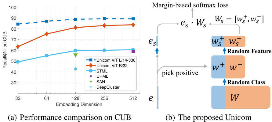
Figure 1: (a) Accuracy in Recall $@1$ versus embedding dimension on the CUB dataset. The proposed Unicom is only trained on the LAION 400M dataset without any manual annotation. (b) The proposed Unicom employs two random selections along the class dimension and the feature dimension to alleviate inter-class conflict and achieve compact representation, respectively.
图 1: (a) 在 CUB 数据集上 Recall $@1$ 准确率随嵌入维度的变化。所提出的 Unicom 仅在 LAION 400M 数据集上训练,未使用任何人工标注。(b) 所提出的 Unicom 沿类别维度和特征维度采用两种随机选择策略,分别用于缓解类间冲突和实现紧凑表示。
To handle the limitations of instance discrimination, cluster discrimination has been proposed for deep unsupervised learning through jointly learning image embeddings and cluster assignments. Learning representations with clusters will pull similar instances together, which is beneficial for capturing semantic structures in data. Deep Cluster (Caron et al., 2018) performs iterative clustering by k-means and classification by cross-entropy loss, while SeLa (Asano et al., 2020) proposes to solve an optimal transport problem for balanced assignment. However, both Deep Cluster and SeLa need labels to be assigned offline in a batch mode with representations of all instances. To reduce the cost of batch mode clustering, ODC (Zhan et al., 2020), SwAV (Caron et al., 2020), and CoKe (Qian et al., 2022) apply online clustering to avoid the multiple iterations over the entire dataset. Despite improved efficiency, the online clustering method still suffers from the collapsing problem (i.e., a dominant cluster includes instances from multiple classes or most of the instances).
为应对实例判别(instance discrimination)的局限性,研究者提出了通过联合学习图像嵌入和聚类分配的深度无监督学习方法——聚类判别(cluster discrimination)。基于聚类的表征学习能将相似实例聚合,有助于捕捉数据中的语义结构。Deep Cluster (Caron等人,2018)通过k均值迭代聚类并结合交叉熵损失进行分类,而SeLa (Asano等人,2020)则提出用最优传输问题求解平衡分配。但Deep Cluster和SeLa都需要基于所有实例的表征进行离线批量标签分配。为降低批量聚类成本,ODC (Zhan等人,2020)、SwAV (Caron等人,2020)和CoKe (Qian等人,2022)采用在线聚类来避免全数据集多次迭代。尽管效率提升,在线聚类仍存在坍缩问题(即主导聚类包含多类实例或大多数实例)。
In this paper, we aim at boosting the semantic embedding power of the CLIP model by introducing a novel cluster discrimination approach. We first conduct one step of off-line clustering by using the image and text features from a pre-trained CLIP model (Radford et al., 2021). Due to the limited discrimination power of the CLIP model, the pseudo clusters contain heavy inter-class conflict. Instead of optimizing the cluster assignment (Qian et al., 2022), we focus on how to robustly train a classifier on the automatically clustered large-scale data. More specifically, we explore two random selections on the prototype matrix $W\in R^{{d}\times k}$ when preparing the classification loss (as illustrated in Fig. 1(b)). The first one is with respect to the class dimension $(k)$ , and only part of negative prototypes are selected for inter-class comparisons, which helps alleviate inter-class conflict. The second one is with respect to the feature dimension $(d)$ , and only part of features are randomly selected to construct the classification loss, enhancing the representation power of each neuron and making feature representation compact for the efficient image retrieval task. Concurrent with our work, partial selection mechanisms along class and feature are separately proposed in (An et al., 2021; 2022) and (Xu et al., 2022) to accelerate model training and enhance locally distinguishable features. Both of their experiments are conducted on cleaned face recognition datasets. By contrast, we target at universal and compact representation learning from automatically clustered large-scale data. The main contributions of our paper are the following:
本文旨在通过引入一种新颖的聚类判别方法,提升CLIP模型(Radford等人,2021)的语义嵌入能力。我们首先利用预训练CLIP模型提取的图像和文本特征进行离线单步聚类。由于CLIP模型的判别能力有限,生成的伪聚类存在严重的类间冲突。与优化聚类分配(Qian等人,2022)不同,我们专注于如何在自动聚类的大规模数据上稳健训练分类器。具体而言,我们在构建分类损失时(如图1(b)所示),对原型矩阵$W\in R^{{d}\times k}$探索了两种随机选择机制:第一种沿类别维度$(k)$操作,仅选取部分负类原型进行类间比较,以缓解类间冲突;第二种沿特征维度$(d)$操作,随机选取部分特征构建分类损失,从而增强单个神经元的表征能力,并为高效图像检索任务生成紧凑特征表示。与我们同期的工作中,An等人(2021;2022)和Xu等人(2022)分别提出了沿类别和特征维度的部分选择机制以加速训练并增强局部可区分特征,但他们的实验均在清洗过的人脸识别数据集上进行。相比之下,我们的目标是实现自动聚类大规模数据的通用紧凑表征学习。本文主要贡献如下:
• We propose a novel cluster discrimination method for universal and compact representation learning. In the clustering step, we employ both image and text features from the pre-trained CLIP model. In the discrimination step, we explore two random selections along class and feature, which can potentially alleviate inter-class conflict and improve the feature compactness, respectively. • For both zero-shot learning tasks (e.g., linear probe and unsupervised image retrieval) and transfer learning tasks (e.g., ImageNet-1K classification and supervised image retrieval), the proposed random negative prototype selection for conflict-robust cluster discrimination can significantly boost the representation power compared to the instance discrimination based model (e.g., CLIP).
• 我们提出了一种新颖的聚类判别方法,用于通用且紧凑的表征学习。在聚类步骤中,我们同时采用预训练 CLIP 模型的图像和文本特征。在判别步骤中,我们探索了沿类别和特征两个维度的随机选择策略,分别用于缓解类间冲突和提升特征紧凑性。
• 在零样本学习任务(如线性探测和无监督图像检索)和迁移学习任务(如 ImageNet-1K 分类和有监督图像检索)中,所提出的基于随机负原型选择的冲突鲁棒聚类判别方法,相比基于实例判别的模型(如 CLIP),能显著提升表征能力。
2 RELATED WORK
2 相关工作
Visual Model Pre-training. Model pre-training for visual recognition can be categorized into three main groups: (1) supervised pre-training on datasets with manually annotated class labels (e.g., ImageNet-1K/-21K (Deng et al., 2009) and JFT-300M/-3B (Do sov it ski y et al., 2021; Zhai et al., 2022)), (2) weakly-supervised pre-training by using hashtag (Mahajan et al., 2018; Singh et al., 2022) or text descriptions (Radford et al., 2021; Jia et al., 2021), and (3) unsupervised pre-training (Chen et al., 2020; He et al., 2020; Caron et al., 2018). Since supervised pre-training relies on expensive manual annotations, we focus on annotation-free pre-training which has the advantages of being easily scaled to billions of training images and being able to learn universal feature representations for downstream tasks.
视觉模型预训练
视觉识别模型的预训练主要分为三类:(1) 在人工标注类别标签的数据集上进行监督式预训练 (如 ImageNet-1K/-21K (Deng et al., 2009) 和 JFT-300M/-3B (Dosovitskiy et al., 2021; Zhai et al., 2022)),(2) 通过话题标签 (Mahajan et al., 2018; Singh et al., 2022) 或文本描述 (Radford et al., 2021; Jia et al., 2021) 进行弱监督预训练,(3) 无监督预训练 (Chen et al., 2020; He et al., 2020; Caron et al., 2018)。由于监督式预训练依赖昂贵的人工标注,我们重点关注无需标注的预训练方法——其优势在于可轻松扩展至数十亿训练图像,并能学习适用于下游任务的通用特征表示。
Instance and Cluster Discrimination. Instance discrimination (Chen et al., 2020; He et al., 2020; Radford et al., 2021) is realized with a contrastive loss which targets at pulling closer samples from the same instance while pushing away samples from different instances. Despite the impressive performance, instance-wise contrastive learning can not capture the semantic information from the training data because it is trained to ignore the similarity between different instances. Cluster discrimination (Caron et al., 2018; Zhan et al., 2020; Li et al., 2020a) is processed with iterative steps: the clustering step to assign pseudo class labels for each sample, and then the classification step to map each sample to its assigned label. Since one cluster has more than one instance, learning representations with clusters will gather similar instances together, which can explore potential semantic structures in data. As a representative work, Deep Cluster (Caron et al., 2018) adopts a standard $\mathbf{k}$ -means for clustering, but it contains degenerate solutions. To this end, recent research work (Asano et al., 2020; Caron et al., 2020; Qian et al., 2022) focuses on improving the label assignment during clustering but employs a standard cross-entropy loss during discrimination. In this paper, we only employ one step of off-line clustering but design a robust classifier to achieve good feature representation when training on the automatically clustered large-scale data.
实例与聚类判别。实例判别 (Chen et al., 2020; He et al., 2020; Radford et al., 2021) 通过对比损失实现,其目标是拉近同一实例的样本,同时推开不同实例的样本。尽管性能出色,实例级对比学习无法捕捉训练数据中的语义信息,因为其训练目标要求忽略不同实例间的相似性。聚类判别 (Caron et al., 2018; Zhan et al., 2020; Li et al., 2020a) 采用迭代步骤:先通过聚类步骤为每个样本分配伪类标签,再通过分类步骤将样本映射到对应标签。由于一个聚类包含多个实例,基于聚类的表征学习会将相似实例聚集,从而挖掘数据中的潜在语义结构。代表性工作Deep Cluster (Caron et al., 2018) 采用标准 $\mathbf{k}$ -means聚类,但存在退化解问题。为此,近期研究 (Asano et al., 2020; Caron et al., 2020; Qian et al., 2022) 聚焦改进聚类时的标签分配,但在判别阶段仍使用标准交叉熵损失。本文仅采用单次离线聚类,但设计了鲁棒分类器以在自动聚类的大规模数据上训练时获得优质特征表征。
Image Retrieval. Image retrieval task typically relies on fine-tuning pre-trained visual models (Szegedy et al., 2015; He et al., 2016; Do sov it ski y et al., 2021) and can be divided into two learning categories: supervised and unsupervised metric learning. For supervised metric learning, pair-wise loss (Hadsell et al., 2006; Schroff et al., 2015; Sohn, 2016) and cross-entropy loss (Zhai & Wu, 2019; Deng et al., 2019; Sun et al., 2020; Qian et al., 2019) are extensively studied and recent bench-marking results (Musgrave et al., 2020) indicate that the margin-based softmax loss (e.g., ArcFace (Deng et al., 2019)) can achieve state-of-the-art performance. For unsupervised metric learning, pseudo labeling methods are employed to discover pseudo classes by applying k-means clustering (Kan et al., 2021; Li et al., 2020b), hierarchical clustering (Yan et al., 2021), random walk (Iscen et al., 2018), and class-equivalence relations (Kim et al., 2022) to unlabeled training data. In this paper, we focus on universal and compact feature embedding for both unsupervised and supervised image retrieval task.
图像检索。图像检索任务通常依赖于微调预训练的视觉模型 (Szegedy et al., 2015; He et al., 2016; Dosovitskiy et al., 2021),可分为监督和无监督度量学习两类。对于监督度量学习,成对损失 (Hadsell et al., 2006; Schroff et al., 2015; Sohn, 2016) 和交叉熵损失 (Zhai & Wu, 2019; Deng et al., 2019; Sun et al., 2020; Qian et al., 2019) 被广泛研究,近期基准测试结果 (Musgrave et al., 2020) 表明基于间隔的softmax损失(如ArcFace (Deng et al., 2019))能达到最先进性能。对于无监督度量学习,伪标签方法通过k均值聚类 (Kan et al., 2021; Li et al., 2020b)、层次聚类 (Yan et al., 2021)、随机游走 (Iscen et al., 2018) 和类等价关系 (Kim et al., 2022) 从未标注训练数据中发现伪类别。本文聚焦于无监督和监督图像检索任务的通用紧凑特征嵌入。
3 METHODOLOGY
3 方法论
3.1 PRELIMINARIES OF INSTANCE AND CLUSTER DISCRIMINATION
3.1 实例与聚类判别基础
Given a training set $X={x_{1},x_{2},...,x_{n}}$ including $n$ images, feature representation learning aims at learning a function $f$ that maps images $X$ to embeddings $E={e_{1},e_{2},...,e_{n}}$ with $e_{i}=f(x_{i})$ , such that embeddings can describe the similarities between different images. Instance discrimination achieves this objective by optimizing a contrastive loss function defined as:
给定一个包含 $n$ 张图像的训练集 $X={x_{1},x_{2},...,x_{n}}$,特征表示学习旨在学习一个函数 $f$,将图像 $X$ 映射到嵌入向量 $E={e_{1},e_{2},...,e_{n}}$(其中 $e_{i}=f(x_{i})$),使得嵌入向量能够描述不同图像之间的相似性。实例判别通过优化以下对比损失函数实现这一目标:
$$
\mathcal{L}{\mathrm{instance}}=-\sum_{i=1}^{n}\log\frac{\exp(e_{i}^{\prime T}e_{i})}{\sum_{j=0}^{m}\exp(e_{j}^{\prime T}e_{i})},
$$
$$
\mathcal{L}{\mathrm{instance}}=-\sum_{i=1}^{n}\log\frac{\exp(e_{i}^{\prime T}e_{i})}{\sum_{j=0}^{m}\exp(e_{j}^{\prime T}e_{i})},
$$
where $e_{i}$ and $e_{i}^{\prime}$ are positive embeddings of the instance $i$ , and $e_{j}^{\prime}$ consists of one positive embedding of $i$ and its $m$ negative embeddings from other instances.
其中 $e_{i}$ 和 $e_{i}^{\prime}$ 是实例 $i$ 的正向嵌入,$e_{j}^{\prime}$ 包含 $i$ 的一个正向嵌入及其来自其他实例的 $m$ 个负向嵌入。
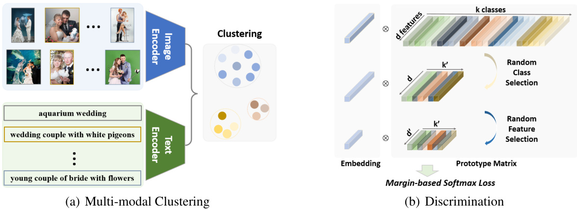
Figure 2: Illustration of the proposed method. (a) The multi-modal clustering includes one off-line step of k-means on features from image and text produced by a pre-trained CLIP model (Radford et al., 2021). (b) Using the assigned clusters as pseudo-labels, we propose a conflict-robust and representation-compact classification method through random class and feature selection along the two dimensions of the prototype matrix.
图 2: 所提方法示意图。(a) 多模态聚类包含一个离线步骤,即在预训练 CLIP 模型 (Radford et al., 2021) 生成的图像和文本特征上执行 k-means 聚类。(b) 通过将分配到的聚类作为伪标签,我们提出了一种冲突鲁棒且表征紧凑的分类方法,该方法沿着原型矩阵的两个维度进行随机类别和特征选择。
By contrast, cluster discrimination for representation learning consists of two main phases: clustering and discrimination. The clustering step assigns each instance a pseudo class label that will be subsequently used as supervision to train a classifier in the discrimination step. Following this, automatic clustering on the features $e_{i}=f(x_{i})$ is first performed to obtain $k$ clusters and the centroid $w_{i}$ is viewed as the prototype of $i$ -th cluster. Then, the training data ${x_{i}}{i=1}^{n}$ are partitioned into $k$ classes represented by prototypes $W={w_{i}}_{i=1}^{k}$ . With pseudo labels and centroids obtained from the clustering step, cluster discrimination can be implemented by optimizing a standard softmax classification loss as:
相比之下,表征学习的聚类判别包含两个主要阶段:聚类和判别。聚类步骤为每个实例分配一个伪类标签,随后该标签将作为监督信号用于判别步骤中的分类器训练。具体而言,首先对特征 $e_{i}=f(x_{i})$ 进行自动聚类得到 $k$ 个簇,并将质心 $w_{i}$ 视为第 $i$ 个簇的原型。随后,训练数据 ${x_{i}}{i=1}^{n}$ 被划分为由原型 $W={w_{i}}_{i=1}^{k}$ 表示的 $k$ 个类别。通过聚类步骤获得的伪标签和质心,可通过优化标准softmax分类损失来实现聚类判别:
$$
\mathcal{L}{\mathrm{cluster}}=-\sum_{i=1}^{n}\log\frac{\exp(w_{i}^{T}e_{i})}{\sum_{j=1}^{k}\exp(w_{j}^{T}e_{i})},
$$
$$
\mathcal{L}{\mathrm{cluster}}=-\sum_{i=1}^{n}\log\frac{\exp(w_{i}^{T}e_{i})}{\sum_{j=1}^{k}\exp(w_{j}^{T}e_{i})},
$$
where $e_{i}$ is the embedding of the image $x_{i}$ and $x_{i}$ belongs to the class represented by $w_{i}$ . By comparing Eq. 1 and Eq. 2, we can observe the difference that instance discrimination employs an augmented feature $e_{i}^{\prime}$ to calculate the similarities while cluster discrimination uses a prototype $w_{i}$ .
其中 $e_{i}$ 是图像 $x_{i}$ 的嵌入表示,且 $x_{i}$ 属于由 $w_{i}$ 代表的类别。通过对比式1和式2,我们可以观察到实例判别方法使用增强特征 $e_{i}^{\prime}$ 来计算相似度,而聚类判别方法则使用原型 $w_{i}$。
3.2 MULTIMODAL CLUSTERING
3.2 多模态聚类
In this paper, we focus on the standard clustering algorithm, $k$ -means, which takes a set of vectors as input and clusters them into $k$ distinct groups based on the nearest neighbor criterion. To seek a better representation, we combined the image and text features produced by the pre-trained CLIP model (Radford et al., 2021) due to their mutual complementary nature. The clustering step jointly learns a $d\times k$ centroid matrix $W$ and the cluster assignments $y_{i}$ of each image $x_{i}$ by solving the following problem:
本文重点研究标准聚类算法 $k$ -means,该算法以一组向量作为输入,根据最近邻准则将其聚类为 $k$ 个不同组别。为获得更好的表征,我们结合了预训练 CLIP 模型 (Radford et al., 2021) 生成的图像和文本特征,因其具有互补特性。聚类步骤通过求解以下问题,联合学习 $d\times k$ 质心矩阵 $W$ 及每张图像 $x_{i}$ 的聚类分配 $y_{i}$:
$$
\underset{W\in\mathbb{R}^{d\times k}}{\operatorname*{min}}\frac{1}{n}\sum_{i=1}^{n}\underset{y_{i}\in{0,1}^{k}}{\operatorname*{min}}\Vert\Phi(f(x_{i}),f^{\prime}(x_{i}^{\prime}))-W y_{i}\Vert_{2}^{2}\quad\mathrm{s.t.}\quad y_{i}^{\top}\mathbf{1_{k}}=\mathbf{1},
$$
$$
\underset{W\in\mathbb{R}^{d\times k}}{\operatorname*{min}}\frac{1}{n}\sum_{i=1}^{n}\underset{y_{i}\in{0,1}^{k}}{\operatorname*{min}}\Vert\Phi(f(x_{i}),f^{\prime}(x_{i}^{\prime}))-W y_{i}\Vert_{2}^{2}\quad\mathrm{s.t.}\quad y_{i}^{\top}\mathbf{1_{k}}=\mathbf{1},
$$
where $f(x_{i})$ is the image feature embedding by the image encoder $f$ and $f^{\prime}(x_{i}^{\prime})$ is the text feature embedding by the text encoder $f^{\prime}$ , $\Phi$ is a feature ensemble function, $W\in R^{d\times k}$ is the centroid matrix, $y_{i}$ in ${0,1}^{k}$ is a single label assignment constrained by $y_{i}^{\top}\mathbf{1_{k}}=\mathbf{1}$ , and ${\bf1_{k}}$ is 1-vector of size $k$ . In this work, we employ the simplest feature ensemble function, that is, averaging the image and text features, as the CLIP model provides an aligned visual-textual representation.
其中 $f(x_{i})$ 是图像编码器 $f$ 生成的图像特征嵌入,$f^{\prime}(x_{i}^{\prime})$ 是文本编码器 $f^{\prime}$ 生成的文本特征嵌入,$\Phi$ 是特征聚合函数,$W\in R^{d\times k}$ 是质心矩阵,${0,1}^{k}$ 中的 $y_{i}$ 是受 $y_{i}^{\top}\mathbf{1_{k}}=\mathbf{1}$ 约束的单标签分配,${\bf1_{k}}$ 是大小为 $k$ 的全1向量。本工作采用最简单的特征聚合函数(即对图像和文本特征取平均),因为 CLIP 模型提供了对齐的视觉-文本表示空间。
Considering that iterative clustering and discrimination are time-consuming, we only employ one step of off-line clustering in this work. Aided by the efficient feature quantization (Johnson et al., 2019), the large-scale LAION 400M dataset can be clustered within 10 minutes using the embedded image and text features. The only hyper-parameter we consider here is the cluster number $k$ . Even though the clustering step is straightforward, the automatically clustered large-scale dataset inevitably confronts inter-class conflict due to multi-label signals in one image and specific definition of class granularity (as illustrated in Fig. 3). For instance, the bird pair in Fig. 3(b) is clustered into wedding pair, which will be conflicted with another specific category of bird. In addition, the close-up capture of wedding flowers in Fig. 3(a) also exists in the class of wedding place, where flowers are the most popular decoration.
考虑到迭代式聚类和判别过程耗时较长,本研究仅采用单次离线聚类步骤。借助高效的特征量化技术 (Johnson et al., 2019),基于嵌入的图像与文本特征可在10分钟内完成LAION 400M大规模数据集的聚类。本文唯一涉及的超参数是聚类数量$k$。尽管聚类步骤简单直接,但自动聚类的大规模数据集仍会面临类间冲突问题,这源于单张图像的多标签信号以及类别粒度的特定定义(如图3所示)。例如,图3(b)中的鸟类配对样本被聚类至婚礼配对类别,这将与另一个特定的鸟类类别产生冲突。此外,图3(a)中婚礼花卉的特写镜头也存在于婚礼场地类别中,因为花卉是最常见的装饰元素。
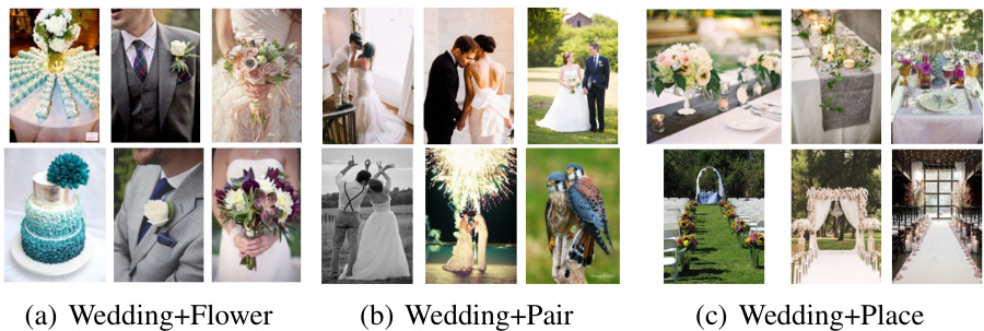
Figure 3: Inter-class conflict between the automatically-clustered classes. The class name is given based on the observation of images and texts. Inter-class conflict exists due to specific granularity definitions and multi-label signals in one image.
图 3: 自动聚类类别间的跨类冲突。类名基于对图像和文本的观察给出。由于特定粒度定义及单幅图像中的多标签信号,跨类冲突现象普遍存在。
3.3 CONFLICT-ROBUST AND REPRESENTATION-COMPACT DISCRIMINATION
3.3 冲突鲁棒且表征紧凑的判别方法
After the clustering step, we can employ a vanilla classification loss (e.g., softmax) to learn the feature representation. For the softmax loss given in Eq. 2, the derivatives to a class-wise prototype $w_{j}\in\mathbb{R}^{d}$ and a sample embedding feature $e_{i}\in\mathbb{R}^{d}$ are:
在聚类步骤之后,我们可以采用标准分类损失(如softmax)来学习特征表示。对于公式2给出的softmax损失,其对类别原型$w_{j}\in\mathbb{R}^{d}$和样本嵌入特征$e_{i}\in\mathbb{R}^{d}$的导数为:
$$
\frac{\partial\mathcal{L}}{\partial w_{j}}=\sum_{i=1}^{b}(p_{i j}-\mathbb{1}{y_{i}==\pm j})e_{i},~\frac{\partial\mathcal{L}}{\partial e_{i}}=\sum_{j=1}^{k}(p_{i j}-\mathbb{1}{y_{i}===j})w_{j},
$$
$$
\frac{\partial\mathcal{L}}{\partial w_{j}}=\sum_{i=1}^{b}(p_{i j}-\mathbb{1}{y_{i}==\pm j})e_{i},~\frac{\partial\mathcal{L}}{\partial e_{i}}=\sum_{j=1}^{k}(p_{i j}-\mathbb{1}{y_{i}===j})w_{j},
$$
where $b$ is the batch size, $k$ is the class number, and $p_{i j}\overset{j=1}{=}e^{w_{j}^{T}e_{i}}/\sum_{l=1}^{k}e^{w_{l}^{T}e_{i}}$ is the normalized probability of the sample embedding $e_{i}$ belonging to the prototype $w_{j}$ , $\bar{\mathbb{1}}(\bar{\cdot})$ is the indicator function which is 1 when the statement is true and 0 otherwise. In Eq. 4, the derivative of the prototype is a “weighted sum” over sample features from the mini-batch, and the derivative of the sample feature is a “weighted sum” over the prototypes of all classes. If conflicted classes exist, wrong gradient signals from these conflicted negative prototypes will affect the update of model parameters.
其中 $b$ 是批次大小,$k$ 是类别数,$p_{i j}\overset{j=1}{=}e^{w_{j}^{T}e_{i}}/\sum_{l=1}^{k}e^{w_{l}^{T}e_{i}}$ 表示样本嵌入 $e_{i}$ 属于原型 $w_{j}$ 的归一化概率,$\bar{\mathbb{1}}(\bar{\cdot})$ 是指示函数,当语句为真时取值为1,否则为0。在式4中,原型的导数是小批次样本特征的"加权和",而样本特征的导数是所有类别原型的"加权和"。若存在冲突类别,这些冲突负原型产生的错误梯度信号将影响模型参数的更新。
To this end, we propose a random negative prototype selection to efficiently construct a negative prototype subset from the entire negative prototypes. Therefore, the derivative to a sample embedding feature is:
为此,我们提出一种随机负原型选择方法,从全部负原型中高效构建负原型子集。因此,样本嵌入特征的导数为:
$$
\frac{\partial\mathcal{L}}{\partial e_{i}}=-((1-p^{+})w^{+}-\sum_{j\in\S,j\neq y_{i}}p_{j}^{-}w_{j}^{-}),
$$
$$
\frac{\partial\mathcal{L}}{\partial e_{i}}=-((1-p^{+})w^{+}-\sum_{j\in\S,j\neq y_{i}}p_{j}^{-}w_{j}^{-}),
$$
where $p^{+}$ and $w^{+}$ denote the probability and prototype of the positive class, $p_{j}^{-}$ and $w_{j}^{-}$ refer to negative probabilities and prototypes, $\mathbb{S}$ is a subset of all negative classes and one positive class, $|\mathbb{S}|=k*r_{1}$ , and $r_{1}\in[0,1]$ is the sampling ratio. Even though all class-wise prototypes are still maintained throughout the whole training process, only positive prototypes and a subset of negative prototypes are selected and updated in each iteration. Therefore, the inter-class conflict will be reduced as the possibility of sampling a conflict negative prototype is directly decreased by $r_{1}$ .
其中 $p^{+}$ 和 $w^{+}$ 表示正类的概率和原型,$p_{j}^{-}$ 和 $w_{j}^{-}$ 指代负类概率和原型,$\mathbb{S}$ 是所有负类与一个正类的子集,$|\mathbb{S}|=k*r_{1}$,且 $r_{1}\in[0,1]$ 为采样比例。尽管整个训练过程中仍保留所有类别的原型,但每次迭代仅选择并更新正类原型和部分负类原型。因此,通过 $r_{1}$ 直接降低冲突负类原型的采样概率,类间冲突将随之减少。
To achieve a compact representation for efficient image retrieval, previous methods (Babenko & Lempitsky, 2015; Tolias et al., 2016) adopt Principal Component Analysis (PCA) on an independent set for dimension reduction. To reduce the descriptor dimension to $d^{\prime}$ , only ei gen vectors corresponding to $d^{\prime}$ largest eigenvalues are retained. However, the representation produced by PCA is sub-optimal because it is a post-processing step detached from the target task. To this end, we propose a feature approximation strategy by randomly selecting subspace features to construct the classification loss:
为实现高效的图像检索紧凑表示,先前方法 (Babenko & Lempitsky, 2015; Tolias et al., 2016) 在独立数据集上采用主成分分析 (PCA) 进行降维。为将描述符维度降至 $d^{\prime}$ ,仅保留对应 $d^{\prime}$ 个最大特征值的特征向量。然而,PCA生成的表示存在次优性,因其作为后处理步骤与目标任务分离。为此,我们提出通过随机选择子空间特征构建分类损失的特征近似策略:
$$
\mathcal{L}{\mathrm{unicom}}=-\sum_{i=1}^{n}\log\frac{\exp((\Gamma_{t}\odot w_{i})^{T}(\Gamma_{t}\odot e_{i}))}{\sum_{j\in\mathbb{S}}\exp((\Gamma_{t}\odot w_{j})^{T}(\Gamma_{t}\odot e_{i}))},
$$
$$
\mathcal{L}{\mathrm{unicom}}=-\sum_{i=1}^{n}\log\frac{\exp((\Gamma_{t}\odot w_{i})^{T}(\Gamma_{t}\odot e_{i}))}{\sum_{j\in\mathbb{S}}\exp((\Gamma_{t}\odot w_{j})^{T}(\Gamma_{t}\odot e_{i}))},
$$
where $\Gamma_{t}\in{0,1}^{d}$ is a random binary vector at the iteration step of $t$ , the non-zero element ratio of $\Gamma_{t}$ is $r_{2}\in[0,1]$ , $\odot$ denotes element-wise product. Different from the well-known regular iz ation technique, Dropout (Srivastava et al., 2014), our random feature selection $\Gamma_{t}$ is same for all training samples within the mini-batch. $\Gamma_{t}$ is applied to both feature $e_{i}$ and prototypes $w_{j}$ , thus the dimension of derivatives in Eq. 4 decreases to $d^{\prime}$ . By contrast, Dropout is independently applied to each individual feature $e_{i}$ within the mini-batch by setting a specific ratio $r_{3}\in[0,1]$ of neurons to 0 and enlarging the rest neurons by $1/(1-r_{3})$ . The dimension of derivatives in Eq. 4 is still $d$ . Therefore, the sub-feature optimization in the proposed random feature selection can not be completed by directly calling the Dropout function. Since the binary vector varies at different iterations, different sub-features are trained and sub-gradients are calculated. This leads to a solution that each embedding neuron contains the similarity representation power.
其中 $\Gamma_{t}\in{0,1}^{d}$ 是第 $t$ 次迭代时的随机二值向量,$\Gamma_{t}$ 的非零元素比例为 $r_{2}\in[0,1]$,$\odot$ 表示逐元素乘积。与著名的正则化技术 Dropout (Srivastava et al., 2014) 不同,我们的随机特征选择 $\Gamma_{t}$ 对小批量内所有训练样本保持一致。$\Gamma_{t}$ 同时作用于特征 $e_{i}$ 和原型 $w_{j}$,因此式4中导数的维度降至 $d^{\prime}$。相比之下,Dropout 通过将神经元按比例 $r_{3}\in[0,1]$ 置零并将剩余神经元放大 $1/(1-r_{3})$ 倍,独立作用于小批量内每个特征 $e_{i}$,此时式4的导数维度仍为 $d$。因此,所提随机特征选择的子特征优化无法通过直接调用 Dropout 函数实现。由于二值向量在不同迭代时变化,不同子特征得到训练并计算次梯度,最终使得每个嵌入神经元都具备相似性表征能力。
The schematic of the proposed method is in Fig. 2(b). As shown, the prototype matrix $W$ is maintained in the memory at the dimension of $d\times k$ during the whole training process, but only part of the classes $(k^{\prime}=kr_{1})$ and features $(d^{\prime}=d*r_{2}$ ) are randomly selected to construct the softmax loss. The first random selection along the class dimension is for conflict-robust learning to achieve universal representation and the second random selection along the feature dimension is for feature compression required by efficient retrieval. Therefore, we name our method UNIversal and COMpact (UNICOM) representation learning.
所提方法的示意图如图 2(b) 所示。如图所示,原型矩阵 $W$ 在整个训练过程中以 $d\times k$ 的维度保存在内存中,但仅随机选择部分类别 $(k^{\prime}=kr_{1})$ 和特征 $(d^{\prime}=d*r_{2}$ ) 来构建 softmax 损失。沿类别维度的第一次随机选择是为了实现冲突鲁棒学习以获得通用表示,而沿特征维度的第二次随机选择则是为了满足高效检索所需的特征压缩。因此,我们将该方法命名为 UNIversal and COMpact (UNICOM) 表示学习。
4 EXPERIMENTS
4 实验
4.1 IMPLEMENTATION DETAILS
4.1 实现细节
Unless otherwise specified, all ViT models in our experiments follow the same architecture designs in CLIP, and are trained from scratch for 32 epochs on the automatically clustered LAION 400M dataset (Section 3.2) with cluster number $k=1M$ . During training, we randomly crop and horizontally flip each image to get the input image with $224\times224$ resolution. We set the random class sampling ratio $r_{1}$ as 0.1 in the pre-training step. The training is conducted on 128 NVIDIA V100 GPUs across 16 nodes. To save memory and scale up the batch size, mixed-precision and gradient checkpoint are used. We use AdamW (Loshchilov & Hutter, 2018) as the optimizer with an initial learning rate of 0.001, and a weight decay of 0.05. We employ margin-based softmax loss, ArcFace (Deng et al., 2019; 2020), for both pre-training and image retrieval tasks. The margin value is set to 0.3 and the feature scale is set to 64. For supervised retrieval, we follow the data-split settings of the baseline methods (Patel et al., 2022; Ermolov et al., 2022) to fine-tune models.
除非另有说明,本实验中所有ViT模型均遵循CLIP的相同架构设计,并在自动聚类的LAION 400M数据集(章节3.2)上从头开始训练32个周期,聚类数$k=1M$。训练期间,我们随机裁剪并水平翻转每张图像以获得$224\times224$分辨率的输入图像。预训练阶段将随机类别采样比例$r_{1}$设为0.1。训练在16个节点的128块NVIDIA V100 GPU上进行。为节省内存并扩大批次规模,采用了混合精度和梯度检查点技术。优化器使用AdamW (Loshchilov & Hutter, 2018),初始学习率为0.001,权重衰减为0.05。预训练和图像检索任务均采用基于间隔的softmax损失函数ArcFace (Deng et al., 2019; 2020),间隔值设为0.3,特征尺度设为64。对于有监督检索任务,我们遵循基线方法 (Patel et al., 2022; Ermolov et al., 2022) 的数据划分设置进行模型微调。
4.2 COMPARISONS ON FEATURE REPRESENTATION LEARNING
4.2 特征表示学习的比较
In this section, we first compare the performance of the proposed method and other baseline models (i.e., CLIP and OPEN-CLIP) on the linear probe and unsupervised image retrieval. Specifically, after the training on the automatically clustered 1M classes, we fix the backbones of our models. For the linear probe task, we learn an additional FC layer for classification on each test set. For unsupervised image retrieval, we directly use the embedding features for testing. Then, we fine-tune the pre-trained models for supervised image retrieval on each image retrieval dataset.
在本节中,我们首先比较了所提方法与其他基线模型(即 CLIP 和 OPEN-CLIP)在线性探测和无监督图像检索上的性能。具体而言,在自动聚类的 100 万类别上完成训练后,我们固定了模型的骨干网络。对于线性探测任务,我们在每个测试集上学习一个额外的全连接层进行分类。对于无监督图像检索,我们直接使用嵌入特征进行测试。随后,我们在每个图像检索数据集上对预训练模型进行监督式图像检索的微调。
Linear Probe. Following the same evaluation setting as CLIP (Radford et al., 2021), we freeze the pre-trained models on LAION 400M dataset and only fine-tune the last linear classification layer. We report the linear probing performance over 13 datasets in Tab. 1. The proposed conflict-robust cluster discrimination method significantly outperforms the CLIP and OPEN-CLIP (Ilharco et al., 2021) models. Notably, our ViT B/32, ViT B/16, and ViT L/14 models surpass counterparts of OPEN-CLIP by $3.6%$ , $2.7%$ and $1.4%$ on average with the same training data, indicating that the proposed cluster discrimination can enhance the representation power over instance discrimination.
线性探测 (Linear Probe)。遵循与 CLIP (Radford et al., 2021) 相同的评估设置,我们在 LAION 400M 数据集上冻结预训练模型,仅微调最后的线性分类层。如表 1 所示,我们报告了 13 个数据集的线性探测性能。提出的冲突鲁棒聚类判别方法显著优于 CLIP 和 OPEN-CLIP (Ilharco et al., 2021) 模型。值得注意的是,我们的 ViT B/32、ViT B/16 和 ViT L/14 模型在使用相同训练数据时,平均分别超越 OPEN-CLIP 对应模型 $3.6%$、$2.7%$ 和 $1.4%$,这表明所提出的聚类判别可以增强相对于实例判别的表示能力。
Unsupervised Image Retrieval. In Tab. 2, we compare the performance of unsupervised image retrieval by directly using the pre-trained models for feature embedding. The GLDv2 (Weyand et al., 2020) employs mean Average Precision $@100$ $\mathbf{\chi}{\mathrm{mAP}@100}^{\mathrm{}}$ ) as the evaluation metric, while other datasets use Recall $@1$ . Our ViT L/14 model achieves $69.9%$ average result across 7 image retrieval datasets, surpassing the OPEN-CLIP counterpart by $7.5%$ and even outperforming the larger OPEN-CLIP model ViT H/14 by $5.4%$ . The reason behind this significant improvement is that the proposed cluster discrimination can capture the semantic structure in data, which is crucial for the image retrieval task. In Fig. 1(a), we compare our method with the state-of-the-art unsupervised image retrieval approach, STML (Kim et al., 2022), under different dimension constraints on the CUB dataset. We set the random feature selection ratio $r_{2}$ as 0.5 for one additional training epoch on the LAION 400M dataset. Then, we select the first 256-D, 128-D, 64-D, and 32-D features for testing.
无监督图像检索。在表 2 中,我们比较了直接使用预训练模型进行特征嵌入的无监督图像检索性能。GLDv2 (Weyand et al., 2020) 采用平均精度均值 $@100$ ($\mathbf{\chi}{\mathrm{mAP}@100}^{\mathrm{}}$) 作为评估指标,其他数据集则使用召回率 $@1$。我们的 ViT L/14 模型在 7 个图像检索数据集上取得了 $69.9%$ 的平均结果,比 OPEN-CLIP 对应模型高出 $7.5%$,甚至优于更大的 OPEN-CLIP 模型 ViT H/14 达 $5.4%$。这一显著提升的原因是所提出的聚类判别方法能够捕捉数据中的语义结构,这对图像检索任务至关重要。在图 1(a) 中,我们在 CUB 数据集上比较了我们的方法与最先进的无监督图像检索方法 STML (Kim et al., 2022) 在不同维度约束下的表现。我们在 LAION 400M 数据集上额外训练一个 epoch 时,将随机特征选择比例 $r_{2}$ 设为 0.5。然后,我们选取前 256 维、128 维、64 维和 32 维特征进行测试。
Table 1: Top-1 accuracy $(%)$ of linear probe on 13 image classification datasets. The proposed cluster discrimination significantly outperforms OPEN-CLIP (Ilharco et al., 2021) on average by using the same training data (i.e., LAION 400M). “CLIP-R” denotes testing the public CLIP-ViT models in our code base. $\ '-336'$ refers to one additional epoch of pre-training at a higher $336\times336$ resolution to boost performance.
表 1: 13个图像分类数据集上线性探针的Top-1准确率$(%)$。使用相同训练数据(即LAION 400M)时,所提出的聚类判别方法平均显著优于OPEN-CLIP (Ilharco et al., 2021)。"CLIP-R"表示在我们的代码库中测试公开的CLIP-ViT模型。$\ '-336'$指在更高$336\times336$分辨率下增加一个预训练周期以提升性能。
| 10 FAR CIFA | 0 CIFAR1 | Caltechl C | C | Flowers | d101 Foodl | Birdsnap | SUN397 | TD | Aircraft | Pets | S Euros | ImageNet | Average | ||
|---|---|---|---|---|---|---|---|---|---|---|---|---|---|---|---|
| ViTB/32 | 95.1 | 80.5 | 93.0 | 81.8 | 96.9 | 88.8 | 58.5 | 76.6 | 76.5 | 52.0 | 90.0 | 97.0 | 76.1 | 81.8 | |
| ViT B/16 | 96.2 | 83.1 | 94.7 | 86.7 | 98.1 | 92.8 | 67.8 | 78.4 | 79.2 | 59.5 | 93.1 | 97.1 | 80.2 | 85.1 | |
| ViT L/14 | 98.0 | 87.5 | 96.5 | 90.9 | 99.2 | 95.2 | 77.0 | 81.8 | 82.1 | 69.4 | 95.1 | 98.2 | 83.9 | 88.8 | |
| ViT L/14-336 | 97.9 | 87.4 | 96.0 | 91.5 | 99.2 | 95.9 | 79.9 | 82.2 | 83.0 | 71.6 | 95.1 | 98.1 | 85.4 | 89.5 | |
| R ViTB/32 | 96.0 | 82.5 | 94.1 | 86.0 | 97.8 | 92.7 | 61.1 | 79.1 | 78.4 | 58.9 | 93.0 | 95.3 | 75.3 | 83.9 | |
| ViTB/16 | 96.0 | 82.5 | 94.1 | 86.0 | 97.8 | 92.7 | 69.5 | 79.1 | 78.4 | 58.9 | 93.0 | 95.3 | 79.6 | 84.8 | |
| ViT L/14 | 98.1 | 87.2 | 96.0 | 90.7 | 99.2 | 95.3 | 77.8 | 81.5 | 80.9 | 68.0 | 94.9 | 96.7 | 84.1 | 88.5 | |
| P ViT L/14-336 | 97.8 | 87.1 | 96.3 | 91.4 | 99.2 | 95.9 | 80.9 | 82.2 | 82.4 | 71.2 | 95.1 | 96.8 | 84.9 | 89.3 | |
| ViTB/32 | 95.3 | 82.2 | 93.3 | 87.5 | 96.5 | 86.2 | 61.4 | 75.3 | 78.8 | 52.4 | 88.0 | 96.5 | 73.8 | 82.1 | |
| ViTB/16 | 96.4 | 84.0 | 94.1 | 91.8 | 98.1 | 90.7 | 71.2 | 78.7 | 81.6 | 59.3 | 90.0 | 96.2 | 78.5 | 85.4 | |
| OPE ViT L/14 | 97.9 | 87.9 | 95.5 | 93.6 | 98.8 | 93.3 | 78.0 | 81.0 | 83.0 | 64.4 | 93.3 | 97.1 | 81.5 | 88.1 | |
| 98.5 | 85.8 | 70.2 | 74.6 | 78.0 | 70.7 | ||||||||||
| sIn ViTB/32 | 96.8 | 86.6 | 94.6 | 93.3 | 93.1 | 96.8 | 75.0 | 85.7 | |||||||
| ViTB/16 | 97.3 | 87.7 | 95.1 | 94.3 | 98.9 | 91.2 | 79.3 | 77.1 | 81.2 | 73.4 | 93.9 | 97.0 | 79.1 | 88.1 | |
| ViT L/14 | 98.5 | 90.8 | 95.7 | 94.6 | 99.3 | 93.4 | 82.4 | 80.0 | 82.2 | 74.5 | 94.2 | 96.7 | 81.8 | 89.5 | |
| ViT L/14-336 | 98.5 | 90.7 | 95.7 | 95.1 | 99.4 | 94.3 | 85.1 | 79.7 | 82.0 | 78.1 | 94.5 | 97.2 | 82.7 | 90.2 |
Table 2: Performance of unsupervised image retrieval on 7 image retrieval datasets. The proposed conflict-robust cluster discrimination significantly outperforms OPEN-CLIP on average by using the same training data.
表 2: 7个图像检索数据集上的无监督图像检索性能。所提出的冲突鲁棒聚类判别方法在使用相同训练数据的情况下,平均性能显著优于OPEN-CLIP。
| CUB | Cars | SOP | In-Shop | INaturalist | VehicleID | GLDv2 | Average | |||||
|---|---|---|---|---|---|---|---|---|---|---|---|---|
| Small | Medium | Large | Private | Public | ||||||||
| B/32 B/16 L/14 | 56.7 66.1 | 79.0 85.2 | 60.5 63.2 | 45.4 56.1 | 53.0 63.1 | 54.8 55.1 | 52.2 50.9 | 44.6 43.8 | 7.5 8.4 | 7.5 10.6 | 46.1 | |
| 76.0 | 90.3 | 65.6 | 50.3 | |||||||||
| L/14-336 | 90.9 | 67.8 | 62.9 | 72.9 | 62.4 | 58.9 | 51.8 | 12.1 | 13.6 | 56.7 | ||
| 77.3 | 66.3 | 76.8 | 64.1 | 60.3 | 53.8 | 17.0 | 15.6 | 59.0 | ||||
| OPI | B/32 B/16 L/14 | 62.3 71.4 | 89.2 65.9 | 64.6 | 54.9 | 71.0 | 67.1 | 59.9 | 9.17 | 8.4 | 55.2 | |
| 79.4 | 92.9 94.9 | 68.7 70.6 | 74.2 | 64.1 | 73.3 | 70.1 | 63.7 | 12.1 | 11.0 | 60.2 | ||
| H/14 | 83.1 | 77.1 | 71.0 | 72.0 | 69.1 | 62.0 | 14.5 | 13.8 | 62.4 | |||
| 95.7 | 72.7 | 78.8 | 77.0 | 72.7 | 69.7 | 61.9 | 17.7 | 15.3 | 64.5 | |||
| s.Ino | B/32 B/16 | 83.7 | 95.9 | 70.0 | 72.8 | 64.6 | 74.9 | 72.0 | 65.4 | 15.1 | 13.3 | 62.8 |
| 86.5 | 96.8 | 70.4 | 74.6 | 73.6 | 74.5 | 70.6 | 58.7 | 18.7 | 17.2 | 64.2 | ||
| L/14 | 88.5 | 96.9 | 72.7 | 83.6 | 77.1 | 83.7 | 80.2 | 74.6 | 21.1 | 20.1 | 69.9 | |
| L/14-336 | 89.2 | 97.3 | 74.5 | 86.7 | 81.0 | 84.1 | 81.4 | 75.6 | 23.2 | 22.0 | 71.5 |
STML employs an ImageNet-1K pre-trained GoogleNet (Szegedy et al., 2015) and then explores unsupervised training on the CUB dataset. Even though our ViT-based model is only trained on the automatically clustered LAION 400M dataset without any further training on the image retrieval dataset, our method outperforms STML (Kim et al., 2022) by a large margin across different test dimensions, indicating the superiority of the proposed random feature selection for compact feature representation learning.
STML采用了在ImageNet-1K上预训练的GoogleNet (Szegedy等人, 2015) ,然后在CUB数据集上探索无监督训练。尽管我们基于ViT的模型仅在自动聚类的LAION 400M数据集上训练,未经过任何图像检索数据集的额外训练,但我们的方法在不同测试维度上大幅优于STML (Kim等人, 2022) ,这表明所提出的随机特征选择方法在紧凑特征表示学习方面具有优越性。
Fine-tune for ImageNet-1K Classification. In Tab. 3, we compare our method with state-of-the-art supervised and weakly supervised pre-training (Do sov it ski y et al., 2021; Zhai et al., 2022; Singh et al., 2022) in transfer-learning experiments on ImageNet-1k. Our models consistently outperform OPENCLIP models in the Top-1 accuracy, showing the superiority of the proposed cluster discrimination. For ViT B/16, our pre-training achieves $85.9%$ , surpassing both the supervised pre-training on IN-21K $(84.0%)$ and the weakly supervised pre-training on IG 3.6B $(85.3%)$ . In addition, our ViT L/14 obtains $88.3%$ , outperforming ViT L/16 pre-trained on JFT 300M $(87.8%)$ and ViT L/16 pre-trained on IG 3.6B $(88.1%)$ . The overall results in ImageNet-1K classification task show that our models are very competitive as they can achieve better or comparable accuracy even though the training data used by the competitors are much larger (e.g., JFT 3B and IG 3.6B).
ImageNet-1K分类微调。在表3中,我们将本方法与ImageNet-1k迁移学习实验中最先进的监督和弱监督预训练方法(Do sov it ski y et al., 2021; Zhai et al., 2022; Singh et al., 2022)进行对比。我们的模型在Top-1准确率上始终优于OPENCLIP模型,证明了所提出的聚类判别方法的优越性。对于ViT B/16,我们的预训练达到了$85.9%$,超过了IN-21K上的监督预训练$(84.0%)$和IG 3.6B上的弱监督预训练$(85.3%)$。此外,我们的ViT L/14获得了$88.3%$的准确率,优于JFT 300M上预训练的ViT L/16$(87.8%)$和IG 3.6B上预训练的ViT L/16$(88.1%)$。ImageNet-1K分类任务的总体结果表明,我们的模型极具竞争力,即使在竞争对手使用的训练数据量更大(如JFT 3B和IG 3.6B)的情况下,仍能取得更好或相当的准确率。
Table 3: Transfer-learning accuracy of models pre-trained on the specified dataset followed by fine-tuning and testing on ImageNet.
表 3: 模型在指定数据集上预训练后经微调并在 ImageNet 上测试的迁移学习准确率。
| 模型 | 预训练数据集 | 预训练分辨率 | 微调分辨率 | IN-1K Top-1 准确率 | FLOPs (B) |
|---|---|---|---|---|---|
| 监督式预训练 | |||||
| ViT L/32 (Dosovitskiy et al., 2021) | IN-21k | 224 | 384 | 81.3 | 54.4 |
| ViT B/16 (Dosovitskiy et al., 2021) | IN-21k | 224 | 384 | 84.0 | 55.6 |
| ViT L/16 (Dosovitskiy et al., 2021) | IN-21k | 224 | 384 | 85.2 | 191.5 |
| ViT L/16 (Dosovitskiy et al., 2021) | JFT 300M | 224 | 512 | 87.8 | 362.9 |
| ViT L/16 (Zhai et al., 2022) | JFT3B | 224 | 384 | 88.5 | 191.5 |
| 弱监督式预训练 | |||||
| ViT B/16 (Singh et al., 2022) | IG 3.6B | 224 | 384 | 85.3 | 55.6 |
| ViT L/16 (Singh et al., 2022) | IG 3.6B | 224 | 512 | 88.1 | 362.9 |
| ViT B/32 OPEN-CLIP | LAION 400M | 224 | 384 | 83.0 | 15.5 |
| ViT B/16 OPEN-CLIP | LAION 400M | 224 | 384 | 85.4 | 55.6 |
| ViT L/14 OPEN-CLIP | LAION 400M | 224 | 518 | 87.7 | 507.8 |
| ViT B/32 Ours | LAION 400M | 224 | 384 | 83.6 | 15.5 |
| ViT B/16 Ours | LAION 400M | 224 | 384 | 85.9 | 55.6 |
| ViT L/14 Ours | LAION 400M | 224 | 518 | 88.3 | 507.8 |
Table 4: Performance of supervised image retrieval on 7 image retrieval datasets.
表 4: 7个图像检索数据集上的监督式图像检索性能。
| ViT-B/32 | ViT-B/16 | ViT-L/14 | ViT-L/14-336 | PreviousSOTA | |
|---|---|---|---|---|---|
| CUB | 85.8 | 88.8 | 89.7 | 90.1 | 85.6 viT-s/16 (Ermolov et al., 2022) |
| Cars | 97.3 | 97.7 | 97.9 | 98.2 | 94.8 sE-ResNet-50 (Jun et al., 2019) |
| SOP | 87.1 | 88.8 | 89.9 | 91.2 | 88.0 viT-B/16 (Patel et al., 2022) |
| In-Shop | 94.8 | 95.5 | 96.0 | 96.7 | 92.7 viT-s/16 (Ermolov et al., 2022) |
| INaturalist | 72.8 | 82.5 | 85.4 | 88.9 | 83.9 viT-B/16 (Patel et al., 2022) |
| VehicleID-Small | 95.4 | 96.4 | 96.5 | 97.0 | 96.2 viT-B/16 (Patel et al., 2022) |
| VehicleID-Medium | 94.1 | 95.1 | 95.7 | 96.1 | 95.2 viT-B/16 (Patel et al., 2022) |
| VehicleID-Large | 93.6 | 95.0 | 95.4 | 96.0 | 94.7 viT-B/16 (Patel et al., 2022) |
| GLDv2-Private | 32.6 | 35.7 | 36.1 | 36.4 | 32.5 ResNet101 (Lee et al., 2022) |
| GLDv2-Public | 29.7 | 32.4 | 33.0 | 33.1 | 24.6 ResNet50 (Tan et al., 2021) |
Fine-tune for Supervised Image Retrieval. In Tab. 4, we compare the proposed approach with the latest image retrieval methods (Patel et al., 2022; Ermolov et al., 2022) trained with vision transformer. During fine-tuning of our models, the random negative class selection ratio $r_{1}$ is set to 1.0 as the training data is clean. Under different computing regimes, the proposed method consistently surpasses $\mathtt{R A@K}$ (Patel et al., 2022) on the SOP, i Naturalist, and VehicleID datasets and outperforms Hyp-ViT (Ermolov et al., 2022) on the CUB and In-shop datasets.
监督式图像检索的微调。在表4中,我们将所提出的方法与基于视觉Transformer (vision transformer) 训练的最新图像检索方法 (Patel et al., 2022; Ermolov et al., 2022) 进行了比较。在模型微调过程中,由于训练数据干净,随机负类选择比例 $r_{1}$ 设为1.0。在不同计算规模下,所提方法在SOP、iNaturalist和VehicleID数据集上持续超越 $\mathtt{R A@K}$ (Patel et al., 2022),并在CUB和In-shop数据集上优于Hyp-ViT (Ermolov et al., 2022)。
4.3 ABLATION STUDY
4.3 消融实验
Encoder for Clustering. In Tab. 5, we compare the results of linear probe and unsupervised image retrieval under image-based clustering and text-based clustering by using the pre-trained CLIP and OPEN-CLIP models. As we can see, the text encoder is more powerful than the image encoder, and image and text signals are complementary as the joint clustering significantly outperforms each individual. By referring to Tab. 1 and Tab. 2, the OPEN-CLIP ViT B/32 model achieves $82.1%$ and $55.2%$ average results on the linear probe and unsupervised image retrieval tasks, while the proposed cluster discrimination method $\zeta_{1}=0.1$ ) significantly boosts the performance to $84.1%$ and $61.1%$ by using the OPEN-CLIP image and text models for clustering. By using the CLIP image and text models for clustering, the performance can further increase to $\bar{85.7}%$ and $62.8%$ on the linear probe and unsupervised image retrieval tasks. Therefore, we choose the CLIP models for clustering.
聚类编码器。在表5中,我们比较了使用预训练CLIP和OPEN-CLIP模型时,基于图像聚类和基于文本聚类的线性探测与无监督图像检索结果。可以看出,文本编码器比图像编码器更强大,且图像与文本信号具有互补性——联合聚类的表现显著优于单独使用任一模态。参考表1和表2,OPEN-CLIP ViT B/32模型在线性探测和无监督图像检索任务上分别取得82.1%和55.2%的平均结果,而采用OPEN-CLIP图像与文本模型进行聚类时,所提出的聚类判别方法(ζ₁=0.1)将性能显著提升至84.1%和61.1%。若改用CLIP图像与文本模型进行聚类,线性探测和无监督图像检索任务的性能可进一步提升至85.7%和62.8%。因此我们最终选择CLIP模型进行聚类。
Cluster Number. In Tab. 5, we also compare the performance under different cluster numbers, i.e., 100K, 1M, and 10M, by using the CLIP image and text models. As can be seen, the best results can be achieved when the cluster number is set as 1 million, with the average image number per class being around 400. The cluster number needs to be balanced between the intra-class noises and inter-class noises. Too small cluster numbers will incur heavy intra-class noise, which dramatically decreases the performance of the pre-trained classification model. Besides, too many clusters will increase the computation and storage burden on the FC layer. Most important, the over-decomposition will increase the inter-class noise ratio and undermine the disc rim i native power of the pre-trained model.
聚类数量。在表5中,我们还比较了使用CLIP图像和文本模型时不同聚类数量(即10万、100万和1000万)下的性能表现。可以看出,当聚类数量设置为100万时(每类平均图像数约为400)能获得最佳结果。聚类数量需要在类内噪声与类间噪声之间取得平衡:过少的聚类数量会导致严重的类内噪声,这会显著降低预训练分类模型的性能;过多的聚类则会增加全连接层的计算和存储负担。最重要的是,过度分解会提高类间噪声比例,削弱预训练模型的判别能力。
Table 5: Ablation study on multi-modal clustering. ViT B/32 is used here for model training on the LAION 400M dataset, which is automatically clustered by different pre-trained models. We report the average performance of linear probe and unsupervised image retrieval.
表 5: 多模态聚类消融研究。此处使用 ViT B/32 在 LAION 400M 数据集上进行模型训练,该数据集由不同预训练模型自动聚类。我们报告了线性探测和无监督图像检索的平均性能。
| Tasks | Image | CLIP Text | Joint | OPEN-CLIP | Cluster Number by CLIP | ||||
|---|---|---|---|---|---|---|---|---|---|
| Image | Text | Joint | 100K | 1M | 10M | ||||
| Linear Probe | 84.4 | 85.3 | 85.7 | 83.9 | 84.0 | 84.1 | 75.9 | 85.7 | 83.6 |
| Unsup. Retr. | 61.8 | 62.3 | 62.8 | 58.9 | 60.1 | 61.1 | 53.2 | 62.8 | 60.7 |
Table 6: Ablation study on random negative class selection and random feature selection. ViT-B/32 is used here and we report the average performance of linear probe and unsupervised image retrieval.
表 6: 随机负类选择与随机特征选择的消融研究。此处使用 ViT-B/32 并报告线性探测和无监督图像检索的平均性能。
| 任务 | 随机类别比例 (r1) 0.05 | 0.1 | 0.3 | 随机特征比例 (r2) 1.0 | 0.5 | 0.25 | Dropout比例 (r3) 0.25 | 0.5 |
|---|---|---|---|---|---|---|---|---|
| LinearProbe | 85.1 | 85.7 | 84.9 | 1.0 | 77.9 | 85.7 | 85.5 | 84.2 |
| Unsup. Retr. | 62.3 | 62.8 | 62.1 | 55.9 | 62.8 | 62.7 | 62.0 | 62.5 |
| Unsup. Retr. 256 | 61.4 | 61.8 | 61.0 | 60.7 |
Random Class Selection. In Tab. 6, we train ViT B/32 models under different inter-class sampling ratios. The basic margin-based softmax loss $\zeta_{1}=1.0$ ) only achieves $77.9%$ on the linear probe task as it can hardly adapt to the heavy inter-class conflict in the automatically clustered dataset. When the sampling ratio is decreased from 1.0 to 0.3 and 0.1, our method exhibits consistently better performance than the baseline, indicating random inter-class sampling is beneficial for the model’s robustness. When $r_{1}$ is set to 0.05, there is a slight performance drop because the inter-class interaction is insufficient during training. Therefore, we choose the random negative class selection ratio as 0.1, obtaining $85.7%$ and $62.8%$ on the linear probe and unsupervised image retrieval tasks.
随机类别选择。在表6中,我们在不同类别间采样比例下训练ViT B/32模型。基于边界的基本softmax损失($\zeta_{1}=1.0$)在线性探测任务中仅达到$77.9%$,因为它难以适应自动聚类数据集中严重的类别间冲突。当采样比例从1.0降至0.3和0.1时,我们的方法始终表现出优于基线的性能,表明随机类别间采样有助于提升模型鲁棒性。当$r_{1}$设为0.05时,由于训练期间类别间交互不足,性能出现小幅下降。因此,我们选择0.1作为随机负类采样比例,在线性探测和无监督图像检索任务中分别获得$85.7%$和$62.8%$的结果。
Random Feature Selection. In Tab. 6, we compare the performance of the proposed Unicom under different random feature selection ratios $(r_{2})$ on the task of dimension-constrained unsupervised image retrieval. Here, we also include Dropout at different drop ratios $(r_{3})$ for comparison. From the results, we can have the following observations: (1) both random feature selection and Dropout can not improve linear probe and unsupervised image retrieval at a full dimension of 512 as the LAION 400M dataset is large enough and regular iz ation is not necessary for the final classification layer, (2) there is slight performance drop when the random feature selection ratio is decreasing, and (3) the proposed random feature selection $\mathit{\Omega}{\mathit{r}_{2}}=0.5$ can improve $0.4%$ for 256-D unsupervised image retrieval, while Dropout can not improve dimension-constrained unsupervised image retrieval. Even though Dropout enforces partial features for classification, the global random iz ation within the mini-batch makes the optimization involve all feature dimensions. By contrast, the proposed random feature selection is fixed within the mini-batch thus it can benefit from optimization in a sub-feature space.
随机特征选择。在表6中,我们比较了所提出的Unicom在不同随机特征选择比例$(r_{2})$下在维度受限无监督图像检索任务中的性能。这里,我们还加入了不同丢弃比例$(r_{3})$的Dropout进行比较。从结果中可以得到以下观察:(1) 随机特征选择和Dropout都无法在512维全维度上提升线性探测和无监督图像检索性能,因为LAION 400M数据集足够大且最终分类层不需要正则化,(2) 当随机特征选择比例降低时性能略有下降,(3) 所提出的随机特征选择$\mathit{\Omega}{\mathit{r}_{2}}=0.5$可以将256维无监督图像检索性能提升$0.4%$,而Dropout无法提升维度受限的无监督图像检索性能。尽管Dropout强制使用部分特征进行分类,但小批量内的全局随机化使得优化涉及所有特征维度。相比之下,所提出的随机特征选择在小批量内是固定的,因此可以从子特征空间的优化中受益。
5 CONCLUSIONS
5 结论
This paper introduces Unicom, a simple yet effective framework for universal and compact feature embedding. Given the automatically clustered large-scale data, we employ one random negative class selection to improve the robustness under the heavy inter-class conflict and another random feature selection to improve the compactness of the feature representation. For both unsupervised and supervised image retrieval on different datasets, the proposed Unicom achieves state-of-the-art performance, confirming that cluster discrimination is beneficial to explore the semantic structure within the large-scale training data.
本文介绍了Unicom,一个简单而高效的通用紧凑特征嵌入框架。基于自动聚类的大规模数据,我们采用随机负类选择策略增强类间冲突下的鲁棒性,并通过随机特征选择提升特征表示的紧凑性。在不同数据集的无监督和有监督图像检索任务中,Unicom均实现了最先进的性能,证实了聚类判别方法有助于挖掘大规模训练数据中的语义结构。
A.4 COMPARISONS ON COCO DETECTION AND SEGMENTATION
A.4 COCO检测与分割对比
Following the experiment setting in (Li et al., 2022), we use Mask R-CNN (He et al., 2017) for bounding-box object detection and instance segmentation. We fine-tune models on the COCO (Lin et al., 2014) train2017 split and evaluate on the val2017 split. In Tab. 9, our method outperforms both OPEN-CLIP and supervised pre-training in all metrics, demonstrating the effectiveness of the proposed cluster discrimination.
按照 (Li et al., 2022) 的实验设置,我们采用 Mask R-CNN (He et al., 2017) 进行边界框目标检测和实例分割。模型在 COCO (Lin et al., 2014) 的 train2017 划分上进行微调,并在 val2017 划分上评估。如 表 9 所示,我们的方法在所有指标上均优于 OPEN-CLIP 和监督式预训练,证明了所提出的聚类判别方法的有效性。
A.5 LINEAR PROBE DATASETS
A.5 线性探测数据集
We use 13 image classification datasets to prove the effectiveness of our method. These datasets include CIFAR10(Krizhevsky & Hinton, 2009), CIFAR100(Krizhevsky & Hinton, 2009), Caltech101(Fei-Fei et al., 2004), Stanford Cars(Krause et al., 2013a), Oxford Flowers(Nilsback & Zisserman, 2008), Food-101(Bossard et al., 2014), Birdsnap(Berg et al., 2014), SUN397(Xiao et al., 2010), Describable Textures(Cimpoi et al., 2014), FGVC Aircraft(Maji et al., 2013), Oxford-IIIT Pets(Parkhi et al., 2012), EuroSAT(Helber et al., 2019), ImageNet-1k(Russ a kov sky et al., 2015). Details on each dataset and the corresponding evaluation metrics are provided in Tab. 10.
我们使用13个图像分类数据集来验证方法的有效性。这些数据集包括CIFAR10(Krizhevsky & Hinton, 2009)、CIFAR100(Krizhevsky & Hinton, 2009)、Caltech101(Fei-Fei et al., 2004)、Stanford Cars(Krause et al., 2013a)、Oxford Flowers(Nilsback & Zisserman, 2008)、Food-101(Bossard et al., 2014)、Birdsnap(Berg et al., 2014)、SUN397(Xiao et al., 2010)、Describable Textures(Cimpoi et al., 2014)、FGVC Aircraft(Maji et al., 2013)、Oxford-IIIT Pets(Parkhi et al., 2012)、EuroSAT(Helber et al., 2019)和ImageNet-1k(Russakovsky et al., 2015)。各数据集详情及对应评估指标见表10。
A.6 IMAGE RETRIEVAL DATASETS
A.6 图像检索数据集
The training and evaluation of image retrieval experiments on seven widely used datasets, namely CUB-200-2011(CUB) (Welinder et al., 2010), Stanford Cars(Cars196) (Krause et al., 2013b), Stanford Online Products(SOP) (Oh Song et al., 2016), In-shop Clothes Retrieval(In-Shop) (Liu et al., 2016b), i Naturalist (Van Horn et al., 2018), VehicleID (Liu et al., 2016a), and Google Landmarks dataset (GLDv2) (Weyand et al., 2020). The number of examples and classes can be found in Tab. 11.
在七个广泛使用的数据集上进行了图像检索实验的训练和评估,分别是CUB-200-2011(CUB) (Welinder et al., 2010)、Stanford Cars(Cars196) (Krause et al., 2013b)、Stanford Online Products(SOP) (Oh Song et al., 2016)、In-shop Clothes Retrieval(In-Shop) (Liu et al., 2016b)、i Naturalist (Van Horn et al., 2018)、VehicleID (Liu et al., 2016a)和Google Landmarks dataset(GLDv2) (Weyand et al., 2020)。样本数量和类别数见表11。
Table 10: List of linear probe datasets with the data distribution and evaluation metrics.
表 10: 线性探测数据集列表(含数据分布与评估指标)
| 数据集 | 类别数 | 训练集规模 | 测试集规模 | 评估指标 |
|---|---|---|---|---|
| CIFAR-10 | 10 | 50,000 | 10,000 | 准确率 |
| CIFAR-100 | 100 | 50,000 | 10,000 | 准确率 |
| Caltech-101 | 102 | 3,060 | 6,085 | 类平均准确率 |
| Stanford Cars | 196 | 8,144 | 8,041 | 准确率 |
| OxfordFlowers | 102 | 2,040 | 6,149 | 类平均准确率 |
| Food-101 | 102 | 75,750 | 25,250 | 准确率 |
| Birdsnap | 500 | 42,283 | 2,149 | 准确率 |
| SUN397 | 397 | 19,850 | 19,850 | 准确率 |
| DescribableTextures | 47 | 3,760 | 1,880 | 准确率 |
| FGVC Aircraft | 100 | 6,667 | 3,333 | 类平均准确率 |
| Oxford-IIIT Pets | 37 | 3,680 | 3,669 | 类平均准确率 |
| EuroSAT | 10 | 10,000 | 5,000 | 准确率 |
| ImageNet | 1000 | 1,281,167 | 50,000 | 准确率 |
Table 11: Dataset composition for training and evaluation in the image retrieval task.
表 11: 图像检索任务中用于训练和评估的数据集构成。
| 数据集 | 图像数量 | 类别数量 |
|---|---|---|
| CUB Train (Welinder et al., 2010) | 5,864 | 100 |
| CUB Test (Welinder et al., 2010) | 5,924 | 100 |
| Cars196 Train (Krause et al., 2013b) | 8,054 | 98 |
| Cars196 Test (Krause et al., 2013b) | 8,131 | 98 |
| SOP Train (Oh Song et al., 2016) | 59,551 | 11,318 |
| SOP Test (Oh Song et al., 2016) | 60,502 | 11,316 |
| In-Shop (Liu et al., 2016b) | 25,882 | 3,997 |
| In-Shop (Liu et al., 2016b) | 26,830 | 3,985 |
| iNaturalist Train (Van Horn et al., 2018) | 325,846 | 5,690 |
| iNaturalist Test (Van Horn et al., 2018) | 136,093 | 2,452 |
| VehicleID Train (Liu et al., 2016a) | 110,178 | 13,134 |
| VehicleID Test (Liu et al., 2016a) | 40,365 | 4,800 |
| GLDv2 Train (Weyand et al., 2020) | 1,580,470 | 81,314 |
| GLDv2 Test (Weyand et al., 2020) | 762,884 | 1,129 |