TOWARDS ACCURATE STATE ESTIMATION: KALMAN FILTER INCORPORATING MOTION DYNAMICS FOR 3D MULTI-OBJECT TRACKING
迈向精确状态估计:融合运动动力学的卡尔曼滤波在3D多目标跟踪中的应用
ABSTRACT
摘要
This work addresses the critical lack of precision in state estimation in the Kalman filter for 3D multi-object tracking (MOT) and the ongoing challenge of selecting the appropriate motion model. Existing literature commonly relies on constant motion models for estimating the states of objects, neglecting the complex motion dynamics unique to each object. Consequently, trajectory division and imprecise object localization arise, especially under occlusion conditions. The core of these challenges lies in the limitations of the current Kalman filter formulation, which fails to account for the variability of motion dynamics as objects navigate their environments. This work introduces a novel formulation of the Kalman filter that incorporates motion dynamics, allowing the motion model to adaptively adjust according to changes in the object’s movement. The proposed Kalman filter substantially improves state estimation, localization, and trajectory prediction compared to the traditional Kalman filter. This is reflected in tracking performance that surpasses recent benchmarks on the KITTI and Waymo Open Datasets, with margins of $0.56%$ and $0.81%$ in higher order tracking accuracy (HOTA) and multi-object tracking accuracy (MOTA), respectively. Furthermore, the proposed Kalman filter consistently outperforms the baseline across various detectors. Additionally, it shows an enhanced capability in managing long occlusions compared to the baseline Kalman filter, achieving margins of $1.22%$ in higher order tracking accuracy (HOTA) and $1.55%$ in multi-object tracking accuracy (MOTA) on the KITTI dataset. The formulation’s efficiency is evident, with an additional processing time of only approximately $0.078~\mathrm{ms}$ per frame, ensuring its applicability in real-time applications.
本研究针对3D多目标跟踪(MOT)中卡尔曼滤波器的状态估计精度不足及运动模型选择难题展开。现有方法普遍采用恒定运动模型进行目标状态估计,忽略了各物体独特的复杂运动特性,导致轨迹断裂和定位失准问题(尤其在遮挡情况下)。这些问题的核心在于当前卡尔曼滤波器框架无法适应物体运动动态变化。我们提出了一种融合运动动态的新型卡尔曼滤波器框架,使运动模型能根据目标运动变化自适应调整。相比传统卡尔曼滤波器,新方法显著提升了状态估计、定位和轨迹预测性能,在KITTI和Waymo开放数据集上的跟踪指标分别实现$0.56%$(高阶跟踪精度HOTA)和$0.81%$(多目标跟踪精度MOTA)的提升。该框架在不同检测器上均稳定优于基线模型,且在长时遮挡处理方面表现突出——在KITTI数据集上HOTA和MOTA指标分别提升$1.22%$和$1.55%$。算法效率优势明显,每帧仅增加约$0.078~\mathrm{ms}$处理时长,完全满足实时性要求。
1 Introduction
1 引言
3D multi-object tracking (MOT) is a vital module for autonomous vehicles (AVs) that provides critical information about their surroundings, allowing them to navigate safely without collision. The MOT methods are either algorithm-based (classical) or learning-based approaches; however, classical methods are commonly used due to their substantially lower latency and comparable performance to learning-based approaches. These approaches follow the tracking-by-detection paradigm in which an independent detector is employed to locate objects in a 3D point cloud, followed by a separate tracking algorithm.
3D多目标跟踪(MOT)是自动驾驶车辆(AV)的关键模块,可提供周围环境的关键信息,使其能够安全导航而不会发生碰撞。MOT方法分为基于算法(经典)和基于学习两类;然而经典方法因其显著更低的延迟和与基于学习方法相当的性能而被广泛使用。这些方法遵循检测跟踪范式,即先使用独立检测器定位3D点云中的物体,再执行独立的跟踪算法。
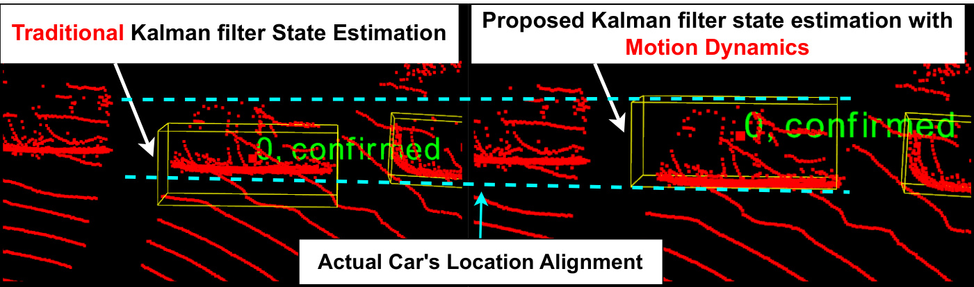
Figure 1: State estimation (yellow bounding box) of an off-scene car drifts away from the actual car location (disconnected lines) with the traditional Kalman filter. Meanwhile, the proposed Kalman filter with motion dynamics shows robust localization for the car.
图 1: 传统卡尔曼滤波器对场外车辆的状态估计(黄色边界框)会偏离实际车辆位置(断开的线条)。而采用运动动力学的改进卡尔曼滤波器则能实现稳健的车辆定位。
Given an object’s current location (measurement), classical methods use Bayesian filters, such as the Kalman Filter (KF), to estimate the object’s next position (state) with uncertainty, a process known as state prediction. The estimation of the object’s state is refined when a new measurement arrives, which is called a state update. In the literature of MOT methods, state prediction estimates the next state of an object based on a constant motion model, such as a constantvelocity or constant-acceleration model. The main limitation of these models is that they do not always reflect the motion status of the objects (motion dynamics). For instance, the state estimation of a car with no change in velocity while employing a constant velocity model has a better state estimation than the constant acceleration or jerk model (3rd derivative of motion equation), as presented in Figure 2 case A. On the other hand, when the car accelerates, as shown in Figure 2 case B, the constant jerk model has the lowest state estimation error for the car. Similarly, the constant acceleration model outperforms in state estimation when the car exhibits a change in velocity with slight to no change in acceleration, as shown in Figure 2 case C.
给定物体的当前位置(测量值),经典方法使用贝叶斯滤波器(如卡尔曼滤波器(KF))来估计物体的下一个位置(状态)及其不确定性,这一过程称为状态预测。当新的测量值到达时,会优化对物体状态的估计,这称为状态更新。在多目标跟踪(MOT)方法的文献中,状态预测基于恒定运动模型(如匀速或匀加速模型)来估计物体的下一个状态。这些模型的主要局限性在于它们并不总能反映物体的运动状态(运动动力学)。例如,如图2案例A所示,当汽车速度不变时,采用匀速模型的状态估计优于匀加速或加加速度模型(运动方程的三阶导数)。另一方面,如图2案例B所示,当汽车加速时,加加速度模型的状态估计误差最小。类似地,如图2案例C所示,当汽车速度变化而加速度几乎不变时,匀加速模型在状态估计中表现更优。
This behavior has been repeatedly observed in multiple scenarios, indicating that the precision of state estimation from a motion model depends on its alignment with the object’s current motion dynamics. The state estimation precision reduces as the motion dynamics do not match the employed motion model, eventually injecting noise into the state estimation process in the KF that impacts object localization, particularly occluded and off-scene objects, as demonstrated in Figure 1. This work proposes a novel formulation of the KF that accounts for objects’ motion dynamics and adaptively adjusts a dynamic motion model based on observed changes. The proposed solution shows precise state estimation localization (Figure 1) and less trajectory deviation for occluded and off-scene objects over the traditional KF, outperforming recent KITTI and Waymo Open Dataset (WOD) benchmarks.
这一现象在多个场景中被反复观察到,表明运动模型的状态估计精度取决于其与物体当前运动动态的匹配程度。当运动动态与所采用的运动模型不匹配时,状态估计精度会降低,最终在卡尔曼滤波 (KF) 的状态估计过程中引入噪声,从而影响物体定位,特别是被遮挡和离开场景的物体,如图 1 所示。本研究提出了一种新颖的卡尔曼滤波公式,该公式考虑了物体的运动动态,并根据观测到的变化自适应调整动态运动模型。所提出的解决方案在状态估计定位上表现出更高的精度 (图 1),并且相较于传统卡尔曼滤波,对于被遮挡和离开场景的物体具有更小的轨迹偏差,其性能超越了近期 KITTI 和 Waymo 开放数据集 (WOD) 的基准。
The contribution of this work can be summarized as follows:
本工作的贡献可概括如下:
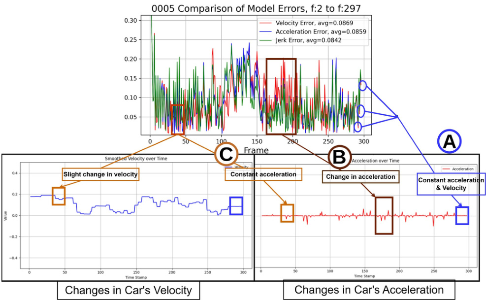
Figure 2: The graph demonstrates the performance fluctuation in state estimation for three motion models: constant velocity (Red), constant acceleration (Blue), and constant jerk (Green). The top graph compares the Euclidean distance error in state estimation obtained by the three models of the 0005 stream in the KITTI [2] dataset. The second row shows graphs of the car’s motion dynamics, change in velocity (Blue), and change in acceleration (Red).
图 2: 该图展示了三种运动模型在状态估计中的性能波动:匀速(红色)、匀加速(蓝色)和匀加加速(绿色)。顶部图表对比了KITTI数据集[2]中0005数据流通过三种模型获得的状态估计欧氏距离误差。第二行显示了车辆运动动力学图表,包括速度变化(蓝色)和加速度变化(红色)。
- As the opposite of the attempts in the literature, multiple motion models simultaneously, this work maintains the singularity of the assigned motion model that adaptively adjusted as per the captured motion dynamics, resulting in low latency with an average additional computational cost of $0.078\mathrm{ms}$ per frame (Table 4), making it efficient for real-time applications.
- 与文献中尝试同时使用多个运动模型的做法相反,本研究保持所分配运动模型的单一性,并根据捕获的运动动态进行自适应调整,从而实现了低延迟,平均每帧额外计算成本仅为 $0.078\mathrm{ms}$ (表4),使其适用于实时应用。
2 Related Work
2 相关工作
The KF is widely used in MOT literature [3–11], particularly for methods that follow tracking-by-detection paradigms. It predicts the state of tracked objects that nearly resample their actual location and motion states. An imprecise state prediction of an object can lead to failure in the association stage, where the object’s recent position is associated with the closest state prediction. Hence, motion model selection for state prediction in the KF becomes critical in the MOT literature, as it significantly affects tracking performance. The literature shows conflicting preferences for the proper motion model, which has consistently improved state prediction localization. Some methods [7, 8, 10–15] favor the constant velocity model, claiming its out performance over other motion models. At the same time, other methods [5, 6, 9] utilize the acceleration motion model, as the constant velocity motion model is too simplistic to handle maneuvering in tracking.
KF(卡尔曼滤波器)在MOT(多目标跟踪)文献[3-11]中被广泛使用,尤其适用于遵循检测跟踪范式的方法。它能预测被跟踪对象的状态,这些状态几乎复现了目标的实际位置和运动状态。若物体状态预测不准确,会导致关联阶段失败——该阶段需要将物体当前位置与最接近的状态预测相关联。因此,KF中用于状态预测的运动模型选择成为MOT文献中的关键因素,因为它显著影响跟踪性能。
文献显示对于最佳运动模型存在分歧观点,这些模型持续改进了状态预测的定位精度。部分方法[7,8,10-15]倾向于恒定速度模型,声称其性能优于其他运动模型;而另一些方法[5,6,9]则采用加速运动模型,认为恒定速度模型过于简单,无法处理跟踪中的机动动作。
For varied reasons, the velocity motion model in the KF is the most commonly used in MOT literature [7, 8, 10–15]. Some MOT methods [7, 10, 13, 14] employ a constant velocity model over others due to its simplicity that facilitates the integration into various frameworks in addition to its lower computational cost, which makes it an efficient choice for real-time systems. Another study [3] has shown that, in some cases, the constant velocity model outperforms higher-degree motion models. Similarly, Na et al. [4] have observed that the constant velocity model is more robust when the target acceleration is slight or unpredictable, especially in noisy environments.
由于多种原因,卡尔曼滤波器(KF)中的匀速运动模型是多目标跟踪(MOT)文献中最常用的方法[7, 8, 10–15]。部分MOT方法[7, 10, 13, 14]采用匀速模型而非其他模型,因其简单性便于集成到各类框架中,且计算成本较低,使其成为实时系统的高效选择。另一项研究[3]表明,在某些情况下,匀速模型表现优于高阶运动模型。类似地,Na等人[4]发现当目标加速度较小或不可预测时(尤其在噪声环境中),匀速模型具有更强的鲁棒性。
On the other hand, some recent MOT methods [5, 6, 9] adopt a constant acceleration motion model instead of a constant velocity. Part of the recent MOT methods [6, 9] claim that the constant velocity model is trivial and cannot predict precise positions for objects when they face dramatic velocity changes. Wu et al. [6] state that the prediction error accumulates from employing a constant velocity model, which increases exponentially as objects temporarily disappear due to occlusion. In the context of AVs, Reich et al. [9] underline that the maneuvering of a target object depends not only on the target motion but also on the ego motion of the AV. Even though some objects, like parked cars, seem to have no motion, an accelerated AV observes them as objects in motion equal to its motion, which still requires a constant acceleration motion model to handle the ego-motion maneuvering. Despite the maneuvering concerns for objects of MOT methods replacing constant velocity with an acceleration model for state prediction,
另一方面,部分近期多目标跟踪(MOT)方法[5,6,9]采用恒定加速度运动模型替代恒定速度模型。其中[6,9]指出恒定速度模型过于简单,在目标速度剧烈变化时无法准确预测位置。Wu等人[6]表明恒定速度模型会导致预测误差累积,当目标因遮挡暂时消失时误差呈指数级增长。针对自动驾驶车辆(AVs)场景,Reich等人[9]强调目标机动性不仅取决于目标运动,还需考虑AV自身运动。即使如停放车辆等看似静止的物体,加速中的AV也会将其视为与自身运动状态相同的运动物体,仍需恒定加速度模型来处理自车运动机动。尽管这些MOT方法关注机动性问题并采用加速度模型进行状态预测以替代恒定速度模型,
Nagy et al. [5] reveal that the tracking performance for occluded objects for MOT methods using constant acceleration can also miss recovering the objects after occlusion due to memory size constraints. The main issue with using a single motion model, either constant velocity or acceleration, is that the performance of state estimation degrades whenever the target’s motion dynamics do not match the assigned motion model, because the current KF formulation neglects motion dynamics.
Nagy等人[5]指出,由于内存大小限制,使用恒定加速度的MOT方法对遮挡物体的跟踪性能也可能在遮挡后无法恢复物体。使用单一运动模型(无论是恒定速度还是恒定加速度)的主要问题是,每当目标的运动动态与分配的运动模型不匹配时,状态估计的性能就会下降,因为当前的KF公式忽略了运动动态。
Further studies [3, 4] show that the motion model’s performance for tracking a target depends on the maneuvers demonstrated by the target. Na et al. [3] conduct experiments that show the constant velocity model is sufficient for non-maneuvering situations, while the constant acceleration model outperforms in maneuvering scenarios. Recent research [4, 16] attempts to tackle this issue by employing an interactive multi-model KF that uses multiple motion models simultaneously, with model selection based on an initial predefined probability for each model. Despite the improvement shown in state estimation, operating multiple motion models simultaneously is highly computationally expensive, particularly in multi-object tracking, where calculations for each model are performed for all targets, in addition to the difficulty of handling sudden motion changes.
进一步的研究 [3, 4] 表明,运动模型在目标跟踪中的性能取决于目标所展示的机动行为。Na 等人 [3] 进行的实验显示,恒速模型足以应对非机动场景,而恒加速模型在机动场景中表现更优。近期研究 [4, 16] 尝试通过采用交互式多模型卡尔曼滤波器 (KF) 来解决这一问题,该滤波器同时使用多个运动模型,并根据每个模型的初始预设概率进行模型选择。尽管在状态估计方面有所改进,但同时运行多个运动模型的计算成本极高,尤其是在多目标跟踪中,除了难以处理突然的运动变化外,还需为所有目标执行每个模型的计算。
Our investigation of the problem shows that the state estimation performance depends on the target’s motion dynamics. Figure 2 shows the state estimation performance of three motion models: velocity, acceleration, and jerk, of a car with many maneuvers. The performance of the jerk model peaks when the car is driving at mixed accelerations. Meanwhile, the acceleration model takes over as the car accelerates consistently. Lastly, the velocity motion model outperforms other models when the car’s velocity is consistent. This scenario shows the importance of considering the target motion dynamics for precise state estimation.
我们对问题的研究表明,状态估计性能取决于目标的运动动态。图 2 展示了进行多机动动作的汽车在三种运动模型(匀速、匀加速和加加速度)下的状态估计表现。当车辆处于混合加速度状态时,加加速度模型的表现达到峰值;当车辆持续加速时,匀加速模型则占据优势;而当车速保持稳定时,匀速运动模型的表现优于其他模型。这一场景揭示了考虑目标运动动态对实现精确状态估计的重要性。
This work addresses the limitation mentioned earlier by proposing a dynamic motion model with a novel formulation of the KF that accounts for the target motion dynamics and adaptively integrates them into the dynamic motion model, eliminating the need to operate multiple motion models while maintaining computational efficiency.
本工作针对前述局限性提出了一种动态运动模型,通过创新性地构建卡尔曼滤波器 (KF) 来捕捉目标运动动态特征,并将其自适应地整合到动态运动模型中,从而在保持计算效率的同时无需运行多个运动模型。
3 Methodology
3 方法论
This work addresses the limitations of current motion models and the neglect of object motion dynamics in the standard KF formulation by introducing a novel formulation of the KF state update and state prediction that considers the motion dynamics of objects in state estimation. Figure 3 shows a high-level overview of the pipeline of the proposed formulation of the KF incorporating object motion dynamics. Given an object observed at time $t-1$ , the object has three primary parameters: state estimation $\hat{x}{t-1|t-1}$ at time $t-1$ updated according to a measurement taken at time $t-1$ , the state estimation uncertainty covariance $P_{t-1|t-1}$ at time $t-1$ , and weighted motion dynamics $\hat{w}_{t-1|t-1}$ of the object at time $t-1$ updated based on a measurement taken at time $t-1$ .
本研究通过提出一种考虑物体运动动态的卡尔曼滤波(KF)状态更新与状态预测新公式,解决了当前运动模型的局限性以及标准KF公式中对物体运动动态的忽视问题。图3展示了融合物体运动动态的KF公式流程概览。给定在时间$t-1$观测到的物体,该物体具有三个主要参数:根据$t-1$时刻测量值更新的状态估计$\hat{x}{t-1|t-1}$,$t-1$时刻的状态估计不确定协方差$P_{t-1|t-1}$,以及基于$t-1$时刻测量值更新的物体加权运动动态$\hat{w}_{t-1|t-1}$。
At the prediction step, covered in Section 3.1, the model estimates the next state estimation $\hat{x}{t\mid t-1}$ of the object at time $t$ of measurement $t-1$ through the state-transition model $F_{t}$ . As shown in the estimated position state diagram in Figure 3, the state-transition model $F_{t}$ maps the state $\hat{x}{t-1|t-1}$ , highlighted by red dot-eclipse, to $\hat{x}{t\mid t-1}$ , marked by red eclipse; however, this transition is weighted by the estimated weights of object dynamics $\hat{w}{t-1}$ that adjusts the state according to the object motions, marked by blue eclipse. Thus, the obtained $\hat{x}{t\mid t-1}$ is the estimated state at time $t$ considering the latest dynamics observed at time $t-1$ . The state estimation uncertainty covariance will increase as the model becomes uncertain about the new estimate, obtaining an updated covariance $\hat{P}_{t|t-1}$ .
在预测步骤(见第3.1节)中,模型通过状态转移模型 $F_{t}$ 根据 $t-1$ 时刻的测量值估算 $t$ 时刻物体的下一状态估计 $\hat{x}{t\mid t-1}$。如图3的估计位置状态图所示,状态转移模型 $F_{t}$ 将红色点椭圆标记的状态 $\hat{x}{t-1|t-1}$ 映射到红色椭圆标记的 $\hat{x}{t\mid t-1}$;但该转移过程受蓝色椭圆标记的物体动态估计权重 $\hat{w}{t-1}$ 调节,该权重会根据物体运动调整状态。因此,所得 $\hat{x}{t\mid t-1}$ 是结合 $t-1$ 时刻最新动态观测的 $t$ 时刻估计状态。随着模型对新估计值的不确定性增加,状态估计不确定协方差将增大,从而获得更新的协方差 $\hat{P}_{t|t-1}$。
When a new measurement arrives $y_{t}$ at the following time frame $t$ , the estimated state $\hat{x}{t\mid t-1}$ will be compared and updated according to the new measurement at time $t$ of the object state to obtain a refined state estimation $\hat{x}{t\mid t}$ . Accordingly, the object dynamics are also updated as per the new measurement, which requires eliminating any noise impact on the measurement localization of the object, as discussed in Section 3.2. The noise mitigation term $D_{t}$ , introduced in [1], eliminates the localization noise from the employed detector.
当新测量值 $y_{t}$ 在下一时间帧 $t$ 到达时,预估状态 $\hat{x}{t\mid t-1}$ 将根据目标在 $t$ 时刻的新测量值进行比对和更新,从而得到优化后的状态估计 $\hat{x}{t\mid t}$。相应地,目标动态也会根据新测量值进行更新,这需要消除测量定位中噪声对目标的影响,如第3.2节所述。文献[1]引入的噪声抑制项 $D_{t}$ 可消除所用检测器的定位噪声。
Next, a Gaussian distribution of motion dynamics of the object observed through a time window called the ”Smoothing window”, discussed in Section 3.4, is formed for each motion dynamic term in the motion model used in the prediction step. In this case, we use a motion model consisting of the position’s first three derivatives (Jerk motion model). Thus, the three Gaussian distribution dynamics shown in the updated motion dynamics graph in Figure 3 represent the change in position (first derivative), change in velocity (second derivative), and change in acceleration
接下来,通过一个称为"平滑窗口"(Smoothing window)的时间窗口(详见第3.4节)观测到的物体运动动态,会为预测步骤中使用的运动模型中的每个动态项形成一个高斯分布。在本研究中,我们采用了包含位置前三阶导数(Jerk运动模型)的运动模型。因此,图3更新后的运动动态图中显示的三个高斯分布动态分别代表:位置变化(一阶导数)、速度变化(二阶导数)和加速度变化。
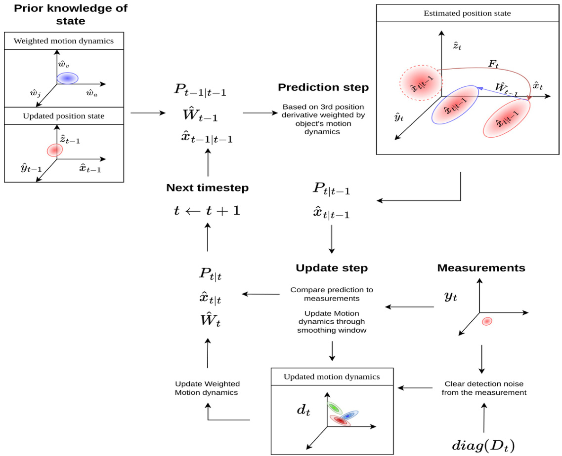
Figure 3: The diagram shows an overview of the proposed Kalman filter incorporating motion dynamics. The flow begins with the prior knowledge of an object’s states at time $t-1$ . The information includes state uncertainty $P_{t-1|t-1}$ , weighted motion dynamics of the object $\hat{W}{t-1}$ , and object’s state $\hat{x}{t-1|t-1}$ . This information is used to predict the next state estimation of the object, considering its captured motion dynamics, and adjust the estimated state accordingly. This results in the next state estimation $\hat{x}{t\mid t-1}$ and an updated uncertainty $P_{t|t-1}$ . With a new measurement, the object’s spatial state will be updated to obtain $\hat{x}{t\mid t}$ , and new motion dynamics will be captured through the Gaussian distribution of changes observed in motion dynamics parameters (Position, velocity, and acceleration). The obtained updated motion dynamics $d_{t}$ from the Gaussian distribution is weighted to form an updated weighted motion dynamics $\hat{W}_{t}$ . The flow will be repeated in the next time step $t+1$ .
图 3: 该图展示了融合运动动力学的卡尔曼滤波器 (Kalman filter) 整体流程。流程始于物体在时间 $t-1$ 的状态先验知识,包括状态不确定性 $P_{t-1|t-1}$ 、加权运动动力学 $\hat{W}{t-1}$ 以及物体状态 $\hat{x}{t-1|t-1}$ 。这些信息用于预测物体下一状态估计值,同时考虑其捕获的运动动力学并相应调整估计状态,最终得到下一状态估计 $\hat{x}{t\mid t-1}$ 和更新后的不确定性 $P_{t|t-1}$ 。当获得新测量值时,物体空间状态将更新为 $\hat{x}{t\mid t}$ ,并通过运动动力学参数 (位置、速度、加速度) 变化的高斯分布捕获新运动动力学。从高斯分布中获取的更新后运动动力学 $d_{t}$ 经过加权形成更新后的加权运动动力学 $\hat{W}_{t}$ 。该流程将在下一时间步 $t+1$ 重复执行。
(third derivative).
(三阶导数).
The motion dynamics of the object $d_{t}$ at time $t$ will be adjusted according to the obtained Gaussian distributions of the object’s motion dynamics. Then, the weighted motion dynamics $\hat{w}{t}$ will be updated based on the new observed motion dynamics $d_{t}$ based on measurement $y_{t}$ at time $t$ . Finally, the state estimation uncertainty covariance $\hat{P}{t|t-1}$ decreases as new information about the object’s state is observed, in the form of measurement $y_{t}$ , to obtain an updated covariance $\hat{P}_{t|t}$ . Lastly, the procedures will be repeated at each time stamp.
物体在时间 $t$ 的运动动态 $d_{t}$ 将根据获得的运动动态高斯分布进行调整。随后,基于时间 $t$ 的测量值 $y_{t}$ 观测到的新运动动态 $d_{t}$ ,加权运动动态 $\hat{w}{t}$ 将被更新。最后,随着以测量值 $y_{t}$ 形式观测到物体状态的新信息,状态估计不确定协方差 $\hat{P}{t|t-1}$ 会减小,从而得到更新后的协方差 $\hat{P}_{t|t}$ 。上述步骤将在每个时间戳重复执行。
3.1 Motion Dynamics in State Prediction
3.1 状态预测中的运动动力学
The subsequent estimated state should consider the objects’ motion dynamics at the prediction step. In this work, we use the third derivative of the motion equation (Jerk motion equation), which consists of the object’s position, velocity, acceleration, and changes in acceleration (Jerk), as shown in Equation 1.
随后的估计状态应考虑物体在预测步骤中的运动动力学。在本研究中,我们采用运动方程的三阶导数(Jerk运动方程),该方程包含物体的位置、速度、加速度及加速度变化率(Jerk),如公式1所示。
$$
x(t)=x_{t}+v_{t}t+{\frac{1}{2}}a_{t}t^{2}+{\frac{1}{6}}j_{t}t^{3}
$$
$$
x(t)=x_{t}+v_{t}t+{\frac{1}{2}}a_{t}t^{2}+{\frac{1}{6}}j_{t}t^{3}
$$
The main problem of using Equation 1 as a motion model for state prediction in the KF is the assumption of observing the object’s motion state velocity $v_{t}$ , acceleration $a_{t}$ , and jerk $j_{t}$ as the absolute motion state of the object. However, this assumption is not valid as the motion state of the object is influenced by the process noise and measurement
将方程1作为卡尔曼滤波器(KF)中状态预测的运动模型的主要问题在于:其假设观测到的物体运动状态速度$v_{t}$、加速度$a_{t}$和加加速度$j_{t}$代表物体的绝对运动状态。然而这一假设并不成立,因为物体的运动状态会受到过程噪声和测量噪声的影响。
noise from the update state in the KF. For instance, if a stationary object is observed, its motion state in the KF will still have values for $v_{t},a_{t}$ , and $j_{t}$ , leading to a slight deviation of the predicted bounding box. This deviation in prediction accumulates, particularly for occluded objects.
卡尔曼滤波器 (KF) 更新状态中的噪声。例如,当观测到静止物体时,其在 KF 中的运动状态仍会包含 $v_{t},a_{t}$ 和 $j_{t}$ 的数值,导致预测边界框出现轻微偏差。这种预测偏差会不断累积,尤其对于被遮挡物体更为明显。
To tackle this issue while maintaining the singularity of the motion model, Equation 1 is weighted by the weighted motion dynamics of the target object $\hat{w}_{t}$ as shown in Equation 2.
为解决这一问题,同时保持运动模型的单一性,如式2所示,将式1乘以目标物体的加权运动动力学 $\hat{w}_{t}$。
$$
x(t)=x_{0}+(\hat{w_{v}}.v_{t})t+\frac{1}{2}(\hat{w_{a}}.a_{t})t^{2}+\frac{1}{6}(\hat{w_{j}}.j_{t})t^{3}
$$
$$
x(t)=x_{0}+(\hat{w_{v}}.v_{t})t+\frac{1}{2}(\hat{w_{a}}.a_{t})t^{2}+\frac{1}{6}(\hat{w_{j}}.j_{t})t^{3}
$$
$\hat{w_{v}},\hat{w_{a}}$ , and $\hat{w}{j}$ represent the amount of change in the object motion to the motion parameters. For instance, $\hat{w_{v}}=$ $\hat{w_{a}}=\hat{w_{j}}=0$ when the observed object is in a stationary state (no motion). In motion, the weight value will change up to the extent of the changes observed in position, velocity, and acceleration, and the motion model will be adjusted to match the object’s observed motion dynamics. These motion dynamics can be used to formulate the matrix $\hat{W}_{t}$ , representing the target object’s recent dynamics at time $t$ .
$\hat{w_{v}}$、$\hat{w_{a}}$ 和 $\hat{w_{j}}$ 表示物体运动对运动参数的变化量。例如,当观测对象处于静止状态(无运动)时,$\hat{w_{v}} = \hat{w_{a}} = \hat{w_{j}} = 0$。在运动过程中,权重值会根据观测到的位置、速度和加速度变化程度进行调整,运动模型也将被修正以匹配物体的观测运动动态。这些运动动态可用于构建矩阵 $\hat{W}_{t}$,该矩阵表示目标物体在时间 $t$ 的最新动态。
$$
\hat{W_{t}}=\left[\begin{array}{c c c c}{1}&{0}&{0}&{0}\ {0}&{\hat{w_{v}}}&{0}&{0}\ {0}&{0}&{\hat{w_{a}}}&{0}\ {0}&{0}&{0}&{\hat{w_{j}}}\end{array}\right]
$$
$$
\hat{W_{t}}=\left[\begin{array}{c c c c}{1}&{0}&{0}&{0}\ {0}&{\hat{w_{v}}}&{0}&{0}\ {0}&{0}&{\hat{w_{a}}}&{0}\ {0}&{0}&{0}&{\hat{w_{j}}}\end{array}\right]
$$
Accordingly, the next state prediction of the KF can be presented as follows:
因此,KF (Kalman Filter) 的下一状态预测可表示如下:
$$
\hat{\mathbf{x}}{\mathbf{t}|\mathbf{t}-\mathbf{1}}=\mathbf{F}{\mathbf{t}}\hat{\mathbf{W}}{\mathbf{t}-\mathbf{1}}\hat{\mathbf{x}}_{\mathbf{t}-\mathbf{1}|\mathbf{t}-\mathbf{1}}
$$
$$
\hat{\mathbf{x}}{\mathbf{t}|\mathbf{t}-\mathbf{1}}=\mathbf{F}{\mathbf{t}}\hat{\mathbf{W}}{\mathbf{t}-\mathbf{1}}\hat{\mathbf{x}}_{\mathbf{t}-\mathbf{1}|\mathbf{t}-\mathbf{1}}
$$
Where $F_{t}\hat{W}{t-1}$ maps the current state $\hat{x}{t-1|t-1}$ to the next state $\hat{x}_{t\mid t-1}$ based on measurement $t-1$ by considering the objects motion dynamics observed at time $t-1$ .
其中 $F_{t}\hat{W}{t-1}$ 将当前状态 $\hat{x}{t-1|t-1}$ 映射到下一状态 $\hat{x}_{t\mid t-1}$ ,这是基于时间 $t-1$ 的测量值,并考虑了在时间 $t-1$ 观测到的物体运动动力学。
3.2 Localization Term Selection for Motion Dynamics
3.2 运动动力学的定位术语选择
Acquiring data that perceives the motion dynamics of objects is a critical part of this work. Neglecting the motion dynamics can lead to dramatic drift in the estimated state of the objects. The motion dynamics of an object can be perceived across consecutive measurements of its states. As shown in Equation 5, acquiring and perceiving the amount of change in position and velocity requires at least three successive position states of the object, assuming $z$ is the object’s actual position.
获取能够感知物体运动动态的数据是这项工作的关键部分。忽略运动动态会导致物体估计状态出现显著漂移。通过连续测量物体状态可以感知其运动动态。如公式5所示,假设$z$为物体实际位置,获取并感知位置和速度的变化量至少需要该物体三个连续的位置状态。
$$
\begin{array}{r l}&{\mathrm{Velocity:}\quad\Delta z_{t}=z_{t}-z_{t-1},}\ &{\sigma_{\Delta z_{t}}\propto\mathrm{accelerationfluctuations},}\ &{\mathrm{Acceleration:}\quad\Delta^{2}z_{t}=\Delta z_{t}-\Delta z_{t-1},}\ &{\sigma_{\Delta^{2}z_{t}}\propto\mathrm{jerkfuctuations}.}\end{array}
$$
$$
\begin{array}{r l}&{\text{速度:}\quad\Delta z_{t}=z_{t}-z_{t-1},}\ &{\sigma_{\Delta z_{t}}\propto\text{加速度波动},}\ &{\text{加速度:}\quad\Delta^{2}z_{t}=\Delta z_{t}-\Delta z_{t-1},}\ &{\sigma_{\Delta^{2}z_{t}}\propto\text{加加速度波动}.}\end{array}
$$
Equation 5 computes the amount of change required to provide an estimation of the motion dynamics for the jerk motion model, as discussed in Section 3.3; however, an accurate measurement of the objects’ position $z_{t}$ is needed to obtain it. Since the actual position of the objects is unavailable, $z_{t}$ can be replaced by three potential terms representing the objects’ position state. The first option is the measurement from the employed detector, $\mathbf{z_{t}}$ , at time $t$ . The second option is the updated state estimation $\mathbf{x_{t|t}}$ of measurement $t$ at time $t$ . The third option is to use detection measurement $\mathbf{z_{t}}$ (from the first option) and use the noise mitigation detection $\mathbf{D_{t}}$ proposed in [1] to remove any noise coming from the detector (Post measurement).
方程5计算了为急动运动模型提供运动动态估计所需的变化量,如第3.3节所述;然而,需要准确测量物体位置$z_{t}$才能获得该值。由于物体的实际位置不可用,$z_{t}$可以用表示物体位置状态的三个潜在项替代。第一个选项是所采用检测器在时间$t$的测量值$\mathbf{z_{t}}$。第二个选项是时间$t$对测量$t$的更新状态估计$\mathbf{x_{t|t}}$。第三个选项是使用检测测量值$\mathbf{z_{t}}$(来自第一个选项),并采用[1]中提出的噪声抑制检测$\mathbf{D_{t}}$来消除检测器产生的任何噪声(后测量)。
To determine which term better represents the objects’ actual location, an experiment is conducted on the KITTI [2] dataset across multiple streams, evaluating the localization performance of each term to the objects’ actual locations from the ground truth. At each timestamp, each term is computed for all objects, and the localization error is calculated using Euclidean distance to the actual location of these objects.
为确定哪个术语能更准确地表示物体的实际位置,我们在KITTI [2] 数据集上进行了多组流数据的实验,评估各术语相对于地面真实值中物体实际位置的定位性能。在每个时间戳,计算所有物体的各术语值,并通过与物体实际位置的欧氏距离来计算定位误差。
Figure 4 shows a graphical representation of the Euclidean distance error between the localization obtained from each term discussed earlier and the actual localization of two cars from the ground truth localization. The post-measurement term shows the closest capture of the car’s localization to the ground truth, achieving the lowest mean square error and standard deviation, which matches the observations in work [1].
图 4 展示了从先前讨论的每个定位项获得的定位与两辆车的真实定位之间的欧氏距离误差的图形表示。测量后项显示出对车辆定位最接近真实值的捕捉,实现了最低的均方误差和标准差,这与文献 [1] 中的观察结果一致。
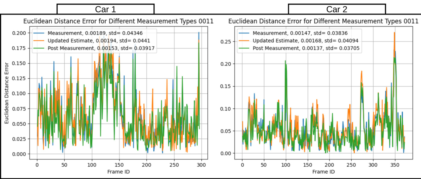
Figure 4: The graph shows the Euclidean distance error comparison between the localization measurements obtained from the employed detector (Blue-line), the updated state estimation of the object’s location (Orange-line), and the measurement from the detector with cleared noise by the proposed term $D_{t}$ (Green-line). The experiment is conducted in two cars over more than 300 consecutive frames. The numerical values in the legend present the mean square error and standard deviation, respectively.
图 4: 该图展示了采用检测器获得的定位测量值(蓝线)、物体位置的更新状态估计(橙线)以及通过提出的 $D_{t}$ 项消除噪声后的检测器测量值(绿线)之间的欧氏距离误差对比。实验在两辆车上进行了超过300帧的连续测试。图例中的数值分别表示均方误差和标准差。
To this end, the post-measurement (third) term is used to determine the recent position of objects. The term is computed by eliminating the localization noise from the detector $D_{t}$ , as presented in [1], from the measurement $z_{t}$ and obtaining the post-measurement localization $\hat{z}_{t}$ .
为此,后测量(第三)项用于确定物体的最近位置。该项通过从检测器 $D_{t}$ 中消除定位噪声(如文献[1]所述),从测量值 $z_{t}$ 中计算得出,并获取后测量定位 $\hat{z}_{t}$。
$$
\hat{\bf z_{t}}={\bf z_{t}}-\left({\bf H}{\bf K_{t}}\right)\mathrm{diag}({\bf D_{t}})
$$
$$
\hat{\bf z_{t}}={\bf z_{t}}-\left({\bf H}{\bf K_{t}}\right)\mathrm{diag}({\bf D_{t}})
$$
As shown in Equation 6, Kalman gain $\mathbf{K_{t}}$ is incorporated into the noise residual, $\mathrm{diag(\mathbf{D}{t})}$ , to include the model uncertainty while clearing the noise from the measurement. Since $\mathbf{K_{t}}$ is in the estimation space, $\mathbf{H}$ maps it to the measurement space. Finally, the obtained refinement noise is removed from the measurement.
如式6所示,卡尔曼增益 $\mathbf{K_{t}}$ 被纳入噪声残差 $\mathrm{diag(\mathbf{D}{t})}$ 中,在消除测量噪声的同时引入模型不确定性。由于 $\mathbf{K_{t}}$ 位于估计空间,$\mathbf{H}$ 将其映射至测量空间。最终从测量值中移除了所得到的修正噪声。
3.3 Temporal Evolution in Motion Dynamics Estimation
3.3 运动动力学估计中的时间演化
As shown in Equation 5, three consecutive observations of an object’s position are used to quantify the fluctuation in an object’s velocity and acceleration motion dynamics. Nevertheless, a single quant if i cation is insufficient to conclude an object’s motion dynamics since external noise could impact the measurement $z_{t}$ . A distribution of multiple quant if i cations can provide a more accurate estimation of an object’s motion dynamics. The distribution of consecutive quant if i cations of motion dynamics parameters (position $z_{t}$ , velocity $\Delta z_{t}$ , and acceleration $\Delta^{2}z_{t}$ ) of an object, obtained from Equation 5, resamples a 2D Gaussian distributions in $\mathbf{X}$ and y directions, as shown in Figure 3 (Updated motion dynamics). The distribution of each motion dynamics parameter shapes a Gaussian distribution around its potential value.
如公式5所示,通过物体位置的连续三次观测来量化其速度和加速度运动动态的波动。然而,单次量化不足以确定物体的运动动态,因为外部噪声可能影响测量值$z_{t}$。多次量化的分布能更准确地估计物体运动动态。根据公式5获得的物体运动动态参数(位置$z_{t}$、速度$\Delta z_{t}$和加速度$\Delta^{2}z_{t}$)连续量化分布,在$\mathbf{X}$和y方向上重采样为二维高斯分布,如图3(更新后的运动动态)所示。每个运动动态参数的分布在其潜在值周围形成高斯分布。
To obtain an estimation of an object’s motion dynamics, consider a single motion parameter: fluctuation in velocity $\sigma_{\Delta z_{t}}$ . Assume a car drives at a constant velocity. The amount of change in position (traveling distance) value $\Delta z_{t\leftarrow s}$ from time $s$ to time $t$ will remain constant, which refers to the mean of the distribution $\Delta\bar{z}$ . In this case, the deviation of the data $\sigma_{\Delta z_{t\leftarrow s}}$ from the mean will be approximately zero. On the other hand, if the car starts to drive at a variable velocity, the amount of change in position will change over time. In this case, the deviation of the data from the mean increases as the variation in velocity increases. Thus, the standard deviation $\sigma_{\Delta z_{t\leftarrow s}}$ approximates the fluctuation in the velocity motion dynamics of the object from time $s$ to time $t$ . Given the consecutive readings and the gradual behavior of objects’ motion, the formulation will shape a Gaussian distribution.
为估算物体的运动动态,考虑单一运动参数:速度波动 $\sigma_{\Delta z_{t}}$。假设汽车以恒定速度行驶,从时刻 $s$ 到时刻 $t$ 的位置变化量(行驶距离)$\Delta z_{t\leftarrow s}$ 将保持恒定,即分布均值 $\Delta\bar{z}$。此时数据与均值的偏差 $\sigma_{\Delta z_{t\leftarrow s}}$ 近似为零。反之,若汽车以变速行驶,位置变化量将随时间改变,此时数据与均值的偏差会随速度变化幅度增大而增加。因此标准差 $\sigma_{\Delta z_{t\leftarrow s}}$ 可近似表征物体从时刻 $s$ 到时刻 $t$ 的速度运动动态波动。鉴于连续读数与物体运动的渐进特性,该公式将形成高斯分布。
In other words, the standard deviation $\sigma_{\Delta z_{t\leftarrow s}}$ increases when the car accelerates, resulting in varying travel distance changes over time. This increased variance in traveling distance widens the Gaussian distribution, thereby enlarging $\sigma_{\Delta z_{t\leftarrow s}}$ . Hence, $\sigma_{\Delta z_{t\leftarrow s}}$ reflects not only changes in velocity but also quantifies fluctuations in acceleration. Generalizing this relationship to motion dynamics parameters (velocity $\Delta z$ , acceleration $\Delta^{2}z$ ), the motion dynamics for observations from time $s$ to $t$ (with $k=t-s+1$ total observations) are estimated as:
换句话说,标准差 $\sigma_{\Delta z_{t\leftarrow s}}$ 会随着车辆加速而增大,导致行驶距离随时间变化。这种行驶距离方差的增大会拓宽高斯分布,从而扩大 $\sigma_{\Delta z_{t\leftarrow s}}$ 。因此,$\sigma_{\Delta z_{t\leftarrow s}}$ 不仅反映速度变化,还能量化加速度波动。将这一关系推广到运动动力学参数(速度 $\Delta z$、加速度 $\Delta^{2}z$),从时间 $s$ 到 $t$ 的观测数据(共 $k=t-s+1$ 次观测)的运动动力学估计为:
$$
\begin{array}{l}{\displaystyle\sigma(\Delta\theta_{t\leftarrow s})=\sqrt{\frac{1}{\displaystyle k-1}\sum_{i=1}^{k}\left(\Delta\theta_{i}-\overline{{\Delta\theta}}\right)^{2}},}\ {\displaystyle\mathrm{where}\Delta\theta\in{\Delta z,\Delta^{2}z},}\ {\displaystyle\overline{{\Delta\theta}}=\frac{1}{\displaystyle k}\sum_{i=1}^{k}\Delta\theta_{i}.}\end{array}
$$
$$
\begin{array}{l}{\displaystyle\sigma(\Delta\theta_{t\leftarrow s})=\sqrt{\frac{1}{\displaystyle k-1}\sum_{i=1}^{k}\left(\Delta\theta_{i}-\overline{{\Delta\theta}}\right)^{2}},}\ {\displaystyle\mathrm{where}\Delta\theta\in{\Delta z,\Delta^{2}z},}\ {\displaystyle\overline{{\Delta\theta}}=\frac{1}{\displaystyle k}\sum_{i=1}^{k}\Delta\theta_{i}.}\end{array}
$$
Here, $\Delta\theta_{t\leftarrow s}$ represents the finite differences of velocity $(\Delta z)$ or acceleration $({\mit\Delta}^{2}z)$ over the time window $t\leftarrow s$ , and $\overline{{\Delta\theta}}$ denotes their sample mean. The standard deviation $\sigma(\Delta\theta_{t\leftarrow s})$ quantifies fluctuations in the corresponding motion parameter.
这里,$\Delta\theta_{t\leftarrow s}$ 表示速度 $(\Delta z)$ 或加速度 $({\mit\Delta}^{2}z)$ 在时间窗口 $t\leftarrow s$ 内的有限差分,$\overline{{\Delta\theta}}$ 表示它们的样本均值。标准差 $\sigma(\Delta\theta_{t\leftarrow s})$ 量化了相应运动参数的波动。
The motion dynamics estimation vector $d_{t}$ is then derived as:
运动动态估计向量 $d_{t}$ 的计算公式为:
$$
d_{t}=\left[\begin{array}{c}{{1}}\ {{\sigma(z_{t\leftarrow s})}}\ {{\sigma(\Delta z_{t\leftarrow s})}}\ {{\sigma(\Delta^{2}z_{t\leftarrow s})}}\end{array}\right],
$$
$$
d_{t}=\left[\begin{array}{c}{{1}}\ {{\sigma(z_{t\leftarrow s})}}\ {{\sigma(\Delta z_{t\leftarrow s})}}\ {{\sigma(\Delta^{2}z_{t\leftarrow s})}}\end{array}\right],
$$
matri
矩阵
$$
\begin{array}{r l}{\sigma(z_{t\leftarrow s})}&{{}{\mathrm{captures position fluctuations,}}}\ {\sigma(\Delta z_{t\leftarrow s})}&{{}{\mathrm{corresponds to velocity~fluctuations,}}}\ {\sigma(\Delta^{2}z_{t\leftarrow s})}&{{}{\mathrm{reflects acceleration fluctuations.}}}\end{array}
$$
$$
\begin{array}{r l}{\sigma(z_{t\leftarrow s})}&{{}{\mathrm{captures position fluctuations,}}}\ {\sigma(\Delta z_{t\leftarrow s})}&{{}{\mathrm{corresponds to velocity~fluctuations,}}}\ {\sigma(\Delta^{2}z_{t\leftarrow s})}&{{}{\mathrm{reflects acceleration fluctuations.}}}\end{array}
$$
3.4 Motion Dynamics Transition and Smoothing Window
3.4 运动动力学过渡与平滑窗口
As demonstrated in Equation 7, the estimation of motion dynamics can be obtained from the distribution of $\sigma(\Delta\theta_{t\leftarrow s})$ across $k$ consecutive measurements. The determination of $k$ , called transition window size, should be carefully selected as it controls when the model alternates from one motion dynamic state to another.
如公式7所示,运动动态的估计可以通过连续k次测量中$\sigma(\Delta\theta_{t\leftarrow s})$的分布获得。其中k值(称为过渡窗口大小)的确定需要谨慎选择,因为它控制着模型从一个运动动态状态切换到另一个状态的时机。
For a better understanding of the motion dynamic transition and its influence on the state estimation, Figure 5 shows a use case of a car that accelerates and then decelerates. The car starts to accelerate at frame 140 to 160, as shown in the second graph when the change in distance shifts. The error in state estimation of the constant acceleration and jerk models decreases as expected, while increasing for the constant velocity model. From frame 160 to 168, there is a transition in the motion dynamics as the car starts to decelerate. At the transition state, the constant velocity yields the lowest error as the change in velocity approaches 0. This transition state is essential to consider while selecting the size of the transition window $k$ . The large window size can cause the failure to capture changes in motion dynamics that occur quickly, as shown in the transition state of Figure 5. On the other hand, a window that is too small can cause quick motion state transitions, which also impact the stability of the estimated state.
为了更好地理解运动动态转变及其对状态估计的影响,图5展示了一辆汽车加速后减速的用例。如第二张图表所示,当距离变化发生偏移时,车辆在140至160帧期间开始加速。恒定加速度和加加速度模型的状态估计误差如预期般下降,而恒定速度模型的误差则增大。在160至168帧期间,随着车辆开始减速,运动动态发生转变。在过渡状态下,由于速度变化趋近于0,恒定速度模型的误差最小。选择过渡窗口大小$k$时必须重点考虑这种过渡状态。如图5的过渡状态所示,过大的窗口尺寸可能导致无法快速捕捉运动动态的变化。另一方面,过小的窗口会引起运动状态快速切换,同样会影响估计状态的稳定性。
The transition window size $k$ determines how many observations are needed to gather adequate information about the object’s motion dynamics. The window size controls the motion dynamics weights, as presented in Equation 3, which adjusts the state estimation based on the observed motion dynamics. Figure 6 shows how different transition window sizes impact the motion dynamics weights presented in Equation 3.
过渡窗口大小 $k$ 决定了需要多少观测值才能收集足够的物体运动动态信息。如公式3所示,窗口大小控制着运动动态权重,该权重会根据观测到的运动动态调整状态估计。图6展示了不同过渡窗口大小如何影响公式3中的运动动态权重。
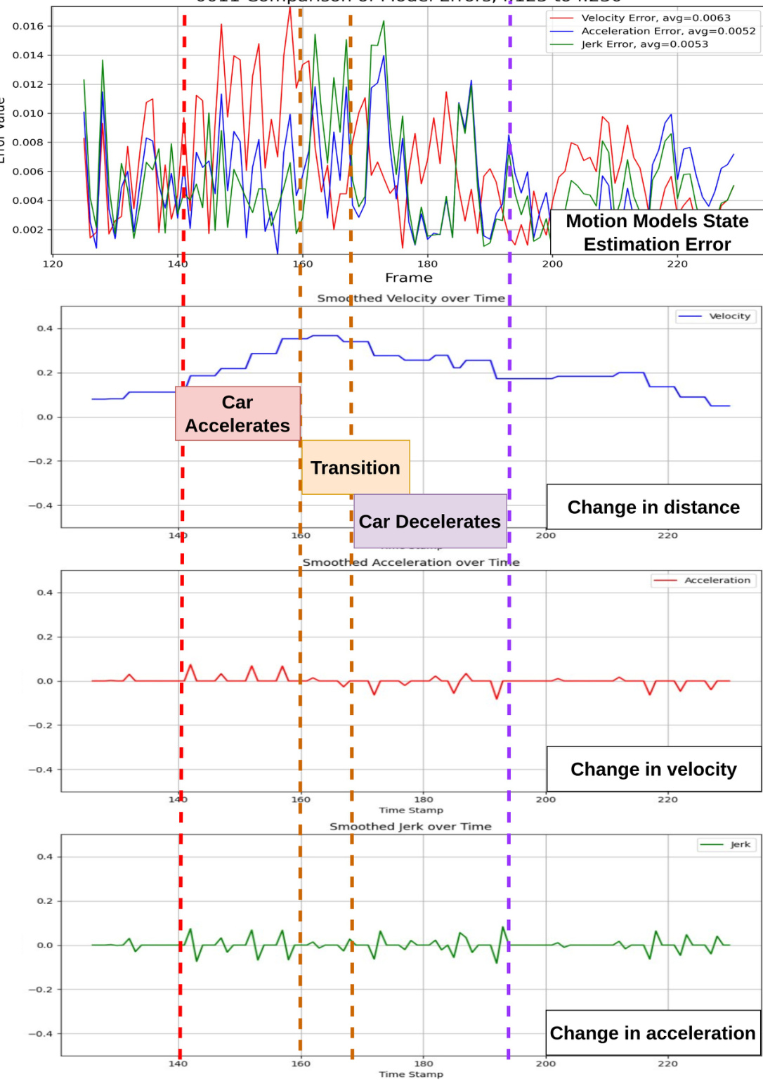
0011 Comparison of Model Errors,f:125tof:230 Figure 5: The graphs show a car’s motion dynamics, which accelerates and decelerates for a particular time stamp. The first graph shows the Euclidean distance error of state estimation from three different motion models: constant velocity (Red), constant acceleration (Blue), and constant Jerk (Green). The second graph shows the corresponding change in traveling distances from the ground truth, presenting the car motion dynamics for velocity. Meanwhile, the third graph shows the car’s velocity change compared to the ground truth, illustrating the motion dynamics for acceleration. The last graph shows the change in car acceleration from the ground truth, illustrating the motion dynamics for jerk. The graph highlights three transition states in the motion dynamics of the car: Acceleration (Red dot-line), transition from acceleration to deceleration (Orange dot-line), and deceleration (Violet dot-line).
图 5: 图表展示了车辆在特定时间戳下的加减速运动动态。第一幅图呈现了三种不同运动模型的状态估计欧氏距离误差:匀速(红色)、匀加速(蓝色)和匀加加速度(绿色)。第二幅图显示了与真实轨迹相比的行进距离变化,反映车辆速度维度的运动动态。第三幅图展示了车辆速度相对于真实值的变化,体现加速度维度的运动动态。最后一幅图呈现车辆加速度与真实值的偏差,展示加加速度维度的运动动态。图中特别标注了车辆运动动态的三个过渡状态:加速阶段(红色虚线)、加速转减速过渡阶段(橙色虚线)和减速阶段(紫色虚线)。
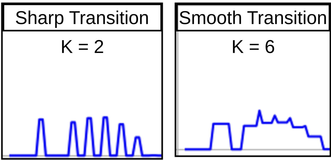
Figure 6: The graphs show the impact of the smoothing window of sizes 2 and 6 on the motion dynamics weight that responds to transitions between motion models. With a small smoothing window, the transition between models becomes sharp, causing an immediate switch; on the other hand, a larger window size shows smoother transitions.
图 6: 图表展示了大小为2和6的平滑窗口对响应运动模型间转换的运动动态权重的影响。较小的平滑窗口会使模型间转换变得尖锐,导致立即切换;而较大的窗口则呈现更平滑的过渡。
4 Weighted Motion Dynamics Evolution for State Update
4 状态更新的加权运动动态演化
The obtained motion dynamics vector $d_{t}$ cannot be used directly as weights into the motion parameters in Equation 2 because the standard deviation values can be between $[0,\infty[$ , they must be normalized to be in the range $[0,1]$ . For instance, constant velocity motion model can obtained from Equation 2 when $\hat{w}{a}=\hat{w}{j}=0$ . Meanwhile, the constant acceleration model can be obtained when $\hat{w}{j}=0$ . Hence, the primary purpose of the weights is to alternate between the three derivative models. Thus, the amount of change the model needs to alternate from one motion model to another must be determined, which will be used to normalize $d_{t}$ . This amount of change is called the motion dynamics factor donated by $\ell_{t}$ , which should be fine-tuned for all three derivatives. Assuming a one-dimensional space, the motion dynamic factor will be:
获得的运动动态向量 $d_{t}$ 不能直接作为方程2中运动参数的权重,因为标准差值可能介于 $[0,\infty[$ 之间,必须将其归一化到 $[0,1]$ 范围内。例如,当 $\hat{w}{a}=\hat{w}{j}=0$ 时,可从方程2得到匀速运动模型;而当 $\hat{w}{j}=0$ 时,则可得到匀加速运动模型。因此,权重的主要作用是在三个导数模型之间切换。需要确定模型从一个运动模型切换到另一个运动模型所需的变化量,该变化量将用于归一化 $d_{t}$。这个变化量称为运动动态因子,记作 $\ell_{t}$,应对所有三个导数进行微调。假设为一维空间,运动动态因子为:
$$
\ell_{t}=[1\quad\ell_{v}\quad\ell_{a}\quad\ell_{j}]
$$
$$
\ell_{t}=[1\quad\ell_{v}\quad\ell_{a}\quad\ell_{j}]
$$
Accordingly, the weighted motion dynamics are obtained as:
因此,加权运动动力学可表示为:
$$
\begin{array}{r l}&{\hat{w}{v}=\operatorname*{min}\left(\frac{\sigma\left(z_{t\rightarrow k}\right)}{\ell_{v}},1\right),}\ &{\hat{w}{a}=\operatorname*{min}\left(\frac{\sigma\left(\Delta z_{t\rightarrow k}\right)}{\ell_{a}},1\right),}\ &{\hat{w}{j}=\operatorname*{min}\left(\frac{\sigma\left(\Delta^{2}z_{t\rightarrow k}\right)}{\ell_{j}},1\right).}\end{array}
$$
$$
\begin{array}{r l}&{\hat{w}{v}=\operatorname*{min}\left(\frac{\sigma\left(z_{t\rightarrow k}\right)}{\ell_{v}},1\right),}\ &{\hat{w}{a}=\operatorname*{min}\left(\frac{\sigma\left(\Delta z_{t\rightarrow k}\right)}{\ell_{a}},1\right),}\ &{\hat{w}{j}=\operatorname*{min}\left(\frac{\sigma\left(\Delta^{2}z_{t\rightarrow k}\right)}{\ell_{j}},1\right).}\end{array}
$$
The normalization procedure can be formalized algebraically as matrix operations, as shown in Equation 10.
归一化过程可以用矩阵运算形式化表示,如式 10 所示。
$$
\begin{array}{l}{{\displaystyle{d_{t_{\mathrm{norm}}}=d_{t}\circ\ell_{t}^{-1}},}}\ {{\displaystyle{\hat{\pmb w}{t}=\frac{1}{2}\left({\bf1}{n}+d_{t_{\mathrm{norm}}}-|{\bf1}{n}-d_{t_{\mathrm{norm}}}|\right).}}}\end{array}
$$
$$
\begin{array}{l}{{\displaystyle{d_{t_{\mathrm{norm}}}=d_{t}\circ\ell_{t}^{-1}},}}\ {{\displaystyle{\hat{\pmb w}{t}=\frac{1}{2}\left({\bf1}{n}+d_{t_{\mathrm{norm}}}-|{\bf1}{n}-d_{t_{\mathrm{norm}}}|\right).}}}\end{array}
$$
By Equation 10, the weights are updated by the current evolution in the motion dynamics of objects.
根据公式10,权重通过物体运动动态的当前演变进行更新。
5 Results and Discussion
5 结果与讨论
This work proposes a formulation of the KF that accounts for the motion dynamics of tracked objects. For adequate evaluation of the proposed formulation, the tracking framework proposed in the state-of-the-art work [1] is used, and the traditional KF is replaced with the proposed KF formulation in this work. The evaluation procedures consist of quantitative evaluation, qualitative evaluation, run-time performance, and an ablation study about challenging scenarios in tracking. The quantitative (Section 5.2.1) and qualitative assessments (Section 5.2.2) show the tracking performance and enhanced localization of state estimation compared to recent benchmarks on KITTI [2] and the WOD [17]. The performance evaluation is extended in Section 5.2.3 to include a run-time comparison of the traditional KF and the proposed KF, quantifying the difference in computational cost. Lastly, an ablation study is conducted, Section 5.3, to evaluate the tracking performance of simulated occlusion scenarios that asses the proposed KF with motion dynamics performance of tracking occluded objects compared to the traditional KF.
本研究提出了一种考虑被追踪目标运动动态的卡尔曼滤波器 (KF) 公式。为充分评估该公式性能,我们采用前沿研究[1]提出的追踪框架,并将其传统KF替换为本研究提出的KF公式。评估流程包含定量分析(第5.2.1节)、定性评估(第5.2.2节)、运行时性能对比以及针对追踪挑战场景的消融实验。定量与定性评估表明,相较于KITTI[2]和WOD[17]的最新基准测试,该方案在追踪性能和状态估计定位精度方面均有提升。第5.2.3节进一步扩展性能评估,通过对比传统KF与提出KF的运行时表现,量化计算成本差异。最后在第5.3节开展消融研究,通过模拟遮挡场景评估所提KF在运动动态建模方面的优势,与传统KF相比显著提升了被遮挡目标的追踪性能。
5.1 Environment Setup
5.1 环境设置
This experiment uses an AMD Ryzen 6900HX processor with $32\mathrm{GB}$ of RAM (Single CPU); no GPU is involved. The KF formulation is implemented from scratch using the Eigen3 library in $\mathrm{C}{+}{+}17$ . Additionally, OpenCV 4.6 and PCL 1.14 libraries are used for visualization. All performance evaluations in this work are done using the official evaluation tools from KITTI [2] and WOD [17].
本实验采用 AMD Ryzen 6900HX 处理器,配备 $32\mathrm{GB}$ 内存(单 CPU),未使用 GPU。KF (Kalman Filter) 算法通过 Eigen3 库在 $\mathrm{C}{+}{+}17$ 中从头实现,同时使用 OpenCV 4.6 和 PCL 1.14 库进行可视化。所有性能评估均基于 KITTI [2] 和 WOD [17] 的官方评测工具完成。
5.2 Comparison with Benchmarks
5.2 与基准测试对比
5.2.1 Quantitative Evaluation
5.2.1 定量评估
This section consists of three parts of this work’s quantitative evaluation of the proposed KF. The first Part (B.I) evaluates the overall tracking performance of the proposed KF embedded in RobMOT [1] work with recent benchmarks, including RobMOT [1] with a baseline KF. Next, the performance generalization of the proposed work is discussed in Part (B.II), which assesses its performance using various detectors compared to the baseline KF. Lastly, the tracking performance in challenging conditions, such as tracking distant targets, is evaluated in Part (B.III) to quantify the performance difference between the proposed KF with motion dynamics and the baseline KF used in the literature.
本节包含对本研究提出的KF进行定量评估的三个部分。第一部分(B.I)评估了嵌入RobMOT[1]工作的KF整体跟踪性能,并与最新基准(包括使用基准KF的RobMOT[1])进行对比。第二部分(B.II)讨论了所提工作的性能泛化性,通过使用不同检测器评估其性能并与基准KF进行比较。最后,第三部分(B.III)评估了在挑战性条件(如跟踪远距离目标)下的跟踪性能,以量化所提出的运动动力学KF与文献中基准KF之间的性能差异。
(I) Evaluation with State-of-the-art Methods: The initial evaluation uses the benchmarks from the KITTI leaderboard [2] on the test dataset. Table 1 contains the RobMOT work [1] with the baseline KF donated by RobMOT (Baseline) and the integrated version with the motion dynamics proposed in this work donated by RobMOT (Dynamic). Although the annotated occlusion scenarios in the KITTI dataset are limited, which makes the evaluation of this work challenging, similar to the WOD, the proposed KF with motion dynamics outperforms the recent state-ofthe-art RobMOT and the baseline KF and other benchmarks. However, the improvement is slight as the proposed KF with motion dynamics concerns localization for state estimation of objects, which requires occlusion scenarios to demonstrate its significance, as shown in Sections 5.2.2 and 5.3.
(I) 与前沿方法的对比评估:
初始评估采用KITTI排行榜[2]的测试数据集基准。表1展示了RobMOT工作[1]的基线卡尔曼滤波器(KF)(Baseline)与本文提出的运动动力学集成版本(Dynamic)。尽管KITTI数据集的标注遮挡场景有限,使得评估具有挑战性(与WOD类似),但提出的运动动力学KF在定位性能上超越了当前最先进的RobMOT、基线KF及其他基准方法。改进幅度较小,因为该KF聚焦于物体状态估计的定位问题,其优势需通过遮挡场景验证(如第5.2.2和5.3节所示)。
表1:
Table 1: Comparison with the recent state-of-the-art MOT methods on the KITTI test dataset
表 1: KITTI测试数据集上与当前最优MOT方法的对比
| Method | HOTA | MOTA | AssA | AssRe | IDSW |
|---|---|---|---|---|---|
| TripletTrack [18] | 73.58% | 84.32% | 74.66% | 77.3% | 322 |
| PolarMOT [19] | 75.2% | 85.1% | 76.95% | 80.0% | 462 |
| DeepFusion-MOT[20] | 75.5% | 84.6% | 80.1% | 82.6% | 84 |
| Mono-3D-KF [9] | 75.5% | 88.5% | 77.6% | 80.2% | 162 |
| PC3T [21] | 77.8% | 88.8% | 81.6% | 84.8% | 225 |
| MSA-MOT [7] | 78.5% | 88.0% | 82.6% | 85.2% | 91 |
| UG3DMOT* [8] | 78.6% | 87.98% | 82.28% | 85.36% | 30 |
| CasTrack* [6] | 77.3% | 86.29% | 80.29% | 83.12% | 184 |
| VirConvTrack+ [6,22] | 81.22% | 90.48% | 85.77% | 89.68% | 201 |
| RobMOT* [1] (Baseline) | 81.29% | 90.55% | 85.85% | 89.72% | 6 |
| RobMOT* (Dynamic) | - | - | - | - | 6 |
$(\mathbf{II})$ Performance Generalization Evaluation Across Various Detectors: Another experiment has been conducted to evaluate the generalization of the improvement for the proposed KF (Dynamic) across five detectors, comparing it with the baseline KF in the literature. The following experiments are done by replacing the traditional KF in RobMOT (Baseline) [1] with the proposed KF for motion dynamics (Dynamic) in this work.
$(\mathbf{II})$ 跨检测器性能泛化评估:另一项实验旨在评估所提出的动态卡尔曼滤波器 (KF (Dynamic)) 在五种检测器上的改进泛化能力,并与文献中的基准 KF 进行比较。以下实验通过将 RobMOT (Baseline) [1] 中的传统 KF 替换为本研究提出的动态运动学 KF (Dynamic) 来完成。
The first experiment is conducted on the KITTI validation dataset using two different motion models: acceleration and jerk motion models. In Figure 7, the traditional KF is marked as the baseline, and the proposed KF is marked as dynamic. In the case of the acceleration model, the proposed KF with motion dynamics will alternate between velocity and acceleration based on the estimated motion dynamics. Similarly, the proposed KF will alternate between velocity, acceleration, and jerk in the case of the Jerk motion model. Figure 7 shows the tracking performance of state estimation obtained from the baseline KF and the proposed KF on HOTA and MOTA metrics.
第一个实验在KITTI验证数据集上使用两种不同的运动模型进行:加速度模型和加加速度(jerk)运动模型。图7中,传统KF标记为基线,提出的KF标记为动态。在加速度模型情况下,所提出的带运动动态的KF会根据估计的运动动态在速度和加速度之间切换。类似地,在加加速度运动模型情况下,所提出的KF会在速度、加速度和加加速度之间切换。图7展示了基线KF和所提出KF在HOTA和MOTA指标上获得的状态估计跟踪性能。
As shown in Figure 7, the proposed KF consistently outperforms the baseline across the five detectors in HOTA and MOTA. The improvement reaches $0.50%$ in MOTA and 0.24 in HOTA with the PvCNN [23] detector using the Jerk motion model. This result indicates the generalization of the improvement in tracking by employing the proposed methodology. Furthermore, the proposed KF (Dynamic) reduces the identity switch (IDSW) in PointRCNN [24] and Second [25], as demonstrated in Table 2. This result indicates that the enhancement in state estimation from the proposed KF leads to recovering objects under occlusion or conditions that disturb their visibility to the detector.
如图 7 所示,在 HOTA 和 MOTA 指标上,所提出的 KF 方法在五种检测器中始终优于基线。使用 PvCNN [23] 检测器配合 Jerk 运动模型时,MOTA 指标提升达 $0.50%$,HOTA 指标提升 0.24。这一结果表明所提方法对跟踪效果的改进具有泛化性。此外,如表 2 所示,提出的动态 KF (Dynamic) 降低了 PointRCNN [24] 和 Second [25] 中的身份切换 (IDSW)。该结果说明,通过改进状态估计,所提 KF 方法能够恢复被遮挡或检测器可见性受干扰的目标。
(III) Tracking Performance Evaluation for Distant Targets: A similar experiment setup is conducted on the WOD using CasA [27] and CTRL [28] detectors; however, this experiment divides the tracking performance across three distance ranges: 0 to 30 meters (Close targets), 30 to 50 meters (Moderate distanced targets), and 50 to $+\mathrm{inf}$ meters (Distant targets). Table 3 presents the improvement obtained by replacing the baseline KF with the proposed KF in this work. The table shows the performance for acceleration and jerk motion models at two different levels, indicating the difficulty of the tracking condition: Level 1 (Easy-Moderate) and Level 2 (Moderate-Hard). The proposed KF consistently improves MOTA and reduces object mismatching (Miss) in both motion models. Moreover, the improvement increases as targets become distant from the observer (AV), as shown in Table 3 (Range [50, $+\mathrm{inf}]$ . The enhancement in performance reaches close to $1%$ in MOTA, and there is a similar reduction in Miss for targets in distances of more than 50 meters (Distant targets).
(III) 远距离目标跟踪性能评估:在WOD数据集上采用CasA [27]和CTRL [28]检测器进行了类似实验设置,但本实验将跟踪性能划分为三个距离区间:0至30米(近距离目标)、30至50米(中距离目标)以及50至$+\mathrm{inf}$米(远距离目标)。表3展示了用本文提出的KF替换基准KF所获得的改进。该表呈现了加速度和加加速度运动模型在两个难度级别下的性能表现:级别1(简单-中等)和级别2(中等-困难)。所提出的KF在两种运动模型中均持续提升MOTA指标并降低目标误匹配率(Miss)。此外,如表3(区间[50, $+\mathrm{inf}]$)所示,随着目标与观察者(AV)距离增大,改进效果更为显著。对于50米以上的远距离目标,MOTA性能提升接近$1%$,Miss指标也呈现相似幅度的下降。
The experiment underscores the importance of considering motion dynamics in the KF for distant objects, as their motion becomes distorted and requires a more complex motion model for state estimation.
实验强调了在卡尔曼滤波(KF)中考虑远距离物体运动动态的重要性,因为它们的运动会发生畸变,需要更复杂的运动模型进行状态估计。
HOTA Improvement Analysis
HOTA改进分析

Figure 7: A comparison with the state-of-the-art RobMOT [1] with the baseline Kalman filter and the proposed Kalman filter with motion dynamics on the KITTI validation dataset across five detectors.
图 7: 在KITTI验证数据集上,使用五种检测器对最先进的RobMOT [1] 与基线卡尔曼滤波器及所提出的运动动力学卡尔曼滤波器进行对比。
In summary, the proposed KF with motion dynamics consistently outperforms the traditional KF in KITTI and WOD in recent benchmarks (Table 1, Figure 7, and Table 3). The improvement is generalized across various detectors (Figure 7), with a reduction in identity switches (Table 2) for objects that face challenging tracking conditions, such as occlusion, which prevents object mismatching. The results align with those obtained from the WOD (Table 3), where the improvement remains consistent across two detectors, with a reduction in mismatched objects. Furthermore, the improvement in tracking increases significantly as the targets become distant from the AV, showing the need to consider motion dynamics, a more complex motion model, for state estimation.
总之,所提出的结合运动动力学的 KF 方法在 KITTI 和 WOD 的最新基准测试中始终优于传统 KF (表 1、图 7 和表 3)。该改进在不同检测器间具有泛化性 (图 7),对于面临遮挡等挑战性跟踪条件的物体,减少了身份切换次数 (表 2),从而避免物体误匹配。结果与 WOD 数据集的表现一致 (表 3),在两个检测器上保持一致的改进效果,同时减少了误匹配物体。此外,当目标远离自动驾驶车辆 (AV) 时,跟踪效果的提升尤为显著,这表明需要考虑更复杂的运动动力学模型来进行状态估计。
5.2.2 Qualitative Evaluation
5.2.2 定性评估
This section discusses the performance of state estimation, localization, and trajectory estimation for the proposed KF with motion dynamics compared to the baseline KF in the literature. The first part of this section, Part (I), evaluates the localization performance of the state estimation in two challenging tracking scenarios: occlusion and off-scene targets. In the second part, Part $(\mathbf{II})$ , a trajectory estimation evaluation is conducted for two occluded objects to assess the formed trajectory from estimated states for the targets during the occlusion using baseline and proposed KF.
本节将讨论所提出的结合运动动力学的卡尔曼滤波器(KF)与文献中基准KF在状态估计、定位和轨迹估计方面的性能对比。第一部分(I)评估了在两种具有挑战性的跟踪场景(遮挡和场景外目标)中状态估计的定位性能。第二部分(II)针对两个被遮挡目标进行轨迹估计评估,通过基准KF和所提出的KF来对比分析目标在遮挡期间基于估计状态形成的轨迹质量。
Table 2: Identity switch performance comparison with the state-of-the-art RobMOT [1] with the baseline Kalman filter and the proposed Kalman filter with motion dynamics on the KITTI validation dataset across five detectors.
Color Key: Significant reduction in IDSW Note: Positive values indicate a reduction in identity switches. Values represent absolute counts.
表 2: 在KITTI验证数据集上,使用五种检测器与最先进的RobMOT [1]进行身份切换性能比较,包括基线卡尔曼滤波器和提出的运动动力学卡尔曼滤波器。
| MotionModel | Virconv [26] | CasA [27] | PointRCNN [24] | PvCNN [23] | Second [25] |
|---|---|---|---|---|---|
| Baseline (RobMOT) | |||||
| Acceleration | 1 | 1 | 5 | 1 | 1 |
| Jerk | 1 | 1 | 6 | 1 | 3 |
| Dynamic (RobMOT-Dynamic) | |||||
| Acceleration | 1 | 1 | 4 | 1 | 1 |
| Jerk | 1 | 1 | 4 | 1 | 1 |
| Improvement (Reduction) | |||||
| Acceleration | 0 | 0 | +1 | 0 | 0 |
| Jerk | 0 | 0 | +2 | 0 | +2 |
颜色标注: IDSW显著减少
注: 正值表示身份切换次数减少。数值代表绝对计数。
Table 3: Performance Improvements obtained from the proposed Kalman filter with motion dynamics over RobMOT [1] with baseline Kalman filter with Level 1 & Level 2 (CasA [27] & Ctrl Detectors [28]) on WOD
Color Key: Small: MOT A < +0.3%, Miss > 0.3% Moderate: MOT A +0.3 to $0.6%$ , Miss 0.3 to 0.6% Large: $M O T A\uparrow>+0.6%$ , Miss $\downarrow<-0.6%$
表 3: 在 WOD 数据集上采用运动动力学卡尔曼滤波器相比 RobMOT [1] 基准卡尔曼滤波器 (Level 1 & Level 2 (CasA [27] & Ctrl Detectors [28])) 的性能提升
| 检测器 | 范围 (m) | 加速度 Level1 | 加速度 Level2 | 加加速度 Level1 | 加加速度 Level2 |
|---|---|---|---|---|---|
| MOTA↑ | Miss↓ | MOTA↑ | Miss↓ | ||
| CasA | [0, 30) | +0.25% | -0.35% | +0.26% | -0.35% |
| CasA | [30,50] | +0.46% | -0.62% | +0.47% | -0.25% |
| CasA | [50,+inf) | +0.56% | -0.27% | +0.53% | -0.83% |
| Ctrl | [0, 30] | +0.09% | -0.05% | +0.09% | -0.08% |
| Ctrl | [30,50) | +0.27% | -0.33% | +0.29% | -0.14% |
| Ctrl | [50,+inf) | +0.38% | -0.17% | +0.36% | -0.17% |
颜色标识: 小幅度: MOTA < +0.3%, Miss > 0.3% 中等幅度: MOTA +0.3 至 $0.6%$, Miss 0.3 至 0.6% 大幅度: $MOTA\uparrow>+0.6%$, Miss $\downarrow<-0.6%$
(I) State Estimation Localization Evaluation in Occlusion and Off-scene Scenarios: This experiment assesses the localization precision of state estimation for occluded and unobservable targets from the proposed KF with motion dynamics compared to the baseline KF. Figure 8 shows two scenarios: The first involves two parked cars occluded by a van, and the second involves three cars leaving the field of view of the LiDAR sensor (Off-scene). The actual location of the cars during occlusion is highlighted by a disconnected purple 2D box, as shown at the top left in Figure 8. The comparison is done on acceleration and jerk motion models, where the right side of Figure 8 shows the performance in the two scenarios using the acceleration motion model, and the left side shows the performance using the jerk motion model. The comparison uses RobMOT [1] with a baseline KF and the proposed KF with motion dynamics.
(I) 遮挡与离场场景下的状态估计定位评估:本实验对比了基于运动动力学的改进KF与基准KF在遮挡和不可观测目标上的定位精度。图8展示了两种场景:第一种是两辆停放的汽车被一辆货车遮挡,第二种是三辆汽车离开LiDAR传感器的视场范围(离场)。遮挡期间车辆的实际位置用断开的紫色2D方框高亮显示,如图8左上角所示。对比在加速度和加加速度运动模型下进行,图8右侧展示使用加速度运动模型在两种场景中的性能,左侧展示使用加加速度运动模型的性能。对比采用RobMOT[1]框架,分别使用基准KF和带运动动力学的改进KF进行测试。
In the first scenario, two cars with IDs 1 (Car: ID1) and 5 (Car: ID5) are occluded by a van. The last state estimation of $C a r{:}I D I$ before the occlusion ends is marked by (Sc1: (A) Car ID:1) and (Sc1: (B) Car ID:5) for $C a r{\cdot}I D5$ in the second row in Figure 8. Both cars are occluded for about 10 frames. As shown in (Sc1: (A) Car ID 1) in Figure 8, the proposed KF with motion dynamics shows a precise localization of Car: ID1 compared to the baseline KF. A similar performance is observed for Car: ID5 in (Sc1: (B) Car ID5), where the estimation from the baseline KF completely drifts from the car’s actual location while the proposed KF estimation overlaps. The performance is consistent in both the acceleration and jerk motion models, which shows the adaptation of the proposed KF with the observed dynamics regardless of the employed motion model.
在第一种场景中,编号为1 (Car: ID1) 和5 (Car: ID5) 的两辆车被一辆货车遮挡。图8第二行中,$Car{:}ID1$ 遮挡结束前的最后状态估计标记为 (Sc1: (A) Car ID:1) ,$Car{\cdot}ID5$ 的标记为 (Sc1: (B) Car ID:5) 。两辆车均被遮挡约10帧。如图8中 (Sc1: (A) Car ID 1) 所示,与基准KF相比,采用运动动力学建模的改进KF对Car: ID1实现了精确定位。Car: ID5在 (Sc1: (B) Car ID5) 中也表现出类似性能:基准KF的估计完全偏离车辆实际位置,而改进KF的估计轨迹与之重合。该性能在加速度模型和加加速度模型中均保持一致,表明无论采用何种运动模型,改进KF都能自适应观测到的动态特性。
On the other hand, the second scenario involves three cars, Car:ID0, Car:ID1, and Car:ID2, which leave the lidar sensor’s field of view, making it an off-scene scenario. The last state estimation of Car:ID1 is marked by (Sc2: (A) Car ID:1), while Car:ID0 and Car:ID2 are marked by (Sc2: (B) Car ID:0) and (Sc2: (C) Car ID:2) in Figure 8, respectively. Although the state estimation of Car:ID1 and Car:ID2 from the baseline KF shows a pretty good overlap with the actual location of the cars, with a slight shift to the left in Car:ID1 and to the bottom in Car:ID2, this slight shift in their state estimation almost disappears when the proposed KF with motion dynamics is employed. The proposed KF shows accurate state estimation localization for Car:ID1 and Car:ID2 compared to the baseline KF. This outcome can be easily observed in (Sc2: (B) Car ID:0), where the state estimation of the baseline KF significantly shifted from the actual car location; meanwhile, the state estimation from the proposed KF with motion dynamics precisely localizes Car:ID0. This result shows the localization precision of the proposed KF compared to the baseline KF used in the literature.
另一方面,第二种场景涉及三辆车(Car:ID0、Car:ID1和Car:ID2)离开激光雷达传感器的视野范围,构成离场场景。如图8所示,Car:ID1的最后状态估计标记为(Sc2: (A) Car ID:1),而Car:ID0和Car:ID2分别标记为(Sc2: (B) Car ID:0)和(Sc2: (C) Car ID:2)。尽管基准KF对Car:ID1和Car:ID2的状态估计与车辆实际位置高度重合(仅Car:ID1略微左偏、Car:ID2略微下移),但当采用提出的运动动力学KF时,这些微小偏移几乎消失。相较于基准KF,提出的KF对Car:ID1和Car:ID2展现出更精确的状态估计定位。这一优势在(Sc2: (B) Car ID:0)中尤为明显:基准KF的状态估计与实际车辆位置存在显著偏移,而提出的运动动力学KF则精准定位了Car:ID0。该结果表明了所提出KF相较于文献中基准KF的定位精度优势。
$(\mathbf{II})$ Trajectory Estimation Evaluation for Occluded Targets This experiment evaluates the state estimation trajectory obtained from the baseline KF and the proposed KF with motion dynamics for an occluded target. The evaluation is done on two motion models: acceleration and jerk motion models. The area surrounded by a red disconnected bounding box in Figure 9 shows state estimations during the occlusion period. The top graph shows the occlusion scenario using the acceleration motion model. In contrast, the bottom figure uses the jerk motion model. Tables inside each graph contain the localization error for state estimations obtained from the baseline KF (Constant Acceleration/Jerk) and the proposed KF with motion dynamics (Dynamic Model) to the car’s actual location from the ground truth. The nearest state estimation to the ground truth from both models is connected to the ground truth line by a disconnected line from each state colored by the same color as the model that obtained the nearest estimation, orange for the baseline, and blue for the proposed KF.
$(\mathbf{II})$ 遮挡目标轨迹估计评估
本实验评估了基于基准KF和所提出的带运动动力学的KF对遮挡目标的状态估计轨迹。评估针对两种运动模型进行:加速度和加加速度(急动度)运动模型。图9中红色虚线边界框包围的区域显示了遮挡期间的状态估计。上方图表展示使用加速度运动模型的遮挡场景,下方图表则采用加加速度运动模型。各图表内的表格包含基准KF(恒定加速度/加加速度)与所提出的带运动动力学的KF(动态模型)相对于地面真实值中车辆实际位置的定位误差。两个模型中最接近地面真实值的状态估计通过同色虚线连接到真实值线,橙色代表基准KF,蓝色代表所提出的KF。
Figure 9 shows that most state estimations from the proposed KF are the nearest to the ground truth, connected by a disconnected line, in both acceleration and jerk motion models. The results are also highlighted in the error tables in the graphs, which show a lower distance error for state estimations from the proposed KF compared to the baseline. This experiment shows the consistent out performance of the proposed KF in state estimation precision compared to the baseline during occlusion.
图 9 显示,在加速度和加加速度运动模型中,所提出的 KF (Kalman Filter) 的状态估计大多最接近真实值(用虚线连接)。图中误差表也突出显示,与基线相比,所提出的 KF 的状态估计具有更低的距离误差。该实验表明,在遮挡期间,所提出的 KF 在状态估计精度上始终优于基线。
In summary, experiments (B.2.I) and $(B.2.I I)$ show that the proposed KF outperforms the baseline used in the literature in state estimation, localization, and trajectory formation during occlusion and off-scene scenarios. In (B.2.I), the proposed KF with motion dynamics maintains precise localization for the cars in Figure 8 regardless of the employed motion models, which shows the advantage of integrating motion dynamics into state estimation. Furthermore, the proposed KF shows consistent close state estimations to the actual location of the target object during the occlusion, forming a more accurate trajectory to the object movement than the baseline KF, as shown in Figure 9 in (B.2.II).
综上所述,实验 (B.2.I) 和 $(B.2.I I)$ 表明,在遮挡和离场场景下,所提出的 KF 在状态估计、定位和轨迹生成方面优于文献中使用的基线方法。在 (B.2.I) 中,无论采用何种运动模型,集成运动动力学的 KF 都能为图 8 中的车辆保持精确定位,这展示了将运动动力学融入状态估计的优势。此外,如 (B.2.II) 中图 9 所示,所提出的 KF 在遮挡期间对目标物体实际位置的状态估计始终接近,形成的物体运动轨迹比基线 KF 更准确。

Figure 8: The figure shows two challenging scenarios of object tracking. The first scenario (Sc1) presents two cars occluded by a van. The second scenario (Sc2) shows three cars leaving the scene (off-scene). The letters A, B, and C present an occlusion of a specific object. State estimation obtained from the baseline and proposed KF, integrated in RobMOT [1], is presented as a 3D yellow bounding box in the scenes. The left side shows the performance by employing the jerk motion model. In contrast, the right side shows the performance using the acceleration motion model.
图 8: 该图展示了物体跟踪的两个挑战性场景。第一个场景(Sc1)呈现了一辆货车遮挡两辆轿车的情况。第二个场景(Sc2)显示三辆轿车正在离开场景(离场)。字母A、B和C表示特定物体的遮挡情况。通过基线方法和提出的KF(集成在RobMOT[1]中)获得的状态估计结果,在场景中以3D黄色边界框形式呈现。左侧展示了采用加加速度运动模型(jerk motion model)的性能表现,右侧则展示了使用加速度运动模型(acceleration motion model)的性能表现。

Figure 9: State estimation trajectory comparison of an occluded car between the proposed Kalman filter with motion dynamics and the baseline Kalman filter. The nearest states to the car’s original location during the occlusion are marked disconnected lines from the state to the ground truth, colored by the same color as the model obtained for the state. The tables present the mean and standard deviation of the state estimation for each model relative to the ground truth.
图 9: 基于运动动力学的卡尔曼滤波器与基线卡尔曼滤波器对遮挡车辆状态估计轨迹的对比。遮挡期间最接近车辆原始位置的状态用与模型相同颜色的断线标记其与真实值的偏差。表格展示了各模型状态估计相对于真实值的均值和标准差。
5.2.3 Run-time Performance Comparison
5.2.3 运行时性能对比
This section discusses run-time performance experiments to approximate the cost of including motion dynamics in the KF. The experiments involve five detectors on the combined training and validation KITTI dataset. RobMOT [1] is run by employing the baseline KF and the proposed KF with motion dynamics, and the frame per second (FPS) is recorded for each across the five detectors. Next, the time per frame in milliseconds is obtained from the collected FPS for each detector presented in Table 4. The difference in the running time between the baseline and the proposed KF is computed as shown in the last row in Table 4 under the heading (Additional Time). Table 4 demonstrates that the processing cost of the proposed KF with motion dynamics increases the computational time per frame by 0.078 ms on average. This result indicates that employing the proposed KF does not impact the run-time efficiency of the system (tracking methods), making it suitable for real-time applications.
本节通过运行时性能实验来评估在卡尔曼滤波器 (KF) 中引入运动动力学的计算成本。实验基于 KITTI 数据集(训练集与验证集合并数据)测试了五种检测器。分别运行 RobMOT [1] 的基线 KF 方案和带运动动力学的改进 KF 方案,记录五种检测器下的每秒帧数 (FPS)。随后根据采集的 FPS 数据计算出各检测器单帧处理时间(毫秒),如表 4 所示。通过计算基线方案与改进方案的运行时间差值(表 4 最后一行"附加时间"项)可知:引入运动动力学的改进 KF 方案平均每帧增加 0.078 毫秒计算耗时。结果表明该改进方案不会影响系统(跟踪方法)的运行时效率,完全适用于实时应用场景。
表 4:
Table 4: Processing time per frame comparison between the proposed and baseline Kalman filter across five detectors on the KITTI dataset
表 4: KITTI数据集上五种检测器采用本文方法与基线卡尔曼滤波的每帧处理时间对比
| 指标 | Virconv | CasA | PointRCNN | Second | PvCNN |
|---|---|---|---|---|---|
| 基线时间 (ms) | 0.542 | 0.585 | 0.859 | 0.643 | 0.613 |
| 动态时间 (ms) | 0.615 | 0.653 | 0.953 | 0.714 | 0.696 |
| 额外时间 (ms) | 0.073 | 0.068 | 0.094 | 0.071 | 0.083 |
5.3 Ablation Study
5.3 消融实验
Occlusion scenarios in KITTI and WOD are limited, which limits the evaluation of tracking methods on challenging tracking conditions. Thus, this work introduces a strategy for evaluating MOT methods on occlusion scenarios by simulating them from original datasets and using detectors. In this study, we generate simulated occlusion cases where detections for some targets have been detached from the original detections input to the tracker. This occurs when an object is occluded, losing observation of it for a specific period. The experiment setup is explained in Section 5.3.1, and the evaluation of the simulated occlusion scenarios is discussed in Section 5.3.2.
KITTI和WOD中的遮挡场景有限,这限制了对具有挑战性的跟踪条件下跟踪方法的评估。因此,本研究提出了一种通过从原始数据集和检测器模拟遮挡场景来评估多目标跟踪(MOT)方法的策略。在本研究中,我们生成了模拟遮挡案例,其中某些目标的检测结果已从输入跟踪器的原始检测中分离。这种情况发生在目标被遮挡、在特定时间段内失去对其观测时。实验设置详见第5.3.1节,模拟遮挡场景的评估讨论见第5.3.2节。
5.3.1 Simulated Occlusion Scenarios
5.3.1 模拟遮挡场景
The occlusion of an object consists of successive frames with no observation of the object and no detections from the detector. Hence, eliminating some consecutive detections for a particular object simulates the occlusion phenomenon; however, the elimination should not be random. Since the objective is to evaluate the state estimation localization and object re-identification from the KF, a sufficient number of observations $s_{o c c}$ is needed initially for the target before the occlusion so that the KF can capture the target object’s state. Furthermore, the length of occlusion ${l}{o c c}$ , the number of detections excluded from the input, should also be determined. Thus, eligible objects for occlusion simulation should have $n$ number of observations (detections) such that $n\geq s_{o c c}+l_{o c c}$ .
物体的遮挡由连续帧组成,在此期间既未观测到该物体,也未从检测器中获得相关检测结果。因此,通过消除特定物体的部分连续检测可以模拟遮挡现象,但这种消除不应随机进行。由于目标是通过卡尔曼滤波器 (KF) 评估状态估计定位和物体重识别能力,在遮挡发生前需要为目标物体提供足够数量的初始观测值 $s{o c c}$ ,以便卡尔曼滤波器能捕捉目标物体的状态。此外,还需确定遮挡长度 ${l}{o c c}$ (即从输入中排除的检测数量)。因此,符合遮挡模拟条件的物体应具备 $n$ 次观测(检测),且满足 $n\geq s_{o c c}+l_{o c c}$ 。
In this experiment, the KITTI dataset is used with Virconv [26] detections, $D$ , to satisfy the constraint on the number of observations for objects. Initially, the ground truth is used to match detections with objects in the ground truth. Next, objects with observations that satisfy the number of observation conditions $D_{s a t i s f y}\subseteq D$ , $n\ge s_{o c c}+l_{o c c}$ , are collected for occlusion simulation, and the other detections $D_{n o t_s a t i s f y}\subseteq D$ are excluded. Two types of occlusions have been simulated in this experiment: mid-occlusions and late occlusions. Mid occlusions happen in the middle of an object’s trajectory, so the object reappears after the occlusion period ends. On the other hand, late occlusions occur at the end of an object’s trajectory, so the object will not reappear after the occlusion because it has left the sensor’s field of view. Even though both occlusion types can be used to evaluate state estimation for objects, mid-occlusions can assess the re-identification of objects after the occlusion period. Late occlusion simulates off-scene objects.
本实验使用KITTI数据集和Virconv [26]检测结果$D$来满足目标观测数量的约束条件。首先通过真实标注数据将检测结果与真实目标进行匹配,随后筛选出满足观测条件$D_{satisfy}\subseteq D$(即$n\ge s_{occ}+l_{occ}$)的目标用于遮挡模拟,其余检测结果$D_{not_satisfy}\subseteq D$则被排除。实验中模拟了两种遮挡类型:中途遮挡和终程遮挡。中途遮挡发生在目标轨迹的中段,遮挡期结束后目标会重新出现;而终程遮挡发生在目标轨迹末端,由于目标已离开传感器视野,遮挡后不会再次出现。虽然两种遮挡类型均可用于评估目标状态估计,但中途遮挡还能检验遮挡期后的目标重识别能力,终程遮挡则用于模拟离场目标。
Given observations (detections) of the collected objects $D_{s a t i s f y}$ that satisfy the occlusion simulation condition, ${l}{o c c}$ consecutive detections have been removed from these objects based on the type of occlusion (Mid/Late). The detection removal is done at the middle or the end of the trajectory of the objects after passing $s_{o c c}$ detections necessary for KF state estimation, as discussed earlier. Eventually, the remaining detections are combined with the rest of the detections, $D_{n o t_s a t i s f y}$ , to form the final detections that simulate the target occlusion, either mid- or late-occlusion.
给定满足遮挡模拟条件的已收集物体观测数据 $D_{s a t i s f y}$ ,根据遮挡类型(中期/晚期)从这些物体中移除 ${l}{o c c}$ 个连续检测点。如先前讨论,检测点的移除发生在物体轨迹通过卡尔曼滤波 (KF) 状态估计所需检测数 $s_{o c c}$ 之后的中段或末端。最终,剩余检测点将与未满足条件的检测数据 $D_{n o t_s a t i s f y}$ 合并,形成模拟目标中期或晚期遮挡的最终检测集。
5.3.2 Occluded Targets Tracking and Re-Identification Evaluation
5.3.2 遮挡目标跟踪与重识别评估
Table 5 shows a track evaluation of the simulated occlusions on the KITTI dataset with 10 and 20 consecutive frame occlusion periods. The experiment includes mid and late occlusion with at least 35 initial observations $(s_{o c c})$ before the occlusions. HOTA and MOTA metrics are used to evaluate tracking performance. In contrast, the IDF1 metric measures the success rate of re-identifying objects, including occluded ones. The proposed KF with motion dynamics outperforms the baseline KF in all metrics, with a margin of $1.24%$ in HOTA and $1.49%$ in MOTA with occlusion of length 20 frames. Moreover, the proposed KF improves object re-identification by $1.47%$ in IDF1 across frames. The difference in performance between the proposed KF and the baseline increases as the occlusion length increases in both mid and late occlusion, reflecting the advantage of the proposed KF in handling long occlusions.
表 5 展示了在 KITTI 数据集上对连续 10 帧和 20 帧遮挡时长的模拟遮挡轨迹评估。实验包含中期和后期遮挡情况,且遮挡前至少有 35 次初始观测 $(s_{o c c})$ 。采用 HOTA 和 MOTA 指标评估跟踪性能,而 IDF1 指标则衡量包括遮挡目标在内的物体重识别成功率。所提出的基于运动动力学的 KF 方法在所有指标上均优于基线 KF,其中 20 帧遮挡时 HOTA 提升 $1.24%$,MOTA 提升 $1.49%$。此外,该方法在跨帧物体重识别方面使 IDF1 指标提升了 $1.47%$。随着遮挡时长的增加,所提 KF 与基线方法的性能差异在中期和后期遮挡中均呈现扩大趋势,这反映了所提方法在处理长时遮挡方面的优势。
Table 5: Performance comparison between the proposed method and the baseline Kalman filter in simulated occlusion scenarios with occlusion periods of ten and twenty frames with the jerk motion model on the KITTI dataset.
表 5: 在KITTI数据集上采用加加速度运动模型,针对十帧和二十帧遮挡周期的模拟遮挡场景,所提方法与基线卡尔曼滤波器的性能对比。
| 遮挡场景类型 | 遮挡长度(locc) | 方法 | HOTA (%) | MOTA (%) | IDF1 (%) |
|---|---|---|---|---|---|
| Exit-trackOcclusion | |||||
| Late | 10 | Baseline | 81.01% | 83.85% | 91.04% |
| Ours | 81.68% | 84.72% | 91.48% | ||
| Improvement | +0.67% | +0.87% | +0.44% | ||
| Late | 20 | Ours | 76.84% | 78.05% | 87.13% |
| Improvement | +1.24% | +1.49% | +0.79% | ||
| Mid-trackOcclusion | |||||
| Mid | 10 | Baseline | 76.44% | 78.20% | 86.62% |
| Ours | 77.32% | 79.07% | 86.97% | ||
| Improvement | +0.88% | +0.87% | +0.35% | ||
| Mid | 20 | Baseline | 65.83% | 67.38% | 74.74% |
| Ours | 67.05% | 68.93% | 76.21% | ||
| Improvement | +1.22% | +1.55% | +1.47% |
6 Conclusion
6 结论
This work presents a novel formulation of the Kalman filter that incorporates the motion dynamics of tracked objects, aiming to capture complex motion patterns. In contrast, the traditional Kalman filter relies on a constant motion model commonly referenced in the literature. The proposed Kalman filter with motion dynamics demonstrates improved state estimation and localization for occluded objects, enhancing their trajectory tracking compared to the baseline Kalman filter. Additionally, the integration of motion dynamics provides a substantial boost in tracking performance, surpassing recent KITTI and WOD benchmarks, and demonstrating versatility across various detectors. To address the limited evaluation of multi-object tracking methods (MOT) in public datasets due to the scarcity of annotated occlusion scenarios, this study introduces a strategy for simulating occlusion scenarios on these datasets with controlled occlusion lengths, enabling a thorough evaluation of MOT methods. The proposed Kalman filter shows remarkable improvements over the traditional Kalman filter in managing long occlusions, achieving tracking performance gains of $1.22%$ in HOTA and $1.55%$ in MOTA on the KITTI dataset. Moreover, implementing the proposed Kalman filter with motion dynamics is an efficient approach. It has an additional processing time per frame that does not exceed $0.083\mathrm{ms}$ , making it suitable for real-time applications.
本研究提出了一种融合目标运动动力学的新型卡尔曼滤波(Kalman filter)框架,旨在捕捉复杂运动模式。与传统文献中常见的恒定运动模型相比,该动态卡尔曼滤波器在状态估计和遮挡目标定位方面表现更优,显著提升了轨迹追踪精度。实验表明,运动动力学模块的引入使跟踪性能大幅超越近期KITTI和WOD基准测试结果,并展现出对不同检测器的广泛适应性。
针对公开数据集中标注遮挡场景稀缺导致多目标跟踪(MOT)方法评估受限的问题,本研究提出通过可控遮挡时长模拟遮挡场景的策略,为MOT方法提供全面评估方案。在KITTI数据集上,新型卡尔曼滤波器处理长时遮挡时较传统方法取得显著提升:HOTA指标提升$1.22%$,MOTA指标提升$1.55%$。该方案计算效率优异,单帧额外处理时间不超过$0.083\mathrm{ms}$,完全满足实时性需求。