Git: Clustering Based on Graph of Intensity Topology
Git: 基于强度拓扑图的聚类方法
Abstract
摘要
Accuracy, Robustness to noises and scales, Interpret ability, Speed, and Easy to use (ARISE) are crucial requirements of a good clustering algorithm. However, achieving these goals simultan e ou sly is challenging, and most advanced approaches only focus on parts of them. Towards an overall consideration of these aspects, we propose a novel clustering algorithm, namely GIT (Clustering Based on Graph of Intensity Topology). GIT considers both local and global data structures: firstly forming local clusters based on intensity peaks of samples, and then estimating the global topological graph (topo-graph) between these local clusters. We use the Wasserstein Distance between the predicted and prior class proportions to automatically cut noisy edges in the topo-graph and merge connected local clusters as final clusters. Then, we compare GIT with seven competing algorithms on five synthetic datasets and nine real-world datasets. With fast local cluster detection, robust topo-graph construction and accurate edge-cutting, GIT shows attractive ARISE performance and significantly exceeds other non-convex clustering methods. For example, GIT outperforms its counterparts about $10%$ (F1-score) on MNIST and Fashion M NIST. Code is available at https://github.com/gao zhang yang/GIT.
准确性、抗噪性和尺度鲁棒性、可解释性、速度以及易用性(ARISE)是一个优秀聚类算法的关键要求。然而同时实现这些目标具有挑战性,大多数先进方法仅聚焦于部分特性。为全面考量这些方面,我们提出了一种新颖的聚类算法GIT(基于强度拓扑图的聚类)。该算法兼顾局部与全局数据结构:首先根据样本强度峰值形成局部聚类簇,随后估计这些局部簇之间的全局拓扑图(topo-graph)。我们通过预测类别比例与先验类别比例的Wasserstein距离来自动剪除拓扑图中的噪声边,并将连通的局部聚类簇合并为最终聚类结果。通过在五个合成数据集和九个真实数据集上与七种竞争算法的对比实验表明,凭借快速的局部簇检测、鲁棒的拓扑图构建和精确的剪边策略,GIT展现出极具吸引力的ARISE性能,显著优于其他非凸聚类方法。例如在MNIST和Fashion MNIST数据集上,GIT的F1分数平均领先其他方法约10%。代码已开源:https://github.com/gaozhangyang/GIT。
1 Introduction
1 引言
With the continuous development of the past 90 years (Driver and Kroeber 1932; Zubin 1938; Tryon 1939), numerous clustering algorithms (Jain, Murty, and Flynn 1999; Saxena et al. 2017; Gan, Ma, and Wu 2020) have promoted scientific progress in various fields, such as biology, social science and computer science. As to these approaches, Accuracy, Robustness, Interpret ability, Speed, and Easy to use (ARISE) are crucial requirements for wide usage. However, most previous works only show their superiority in certain aspects while ignoring others, leading to sub-optimal solutions. How to boost the overall ARISE performance, especially the accuracy and robustness is the critical problem this paper try to address.
在过去90年的持续发展过程中 (Driver and Kroeber 1932; Zubin 1938; Tryon 1939),大量聚类算法 (Jain, Murty, and Flynn 1999; Saxena et al. 2017; Gan, Ma, and Wu 2020) 推动了生物学、社会科学和计算机科学等多个领域的科学进步。对于这些方法而言,准确性 (Accuracy)、鲁棒性 (Robustness)、可解释性 (Interpretability)、速度 (Speed) 和易用性 (Easy to use) (简称ARISE) 是实现广泛应用的五大关键要求。然而,先前大多数工作仅在某些方面展现优势而忽略其他指标,导致解决方案难以达到最优。如何提升整体ARISE性能(尤其是准确性和鲁棒性)正是本文试图解决的核心问题。
Existing clustering methods, e.g., center-based, spectralbased and density-based, cannot achieve satisfactory ARISE performance. Typical center-based methods such as $k$ -means (Steinhaus 1956; Lloyd 1982) and $k$ -means $^{++}$ (Arthur and Vas sil v its kii 2006; Lattanzi and Sohler 2019) are fast, convenient and interpret able, but the resulted clusters must be convex and depend on the initial state. In the non-convex case, elegant spectral clustering (Dhillon, Guan, and Kulis 2004) finds clusters by minimizing the edge-cut between them with solid mathematical basis. However, it is challenging to calculate ei gen vectors of the large and dense similarity matrix and handle noisy or multiscale data for spectral clustering (Nadler and Galun 2006). Moreover, the sensitivity of eigenvectors to the similarity matrix is not intuitive (Meila 2016), limiting its interpret ability. A more explain able way to detect non-convex clusters is density-based method, which has recently attracted considerable attention. Density clustering relies on the following assumption: data points tend to form clusters in high-density areas, while noises tend to appear in low-density areas. For example, DBSCAN (Ester et al. 1996) groups closely connected points into clusters and leaves outliers as noises, but it only provides flat labeling of samples; thus, HDBSCAN (Campello, Moulavi, and Sander 2013; Campello et al. 2015; McInnes and Healy 2017) and DPA (d’Errico et al. 2021) are proposed to identify hierarchical clusters. In practice, we find that DBSCAN, HDBSCAN, and DPA usually treat overmuch valid points as outliers, resulting in the label missing issue1. In addition, Meanshift, ToMATo, FSFDP and their derivatives (Comaniciu and Meer 2002; Chazal et al. 2013; Rodriguez and Laio 2014; Ezugwu et al. 2021) are other classic density clustering algorithms with sub-optimum accuracy. Recently, some delicate algorithms appear to improve the robustness to data scales or noises, such as RECOME (Geng et al. 2018), Quickshift $^{++}$ (Jiang, Jang, and Kpotufe 2018) and SpectACI (Hess et al. 2019). However, the accuracy gain of these methods is limited, and the computational cost increases sharply on largescale datasets. Another promising direction is to combine deep learning with clustering (Hershey et al. 2016; Caron et al. 2018; Wang, Le Roux, and Hershey 2018; Zhan et al. 2020), but these methods are hard to use, time-consuming, and introduce the randomness of deep learning. In summary, as to clustering algotirhms, there is still a large room for improving ARISE performance.
现有的聚类方法,如基于中心、基于谱和基于密度的方法,均无法实现令人满意的ARISE性能。典型的基于中心方法如$k$-means (Steinhaus 1956; Lloyd 1982)和$k$-means$^{++}$ (Arthur and Vassilvitskii 2006; Lattanzi and Sohler 2019)虽然快速、便捷且可解释,但生成的簇必须为凸集且依赖初始状态。在非凸情况下,优雅的谱聚类(Dhillon, Guan, and Kulis 2004)通过最小化簇间边割来发现簇结构,具有坚实的数学基础。然而,计算大型稠密相似度矩阵的特征向量以及处理噪声或多尺度数据对谱聚类具有挑战性(Nadler and Galun 2006)。此外,特征向量对相似度矩阵的敏感性不够直观(Meila 2016),限制了其可解释性。
检测非凸簇更具可解释性的方法是基于密度的聚类,近期受到广泛关注。密度聚类基于以下假设:数据点倾向于在高密度区域形成簇,而噪声则出现在低密度区域。例如DBSCAN (Ester et al. 1996)将紧密连接的点归为簇并将离群点视为噪声,但仅提供样本的扁平标签;因此HDBSCAN (Campello, Moulavi, and Sander 2013; Campello et al. 2015; McInnes and Healy 2017)和DPA (d'Errico et al. 2021)被提出用于识别层次化簇。实践中我们发现DBSCAN、HDBSCAN和DPA常将过多有效点视为离群点,导致标签缺失问题。此外,Meanshift、ToMATo、FSFDP及其衍生算法(Comaniciu and Meer 2002; Chazal et al. 2013; Rodriguez and Laio 2014; Ezugwu et al. 2021)是其他经典密度聚类方法,但精度欠佳。
近期出现了一些精细算法以提升对数据尺度或噪声的鲁棒性,如RECOME (Geng et al. 2018)、Quickshift$^{++}$ (Jiang, Jang, and Kpotufe 2018)和SpectACI (Hess et al. 2019)。但这些方法的精度提升有限,且在大规模数据集上计算成本急剧增加。另一个有前景的方向是将深度学习与聚类结合(Hershey et al. 2016; Caron et al. 2018; Wang, Le Roux, and Hershey 2018; Zhan et al. 2020),但这些方法使用困难、耗时且引入深度学习的随机性。总之,在聚类算法方面,ARISE性能仍有很大提升空间。
To improve the overall ARISE performance, we propose a novel algorithm named GIT (Clustering Based on Graph of Intensity Topology), which contains two stages: finding local clusters, and merging them into final clusters. We detect locally high-density regions through an intensity function and collect internal points as local clusters. Unlike previous works, we take local clusters as basic units instead of sample points and further consider connect iv i ties between them to cons it it ude a topo-graph describing the global data structure. We point out that the key to improving the accuracy is cutting noisy edges in the topo-graph. Differ from thresholdbased edge-cutting, we introduce a knowledge-guidied algorithm to filter noisy edges by using prior class proportion, e.g., 1:0.5:0.1 for a dataset with three unbalanced classes. This algorithm enjoys two advantages. Firstly, it is relatively robust and easy-to-tune when only the number of classes is known, in which case we set the same sample number for all classes. Secondly, it is promising to solve the problem of unbalanced sample distribution given the actual proportion. Treat the balanced proportion as prior knowledge, there is only one parameter ( $k$ for kNN searching) need to be tuned in GIT, which is relative easy to use. We further study the robustness of various methods to data shapes, noises and scales, where GIT significantly outperform competitors. We also speed up GIT and its time complexity is ${\mathcal{O}}({\bar{d}}{s}n\log(n))$ , where $d_{s}$ is the dimension of feature channels and $n$ is the number of samples. Finally, we provide visual explanations of each step for GIT to show its interpret ability.
为提高ARISE的整体性能,我们提出了一种名为GIT(基于强度拓扑图的聚类)的新算法,该算法包含两个阶段:寻找局部聚类,并将其合并为最终聚类。我们通过强度函数检测局部高密度区域,并收集内部点作为局部聚类。与以往工作不同,我们将局部聚类作为基本单元而非样本点,并进一步考虑它们之间的连接性,以构建描述全局数据结构的拓扑图。我们指出提高精度的关键在于切割拓扑图中的噪声边。不同于基于阈值的边切割方法,我们引入了一种知识引导算法,利用先验类别比例(例如三类不平衡数据集的1:0.5:0.1)来过滤噪声边。该算法具有两大优势:首先,在仅知类别数量时(此时为所有类别设置相同样本数),其调参相对稳健且简便;其次,给定实际比例后,有望解决样本分布不平衡问题。若将平衡比例作为先验知识,GIT仅需调整一个参数(kNN搜索中的$k$),易于使用。我们进一步研究了各方法对数据形状、噪声和尺度的鲁棒性,结果表明GIT显著优于竞争对手。我们还优化了GIT的速度,其时间复杂度为${\mathcal{O}}({\bar{d}}{s}n\log(n))$,其中$d_{s}$为特征通道维度,$n$为样本数量。最后,我们提供了GIT各步骤的可视化解释以展示其可解释性。
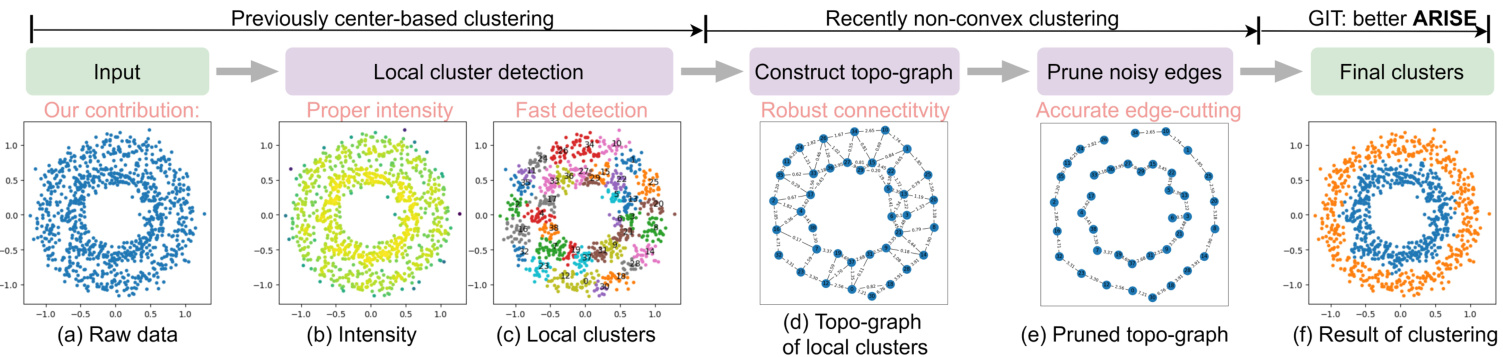
Figure 1: The pipeline of GIT: after the intensity function in (b) has been estimated from the raw data (two rings) in (a), local clusters (c) are detected through the intensity growing process, seeing Section. 2.3. Due to the limited number of colors, different local clusters may share the same color. (d) shows that each local cluster is represented as a vertex in the topological graph, and edges between them are calculated. In (e), noisy edges are pruned and the real global structure (two rings) is revealed. Finally, the clustering task is finished by merging connected local lusters, as shown in (f).
图 1: GIT流程示意图:(a)中原始数据(双环形结构)经过(b)强度函数估计后,通过第2.3节所述的强度增长过程检测出局部簇(c)。由于颜色数量有限,不同局部簇可能使用相同颜色标识。(d)展示每个局部簇被表示为拓扑图中的顶点,并计算它们之间的边连接。(e)经过噪声边剪枝后,真实的全局结构(双环形)得以显现。最终如(f)所示,通过合并相连的局部簇完成聚类任务。
In summary, we propose GIT to achieve better ARISE performance, considering both local and global data structures. Extensive experiments confirm this claim.
总之,我们提出GIT方法以同时兼顾局部和全局数据结构,从而实现更好的ARISE性能。大量实验证实了这一主张。
Table 1: Commonly used symbols
表 1: 常用符号
| 符号 | 描述 |
|---|---|
| D | 数据集,包含 c1, c2, ..., cn。 |
| n | 样本数量。 |
| k | 超参数,用于 kNN 搜索。 |
| ds | 输入特征维度数量。 |
| ri | 第 i 个局部簇的根(或强度峰值)。 |
| R(c) | 包含 c 的局部簇的根。 |
| R | 根点集合。 |
| S(·) | 局部簇之间的相似性。 |
| S(·,·) | 基于局部簇的样本间相似性。 |
| f(c) | c 的强度。 |
| L(λ) | 强度函数的超水平集,阈值为 λ。 |
| Ci(t) | 时间 t 的第 i 个局部簇。 |
2 Method
2 方法
2.1 Motivation, Symbols and Pipeline
2.1 动机、符号与流程
In Fig. 2, we illustrate the motivation that local clusters are point sets in high-intensity regions and they are connected by shared boundaries. And GIT aims to
在图 2 中,我们展示了局部簇作为高密度区域点集并通过共享边界连接的动机。GIT 的目标是
- determine local clusters via the intensity function; 2. construct the connectivity graph of local clusters; 3. cut noisy edges for reading out final clusters, each of which contains several connected local clusters.
- 通过强度函数确定局部聚类;
- 构建局部聚类的连通图;
- 切断噪声边以读取最终聚类,每个最终聚类包含多个相连的局部聚类。
The commonly used symbols and the overall pipeline are shown in Table. 1 and Fig. 1.
常用符号及整体流程如表 1 和图 1 所示。
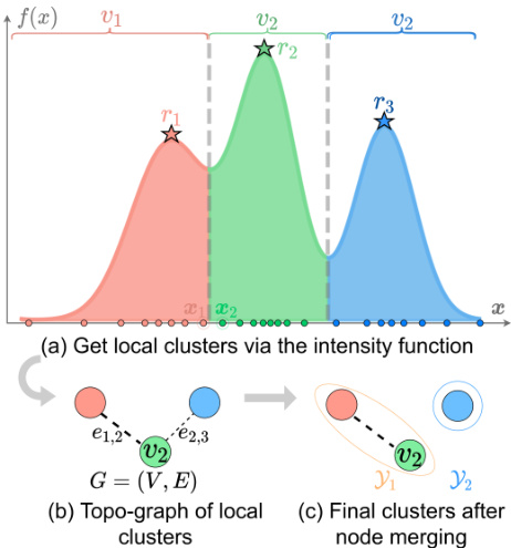
Figure 2: Motivation with 1D data. In (a), we estimate the intensity function $f(x)$ from samples and partition data into local clusters ${v_{1},v_{2},v_{3}}$ along valleys. Points with the largest intensity are called roots of local clusters, such as $r_{1},r_{2}$ and $r_{3}$ . $(\pmb{x}{1},\pmb{x}{2})$ is a boundary pair connecting $v_{1}$ and $v_{2}$ . (b) shows the topology graph containing local clusters (nodes) and their connectivity (edges), where $e_{1,2}$ is stronger than $^{\textstyle e_{2,3},}$ . In (c), by cutting $^{e_{2,3}}$ , we get final clusters $\mathcal{V}{1}={v_{1},v_{2}}$ and $\mathcal{V}{2}={v_{3}}$ .
图 2: 一维数据动机示意图。(a) 中我们从样本估计强度函数 $f(x)$ 并将数据沿谷值划分为局部聚类 ${v_{1},v_{2},v_{3}}$。强度最大的点称为局部聚类的根,例如 $r_{1},r_{2}$ 和 $r_{3}$。$(\pmb{x}{1},\pmb{x}{2})$ 是连接 $v_{1}$ 和 $v_{2}$ 的边界对。(b) 展示了包含局部聚类(节点)及其连接性(边)的拓扑图,其中 $e_{1,2}$ 的强度大于 $^{\textstyle e_{2,3},}$。(c) 中通过切断 $^{e_{2,3}}$,我们得到最终聚类 $\mathcal{V}{1}={v_{1},v_{2}}$ 和 $\mathcal{V}{2}={v_{3}}$。
2.2 Intensity Function
2.2 强度函数
To identify local clusters, non-parametric kernel density estimation (KDE) is employed to estimate the data distribution. However, the kernel-based (Parzen 1962; Davis, Lii, and Politis 2011) or $\mathbf{k}$ -Nearest Neighborhood(KNN)-based (Lofts ga arden, Que sen berry et al. 1965) KDE either suffers from global over-smoothing or local oscillator y (Yip, Ding, and Chan 2006), both of which are not suitable for GIT. Instead, we use a new intensity function $f(x)$ for better empirical performance:
为识别局部聚类,采用非参数核密度估计(KDE)来估算数据分布。然而基于核方法(Parzen 1962; Davis, Lii和Politis 2011)或k近邻(KNN)方法(Loftsgaarden, Quesenberry等1965)的KDE会面临全局过平滑或局部振荡问题(Yip, Ding和Chan 2006),这两种情况都不适用于GIT。为此,我们采用新的强度函数$f(x)$以获得更好的实证效果:
$$
f(\pmb{x})=\frac{1}{|\mathscr{N}{\pmb{x}}|}\sum_{\pmb{y}\in\mathscr{N}{\pmb{x}}}e^{-d(\pmb{x},\pmb{y})};d(\pmb{x},\pmb{y})=\sqrt{\sum_{j=1}^{s}\frac{(x_{j}-y_{j})^{2}}{\sigma_{j}^{2}}},
$$
$$
f(\pmb{x})=\frac{1}{|\mathscr{N}{\pmb{x}}|}\sum_{\pmb{y}\in\mathscr{N}{\pmb{x}}}e^{-d(\pmb{x},\pmb{y})};d(\pmb{x},\pmb{y})=\sqrt{\sum_{j=1}^{s}\frac{(x_{j}-y_{j})^{2}}{\sigma_{j}^{2}}},
$$
where $\mathcal{N}{x}$ is ${x}$ ’s neighbors for intensity estimation and $\sigma_{j}$ is the standard deviation of the $j$ -th dimension. With the consideration of $\sigma_{j}$ , $d(\cdot,\cdot)$ is robust to the absolute data scale. We estimate the intensity for each point in its neighborhood, avoiding the global over-smoothing. The exponent kernel is helpful to avoid local oscillator y, and we show that $f(x)$ is Lipschitz continuous under a mild condition, seeing Appendix. 5.1.
其中 $\mathcal{N}{x}$ 是 ${x}$ 的邻域用于强度估计,$\sigma_{j}$ 是第 $j$ 维的标准差。通过考虑 $\sigma_{j}$,$d(\cdot,\cdot)$ 对绝对数据尺度具有鲁棒性。我们为每个点在其邻域内估计强度,避免全局过度平滑。指数核有助于避免局部振荡,并且在温和条件下可以证明 $f(x)$ 是 Lipschitz 连续的,详见附录 5.1。
2.3 Local Clusters
2.3 本地集群
A local cluster is a set of points belonging to the same highintensity region. Once the intensity function is given, how to efficiently detect these local clusters is the key problem.
局部聚类是指属于同一高密度区域的一组点。在给定强度函数后,如何高效检测这些局部聚类成为关键问题。
We introduce a fast algorithm that collects points within the same intensity peak by searching along the gradient direction of the intensity function (refer to Fig. 8, Appendix. 5.1). Although similar approaches have been proposed before (Chazal et al. 2013; Rodriguez and Laio 2014), we provide comprehensive time complexity analysis and take connected boundary pairs (introduced in Section. 2.4) of adjacent local clusters into considerations. To clarify this approach, we formally define the root, gradient flow and $l o$ - cal clusters. Then we introduce a density growing process for an efficient algorithmic implementation.
我们提出了一种快速算法,该算法通过沿强度函数的梯度方向搜索来收集同一强度峰内的点(参见附录5.1中的图8)。尽管之前已有类似方法被提出(Chazal等人2013;Rodriguez和Laio 2014),但我们提供了全面的时间复杂度分析,并考虑了相邻局部簇的连通边界对(见第2.4节)。为阐明该方法,我们正式定义了根、梯度流和局部簇,随后介绍了一种高效算法实现的密度增长过程。
Definition. (root, gradient flow, local clusters) Given intensity function $f({\pmb x})$ , the set of roots is $\mathcal{R} = {r|\nabla f(r) = 0,|\nabla^{2}f(r)| < 0,r~\in~\mathcal{X}}$ , i.e., the local maximum. For any point $\textbf{\textit{x}}\in\mathbb{R}^{d_{s}}$ , there is a gradient flow $\pi_{\pmb{x}}:[0,1]\mapsto\mathbb{R}^{d_{s}}$ , starting at $\pi_{\pmb{x}}(0) =~\pmb{x}$ and ending in $\pi_{\pmb{x}}(1)\overset{}{=\i}R(\pmb{x})$ , where $R({\pmb x})\in\mathcal{R}$ . A local cluster a set of points converging to the same root along the gradient flow, e.g., ${\pmb{x}|R(\pmb{x})\in\mathcal{R},\pmb{x}\in\mathcal{X}}$ . To better understand, please see Fig. 8 in Appendix. 5.1.
定义。 (root, gradient flow, local clusters) 给定强度函数 $f({\pmb x})$,其根集为 $\mathcal{R} = {r|\nabla f(r) = 0,|\nabla^{2}f(r)| < 0,r~\in~\mathcal{X}}$,即局部最大值点。对于任意点 $\textbf{\textit{x}}\in\mathbb{R}^{d_{s}}$,存在一条梯度流 $\pi_{\pmb{x}}:[0,1]\mapsto\mathbb{R}^{d_{s}}$,起始于 $\pi_{\pmb{x}}(0) =~\pmb{x}$ 并终止于 $\pi_{\pmb{x}}(1)\overset{}{=\i}R(\pmb{x})$,其中 $R({\pmb x})\in\mathcal{R}$。局部簇是指沿梯度流收敛至同一根点的点集,即 ${\pmb{x}|R(\pmb{x})\in\mathcal{R},\pmb{x}\in\mathcal{X}}$。具体示意图参见附录5.1中的图8。
Intensity Growing Process. As shown in Fig. 3, points with higher intensities appear earlier and local clusters grow as the time goes on. We formally define the intensity growing process via a series of super-level sets w.r.t. $\lambda$ :
强度增长过程。如图 3 所示,强度较高的点出现较早,随着时间推移局部簇逐渐增长。我们通过一系列关于 $\lambda$ 的超水平集来正式定义强度增长过程:
$$
L_{\lambda}^{+}={{\pmb x}|f({\pmb x})\geq\lambda}.
$$
$$
L_{\lambda}^{+}={{\pmb x}|f({\pmb x})\geq\lambda}.
$$
We introduce a time variable $t,1\leq t\leq n$ , such that $\lambda_{t-1}\geq$ $\lambda_{t}$ . At time $t$ , the $i$ -th local cluster is
我们引入一个时间变量 $t,1\leq t\leq n$,使得 $\lambda_{t-1}\geq$ $\lambda_{t}$。在时间 $t$,第 $i$ 个本地聚类为
$$
C_{i}(t)={\pmb{x}|R(\pmb{x})=\pmb{r}{i},\pmb{x}\in L_{\lambda_{t}}^{+}},
$$
$$
C_{i}(t)={\pmb{x}|R(\pmb{x})=\pmb{r}{i},\pmb{x}\in L_{\lambda_{t}}^{+}},
$$
where $R(\cdot)$ is the root function, $\mathbf{\nabla}{\mathbf{\phi}}\mathbf{\mathit{r}}{i}$ is the $i$ -th root. It is obvious that $L_{\lambda_{t-1}}^{+}\subset L_{\lambda_{t}}^{+}$ and $L_{\lambda_{n}}^{+}=\chi$ . When $t=n$ , we can get all local clusters $C_{1}(n),C_{2}(n),...$ Next, we introduce a recursive function to efficiently compute $C_{i}(t)$ .
其中 $R(\cdot)$ 是根函数,$\mathbf{\nabla}{\mathbf{\phi}}\mathbf{\mathit{r}}{i}$ 是第 $i$ 个根。显然 $L_{\lambda_{t-1}}^{+}\subset L_{\lambda_{t}}^{+}$ 且 $L_{\lambda_{n}}^{+}=\chi$。当 $t=n$ 时,我们可以得到所有局部聚类 $C_{1}(n),C_{2}(n),...$。接下来,我们引入一个递归函数来高效计算 $C_{i}(t)$。
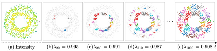
Figure 3: Example of the intensity growth process. (a) shows the estimated intensities; and (b), (c), (d), (e) show the growing process of local clusters as $\lambda_{t}$ gradually decays. We mark the unborn points in light gray and highlight local clusters. Limited by the number of colors, different local clusters may share the same color.
图 3: 强度增长过程示例。(a) 展示估计强度值;(b)、(c)、(d)、(e) 显示随着 $\lambda_{t}$ 逐渐衰减时局部簇的形成过程。未出生点标记为浅灰色,局部簇以高亮显示。受颜色数量限制,不同局部簇可能共用相同颜色。
Efficient Implementation. For each point $\scriptstyle{\boldsymbol{x}}{i}$ , to determine whether it creates a new local cluster or belongs to existing one, we need to compute its intensity2 and its parent point $P a(\pmb{x}{i})$ along the gradient direction. We determine $P a(\pmb{x}{i})$ as the neighbor which has maximum directional derivative from $\pmb{x}{i}$ to $P a(\pmb{x}_{i})$ , that is
高效实现。对于每个点 $\scriptstyle{\boldsymbol{x}}{i}$,为了确定它是创建新局部聚类还是属于现有聚类,我们需要计算其强度2及其沿梯度方向的父点 $P a(\pmb{x}{i})$。我们将 $P a(\pmb{x}{i})$ 确定为从 $\pmb{x}{i}$ 到 $P a(\pmb{x}_{i})$ 具有最大方向导数的邻居点,即
$$
P a(\pmb{x}{i})=\arg\operatorname*{max}{\pmb{x}{p}\in L_{f(\pmb{x}{i})}^{+}\cap\mathcal{N}{\pmb{x}{i}}}\frac{f(\pmb{x}{p})-f(\pmb{x}{i})}{||\pmb{x}{p}-\pmb{x}_{i}||},
$$
$$
P a(\pmb{x}{i})=\arg\operatorname*{max}{\pmb{x}{p}\in L_{f(\pmb{x}{i})}^{+}\cap\mathcal{N}{\pmb{x}{i}}}\frac{f(\pmb{x}{p})-f(\pmb{x}{i})}{||\pmb{x}{p}-\pmb{x}_{i}||},
$$
where $i=1,2,\ldots,n_{t-1}{}^{3}$ . Eq. 6 means that 1) if $\scriptstyle{\boldsymbol{x}}{i}$ ’s father is itself, $\boldsymbol{\mathbf{\mathit{x}}}{i}$ is the peak point and creates a new local cluster ${\pmb{x}{i}}$ , 2) if $\scriptstyle{\boldsymbol{x}}{i}$ ’s father shares the same root with $C_{i}(t-1)$ , $\scriptstyle{\boldsymbol{x}}{i}$ will be absorbed by $C_{i}(t-1)$ to generate $C_{i}(t)$ , and 3) local clusters which is irrelevant to $\scriptstyle{\boldsymbol{x}}{i}$ remain unchanged. We treat $R(\cdot)$ as a mapping table and update it on-the-fly. $C_{i}(t)$ is obviously recursive (Davis 2013). The time complexity of computing $C_{i}(n)$ is $\mathcal{O}(n\times\mathrm{cost}(P a))^{4}$ , where $\mathsf{c o s t}(P a)$ is $\mathcal{O}(k d_{s}\log n)$ for querying $k$ neighbors.
其中 $i=1,2,\ldots,n_{t-1}{}^{3}$。式6表示:1) 若 $\scriptstyle{\boldsymbol{x}}{i}$ 的父节点是其自身,则 $\boldsymbol{\mathbf{\mathit{x}}}{i}$ 为峰值点并创建新局部聚类 ${\pmb{x}{i}}$;2) 若 $\scriptstyle{\boldsymbol{x}}{i}$ 的父节点与 $C_{i}(t-1)$ 同根,则 $\scriptstyle{\boldsymbol{x}}{i}$ 将被 $C_{i}(t-1)$ 吸收生成 $C_{i}(t)$;3) 与 $\scriptstyle{\boldsymbol{x}}{i}$ 无关的局部聚类保持不变。我们将 $R(\cdot)$ 视为映射表并实时更新。显然 $C_{i}(t)$ 具有递归性 (Davis 2013)。计算 $C_{i}(n)$ 的时间复杂度为 $\mathcal{O}(n\times\mathrm{cost}(P a))^{4}$,其中 $\mathsf{c o s t}(P a)$ 为查询 $k$ 近邻的 $\mathcal{O}(k d_{s}\log n)$。
In summary, by applying Eq. 4-7, we can obtain local clusters $C_{1}\dot{(}n),\dot{C}{2}\dot{(}n),\cdot\cdot\cdot$ with time complexity $\mathscr{O}(d_{s}n\log n)$ . For simplicity, we write $C_{i}(n)$ as $C_{i}$ in later sections. The detailed local cluster detection algorithm 1 can be found in the Appendix.
总之,通过应用公式4-7,我们可以在时间复杂度$\mathscr{O}(d_{s}n\log n)$下获得局部聚类$C_{1}\dot{(}n),\dot{C}{2}\dot{(}n),\cdot\cdot\cdot$。为简化表述,后文将$C_{i}(n)$记为$C_{i}$。详细的局部聚类检测算法1见附录。
2.4 Construct Topo-graph
2.4 构建拓扑图
Instead of using local clusters as final results (Comaniciu and Meer 2002; Chazal et al. 2013; Rodriguez and Laio 2014; Jiang, Jang, and Kpotufe 2018), we further consider connect iv i ties between them for improving the results. For example, local clusters that belong to the same class usually have stronger connect iv i ties. Meanwhile, there is a risk that noisy connect iv i ties may damage performance. We manage local clusters and their connect iv i ties with a graph, namely topo-graph, and the essential problem is cutting noisy edges.
我们并未将局部聚类作为最终结果 (Comaniciu and Meer 2002; Chazal et al. 2013; Rodriguez and Laio 2014; Jiang, Jang, and Kpotufe 2018),而是进一步考虑它们之间的连接性以优化结果。例如,属于同一类别的局部聚类通常具有更强的连接性。然而,噪声连接可能损害性能。我们通过图结构(即拓扑图)管理局部聚类及其连接性,核心问题在于剔除噪声边。
Connectivity. According to UPGMA standing for unweighted pair group method using arithmetic averages (Jain and Dubes 1988; Gan, Ma, and Wu 2020), the similarity $S(\cdot,\cdot)$ between $C_{i},C_{j}\cup C_{k}$ can be obtained from the LanceWilliams formula:
连通性。根据代表算术平均非加权配对组方法的UPGMA (Jain and Dubes 1988; Gan, Ma, and Wu 2020),$C_{i},C_{j}\cup C_{k}$之间的相似度$S(\cdot,\cdot)$可通过LanceWilliams公式获得:
$$
\begin{array}{l}{{S(C_{i},C_{j}\cup C_{k})=}}\ {{\displaystyle\frac{|C_{j}|}{|C_{j}|+|C_{k}|}S(C_{i},C_{j})+\frac{|C_{k}|}{|C_{j}|+|C_{k}|}S(C_{i},C_{k}),}}\end{array}
$$
$$
\begin{array}{l}{{S(C_{i},C_{j}\cup C_{k})=}}\ {{\displaystyle\frac{|C_{j}|}{|C_{j}|+|C_{k}|}S(C_{i},C_{j})+\frac{|C_{k}|}{|C_{j}|+|C_{k}|}S(C_{i},C_{k}),}}\end{array}
$$
and
和
$$
S(C_{i},C_{j})=\frac{1}{|C_{i}||C_{j}|}\sum_{{\pmb x}\in C_{i},{\pmb y}\in C_{j}}s_{l}({\pmb x},{\pmb y}),
$$
$$
S(C_{i},C_{j})=\frac{1}{|C_{i}||C_{j}|}\sum_{{\pmb x}\in C_{i},{\pmb y}\in C_{j}}s_{l}({\pmb x},{\pmb y}),
$$
Note that $s_{l}({\pmb x},{\pmb y})$ is non-zero only if ${x}$ and $\textit{\textbf{y}}$ are mutual neighborhood and belong to different local clusters, in which case $(x,y)$ is a boundary pair of adjacent local clusters, e.g., ${x_{1}}$ and $\mathbf{\delta}{\mathbf{\delta}{x_{2}}}$ in Fig. 2. Fortunately, all the boundary pairs among local clusters can be obtained from previous intensity growing process, without further computation.
注意,$s_{l}({\pmb x},{\pmb y})$ 仅在 ${x}$ 和 $\textit{\textbf{y}}$ 互为邻域且属于不同局部聚类时非零,此时 $(x,y)$ 是相邻局部聚类的边界对,例如图 2 中的 ${x{1}}$ 和 $\mathbf{\delta}{\mathbf{\delta}{x_{2}}}$。幸运的是,所有局部聚类间的边界对都可以通过先前的强度增长过程获得,无需额外计算。
Topo-graph. We construct the topo-graph as $G=(V,E)$ , where $v_{i}$ is the $i$ -th local cluster $C_{i}$ and $e_{i,j}=S(C_{i},C_{j})$ .
拓扑图 (Topo-graph)。我们将拓扑图构建为 $G=(V,E)$,其中 $v_{i}$ 表示第 $i$ 个局部聚类 $C_{i}$,$e_{i,j}=S(C_{i},C_{j})$。
In summary, we introduce a well-defined connectivity between local clusters using connected boundary pairs. The detailed topo-graph construction algorithm 3 can be found in the Appendix, whose time complexity is $\mathcal{O}(k n)$ .
总之,我们通过连接边界对在局部聚类之间建立了明确的连通性。详细的拓扑图构建算法3可在附录中找到,其时间复杂度为 $\mathcal{O}(k n)$。
2.5 Edges Cutting and Final Clusters
2.5 边缘切割与最终聚类
To capture global data structures, connected local clusters are merged as final clusters, as shown in Fig. 1(e, f). However, the original topo-graph is usually dense, indicating redundant (or noisy) edges which lead to trivial solutions, e.g., all the local clusters are connected, and there is one final cluster. In this case, cutting noisy edges is necessary and the simplest way is to set a threshold to filter weak edges or using spectral clustering. However, we find that these methods are either sensitive, hard to tune or inaccurate, which severely limits the widely usage of similar approaches. Is there a robust and accurate way to filter noisy edges using available prior knowledge?
为捕捉全局数据结构,相连的局部聚类会被合并为最终聚类,如图1(e, f)所示。然而原始拓扑图通常较为稠密,存在冗余(或噪声)边,这会导致平凡解,例如所有局部聚类相连而仅形成一个最终聚类。此时需剪除噪声边,最简单的方法是设定阈值过滤弱边或使用谱聚类。但我们发现这些方法要么敏感难调参,要么精度不足,严重制约了同类方法的广泛应用。是否存在利用现有先验知识过滤噪声边的鲁棒且准确的方法?
Auto Edge Filtering. To make GIT more easy to use and accurate, we automatically filter edges with the help of pior class proportion. Firstly, we define a metric about final clusters by comparing the predicted and pior proportions, such that the higher the proportion score, the better the result (seeing the next paragraph). We sort edges with connectivity strengths from high to low, in which order we merge two end local clusters for each edge if this operation gets a higher score. In this process, edges that cannot increase the metric score are regarded as noisy edges and will be cutted.
自动边缘过滤。为使GIT更易用且精准,我们借助先验类别比例自动过滤边缘。首先,通过比较预测比例与先验比例定义最终聚类的评估指标(比例分数越高结果越优,详见下段)。按连接强度从高到低排序边缘,依次合并两端局部聚类(当该操作能提高分数时)。在此过程中,无法提升指标分数的边缘被视为噪声边缘并被切除。
Metric about Final Clusters. Let $\pmb{p}=[p_{1},p_{2},\dots,p_{m}]$ and $\pmb q=[q_{1},q_{2},\dots,q_{m^{\prime}}]$ be predicted and predefined class proportions, where $\begin{array}{r}{\sum_{i=1}^{m}p_{i}=1,\sum_{i}^{m^{\prime}}q_{i}=1}\end{array}$ . We take the similarity between ${p}$ and $\pmb q$ as t he aforementioned metric score. Because $m$ and $m^{\prime}$ may not be equal and the order of elements in $_{p}$ and $\pmb q$ is random, it is not feasible to use conventional Lp-norm. Instead, we use Wasser stein Distance to measure the similarity and define the metric $\mathcal{M}(\pmb{p},\pmb{q})$ as:
关于最终聚类的度量。令 $\pmb{p}=[p_{1},p_{2},\dots,p_{m}]$ 和 $\pmb q=[q_{1},q_{2},\dots,q_{m^{\prime}}]$ 分别表示预测和预定义的类别比例,其中 $\begin{array}{r}{\sum_{i=1}^{m}p_{i}=1,\sum_{i}^{m^{\prime}}q_{i}=1}\end{array}$。我们将 $\pmb{p}$ 与 $\pmb q$ 之间的相似度作为前述度量得分。由于 $m$ 和 $m^{\prime}$ 可能不相等,且 $\pmb{p}$ 和 $\pmb q$ 中元素的顺序是随机的,使用传统的 Lp 范数不可行。因此,我们采用 Wasserstein 距离来衡量相似性,并将度量 $\mathcal{M}(\pmb{p},\pmb{q})$ 定义为:
$$
\begin{array}{l}{{\mathcal{M}}({\pmb{p}},{\pmb q})=\mathrm{Exp}(-\underset{\gamma_{i,j}\geq0}{m i n}\displaystyle\sum_{i,j}\gamma_{i,j})}\ {{s.t.\qquad\displaystyle\sum_{j}\gamma_{i,j}=p_{i};\quad\displaystyle\sum_{i}\gamma_{i,j}=q_{j},}}\end{array}
$$
$$
\begin{array}{l}{{\mathcal{M}}({\pmb{p}},{\pmb q})=\mathrm{Exp}(-\underset{\gamma_{i,j}\geq0}{m i n}\displaystyle\sum_{i,j}\gamma_{i,j})}\ {{s.t.\qquad\displaystyle\sum_{j}\gamma_{i,j}=p_{i};\quad\displaystyle\sum_{i}\gamma_{i,j}=q_{j},}}\end{array}
$$
where the original Wasser stein Distance is $\begin{array}{r}{m i n\sum_{i,j}\gamma_{i,j}d_{i,j},\tilde{\gamma}{i,j}}\ {\gamma_{i,j}\geq0\sum_{i,j}\gamma_{i,j}d_{i,j},}\end{array}$ is the trans pot ation cost from $i$ to $j$ , and we set $d_{i,j}=1$ . Because $\dim(p_{i})=\dim(q_{j})=1$ , Eq. 11 can be efficiently calculated by linear programming.
原始Wasserstein距离为 $\begin{array}{r}{m i n\sum_{i,j}\gamma_{i,j}d_{i,j},\tilde{\gamma}{i,j}}\ {\gamma_{i,j}\geq0\sum_{i,j}\gamma_{i,j}d_{i,j},}\end{array}$ ,其中 $d_{i,j}$ 表示从 $i$ 到 $j$ 的传输成本,我们设 $d_{i,j}=1$ 。由于 $\dim(p_{i})=\dim(q_{j})=1$ ,公式11可通过线性规划高效计算。
In summary, we introduce a new metric of class proportion and use it to guide the process of edge filtering, then merge connected local clusters as final clusters. Compared to threshold-based or spectral-based edge cutting, this algorithm considers available prior knowledge to reduce the difficulty of parameter tuning or provide higher accuracy. By default, we set the same proportion for each category if only the number of classes is known. Besides, it is promising for dealing with sample imbalances if we know the actual proportion, seeing Section. 3.1 for ex peri metal evidence.
总结来说,我们引入了一种新的类别比例度量指标,并利用其指导边缘过滤过程,最终将连通的局部聚类合并为最终聚类。与基于阈值或谱分析的边缘切割方法相比,该算法通过整合先验知识来降低参数调优难度或提供更高精度。默认情况下,若仅已知类别数量,我们会为每个类别设置相同比例。此外,若已知实际类别分布比例,该方法在处理样本不平衡问题时表现优异 (详见第3.1节实验验证)。
3 Experiments
3 实验
In this section, we conduct experiments on a series of synthetic, small-scale and large-scale datasets to study the Accuracy, Robustness to shapes, noises and scales, Speed and Easy to use, while the Interpret ability of GIT has been demonstrated in previous sections. As an extension, we further investigate how PCA and AE (auto encoder) work with GIT to further improve the accuracy.
在本节中,我们通过一系列合成数据集、小规模和大规模数据集进行实验,研究GIT在准确度、对形状/噪声/尺度的鲁棒性、速度及易用性方面的表现(其可解释性已在前面章节得到验证)。作为扩展,我们进一步探究PCA和AE(auto encoder)如何与GIT协同工作以提升准确度。
Baselines. GIT is compared to density-based methods, such as FSFDP (Rodriguez and Laio 2014), HDBSCAN (McInnes and Healy 2017), Quickshift $^{++}$ (Jiang, Jang, and
基线方法。GIT与基于密度的方法进行比较,例如FSFDP (Rodriguez and Laio 2014)、HDBSCAN (McInnes and Healy 2017)、Quickshift$^{++}$ (Jiang, Jang和
Kpotufe 2018), SpectACl (Hess et al. 2019) and DPA (d’Errico et al. 2021). Besides, classical Spectral Clustering and $k$ -means $^{++}$ (Pedregosa et al. $201\bar{1})^{5}$ . Since there is little work comprehensively comparing recent clustering algorithms, our results can provide a reliable baseline for subsequent researches. For simplicity, we use these abbreviations: FSF (FSFDP), HDB (HDBSCAN), QSP (QuickshiftPP), SA (SpectACI), DPA (DPA), SC (Spectral Clustering) and KM ( $k$ -means $++$ ).
Kpotufe 2018)、SpectACl (Hess et al. 2019) 和 DPA (d'Errico et al. 2021)。此外还包括经典谱聚类和 $k$-means$^{++}$ (Pedregosa et al. $201\bar{1})^{5}$。由于目前缺乏对近期聚类算法的全面比较研究,我们的结果可为后续研究提供可靠基线。为简洁起见,我们使用以下缩写:FSF (FSFDP)、HDB (HDBSCAN)、QSP (QuickshiftPP)、SA (SpectACI)、DPA (DPA)、SC (谱聚类) 和 KM ($k$-means$++$)。
Metrics. We report F1-score (Evett and Spiehler 1999), Adjusted Rand Index (ARI) (Hubert and Arabie 1985) and Normalized Mutual Information (NMI) (Vinh, Epps, and Bailey 2010) to measure the clustering results. F1-score evaluates both each class’s accuracy and the bias of the model, ranging from 0 to 1. ARI is a measure of agreement between partitions, ranging from $-1$ to 1, and if it is less than 0, the model does not work in the task. NMI is a normalization of the Mutual Information (MI) score, where the result is scaled to range of 0 (no mutual information) and 1 (perfect correlation). Besides, because HDBSCAN and DPA perfer to drop some valid points as noises, we also consider the fraction of samples assigned to clusters, namely cover rate. If the cover rate is less than 0.8, we will ignore this result and mark it in gray. The math mat ical formulas of these metrics can be found in the Appendix. 5.2. For each methods, we carefully tune the hyper parameters (which can be found in the open-source code), and report the best results.
指标。我们采用F1分数 (Evett and Spiehler 1999)、调整兰德指数(ARI) (Hubert and Arabie 1985)和标准化互信息(NMI) (Vinh, Epps, and Bailey 2010)来评估聚类结果。F1分数同时衡量每个类别的准确率和模型偏差,取值范围为0到1。ARI用于衡量分区间一致性,取值范围为$-1$到1,若小于0则表明模型在该任务中失效。NMI是互信息(MI)得分的归一化结果,其值域为0(无互信息)到1(完全相关)。此外,由于HDBSCAN和DPA倾向于将部分有效点标记为噪声,我们还考虑了被分配到簇的样本比例(即覆盖率)。若覆盖率低于0.8,我们将忽略该结果并以灰色标注。这些指标的数学公式详见附录5.2。针对每种方法,我们精细调整了超参数(详见开源代码),并报告最佳结果。
Datasets. We evaluate algorithms on synthetic, smallscale and large-scale datasets. In Table. 2, we count the number of samples, feature dimensions, number of classes and balance rate for real-world datasets. The balance rate is the sample ratio of the smallest calss to the largest class. All these datasets are available online (Asuncion and Newman 2007; Deng 2012; Xiao, Rasul, and Vollgraf 2017).
数据集。我们在合成数据集、小规模数据集和大规模数据集上评估算法性能。表2统计了真实数据集的样本数量、特征维度、类别数量及平衡率(样本最小类与最大类的数量比值)。所有数据集均来自公开资源 (Asuncion and Newman 2007; Deng 2012; Xiao, Rasul, and Vollgraf 2017)。
Table 2: Statistics of real-world datasets.
表 2: 真实世界数据集统计
| dataset | #samples | #dim | #class | balancerate | |
|---|---|---|---|---|---|
| sm | Iris | 150 | 4 | 3 | 1.00 |
| Wine | 178 | 13 | 3 | 0.68 | |
| Hepatitis | 154 | 19 | 2 | 0.26 | |
| Cancer | 569 | 30 | 2 | 0.59 | |
| Olivettiface | 400 | 4096 | 40 | 1.00 | |
| lar 50 | MNIST | 60000 | 784 | 10 | 1.00 |
| FMNIST | 60000 | 784 | 10 | 1.00 | |
| Frogs | 7195 | 22 | 10 | 0.02 | |
| Codon | 13028 | 24 | 11 | 0.01 | |
Platform. The platform for our experiment is ubuntu 18.04, with a AMD Ryzen Thread ripper 3970X 32-Core cpu and 256GB memory. We fairly compare all algorithms on this platform for research convenience.
平台。我们的实验平台为 Ubuntu 18.04 系统,配备 AMD Ryzen Threadripper 3970X 32 核 CPU 和 256GB 内存。为便于研究,我们在该平台上对所有算法进行了公平比较。
3.1 Accuracy
3.1 准确度
Objective and Setting. To study the accuracy of various algorithms, we: 1) firstly compare GIT with density-based FSF, HDB, QSP, SA, and DPA on small-scale datasets to determine their priority order, 2) and secondly choose the top-3 (F1-score) density-based algorithms and $k$ -means $^{++}$ as baselines to further compare with GIT on large-scale datasets. With the exception of Frogs and Codon, which are extremely unbalanced, all the class proportions are set to be the same in GIT, e.g. 1:1:1 for three classes.
目标与设定。为研究不同算法的准确性,我们:1) 首先在小规模数据集上比较GIT与基于密度的FSF、HDB、QSP、SA及DPA算法以确定优先级顺序;2) 随后选取F1分数前三的基于密度算法和 $k$ -means $^{++}$ 作为基线,在大规模数据集上与GIT进一步对比。除极度不平衡的Frogs和Codon数据集外,GIT中所有类别比例均设为相同(例如三分类为1:1:1)。
Result and Analysis. Comparisons on small-scale and large-scale datasets are shown in Table. 3 and Table. 4. We notice that GIT outperforms other approaches, with the top3 ARI, top-2 NMI and top-1 F1-score in all cases. GIT also exceeds competitors up to $6%$ and $8%$ F1-score in the highly unbalanced case (Frogs and Condon) by specifying the actual prior class proportions. In addition, we find that the performance gains from GIT seem to be negatively correlated with the feature dimension, indicating the potential dimension curse. And we will introduce how to mitigate this problem through dimension reduction in Section. 3.5. Finally, the runtime of GIT is acceptable, especially on large scale datasets, where GIT is much faster than recent density-based clustering methods, such as HDB, QSP and SA.
结果与分析。小规模和大规模数据集上的比较结果如表 3 和表 4 所示。我们注意到 GIT 在所有情况下均优于其他方法,ARI 排名前三、NMI 排名前二、F1 分数排名第一。在高度不平衡的数据集(Frogs 和 Condon)中,通过指定实际先验类别比例,GIT 的 F1 分数最高可超出竞争对手 $6%$ 和 $8%$。此外,我们发现 GIT 的性能提升似乎与特征维度呈负相关,这表明可能存在维度诅咒问题。我们将在第 3.5 节介绍如何通过降维缓解该问题。最后,GIT 的运行时间是可接受的,尤其是在大规模数据集上,其速度远快于最近的基于密度的聚类方法(如 HDB、QSP 和 SA)。
Table 3: GIT vs density-based algorithms on small-scale datasets. The best and sub-optimum results are highlighted in bold and underline, respectively. Gray results are ignored because their cover rate is less than 0.8.
表 3: GIT与基于密度的算法在小规模数据集上的对比。最佳和次优结果分别用加粗和下划线标出。灰色结果因覆盖率低于0.8被忽略。
| DPA | FSF | HDB | QSP | SA | GIT | ||
|---|---|---|---|---|---|---|---|
| Iris | F1-score | 0.83 | 0.56 | 0.57 | 0.80 | 0.78 | 0.88 |
| ARI | 0.57 | 0.57 | 0.58 | 0.56 | 0.56 | 0.71 | |
| NMI | 0.68 | 0.73 | 0.74 | 0.58 | 0.63 | 0.76 | |
| Wine | F1-score | 0.38 | 0.62 | 0.54 | 0.73 | 0.70 | 0.90 |
| ARI | 0.05 | 0.31 | 0.30 | 0.39 | 0.36 | 0.71 | |
| NMI | 0.15 | 0.38 | 0.42 | 0.44 | 0.36 | 0.76 | |
| F1-score | 0.42 | 0.77 | 0.71 | 0.71 | 0.72 | 0.78 | |
| ARI | -0.05 | 0.50 | 0.05 | 0.02 | 0.06 | 0.23 | |
| NMI | 0.14 | 0.46 | 0.02 | 0.00 | 0.01 | 0.12 | |
| cane | F1-score | 0.70 | 0.72 | 0.78 | 0.78 | 0.92 | 0.93 |
| ARI | 0.00 | 0.00 | 0.40 | 0.41 | 0.69 | 0.73 | |
| NMI | 0.00 | 0.00 | 0.34 | 0.34 | 0.57 | 0.65 |
3.2 Easy to Use
3.2 易于使用
We introduce some experience for parameter tuning and auxiliary tool for data structure analysis.
我们介绍一些参数调优经验及数据结构分析的辅助工具。
Parameters Settings. Apart from the prior class proportion, there is only one hyper-parameter $k$ in GIT for kNN searching, which is usually less than 100. On large-scale datasets, we choose $k$ from $[30,40,50,60,70,80,90,100]$ . When only the number of classes is known, simply setting the ratio of all classes to be the same can generally yield good results. We admit that GIT cannot determine the number of classes from scratch and leave it for future work. If the actual proportion is known, GIT can obtain better results, even in highly unbalanced classes, seeing Frogs and Codon in Table. 4.
参数设置。除先验类别比例外,GIT中仅有一个用于kNN搜索的超参数$k$(通常小于100)。在大规模数据集上,我们从$[30,40,50,60,70,80,90,100]$中选取$k$值。当仅已知类别数量时,简单设置所有类别比例相同通常可获得良好效果。我们承认GIT无法从头推断类别数量,该问题将留待未来研究。若已知实际比例,即使如表4中Frogs和Codon的高度不平衡类别,GIT仍能获得更优结果。
Table 4: GIT vs SOTA algorithms on large-scale datasets.
表 4: GIT 与 SOTA 算法在大规模数据集上的对比
| KM | SC | HDB | QSP | SA | GIT | ||
|---|---|---|---|---|---|---|---|
| F1-score | 0.52 | 0.37 | 0.34 | 0.60 | 0.34 | 0.62 | |
| Face | ARI | 0.38 | 0.19 | 0.08 | 0.38 | 0.21 | 0.45 |
| NMI | 0.74 | 0.66 | 0.61 | 0.79 | 0.61 | 0.78 | |
| time | 2.6s | 0.4s | 0.9s | 0.8s | 1.1s | 2.1s | |
| F1-score | 0.50 | 0.41 | 0.99 | 0.45 | 0.40 | 0.59 | |
| MNIST | ARI | 0.36 | 0.33 | 0.99 | 0.13 | 0.17 | 0.42 |
| NMI | 0.45 | 0.44 | 0.99 | 0.45 | 0.33 | 0.53 | |
| time | 76.7s | 407.7s | 2037.0s | 3384.0s | 4096s | 422.1s | |
| FMNIST | F1-score | 0.39 | 0.43 | 0.06 | 0.42 | 0.47 | 0.56 |
| ARI | 0.35 | 0.34 | 0.01 | 0.16 | 0.29 | 0.32 | |
| NMI | 0.51 | 0.49 | 0.07 | 0.41 | 0.45 | 0.51 | |
| time | 54.6s | 397.7s | 1647.9s | 3832.6s | 4684s | 444.5s | |
| Frogs | F1-score | 0.47 | 0.60 | 0.95 | 0.50 | 0.60 | 0.66 |
| ARI | 0.40 | 0.41 | 0.96 | 0.21 | 0.49 | 0.69 | |
| NMI | 0.61 | 0.60 | 0.93 | 0.45 | 0.45 | 0.66 | |
| time | 0.18s | 3.7s | 1.2s | 0.5s | 2.9s | 3.2s | |
| Codon | F1-score | 0.25 | 0.37 | 0.21 | 0.24 | 0.19 | 0.45 |
| ARI | 0.19 | 0.24 | 0.05 | 0.04 | 0.02 | 0.31 | |
| NMI | 0.33 | 0.37 | 0.24 | 0.21 | 0.02 | 0.39 | |
| time | 1.1s | 11.6s | 10.2s | 7.9s | 82s | 16s |
Topo-graph Visualization. The topo-graph describes the global structure of the dataset, and GIT uses it to discover final clusters. We also provide API for users to visualize these topo-graphs to understand the inner structure better (d’Errico et al. 2021). One of the example of topo-graph can be found in Fig. 1(e).
拓扑图可视化。拓扑图描述了数据集的全局结构,GIT利用它来发现最终聚类。我们还为用户提供API以可视化这些拓扑图,从而更好地理解内部结构 (d'Errico et al. 2021)。图1(e)展示了一个拓扑图示例。
3.3 Speed
3.3 速度
Objective and Setting. To study the s cal ability of GIT, we generate artificial data from the mixture of two Gaussian with class proportion 1:1. We examine how dimension $(d_{s})$ , sample number $(n)$ and hyper-parameter $(k)$ affect the runtime, where $n\in[10^{4},10^{6}]$ , $\hat{d}{s}\in[10,10^{3}]$ and $k\in[10,10^{2}]$ . By default, $d_{s}=10,n=10^{4}$ and $k=50$ .
目标与设置。为研究GIT的可扩展性,我们通过混合两个高斯分布生成人工数据,类别比例为1:1。考察维度 $(d_{s})$ 、样本量 $(n)$ 和超参数 $(k)$ 对运行时间的影响,其中 $n\in[10^{4},10^{6}]$ , $\hat{d}{s}\in[10,10^{3}]$ , $k\in[10,10^{2}]$ 。默认参数为 $d_{s}=10,n=10^{4}$ 和 $k=50$ 。
Result and Analysis. The runtime impact of $n,d_{s}$ and $k$ is shown in Fig. 4. According to previous analysis, the time complexity of GIT is $O(d_{s}n\log n)$ , which is indeed confirmed by the experimental results. Since $k$ is limited within 100, seeing Section. 3.2, its effect on time complexity can be treated as a constant.
结果与分析。$n,d_{s}$ 和 $k$ 对运行时间的影响如图 4 所示。根据先前分析,GIT 的时间复杂度为 $O(d_{s}n\log n)$,实验结果确实验证了这一点。由于 $k$ 被限制在 100 以内(见第 3.2 节),其对时间复杂度的影响可视为常数。

Figure 4: The actual running time when changing sample number $(n)$ , feature dimension $(d_{s}$ )and hyper-parameter $(k)$ .
图 4: 改变样本数量 $(n)$ 、特征维度 $(d_{s})$ 和超参数 $(k)$ 时的实际运行时间。
3.4 Robustness
3.4 鲁棒性
Objective and Setting. To study the robustness to shapes, noises and scales of various algorithms, we: 1) firstly compare all algorithms on synthetic datasets with complex shapes, such as Circles and Moons, and show the top-3 (F1- score) results, 2) secondly compare GIT with top-3 competitors on Moons (with Gaussian noise) and Impossible (with Uniform noises), and 3) thirdly evaluate these methods under the mixed multi-scale data, e.g. a new dataset containing original cricles and enlarged circles in Fig. 6. We report F1- scores on different noise or scaling levels in Fig. 5.
目标与设置。为研究不同算法对形状、噪声和尺度的鲁棒性,我们:1) 首先在具有复杂形状的合成数据集(如 Circles 和 Moons)上比较所有算法,并展示前三名(F1分数)结果;2) 其次在添加高斯噪声的 Moons 数据集和均匀噪声的 Impossible 数据集上比较 GIT 与前三名竞争算法;3) 最后评估这些方法在混合多尺度数据下的表现,例如图 6 中同时包含原始圆形和放大圆形的新数据集。不同噪声或缩放级别下的 F1 分数结果如图 5 所示。
Table 5: Top-3 (F1-score) results on synthetic datasets with complex shapes. The first column is the ground truth data. Other columns show the clustering results from top-1 to top-3. We mark the corresponding method abbreviation under each result.
表 5: 复杂形状合成数据集上的Top-3 (F1分数) 结果。第一列为真实数据,其他列展示从top-1到top-3的聚类结果。我们在每个结果下方标注了对应的方法缩写。
| Data | Top1 | Top2 | Top3 |
|---|---|---|---|
| Circles | GIT | SA | QSP |
| Moons | GIT,QSP,SA | HDB | FSF |
| Impossible S-sets | GIT | HDB | QSP |
Result and Analysis. For shapes, we evaluate all baselines but only visualize the top-3 results in Table. 5. GIT is the best one to get the resonable clusters on all synthetic datasets and sup-optimum methods are SA, QSP, HDB and SC in turns. As expected, many baseline methods cannot deal with complex distributions (e.g., the Impossible dataset) for the lack of ability to identify global data structures, while GIT handles it well. For noises and scales, we compare GIT with SA and QSP in Table. 6, from which we find that GIT is more robust against noise and data scales, whereas SA and QSP both fail. What’s more, we plot the F1-scores of GIT, SA, QSP and HDB under different noise levels and scaling factors (Fig. 5), where GIT achieve the highest F1-score with smallest variance on the extreme situations. We believe the robustness comes from two aspects: On the one hand, the well-designed intensity function helps handle the multiscale issue because the kNN is invariant to scales, as proved in the Appendix (Theorem 1). On the other hand, the local and global clustering mechanism is helpful to anti-noise. Firstly, the process of local clustering detection is reliable because noises usually have a limited effect on the relative point intensities. Secondly, connectivity strength between two local clusters is also robust because it depends on all the adjacent boundary points, not just a few noisy points. As both nodes and edges of the topo-graph are robust to noise, the clustering results are undoubtedly robust.
结果与分析。对于形状数据集,我们评估了所有基线方法,但仅在表5中展示前3名的结果。GIT在所有合成数据集上都能获得合理的聚类效果,表现最优,其次是SA、QSP、HDB和SC。正如预期,许多基线方法由于缺乏识别全局数据结构的能力,无法处理复杂分布(例如Impossible数据集),而GIT则表现良好。对于噪声和尺度问题,我们在表6中比较了GIT、SA和QSP,发现GIT对噪声和数据尺度更具鲁棒性,而SA和QSP均失效。此外,我们绘制了GIT、SA、QSP和HDB在不同噪声水平和缩放因子下的F1分数(图5),其中GIT在极端情况下取得了最高的F1分数且方差最小。我们认为这种鲁棒性源于两个方面:一方面,精心设计的强度函数有助于处理多尺度问题,因为kNN对尺度具有不变性(附录中的定理1已证明);另一方面,局部和全局聚类机制有助于抗噪声。首先,局部聚类检测过程是可靠的,因为噪声对点的相对强度影响有限;其次,两个局部聚类之间的连接强度也具有鲁棒性,因为它依赖于所有相邻边界点,而非少数噪声点。由于拓扑图的节点和边都对噪声具有鲁棒性,聚类结果自然也具有鲁棒性。

Table 6: Comparing GIT with SA and QSP on noisy and multiscale datasets. The first column is the raw data and others are results of GIT, SA and QSP. We add 0.2 Gaussian noise on Circles, 0.1 Uniform noise on Impossible and mix two Circles as the multiscale data, where one Circles is 100 times larger than the other.
表 6: 在噪声和多尺度数据集上对比 GIT、SA 和 QSP 的效果。第一列为原始数据,其余列分别为 GIT、SA 和 QSP 的处理结果。我们在 Circles 数据集上添加了 0.2 的高斯噪声,在 Impossible 数据集上添加了 0.1 的均匀噪声,并将两个大小相差 100 倍的 Circles 数据集混合作为多尺度数据。

Figure 5: Performance comparison under different noise levels and scales. In (a), we change the (Gaussian) noise on Moons from 0.02 to 0.26 with step 0.02, and plot the average F1-score and its variance over 10 random seeds. In (b), we show the F1-score for each scaling factor ranging from 1 to 100 on the mixed Circles.
图 5: 不同噪声水平和尺度下的性能对比。(a) 展示了在 Moons 数据集上将 (高斯) 噪声从 0.02 逐步增加至 0.26 (步长 0.02) 时,10 次随机种子的平均 F1 分数及其方差。(b) 显示了混合 Circles 数据集上缩放因子从 1 到 100 变化时对应的 F1 分数。
3.5 Dimension Reduction
3.5 降维
Objective and Setting. To alleviate the problem of dimension curse, dimension reduction methods are often used together with clustering algorithms, such as PCA and Autoencoder. We study how far GIT outperforms competitors under these settings. As to PCA, we directly use scikit-learn’s API to project raw data into $h$ -dimensional space. For the auto encoder, we construct MLP using PyTorch with the following structure: 784-512-256-128- $h$ (enc) and $h$ -128-256- 512-784 (dec). We use Adam to optimize the auto encoder up to 100 epochs with the learning rate 0.001. In both of these settings, we project 60k samples (training set, $\mathrm{dim}{=}784,$ ) to $h$ -dimensional space, where $h\in{5,10,20,30}$ . Finally, we use the same embeddings as the inputs of various clustering methods and report the F1-score.
目标与设置。为缓解维度灾难问题,降维方法常与聚类算法结合使用,例如PCA和自动编码器。我们研究在这些设置下GIT能多大程度超越竞争对手。对于PCA,我们直接使用scikit-learn的API将原始数据投影至$h$维空间。自动编码器采用PyTorch构建MLP,结构如下:784-512-256-128-$h$(编码器)和$h$-128-256-512-784(解码器)。使用Adam优化器以0.001学习率训练自动编码器至多100轮次。两种设置下,我们将6万样本(训练集,$\mathrm{dim}{=}784$)投影至$h$维空间,其中$h\in{5,10,20,30}$。最终采用相同嵌入向量作为各聚类方法的输入,并报告F1分数。
Result and Analysis. As shown in Fig. 6, both PCA and AE bring consistent improvement of F1-score for clustering methods excluding SA. It is worth pointing out that GIT consistently outperforms competitors on all settings, as shown in Fig. 6. We further visualize the results of $\mathrm{AE+MNSIT}$ and AE $^+$ FMNIST $(h{=}5)$ via UMAP (McInnes, Healy, and Melville 2018), and Fig. 7 shows that GIT generates more reasonable clusters than other algorithms.
结果与分析。如图6所示,除SA外,PCA和AE均能持续提升聚类方法的F1分数。值得注意的是,GIT在所有设置中始终优于其他方法(如图6所示)。我们进一步通过UMAP (McInnes, Healy, and Melville 2018) 可视化$\mathrm{AE+MNSIT}$和AE$^+$FMNIST$(h{=}5)$的结果,图7表明GIT生成的聚类比其他算法更合理。

Figure 6: Dimension reduction $^+$ Clustering. The $\mathbf{X}$ -axis and yaxis are the projected dimension $h$ and F1-score. GIT outperforms competitors by up to $12.5%$ (on $\mathrm{PCA+MNIST})$ , $17.1%$ (on $\mathrm{PCA+FMNIST})$ , $9.\bar{5}%$ (on $\mathrm{AE+MNSIT}$ ) and $10.4%$ (on AE+FMNIST).
图 6: 降维 $^+$ 聚类。$\mathbf{X}$ 轴和 y 轴分别表示投影维度 $h$ 和 F1 分数。GIT 在各项指标上均优于竞争对手:在 $\mathrm{PCA+MNIST}$ 上最高提升 $12.5%$,在 $\mathrm{PCA+FMNIST}$ 上提升 $17.1%$,在 $\mathrm{AE+MNSIT}$ 上提升 $9.\bar{5}%$,在 AE+FMNIST 上提升 $10.4%$。

Figure 7: Visualization of results $\mathit{h}=5\$ ) on MNIST and FMNIST with UMAP. GIT provide more accurate clusters than competitors.
图 7: MNIST和FMNIST数据集上UMAP降维结果可视化 (h=5)。GIT生成的聚类结果比竞争对手更精确。
4 Conclusion
4 结论
We propose a novel clustering algorithm GIT to achieve better Accuracy, Robustness to noises and scales, Interpret ability with accaptable Speed and Easy to use (ARISE), considering both local and global data structures. Compared with previous works, the proper usage of global structure is the key to GIT’s accuracy gain. Both the intensity-based local cluster detection and well-designed topo-graph connectivity make it robust. We believe that GIT will promote the development of cluster analysis in various scientific fields.
我们提出了一种新颖的聚类算法GIT,旨在实现更高的准确度(Accuracy)、对噪声和尺度的鲁棒性(Robustness)、可解释性(Interpretability)以及可接受的速度和易用性(Speed and Easy to use)(简称ARISE),同时兼顾数据的局部和全局结构。与之前的工作相比,合理利用全局结构是GIT获得更高准确度的关键。基于强度的局部聚类检测和精心设计的拓扑图连接性使其具有鲁棒性。我们相信GIT将推动聚类分析在各个科学领域的发展。
References Ankerst, M.; Breunig, M. M.; Kriegel, H.-P.; and Sander, J. 1999. OPTICS: ordering points to identify the clustering structure. ACM Sigmod record, 28(2): 49–60. Arthur, D.; and Vas sil v its kii, S. 2006. k-means $^{++}$ : The advantages of careful seeding. Technical report, Stanford. Asuncion, A.; and Newman, D. 2007. UCI machine learning repository. Campello, R. J.; Moulavi, D.; and Sander, J. 2013. Densitybased clustering based on hierarchical density estimates. In Pacific-Asia conference on knowledge discovery and data mining, 160–172. Springer. Campello, R. J.; Moulavi, D.; Zimek, A.; and Sander, J. 2015. Hierarchical density estimates for data clustering, visualization, and outlier detection. ACM Transactions on Knowledge Discovery from Data (TKDD), 10(1): 1–51. Caron, M.; Bojanowski, P.; Joulin, A.; and Douze, M. 2018. Deep clustering for unsupervised learning of visual features. In Proceedings of the European Conference on Computer Vision (ECCV), 132–149. Chazal, F.; Guibas, L. J.; Oudot, S. Y.; and Skraba, P. 2013. Persistence-based clustering in riemannian manifolds. Journal of the ACM (JACM), 60(6): 1–38. Comaniciu, D.; and Meer, P. 2002. Mean shift: A robust approach toward feature space analysis. IEEE Transactions on pattern analysis and machine intelligence, 24(5): 603– 619. Davis, M. 2013. Computability and un so lv ability. Courier Corporation. Davis, R. A.; Lii, K.-S.; and Politis, D. N. 2011. Remarks on some non parametric estimates of a density function. In Selected Works of Murray Rosenblatt, 95–100. Springer. Deng, L. 2012. The mnist database of handwritten digit images for machine learning research. IEEE Signal Processing Magazine, 29(6): 141–142. Dhillon, I. S.; Guan, Y.; and Kulis, B. 2004. Kernel k-means: spectral clustering and normalized cuts. In Proceedings of the tenth ACM SIGKDD international conference on Knowledge discovery and data mining, 551–556. Driver, H. E.; and Kroeber, A. L. 1932. Quantitative expression of cultural relationships, volume 31. Berkeley: University of California Press. d’Errico, M.; Facco, E.; Laio, A.; and Rodriguez, A. 2021. Automatic topography of high-dimensional data sets by nonparametric Density Peak clustering. Information Sciences, 560: 476–492. Ester, M.; Kriegel, H.-P.; Sander, J.; Xu, X.; et al. 1996. A density-based algorithm for discovering clusters in large spatial databases with noise. In Kdd, volume 96, 226–231. Evett, I. W.; and Spiehler, E. J. 1999. Fast and effective text mining using linear-time document clustering. Ezugwu, A. E.; Shukla, A. K.; Agbaje, M. B.; Oyelade, O. N.; Jose-Garcia, A.; and Agushaka, J. O. 2021. Automatic clustering algorithms: a systematic review and bibliometric analysis of relevant literature. Neural Computing and Applications, 33(11): 6247–6306.