Motion Squeeze: Neural Motion Feature Learning for Video Understanding
Motion Squeeze: 面向视频理解的神经运动特征学习
Abstract. Motion plays a crucial role in understanding videos and most state-of-the-art neural models for video classification incorporate motion information typically using optical flows extracted by a separate off-the-shelf method. As the frame-by-frame optical flows require heavy computation, incorporating motion information has remained a major computational bottleneck for video understanding. In this work, we replace external and heavy computation of optical flows with internal and light-weight learning of motion features. We propose a trainable neural module, dubbed Motion Squeeze, for effective motion feature extraction. Inserted in the middle of any neural network, it learns to establish correspondences across frames and convert them into motion features, which are readily fed to the next downstream layer for better prediction. We demonstrate that the proposed method provides a significant gain on four standard benchmarks for action recognition with only a small amount of additional cost, outperforming the state of the art on Something-Something-V1&V2 datasets.
摘要。运动在理解视频中起着至关重要的作用,大多数最先进的视频分类神经模型通过单独预置方法提取的光流来整合运动信息。由于逐帧光流计算量巨大,运动信息的整合一直是视频理解的主要计算瓶颈。本研究通过内部轻量级运动特征学习替代外部高成本的光流计算,提出了一种可训练的神经模块——Motion Squeeze,用于高效提取运动特征。该模块可嵌入任何神经网络中间层,通过学习建立帧间对应关系并将其转化为运动特征,直接馈送至下游层以提升预测性能。实验表明,该方法在四个标准行为识别基准数据集上仅增加少量计算成本即可获得显著性能提升,并在Something-Something-V1&V2数据集上达到当前最优水平。
Keywords: video understanding, action recognition, motion feature learning, efficient video processing.
关键词:视频理解、动作识别、运动特征学习、高效视频处理。
1 Introduction
1 引言
The most distinctive feature of videos, from those of images, is motion. In order to grasp a full understanding of a video, we need to analyze its motion patterns as well as the appearance of objects and scenes in the video [20,27,31,38]. With significant progress of neural networks on the image domain, convolutional neural networks (CNNs) have been widely used to learn appearance features from video frames [5,31,35,40] and recently extended to learn temporal features using spatio-temporal convolution across multiple frames [2,35]. The results, however, have shown that spatio-temporal convolution alone is not enough for learning motion patterns; convolution is effective in capturing translation-e qui variant patterns but not in modeling relative movement of objects [39,46]. As a result, most state-of-the-art methods still incorporate explicit motion features, i.e., dense optical flows, extracted by an external off-the-shelf methods [2, 21, 31, 37, 43]. This causes a major computational bottleneck in video-processing models for two reasons. First, calculating optical flows frame-by-frame is a time-consuming process; obtaining optical flows of a video is typically an order of magnitude slower than feed-forwarding the video through a deep neural network. Second, processing optical flows often requires a separate stream in the model to learn motion represent at ions [31], which results in doubling the number of parameters and the computational cost. To address these issues, several methods have attempted to internalize motion modeling [7, 20, 27, 34]. They, however, all either impose a heavy computation on their architectures [7,27] or under perform other methods using external optical flows [20, 34].
视频与图像最显著的区别在于运动。要全面理解视频内容,我们不仅需要分析其中物体和场景的外观特征 [20,27,31,38],还需解析其运动模式。随着神经网络在图像领域取得重大进展,卷积神经网络 (CNN) 已被广泛用于从视频帧中学习外观特征 [5,31,35,40],最近更被扩展至通过跨帧的时空卷积来学习时序特征 [2,35]。然而研究表明,仅靠时空卷积不足以学习运动模式:卷积虽能有效捕捉平移等变模式,却难以建模物体的相对运动 [39,46]。因此,当前最先进的方法仍依赖外部现成算法提取的显式运动特征(即稠密光流)[2,21,31,37,43],这导致视频处理模型存在两大计算瓶颈:首先,逐帧计算光流极其耗时,其处理速度通常比深度神经网络前向传播视频慢一个数量级;其次,处理光流往往需要在模型中增设独立分支来学习运动表征 [31],这会使参数量和计算成本翻倍。为解决这些问题,已有方法尝试将运动建模内部化 [7,20,27,34],但这些方案要么架构计算负担过重 [7,27],要么性能逊于使用外部光流的方法 [20,34]。
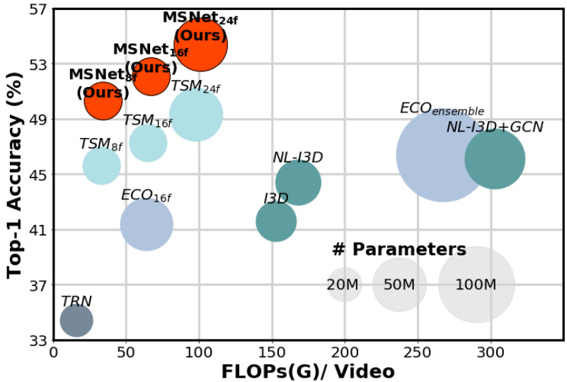
Fig. 1: Video classification performance comparison on Something-SomethingV1 [10] in terms of accuracy, computational cost, and model size. The proposed method (MSNet) achieves the best trade-off between accuracy and efficiency compared to state-of-the-art methods of TSM [21], TRN [47], ECO [48], I3D [2], NL-I3D [41], and GCN [42]. Best viewed in color.
图 1: Something-SomethingV1 [10] 数据集上视频分类性能对比 (准确率、计算成本和模型大小)。所提方法 (MSNet) 在准确率与效率的平衡上优于当前最优方法 TSM [21]、TRN [47]、ECO [48]、I3D [2]、NL-I3D [41] 和 GCN [42]。建议彩色查看。
To tackle the limitation of the existing methods, we propose an end-to-end trainable block, dubbed the Motion Squeeze (MS) module, for effective motion estimation. Inserted in the middle of any neural network for video understanding, it learns to establish correspondences across adjacent frames efficiently and convert them into effective motion features. The resultant motion features are readily fed to the next downstream layer and used for final prediction. To validate the proposed MS module, we develop a video classification architecture, dubbed the Motion Squeeze network (MSNet), that is equipped with the MS module. In comparison with recent methods, shown in Figure 1, the proposed method provides the best trade-off in terms of accuracy, computational cost, and model size in video understanding.
为解决现有方法的局限性,我们提出了一种名为运动压缩 (Motion Squeeze, MS) 模块的端到端可训练单元,用于高效运动估计。该模块可嵌入任何视频理解神经网络的中间层,通过学习高效建立相邻帧间的对应关系,并将其转化为有效的运动特征。生成的运动特征可直接输入下游网络层,用于最终预测。为验证所提出的MS模块,我们开发了配备该模块的视频分类架构——运动压缩网络 (Motion Squeeze Network, MSNet)。如图1所示,与现有方法相比,该方法在视频理解的准确率、计算成本和模型大小之间实现了最佳平衡。
2 Related work
2 相关工作
Video classification architectures. One of the main problems in video under standing is to categorize videos given a set of pre-defined target classes. Early methods based on deep neural networks have focused on learning spatio-temporal or motion features. Tran et al. [35] propose a 3D CNN (C3D) to learn spatiotemporal features while Simonyan and Zisserman [31] employ an independent temporal stream to learn motion features from pre computed optical flows. Carreira and Zisserman [2] design two-stream 3D CNNs (two-stream I3D) by integrating two former methods, and achieve the state-of-the-art performance at that time. As the two-stream 3D CNNs are powerful but computationally demanding, subsequent work has attempted to improve the efficiency. Tran et al. [37] and Xie et al. [43] propose to decompose 3D convolutional filters into 2D spatial and 1D temporal filters. Chen et al. [3] adopt group convolution techniques while Zolfaghari et al. [48] propose to study mixed 2D and 3D networks with the frame sampling method of temporal segment networks (TSN) [40]. Tran et al. [36] analyze the effect of 3D group convolutional networks and propose the channel-separated convolutional network (CSN). Lin et al. [21] propose the temporal shift module (TSM) that simulates 3D convolution using 2D convolution with a part of input feature channels shifted along the temporal axis. It enables 2D convolution networks to achieve a comparable classification accuracy to 3D CNNs. Unlike these approaches, we focus on efficient learning of motion features.
视频分类架构。视频理解中的一个主要问题是对给定一组预定义目标类别的视频进行分类。早期基于深度神经网络的方法主要集中于学习时空或运动特征。Tran等人[35]提出了一种3D CNN (C3D)来学习时空特征,而Simonyan和Zisserman[31]则采用独立的时间流从预计算的光流中学习运动特征。Carreira和Zisserman[2]通过整合前两种方法设计了两流3D CNN (two-stream I3D),并在当时取得了最先进的性能。由于两流3D CNN虽然强大但计算需求高,后续工作尝试提高效率。Tran等人[37]和Xie等人[43]提出将3D卷积滤波器分解为2D空间和1D时间滤波器。Chen等人[3]采用分组卷积技术,而Zolfaghari等人[48]提出研究混合2D和3D网络,并结合时间分段网络(TSN)[40]的帧采样方法。Tran等人[36]分析了3D分组卷积网络的效果,并提出了通道分离卷积网络(CSN)。Lin等人[21]提出了时间移位模块(TSM),通过沿时间轴移动部分输入特征通道来使用2D卷积模拟3D卷积。这使得2D卷积网络能够达到与3D CNN相当的分类精度。与这些方法不同,我们专注于运动特征的高效学习。
Learning motions in a video. While two-stream-based architectures [8,9,30, 31] have demonstrated the effectiveness of pre-computed optical flows, the use of optical flows typically degrades the efficiency of video processing. To address the issue, Ng et al. [26] use a multi-task learning of both optical flow estimation and action classification and Stroud et al. [32] propose to distill motion features from pre-trained two-stream 3D CNNs. These methods do not use pre-computed optical flows during inference, but still need them at the training phase. Other methods design network architectures that learn motions internally without external optical flows [7,16,20,27,34]. Sun et al. [34] compute spatial and temporal gradients between appearance features to learn motion features. Lee et al. [20] and Jiang et al. [16] propose a convolutional module to extract motion features by spatial shift and subtraction operation between appearance features. Despite their computational efficiency, they do not reach the classification accuracy of two-stream networks [31]. Fan et al. [7] implement the optimization process of TV-L1 [44] as iterative neural layers, and design an end-to-end trainable architecture (TVNet). Pier giovanni and Ryoo [27] extend the idea of TVNet by calculating channel-wise flows of feature maps at the intermediate layers of the CNN. These variation al methods achieve a good performance, but require a high computational cost due to iterative neural layers. In contrast, our method learns to extract effective motion features with a marginal increase of computation.
学习视频中的运动。虽然基于双流架构 [8,9,30,31] 已证明预计算光流的有效性,但使用光流通常会降低视频处理效率。为解决这一问题,Ng等人 [26] 采用光流估计与动作分类的多任务学习,Stroud等人 [32] 提出从预训练的双流3D CNN中蒸馏运动特征。这些方法在推理阶段无需预计算光流,但训练阶段仍需依赖光流。其他方法设计了无需外部光流即可内部学习运动的网络架构 [7,16,20,27,34]。Sun等人 [34] 通过计算外观特征间的空间和时间梯度来学习运动特征。Lee等人 [20] 和Jiang等人 [16] 提出卷积模块,通过外观特征的空间位移和减法操作提取运动特征。尽管计算高效,这些方法仍未达到双流网络 [31] 的分类精度。Fan等人 [7] 将TV-L1 [44] 优化过程实现为迭代神经层,设计了端到端可训练架构(TVNet)。Pier giovanni与Ryoo [27] 扩展TVNet思想,在CNN中间层计算特征图的通道级光流。这些变体方法性能优异,但因迭代神经层导致计算成本较高。相比之下,我们的方法能以边际计算量增长学习提取有效运动特征。
Learning visual correspondences. Our work is inspired by recent methods that learn visual correspondences between images using neural networks [6, 11, 19,24,28,33]. Fischer et al. [6] estimate optical flows using a convolutional neural network, which construct a correlation tensor from feature maps and regresses displacements from it. Sun et al. [33] use a stack of correlation layers for coarseto-fine optical flow estimation. While these methods require dense ground-truth optical flows in training, the structure of correlation computation and subsequent displacement estimation is widely adopted in other correspondence problems with different levels of supervision. For example, recent methods for semantic correspondence, i.e., matching images with intra-class variation, typically follow a similar pipeline to learn geometric transformation between images in a more weakly-supervised regime [11, 19, 24, 28]. In this work, motivated by this line of research, we develop a motion feature module that does not require any correspondence supervision for learning.
学习视觉对应关系。我们的工作受到近期使用神经网络学习图像间视觉对应关系的方法的启发 [6, 11, 19, 24, 28, 33]。Fischer 等人 [6] 通过卷积神经网络估计光流,该方法从特征图构建相关性张量并回归位移。Sun 等人 [33] 使用堆叠的相关层进行由粗到细的光流估计。虽然这些方法在训练时需要密集的真实光流标注,但其相关性计算结构和后续位移估计框架已被广泛用于不同监督程度的其他对应问题。例如,近期处理语义对应(即匹配类内差异图像)的方法通常遵循类似流程,在更弱监督条件下学习图像间的几何变换 [11, 19, 24, 28]。受此研究路线启发,我们开发了一个无需任何对应监督即可学习的运动特征模块。
Similarly to our work, a few recent methods [22, 45] have attempted to incorporate correspondence information for video understanding. Zhao et al. [45] use correlation information between feature maps of consecutive frames to replace optical flows. The size of their full model, however, is comparable to the two-stream networks [31]. Liu et al. [22] propose the correspondences proposal (CP) module to learn correspondences in a video. Unlike ours, they focus on analyzing spatio-temporal relationship within the whole video, rather than motion, and the model is not fully differentiable and thus less effective in learning. In contrast, we introduce a fully-differentiable motion feature module that can be inserted in the middle of any neural network for video understanding.
与我们工作类似,近期的一些方法 [22, 45] 尝试整合对应关系信息以进行视频理解。Zhao等人 [45] 利用连续帧特征图间的相关性信息替代光流,但其完整模型尺寸与双流网络 [31] 相当。Liu等人 [22] 提出对应关系提议 (CP) 模块来学习视频中的对应关系。与我们的方法不同,他们侧重于分析整个视频的时空关系而非运动,且模型并非完全可微分,因此学习效果较差。相比之下,我们引入了完全可微分的运动特征模块,可插入任何视频理解神经网络的中间层。
The main contribution of this work is three-fold.
本工作的主要贡献有三方面。
3 Proposed approach
3 研究方法
The overall architecture for video understanding is illustrated in Figure 2. Let us assume a neural network that takes a video of $T$ frames as input and predicts the category of the video as output, where convolutional layers are used to transform input frames into frame-wise appearance features. The proposed motion feature module, dubbed Motion Squeeze (MS) module, is inserted to produce frame-wise motion features using pairs of adjacent appearance features. The resultant motion features are added to the appearance features for final prediction. In this section, we first explain the MS module, and describe the details of our network architecture for video understanding.
视频理解的整体架构如图 2 所示。假设有一个神经网络以 $T$ 帧视频作为输入并预测视频类别作为输出,其中卷积层用于将输入帧转换为逐帧的外观特征。我们提出的运动特征模块 (Motion Squeeze, MS) 被插入其中,利用相邻外观特征对生成逐帧运动特征。最终将运动特征与外观特征相加以进行最终预测。本节首先阐述 MS 模块的工作原理,随后详细介绍视频理解网络架构的具体实现。
3.1 Motion Squeeze (MS) module
3.1 运动压缩 (Motion Squeeze, MS) 模块
The MS module is a learnable motion feature extractor, which can replace the use of explicit optical flows for video understanding. As described in Figure 3, given two feature maps from adjacent frames, it learns to extract effective motion features in three steps: correlation computation, displacement estimation, and feature transformation.
MS模块是一个可学习的运动特征提取器,能够替代显式光流在视频理解中的应用。如图3所示,给定相邻帧的两个特征图,它通过三个步骤学习提取有效运动特征:相关性计算、位移估计和特征变换。
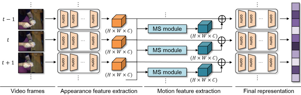
Fig. 2: Overall architecture of the proposed approach. The model first takes $T$ video frames as input and converts them into frame-wise appearance features using convolutional layers. The proposed Motion Squeeze (MS) module generates motion features using the frame-wise appearance features, and combines the motion features into the next downstream layer. $\bigoplus$ denotes element-wise addition.
图 2: 所提方法的整体架构。模型首先以 $T$ 帧视频作为输入,通过卷积层将其转换为逐帧外观特征。提出的运动压缩 (Motion Squeeze, MS) 模块利用逐帧外观特征生成运动特征,并将运动特征融合至下游网络层。$\bigoplus$ 表示逐元素相加。
Correlation computation. Let us denote the two adjacent input feature maps by $\mathbf{F}^{(t)}$ and $\mathbf{\deltaF}^{(t+1)}$ , each of which is 3D tensors of size $H\times W\times C$ . The spatial resolution is $H\times W$ and the $C$ dimensional features on spatial position $\mathbf{x}$ by $\mathbf{F_{x}}$ . A correlation score of position $\mathbf{x}$ with respect to displacement $\mathbf{p}$ is defined as
相关性计算。设相邻的两个输入特征图为 $\mathbf{F}^{(t)}$ 和 $\mathbf{\deltaF}^{(t+1)}$ ,它们都是尺寸为 $H\times W\times C$ 的3D张量。空间分辨率为 $H\times W$ ,空间位置 $\mathbf{x}$ 上的 $C$ 维特征记为 $\mathbf{F_{x}}$ 。位置 $\mathbf{x}$ 相对于位移 $\mathbf{p}$ 的相关性得分定义为
$$
s(\mathbf{x},\mathbf{p},t)=\mathbf{F}{\mathbf{x}}^{(t)}\cdot\mathbf{F}_{\mathbf{x}+\mathbf{p}}^{(t+1)},
$$
$$
s(\mathbf{x},\mathbf{p},t)=\mathbf{F}{\mathbf{x}}^{(t)}\cdot\mathbf{F}_{\mathbf{x}+\mathbf{p}}^{(t+1)},
$$
where denotes dot product. For efficiency, we compute the correlation scores of position $\mathbf{x}$ only in its neighborhood of size $P=2k+1$ by restricting a maximum displacement: $\mathbf{p}\in[-k,k]^{2}$ . For $t_{\mathrm{th}}$ frame, a resultant correlation tensor $\mathbf{S}^{(t)}$ is of size $H\times W\times P^{2}$ . The cost of computing the correlation tensor is equivalent to that of $1\times1$ convolutions with $P^{2}$ kernels; the correlation computation can be implemented as 2D convolutions on $t_{\mathrm{th}}$ feature map using $t+1_{\mathrm{th}}$ feature map as $P^{2}$ kernels. The total FLOPs in a single video amounts to $T H W C P^{2}$ . We apply a convolution layer before computing correlations, which learns to weight informative feature channels for learning visual correspondences. In practice, we set the neighborhood $P=15$ given the spatial resolution $28\times28$ and apply an $1\times1\times1$ layer with $C/2$ channels. For correlation computation, we adopt C++/Cuda implemented version of correlation layer in FlowNet [6].
其中·表示点积。为提高效率,我们仅计算位置$\mathbf{x}$在其大小为$P=2k+1$邻域内的相关性分数,通过限制最大位移量:$\mathbf{p}\in[-k,k]^{2}$。对于第$t_{\mathrm{th}}$帧,生成的关联张量$\mathbf{S}^{(t)}$尺寸为$H\times W\times P^{2}$。计算关联张量的开销相当于使用$P^{2}$个核进行$1\times1$卷积运算;该相关性计算可通过对第$t_{\mathrm{th}}$特征图实施2D卷积实现,其中将第$t+1_{\mathrm{th}}$特征图作为$P^{2}$个卷积核。单段视频的总FLOPs运算量为$T H W C P^{2}$。我们在计算相关性前应用卷积层,该层通过加权信息特征通道来学习视觉对应关系。实践中,在空间分辨率为$28\times28$时设置邻域$P=15$,并应用通道数为$C/2$的$1\times1\times1$卷积层。相关性计算采用FlowNet [6]中C++/Cuda实现的关联层版本。
Displacement estimation. From the correlation tensor $\mathbf{S}^{(t)}$ , we estimate a displacement field for motion information. A straightforward but non-differentiable method would be to take the best matching displacement for position x by argmaxp $s(\mathbf{x},\mathbf{p},t)$ . To make the operation differentiable, we can use a weighted average of displacements using softmax, called soft-argmax [13, 19], which is de
位移估计。从相关张量 $\mathbf{S}^{(t)}$ 中,我们估计一个位移场以获取运动信息。一个直接但不可微的方法是使用 argmaxp $s(\mathbf{x},\mathbf{p},t)$ 来获取位置 x 的最佳匹配位移。为了使该操作可微,我们可以使用 softmax 加权的位移平均值,称为 soft-argmax [13, 19]。
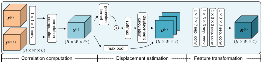
Fig. 3: Overall process of Motion Squeeze (MS) module. The MS module estimates motion across two frame-wise feature maps $(\mathbf{F}^{(t)},\mathbf{F}^{(t+1)})$ of adjacent frames. A correlation tensor $\mathbf{S}^{(t)}$ is obtained by computing correlations, and then a displacement tensor $\mathbf{D}^{(t)}$ is estimated using the tensor. Through the transformation process of convolution layers, the final motion feature $\mathbf{M}^{(t)}$ is obtained. See text for details.
图 3: Motion Squeeze (MS) 模块的整体流程。MS模块通过相邻帧的两个逐帧特征图 $(\mathbf{F}^{(t)},\mathbf{F}^{(t+1)})$ 估计运动。通过计算相关性获得相关张量 $\mathbf{S}^{(t)}$,随后利用该张量估计位移张量 $\mathbf{D}^{(t)}$。经过卷积层的变换处理,最终得到运动特征 $\mathbf{M}^{(t)}$。详见正文说明。
fined as
定义为
$$
d(\mathbf{x},t)=\sum_{\mathbf{p}}{\frac{\exp(s(\mathbf{x},\mathbf{p},t))}{\sum_{\mathbf{p^{\prime}}}\exp(s(\mathbf{x},\mathbf{p^{\prime}},t))}}\mathbf{p}.
$$
$$
d(\mathbf{x},t)=\sum_{\mathbf{p}}{\frac{\exp(s(\mathbf{x},\mathbf{p},t))}{\sum_{\mathbf{p^{\prime}}}\exp(s(\mathbf{x},\mathbf{p^{\prime}},t))}}\mathbf{p}.
$$
This method, however, is sensitive to noisy outliers in the correlation tensor since it is influenced by all correlation values. We thus use the kernel-soft-argmax [19] that suppresses such outliers by masking a 2D Gaussian kernel on the correlation values; the kernel is centered on each target position so that the estimation is more influenced by closer neighbors. Our kernel-soft-argmax for displacement estimation is defined as
然而,该方法对相关张量中的噪声异常值敏感,因为它会受到所有相关值的影响。因此,我们使用核软最大值 (kernel-soft-argmax) [19],通过在相关值上掩码一个二维高斯核来抑制此类异常值;该核以每个目标位置为中心,使得估计更受邻近值的影响。我们用于位移估计的核软最大值定义为
$$
d(\mathbf{x},t)=\sum_{\mathbf{p}}\frac{\exp(g(\mathbf{x},\mathbf{p},t)s(\mathbf{x},\mathbf{p},t)/\tau)}{\sum_{\mathbf{p^{\prime}}}\exp(g(\mathbf{x},\mathbf{p^{\prime}},t)s(\mathbf{x},\mathbf{p^{\prime}},t)/\tau)}\mathbf{p},
$$
$$
d(\mathbf{x},t)=\sum_{\mathbf{p}}\frac{\exp(g(\mathbf{x},\mathbf{p},t)s(\mathbf{x},\mathbf{p},t)/\tau)}{\sum_{\mathbf{p^{\prime}}}\exp(g(\mathbf{x},\mathbf{p^{\prime}},t)s(\mathbf{x},\mathbf{p^{\prime}},t)/\tau)}\mathbf{p},
$$
where
哪里
$$
g(\mathbf{x},\mathbf{p},t)=\frac{1}{\sqrt{2\pi}\sigma}\exp(\frac{\mathbf{p}-\mathrm{argmax}_{\mathbf{p}}s(\mathbf{x},\mathbf{p},t)}{\sigma^{2}}).
$$
$$
g(\mathbf{x},\mathbf{p},t)=\frac{1}{\sqrt{2\pi}\sigma}\exp(\frac{\mathbf{p}-\mathrm{argmax}_{\mathbf{p}}s(\mathbf{x},\mathbf{p},t)}{\sigma^{2}}).
$$
Note that $g(\mathbf{x},\mathbf{p},t)$ is the Gaussian kernel and we empirically set the standard deviation $\sigma$ to $5$ . $\tau$ is a temperature factor adjusting the softmax distribution; as $\tau$ decreases, softmax approaches argmax. We set $\tau=0.01$ in our experiments.
注意 $g(\mathbf{x},\mathbf{p},t)$ 是高斯核 (Gaussian kernel) ,我们经验性地将标准差 $\sigma$ 设为 $5$ 。 $\tau$ 是调节 softmax 分布的温度因子;随着 $\tau$ 减小,softmax 会趋近于 argmax。实验中我们设 $\tau=0.01$ 。
In addition to the estimated displacement map, we use a confidence map of correlation as auxiliary motion information, which is obtained by pooling the highest correlation on each position $\mathbf{x}$ :
除了估计的位移图外,我们还使用相关性置信图作为辅助运动信息,该图通过汇集每个位置 $\mathbf{x}$ 上的最高相关性获得:
$$
s^{}(\mathbf{x},t)=\operatorname*{max}_{\mathbf{p}}s(\mathbf{x},\mathbf{p},t).
$$
$$
s^{}(\mathbf{x},t)=\operatorname*{max}_{\mathbf{p}}s(\mathbf{x},\mathbf{p},t).
$$
The confidence map may be useful for identifying displacement outliers and learning informative motion features.
置信度图可能有助于识别位移异常值并学习有意义的运动特征。
We concatenate the (2-channel) displacement map and the (1-channel) confidence map into a displacement tensor $\mathbf{D}^{(t)}$ of size $H\times W\times3$ for the next step of motion feature transformation. An example of them is visualized in Figure 4.
我们将 (2通道) 位移图和 (1通道) 置信度图拼接成一个尺寸为 $H\times W\times3$ 的位移张量 $\mathbf{D}^{(t)}$ ,用于下一步的运动特征变换。图 4 展示了它们的可视化示例。
Feature transformation. We convert the displacement tensor $\mathbf{D}^{(t)}$ to an effective motion feature $\mathbf{M}^{(t)}$ that is readily incorporated into downstream layers. The tensor $\mathbf{D}^{(t)}$ is fed to four depth-wise separable convolution [14] layers, one $1\times7\times7$ layer followed by three $1\times3\times3$ layers, and transformed into a motion feature $\mathbf{M}^{(t)}$ with the same number of channels $C$ as that of the original input $\mathbf{F}^{(t)}$ . The depth-wise separable convolution approximates 2D convolution with a significantly less computational cost [4, 29, 36]. Note that all depth-wise and point-wise convolution layers are followed by batch normalization [15] and ReLU [25]. As in the temporal stream layers of [31], this feature transformation process is designed to learn task-specific motion features with convolution layers by interpreting the semantics of displacement and confidence. As illustrated in Figure 2, the MS module generates motion feature $\mathbf{M}^{(t)}$ using two adjacent appearance features $\mathbf{F}^{(t)}$ and $\mathbf{\deltaF}^{(t+1)}$ and then add it to the input of the next layer. Given $T$ frames, we simply pad the final motion feature $\mathbf{M}^{(T)}$ with $\mathbf{M}^{(T-1)}$ by setting $\mathbf{M}^{(T)}=\mathbf{M}^{(T-1)}$ .
特征转换。我们将位移张量 $\mathbf{D}^{(t)}$ 转换为易于融入下游层的有效运动特征 $\mathbf{M}^{(t)}$。该张量经过四个深度可分离卷积层 [14] 处理(一个 $1\times7\times7$ 层和三个 $1\times3\times3$ 层),转化为与原始输入 $\mathbf{F}^{(t)}$ 通道数 $C$ 相同的运动特征 $\mathbf{M}^{(t)}$。深度可分离卷积能以显著更低计算成本 [4, 29, 36] 近似二维卷积。所有深度卷积和逐点卷积层后都接批量归一化 [15] 和 ReLU 激活 [25]。如文献 [31] 时序流层设计,该转换过程通过卷积层解析位移与置信度的语义信息来学习任务相关运动特征。如图 2 所示,MS 模块利用相邻外观特征 $\mathbf{F}^{(t)}$ 与 $\mathbf{\deltaF}^{(t+1)}$ 生成运动特征 $\mathbf{M}^{(t)}$,并将其叠加至下一层输入。对于 $T$ 帧序列,我们通过设定 $\mathbf{M}^{(T)}=\mathbf{M}^{(T-1)}$ 用 $\mathbf{M}^{(T-1)}$ 对末帧运动特征进行填充。
3.2 Motion Squeeze network (MSNet).
3.2 运动压缩网络 (MSNet)
The MS module can be inserted into any video understanding architecture to improve the performance by motion feature modeling. In this work, we introduce standard convolutional neural networks (CNNs) with the MS module, dubbed MSNet, for video classification. We adopt the ImageNet-pretrained ResNet [12] as the CNN backbone and insert TSM [21] for each residual block of the ResNet. TSM enables 2D convolution to obtain the effect of 3D convolution by shifting a part of input feature channels along the temporal axis before the convolution operation. Following the default setting in [21], we shift 1/8 of the input features channels forward and another $1/8$ of the channels backward in each TSM.
MS模块可通过运动特征建模提升性能,可嵌入任何视频理解架构。本研究将标准卷积神经网络(CNN)与MS模块结合,提出MSNet视频分类框架。我们采用ImageNet预训练的ResNet[12]作为CNN主干网络,并在每个残差块中插入TSM[21]。TSM通过沿时间轴偏移部分输入特征通道再进行卷积运算,使2D卷积获得3D卷积的效果。遵循[21]的默认设置,每个TSM模块中我们向前偏移1/8输入特征通道,向后偏移$1/8$通道。
The overall architecture of the proposed model is shown in Figure 2; a single MS module is inserted after the third stage of the ResNet. We fuse the motion feature into the appearance feature by element-wise addition:
所提模型的整体架构如图 2 所示;在 ResNet 的第三阶段后插入了一个单独的 MS (Motion Stream) 模块。我们通过逐元素相加的方式将运动特征融合到外观特征中:
$$
\mathbf{F}^{\prime(t)}=\mathbf{F}^{(t)}+\mathbf{M}^{(t)}.
$$
$$
\mathbf{F}^{\prime(t)}=\mathbf{F}^{(t)}+\mathbf{M}^{(t)}.
$$
In section 4.5, we extensively evaluate different fusion methods, e.g., concatenation and multiplication, and show that additive fusion is better than the others. After fusing both features, the combined feature is passed through the next downstream layers. The network outputs over $T$ frames are temporally averaged to produce a final output and the cross-entropy with softmax is used as a loss function for training. By default setting, MSNet learns both appearance and motion features jointly in a single network at the cost of only 2.5% and $1.2%$ increase in FLOPs and the number of parameters, respectively.
在4.5节中,我们全面评估了不同的融合方法(如拼接和乘法),并证明加法融合优于其他方法。融合两种特征后,组合特征会传递至下游网络层。网络在$T$帧上的输出经过时序平均生成最终结果,并采用带softmax的交叉熵作为训练损失函数。默认配置下,MSNet以仅增加2.5% FLOPs和$1.2%$参数量为代价,在单一网络中联合学习外观与运动特征。
4 Experiments
4 实验
4.1 Datasets
4.1 数据集
Something-Something V1&V2 [10] are trimmed video datasets for human action classification. Both datasets consist of 174 classes with 108,499 and 220,847 videos in total, respectively. Each video contains one action and the duration spans from 2 to 6 seconds. Something-Something V1&V2 are motion-oriented datasets where temporal relationships are more salient than in others.
Something-Something V1&V2 [10] 是用于人类动作分类的剪辑视频数据集。两个数据集分别包含174个类别,总计108,499和220,847个视频。每个视频包含一个动作,时长介于2至6秒之间。Something-Something V1&V2是以动作为导向的数据集,其时间关系比其他数据集更为显著。
Kinetics [17] is a popular large-scale video dataset, consisting of 400 classes with over 250,000 videos. Each video lasts around 10 seconds with a single action. HMDB51 [18] contains 51 classes with 6,766 videos. Kinetics and HMDB-51 focus more on appearance information rather than motion.
Kinetics [17] 是一个流行的大规模视频数据集,包含400个类别超过25万段视频。每段视频时长约10秒,记录单个动作。HMDB51 [18] 包含51个类别共6,766段视频。Kinetics和HMDB-51更侧重于外观信息而非运动信息。
4.2 Implementation details
4.2 实现细节
Clip sampling. In both training and testing, instead of an entire video, we use a clip of frames that are sampled from the video. We use the segment-based sampling method [40] for the Something-Something V1&V2 while adopting the dense frame sampling method [2] for Kinetics and HMDB-51.
片段采样。在训练和测试过程中,我们不是使用整个视频,而是从视频中采样一个帧片段。对于Something-Something V1&V2数据集采用基于片段的采样方法[40],而对Kinetics和HMDB-51数据集则采用密集帧采样方法[2]。
Training. For each video, we sample a clip of 8 or 16 frames, resize them into $240\times320$ images, and crop $224\times224$ images from the resized images [48]. The minibatch SGD with Nestrov momentum is used for optimization, and the batch size is set to 48. We use scale jittering for data augmentation. For the SomethingSomething V1&V2, we set the training epochs to 40 and the initial learning rate to 0.01; the learning rate is decayed by $1/10$ after $20_{\mathrm{th}}$ and $30_{\mathrm{th}}$ epochs. For Kinetics, we set the training epochs to 80 and the initial learning rate to 0.01; the learning rate is decayed by $1/10$ after 40 and 60 epochs. In training our model on HMDB-51, we fine-tune the Kinetics-pretrained model as in [21, 37]. We set the training epochs to 35 and the initial learning rate to 0.001; the learning rate is decayed by 1/10 after $15_{\mathrm{th}}$ and $30_{\mathrm{th}}$ epochs.
训练。对于每个视频,我们采样包含8或16帧的片段,将其缩放为$240\times320$的图像,并从缩放后的图像中裁剪出$224\times224$的图像[48]。优化采用带Nestrov动量的minibatch SGD(随机梯度下降),批量大小设为48。数据增强采用尺度抖动策略。在SomethingSomething V1&V2数据集上,训练周期设为40轮,初始学习率为0.01;学习率在第20轮和第30轮后衰减为$1/10$。Kinetics数据集上设置80轮训练周期,初始学习率0.01;学习率在第40轮和第60轮后衰减$1/10$。在HMDB-51数据集上微调Kinetics预训练模型时[21,37],训练周期设为35轮,初始学习率0.001;学习率在第15轮和第30轮后衰减1/10。
Inference. Given a video, we sample a clip and test its center crop. For SomethingSomething V1&V2, we evaluate both the single clip prediction and the average prediction of 10 randomly-sampled clips. For Kinetics and HMDB-51, we evaluate the average prediction of uniformly-sampled 10 clips from each video.
推理。给定一段视频,我们采样一个片段并测试其中间区域。对于SomethingSomething V1&V2,我们评估单片段预测结果和10个随机采样片段的平均预测结果。对于Kinetics和HMDB-51,我们评估从每段视频中均匀采样10个片段的平均预测结果。
4.3 Comparison with state-of-the-art methods
4.3 与最先进方法的对比
Table 1 summarizes the results on Something-Something V1&V2. Each section of the table contains results of 2D CNN methods [20, 22, 40, 47], 3D CNN methods [16, 23, 42, 43, 48], ResNet with TSM (TSM ResNet) [21], and the proposed method, respectively. Most of the results are copied from the corresponding papers, except for TSM ResNet; we evaluate the official pre-trained model of TSM ResNet using a single center-cropped clip per video in terms of top-1 and top-5 accuracies. Our method, which uses TSM ResNet as a backbone, achieves $50.9%$ and $63.0%$ on Something-Something V1 and V2 at top-1 accuracy, respectively, which outperforms most of 2D CNN and 3D CNN methods, while using a single clip with 8 input frames only. Compared to the TSM ResNet baseline, our method obtains a significant gain of about 5.3% points and 4.2% points at top-1 accuracy at the cost of only $2.5%$ and $1.2%$ increase in FLOPs and parameters, respectively. When using 16 frames, our method further improves achieving $52.1%$ and $64.7%$ at top-1 accuracy, respectively. Following the evaluation procedure of two-stream networks, we evaluate the ensemble model (MSNet-R50 $_{E n}$ ) by averaging prediction scores of the 8-frame and 16-frame models. With the same number of clips for evaluation, it achieves top-1 accuracy 1.8% points and $1.6%$ points higher than TSM two-stream networks with 22% less computation, even no optical flow needed. Our 10-clip model achieves $55.1%$ and $67.1%$ at top-1 accuracy on Something-Something V1 and V2, respectively, which is the state-of-the-art on both of the datasets. As shown in Figure 1, our model provides the best trade-off in terms of accuracy, FLOPs, and the number of parameters.
表 1: 总结了Something-Something V1&V2上的结果。表格的每个部分分别包含2D CNN方法[20, 22, 40, 47]、3D CNN方法[16, 23, 42, 43, 48]、带TSM的ResNet (TSM ResNet)[21]以及所提方法的结果。除TSM ResNet外,大多数结果都是从相应论文中复制的;我们使用每个视频单中心裁剪片段评估了TSM ResNet官方预训练模型的top-1和top-5准确率。以TSM ResNet为骨干网络的方法在Something-Something V1和V2上分别达到50.9%和63.0%的top-1准确率,优于大多数2D CNN和3D CNN方法,且仅使用8输入帧的单片段。相比TSM ResNet基线,该方法在top-1准确率上分别获得约5.3%和4.2%的显著提升,而FLOPs和参数量仅分别增加2.5%和1.2%。当使用16帧时,该方法进一步提升至52.1%和64.7%的top-1准确率。遵循双流网络评估流程,我们通过对8帧和16帧模型的预测分数取平均来评估集成模型(MSNet-R50$_{En}$)。在相同评估片段数下,其top-1准确率比TSM双流网络高1.8%和1.6%,且计算量减少22%,无需光流。10片段模型在Something-Something V1和V2上分别达到55.1%和67.1%的top-1准确率,在两个数据集上均达到最先进水平。如图1所示,我们的模型在准确率、FLOPs和参数量之间实现了最佳平衡。
Table 1: Performance comparison on Something-Something V1&V2. The symbol $\dagger$ denotes the reproduced by ours.
表 1: Something-Something V1&V2 性能对比。符号 $\dagger$ 表示我们复现的结果。
| model | fow #frame | FLOPs Xclips | #param | SomethingV1 top-1 | top-5 | SomethingV2 top-5 |
|---|---|---|---|---|---|---|
| TSN [40] | 8 | 16Gx1 | 10.7M | 19.5 | 33.4 | |
| TRN [47] | 8 | 16GxN/A | 18.3M | 34.4 | - | 48.8 |
| TRN Two-stream [47] | 8+8 | 16GxN/A | 18.3M | 42.0 | 55.5 | |
| MFNet [20] | 10 | N/Ax10 | 43.9 | 73.1 | ||
| CPNet [22] | 24 | N/Ax96 | - | 57.7 | ||
| ECOEnLite [48] | 92 | 267x1 | 150M | 46.4 | - | |
| ECO Two-stream [48] | 92+92 | N/Ax1 | 300M | 49.5 | ||
| I3D from [42] | 32 | 153Gx2 | 28.0M | 41.6 | 72.2 | |
| NL-I3D from [42] | 32 | 168Gx2 | 35.3M | 44.4 | 76.0 | |
| NL-I3D+GCN [42] | 32 | 303Gx2 | 62.2M | 46.1 | 76.8 | |
| S3D-G [43] | 64 | 71Gx1 | 11.6M | 48.2 | 78.7 | |
| DFB-Net [23] | 16 | N/Ax1 | 50.1 | 79.5 | ||
| STM [16] | 16 | 67G×30 | 24.0M | 50.7 | 80.4 | 64.2 |
| TSM [21] | 8 | 33Gx1 | 24.3M | 45.6 | 74.2 | 58.8 |
| TSM 21 | 16 | 65Gx1 | 24.3M | 47.3 | 77.1 | 61.2 |
| TSMEn [21] | 16+8 | 98G×1 | 48.6M | 49.7 | 78.5 | 62.9 |
| TSM Two-stream | 16+16 | 129Gx1 | 48.6M | 52.6 | 81.9 | 65.0t |
| TSM Two-stream 21 | 16+16 | 129Gx6 | 48.6M | 66.0 | ||
| MSNet-R50 (ours) | 8 | 34Gx1 | 24.6M | 50.9 | 80.3 | 63.0 |
| MSNet-R50 (ours) | 16 | 67Gx1 | 24.6M | 52.1 | 82.3 | 64.7 |
| MSNet-R50En (ours) | 16+8 | 101Gx1 | 49.2M | 54.4 | 83.8 | 66.6 |
| MSNet-R50En (ours) | 16+8 | 101Gx10 | 49.2M | 55.1 | 84.0 | 67.1 |
4.4 Comparison with other motion representation methods
4.4 与其他运动表示方法的对比
Table 2 summarizes comparative results with other motion representation methods [7, 16, 20, 27, 34] based on RGB frames. The comparison is done on Kinetics and HMDB51 since the previous methods commonly report their results on them. Each section of the table contains results of conventional 2D and 3D
表 2: 总结了基于RGB帧的其他运动表示方法 [7, 16, 20, 27, 34] 的对比结果。由于先前方法通常在Kinetics和HMDB51上报告结果,因此比较在这两个数据集上进行。表格的每个部分包含传统2D和3D方法的结果。
Table 2: Performance comparison with motion representation methods. The symbol $^\ddag$ denotes that we only report the backbone FLOPs.
表 2: 运动表示方法性能对比。符号 $^\ddag$ 表示我们仅报告主干 FLOPs。
| model | flow#frame | FLOPs xclips | (V/s) | speed Kinetics HMDB51 Top-1 | Top-1 |
|---|---|---|---|---|---|
| ResNet-50 from [27] | 32 | 132Gx25 | 22.8 | 61.3 | 59.4 |
| R(2+1)D [37] | 32 | 152Gx115 | 8.7 | 72.0 | 74.3 |
| MFNet from [27] | 10 | 80G+×10 | 56.8 | ||
| OFF(RGB)[34] | 1 | N/Ax25 | 57.1 | ||
| TVNet [7] | 18 | N/Ax250 | 71.0 | ||
| STM [16] | 16 | 67Gx30 | 73.7 | 72.2 | |
| Rep-flow (ResNet-50) [27] | 32 | 132G+×25 | 3.7 | 68.5 | 76.4 |
| Rep-fow (R(2+1)D) [27] | 32 | 152G+×25 | 2.0 | 75.5 | 77.1 |
| ResNet-50 Two-stream from [27] | 32+32 | 264Gx25 | 0.2 | 64.5 | 66.6 |
| R(2+1)D Two-stream [37] | 32+32 | 304Gx115 | 0.2 | 73.9 | 78.7 |
| OFF(RGB+Flow+RGB Diff)[34] | 1+5+5 | N/Ax25 | - | 74.2 | |
| TSM (reproduced) | 8 | 33G×10 | 64.1 | 73.5 | 71.9 |
| MSNet-R50(ours) | 8 | 34Gx10 | 54.2 | 75.0 | 75.8 |
| MSNet-R50 (ours) | 16 | 67Gx10 | 31.2 | 76.4 | 77.4 |
CNNs, motion representation methods [7, 16, 20, 27, 34], two-stream CNNs with optical flows [12, 37], and the proposed method, respectively. OFF, MFNet, and STM [16,20,34] use a sub-network or lightweight modules to calculate temporal gradients of frame-wise feature maps. TVNet [7] and Rep-flow [27] internalize iterative TV-L1 flow operations in their networks. As shown in Table 2, the proposed model using 16 frames outperforms all the other conventional CNNs and the motion representation methods [2, 7, 12, 16, 20, 27, 34, 37], while being competitive with the R(2+1)D two-stream [37] that uses pre-computed optical flows. Furthermore, our model is highly efficient than all the other methods in terms of FLOPs, clips, and the number of frames.
CNN、运动表征方法 [7, 16, 20, 27, 34]、带光流的两流CNN [12, 37] 以及本文提出的方法。OFF、MFNet和STM [16,20,34] 使用子网络或轻量级模块计算逐帧特征图的时间梯度。TVNet [7] 和Rep-flow [27] 在其网络中内化了迭代TV-L1光流运算。如表2所示,使用16帧的提出模型优于所有其他传统CNN和运动表征方法 [2, 7, 12, 16, 20, 27, 34, 37],同时与使用预计算光流的R(2+1)D双流方法 [37] 具有竞争力。此外,我们的模型在FLOPs、片段数和帧数方面均比其他方法更高效。
Run-time. We also evaluate in Table 2 the inference speeds of several models to demonstrate the efficiency of our method. All the run-times reported are measured on a single GTX Titan Xp GPU, ignoring the time of data loading. For this experiment, we set the spatial size of the input to $224\times224$ and the batch size to 1. The official codes are used for ResNet, TSM ResNet, and Repflow [12, 21, 27] except for R(2+1)D [37] we implemented. In evaluating Repflow [27], we use 20 iterations for optimization as in the original paper. The speed of the two-stream networks [31, 37] includes computation time for TV-L1 method on the GPU. The run-time results clearly show the cost of iterative optimization s used in two-stream networks and Rep-flow. In contrast, our model using 16 frames is about 160 $\times$ faster than the two-stream networks. Compared to Rep-flow ResNet-50, our method performs about 4 $\times$ faster due to the absence of the iterative optimization process in Rep-flow.
运行时。我们还在表2中评估了几种模型的推理速度,以展示本方法的高效性。所有运行时间均在单块GTX Titan Xp GPU上测量,不含数据加载耗时。本实验设定输入空间尺寸为$224\times224$,批次大小为1。除自行实现的R(2+1)D [37]外,ResNet、TSM ResNet和Repflow [12, 21, 27]均采用官方代码。评估Repflow [27]时,我们按照原论文使用20次优化迭代。双流网络 [31, 37]的速度包含GPU端TV-L1方法的计算耗时。运行时结果清晰表明双流网络与Rep-flow采用的迭代优化成本较高。相比之下,我们使用16帧的模型比双流网络快约160$\times$。相较于Rep-flow ResNet-50,由于省去了Rep-flow的迭代优化过程,我们的方法实现了约4$\times$的速度提升。
Table 3: Performance comparison with different displacement estimations.
表 3: 不同位移估计的性能对比
| model | FLOPs | top-1 | top-5 |
|---|---|---|---|
| baseline | 14.6G | 41.5 | 71.8 |
| S | 14.8G | 43.8 | 74.9 |
| KS | 14.9G | 44.6 | 75.4 |
| KS + CM | 14.9G | 45.5 | 76.5 |
| KS + CM + BD | 15.1G | 46.0 | 76.7 |

Fig. 4: Top-1 accuracy and FLOPs with different patch sizes.
图 4: 不同分块(patch)尺寸下的Top-1准确率与FLOPs对比
Table 4: Performance comparison with different positions of the MS module.
表 4: MS模块不同位置下的性能对比
| 模型 | FLOPs | top-1 | top-5 |
|---|---|---|---|
| baseline | 14.6G | 41.5 | 71.8 |
| res2 | 15.6G | 45.1 | 76.1 |
| res3 | 14.9G | 45.5 | 76.5 |
| res4 | 14.7G | 42.6 | 73.2 |
| res5 | 14.6G | 41.1 | 71.8 |
| res2,3,4 | 16.0G | 45.7 | 76.8 |
Table 5: Performance comparison with different fusing strategies.
表 5: 不同融合策略的性能对比。
| model | FLOPs | top-1 | top-5 |
|---|---|---|---|
| baseline | 14.6G | 41.5 | 71.8 |
| MS only | 14.1G | 38.8 | 70.7 |
| multiply | 14.9G | 44.5 | 75.9 |
| concat. | 15.7G | 45.0 | 76.1 |
| add | 14.9G | 45.5 | 76.5 |
4.5 Ablation studies
4.5 消融实验
We conduct ablation studies of the proposed method on Something-Something V1 [10] dataset. We use ImageNet pre-trained TSM ResNet-18 as a default backbone and use 8 input frames for all experiments in this section.
我们在Something-Something V1 [10]数据集上对提出的方法进行了消融研究。本节所有实验均采用ImageNet预训练的TSM ResNet-18作为默认主干网络,并使用8帧输入。
Displacement estimation in MS module. In Table 3, we experiment with different variants of the displacement tensor $\mathbf{D}^{(t)}$ in the MS module. We first compare soft-argmax (‘S’) and kernel-soft-argmax (‘KS’) for displacement estimation. As shown in the upper part of Table 3. the kernel-soft-argmax outperforms the soft-argmax, showing the noise reduction effect of Gaussian kernel. In the lower part of Table 3, we evaluate the effect of additional features: confidence maps (‘CM’) and backward displacement tensor (‘BD’). The backward displacement tensor is estimated from $\mathbf{\boldsymbol{F}}^{(t+1)}$ to $\mathbf{F}^{(t)}$ . We concatenate the forward and backward displacement tensors, and then pass them to the feature transformation layers. We obtain $0.9%$ points gain by appending the confidence map to the displacement tensor. Furthermore, by adding backward displacement we obtain another $0.5%$ points gain at top-1 accuracy, indicating that forward and backward displacement maps complement each other to enrich motion information. We use the kernel-soft-argmax with the confidence map $(^{\cdot}\mathrm{KS}+\mathrm{CM}^{,}$ ) as a default method for all other experiments.
MS模块中的位移估计。在表3中,我们实验了MS模块中位移张量$\mathbf{D}^{(t)}$的不同变体。首先比较了软最大值('S')和核软最大值('KS')在位移估计中的表现。如表3上半部分所示,核软最大值优于软最大值,展示了高斯核的降噪效果。在表3下半部分,我们评估了附加特征的影响:置信度图('CM')和后向位移张量('BD')。后向位移张量是从$\mathbf{\boldsymbol{F}}^{(t+1)}$到$\mathbf{F}^{(t)}$估计得到的。我们将前向和后向位移张量拼接后输入特征变换层。通过在位移张量上附加置信度图,我们获得了0.9%的性能提升。此外,通过添加后向位移,我们在top-1准确率上又获得了0.5%的提升,表明前向和后向位移图相互补充以丰富运动信息。我们将带置信度图的核软最大值$(^{\cdot}\mathrm{KS}+\mathrm{CM}^{,}$)作为所有其他实验的默认方法。
Size of matching region. In Figure 4, we evaluate performance varying the spatial size of matching regions of the MS module. Even with a small matching region $P=3$ , it provides a noticeable performance gain of over 2.7% points to the baseline. The performance tends to increase as the matching region becomes larger due to the larger displacement it can handle between frames. The performance is saturated after $P=15$ .
匹配区域大小。在图4中,我们评估了MS模块匹配区域空间尺寸变化对性能的影响。即使采用较小的匹配区域$P=3$,也能为基线带来超过2.7个百分点的显著性能提升。由于可处理帧间更大位移量,性能随着匹配区域扩大呈上升趋势。当$P=15$后性能趋于饱和。

Fig. 5: Top-1 accuracy and FLOPs with MS module on different backbones.
图 5: 不同骨干网络下 MS 模块的 Top-1 准确率与 FLOPs 对比。
Table 6: Performance comparison with twostream networks.
表 6: 双流网络性能对比
| model | flow | FLOPs | top-1 | top-5 |
|---|---|---|---|---|
| baseline | 14.6G | 41.5 | 71.8 | |
| Two-stream8+(8x5) | √ | 31.4G | 46.8 44.7 | 77.3 75.2 |
| Two-stream8+(8x1) Two-stream8+(8x1)(low) | √ | 28.9G 28.9G | 44.1 | 74.9 |
| MSNet | 14.9G | 45.5 | 76.5 |
Position of MS module. In Table 4, we evaluate different positions of the MS module. We denote that $r e s N$ by the $N$ -th stage of the ResNet. For each stage, it is inserted right after its final residual block. The result shows that while the MS module is beneficial in most cases, both accuracy and efficiency gains depend on the position of the module. It performs the best at $r e s_{3}$ ; appearance features from $r e s_{2}$ are not strong enough for accurate feature matching while spatial resolutions of appearance features from $r e s_{4}$ and $r e s_{5}$ are not high enough. The position of the module also affects FLOPs; the computational cost quadratically increases with spatial resolution due to convolution layers of the feature transformation. When inserting multiple MS modules $\left(r e s_{2,3,4}\right)$ at the backbone, it marginally improves top-1 accuracy as $0.2%$ points. Multiple modules appear to generate similar motion information even in different levels of features.
MS模块的位置。在表4中,我们评估了MS模块的不同位置。我们用$resN$表示ResNet的第$N$个阶段。每个阶段的MS模块都插入在其最后的残差块之后。结果表明,虽然MS模块在大多数情况下都有益,但准确性和效率的提升取决于模块的位置。在$res_{3}$处表现最佳;$res_{2}$的外观特征对于精确的特征匹配来说不够强,而$res_{4}$和$res_{5}$的外观特征空间分辨率不够高。模块的位置也会影响FLOPs;由于特征变换的卷积层,计算成本随着空间分辨率的增加呈二次方增长。当在骨干网络中插入多个MS模块$\left(res_{2,3,4}\right)$时,top-1准确率仅略微提高了$0.2%$。多个模块似乎在不同层次的特征中生成相似的运动信息。
Fusing strategy of MS module. In Table 5, we evaluate different fusion strategies for the MS module; ‘MS only’, ‘multiply’, ‘concat’, and ‘add’. In the case of ‘MS only’, we only pass $\mathbf{M}^{(t)}$ into downstream layers without $\mathbf{F}^{(t)}$ . We apply element-wise multiplication and element-wise addition, respectively, for ‘multiply’ and ‘add’. In the case of ‘concat’, we concatenate $\mathbf{F}^{(t)}$ and $\mathbf{M}^{(t)}$ , whose channel size is transformed to $C$ via an $1\times1\times1$ convolution layer. ‘MS only’ is less accurate than the baseline because visual semantic information is discarded. While both ‘multiply’ and ‘concat’ clearly improve the accuracy, ‘add’ achieves the best performance with $45.5%$ at top-1 accuracy. We find that additive fusion is the most effective and stable in amplifying appearance features of moving objects.
MS模块的融合策略。在表5中,我们评估了MS模块的不同融合策略:"仅MS"、"相乘"、"拼接"和"相加"。在"仅MS"情况下,我们仅将$\mathbf{M}^{(t)}$传递至下游层而不使用$\mathbf{F}^{(t)}$。对于"相乘"和"相加"策略,我们分别采用逐元素乘法和逐元素加法。在"拼接"情况下,我们将$\mathbf{F}^{(t)}$和$\mathbf{M}^{(t)}$通过$1\times1\times1$卷积层将通道数转换为$C$后进行拼接。"仅MS"策略由于丢弃了视觉语义信息,其准确率低于基线。虽然"相乘"和"拼接"策略都显著提升了准确率,但"相加"策略以45.5%的top-1准确率取得了最佳性能。我们发现加法融合在增强运动目标外观特征方面最为有效且稳定。
Effect of MS module on different backbones. In Figure 5, we also evaluate the effect of the MS module on ResNet-18, MobileNet-V2, and I3D. We insert one MS module where the spatial resolution of the feature map remains the same. For ResNet-18 and MobileNet-V2, we finetune models pre-trained on ImageNet.
MS模块对不同主干网络的影响。在图5中,我们还评估了MS模块在ResNet-18、MobileNet-V2和I3D上的效果。我们在特征图空间分辨率保持不变的位置插入一个MS模块。对于ResNet-18和MobileNet-V2,我们微调了在ImageNet上预训练的模型。
We train I3D from scratch. Our MS module benefits both 2D CNNs and 3D CNNs to obtain higher accuracy. The module significantly improves ResNet-18 and MobileNet-V2 by 21.3% and $19.2%$ points, respectively, in top-1 accuracy. Since 2D CNNs do not use any spatio-temporal features, it obtains significantly higher gain from the MS module. The MS module also improves I3D and TSM ResNet-18 by $2.4%$ and $4.0%$ points, respectively, in top-1 accuracy. The gain on 3D CNNs, although relatively small, verifies that the motion features by the MS module are complementary even to the spatio-temporal features; the MS module learns explicit motion information across adjacent frames whereas TSM covers long-term temporal length using (pseudo-)temporal convolutions.
我们从头开始训练I3D。我们的MS模块同时提升了2D CNN和3D CNN的准确率。该模块将ResNet-18和MobileNet-V2的top-1准确率分别显著提高了21.3%和19.2%。由于2D CNN不使用任何时空特征,因此从MS模块中获得了明显更高的增益。MS模块还将I3D和TSM ResNet-18的top-1准确率分别提升了2.4%和4.0%。虽然3D CNN的提升相对较小,但这验证了MS模块提供的运动特征即使对时空特征也具有互补性;MS模块学习相邻帧间的显式运动信息,而TSM则通过(伪)时序卷积覆盖长时程时序信息。
Comparison with two-stream networks. In Table 6, we compare the proposed method with variants of TSM two-stream networks [31] that use TV-L1 optical flows [44]. We denote the two-stream networks by Two-stream $N_{r}+(N_{f}\times N_{s})$ where $N_{r}$ , $N_{f}$ and $N_{s}$ indicate the number of frames, optical flows, and their stacking size, respectively. For each frame, the two-stream networks use $N_{s}$ stacked optical flows, which are extracted using the subsequent frames in the original video. Note that those frames for optical flow extraction are not used in our method (MSNet). The second row of Table 6, Two-stream8 $^+$ (8×5), shows the performance of standard TSM two-stream networks that use 5 stacked optical flows for the temporal stream. Using the multiple optical flows for each frame outperforms our model in terms of accuracy but requires substantially larger FLOPs as well as an additional computation for calculating optical flows. For a fair comparison, we report the performance of the two-stream networks, Twostream8 $^+$ (8 1), that do not stack multiple optical flows. Our model outperforms the two-stream networks by $0.8%$ points at top-1 accuracy, with about two times fewer FLOPs. Note that both Two-stream8 $^+$ (8 $\times$ 5) and Two-stream $^{3+}$ (8 $\times.$ 1) use optical flows obtained from the original video with a higher frame rate than the input video clip (sampled frames); our method (MSNet) observes the input video clip only. We thus evaluate other two-stream networks, Two-stream $^{8+(8\times1)(l o w)}$ , that uses low-fps optical flows as input; we sample a sequence of frames in 3 fps from the original video and extract TV-L1 optical flows using the sequence. As shown in Table 6, the top-1 accuracy gap between ours and the two-stream network increases to $1.4%$ points. The result implies that given low-fps videos, our method may further improve over the two-stream networks.
与双流网络对比。在表6中,我们将所提方法与使用TV-L1光流[44]的TSM双流网络变体[31]进行对比。双流网络表示为Two-stream $N_{r}+(N_{f}\times N_{s})$,其中$N_{r}$、$N_{f}$和$N_{s}$分别表示帧数、光流数及其堆叠尺寸。双流网络对每帧使用$N_{s}$个堆叠光流,这些光流从原始视频的后续帧中提取。需注意这些用于光流提取的帧未在我们的方法(MSNet)中使用。表6第二行Two-stream8$^+$(8×5)展示了标准TSM双流网络的性能,其时序流使用5个堆叠光流。虽然每帧使用多重光流在准确率上优于我们的模型,但需要显著更多的FLOPs以及额外的光流计算开销。为公平对比,我们报告了不堆叠多重光流的双流网络Twostream8$^+$(8 1)的性能。我们的模型以约两倍的FLOPs优势,在top-1准确率上超出双流网络$0.8%$。值得注意的是,Two-stream8$^+$(8$\times$5)和Two-stream$^{3+}$(8$\times.$1)均使用原始高帧率视频提取的光流,而我们的方法(MSNet)仅观察输入视频片段。因此我们评估了另一组双流网络Two-stream$^{8+(8\times1)(l o w)}$,其使用低帧率光流作为输入:我们从原始视频中以3fps采样帧序列并提取TV-L1光流。如表6所示,我们的方法与双流网络的top-1准确率差距扩大至$1.4%$。结果表明在低帧率视频场景下,我们的方法可能进一步超越双流网络。
4.6 Visualization
4.6 可视化
In Figure 6, we present visualization results on Something-Something V1 and Kinetics datasets. They show that our MS module effectively learns to estimate motion without any direct supervision used in training. The first row of each subfigure shows 6 uniformly sampled frames from a video. The second and third rows show color-coded displacement maps [1] and confidence maps, respectively; we apply min-max normalization on the confidence map. The resolution of all the displacement and confidence maps is set to 56 $\times$ 56 for better visualization. As shown in the figures, the MS module captures reliable displacements in most cases: horizontal and vertical movements (Figure 6a, 6c, 6d), rotational movements (Figure 6b), and non-severe deformation (Figure 6a, 6d). See the supplementary material for additional details and results. We will make our code and data available online.
在图6中,我们展示了Something-Something V1和Kinetics数据集上的可视化结果。这些结果表明,我们的MS模块能够有效学习估计运动,而无需在训练中使用任何直接监督。每个子图的第一行显示了从视频中均匀采样的6帧图像。第二行和第三行分别显示了颜色编码的位移图[1]和置信度图;我们对置信度图应用了最小-最大归一化处理。为了更好地可视化,所有位移图和置信度图的分辨率都设置为56×56。如图所示,MS模块在大多数情况下都能捕捉到可靠的位移:水平和垂直运动(图6a、6c、6d)、旋转运动(图6b)以及非严重变形(图6a、6d)。更多细节和结果请参阅补充材料。我们将在线公开代码和数据。

Fig. 6: Visualization on Something-Something-V1 (top) and Kinetics (bottom) datasets. RGB images, displacement maps, and the confidence maps are shown from the top row in each subfigure.
图 6: Something-Something-V1 (上) 和 Kinetics (下) 数据集的可视化结果。每个子图中从上至下依次展示 RGB 图像、位移图 (displacement maps) 和置信度图 (confidence maps)。
5 Conclusion
5 结论
We have presented an efficient yet effective motion feature block, the MS module, that learns to generate motion features on the fly for video understanding. The MS module can be readily inserted into any existing video architectures and trained by back propagation. The ablation studies on the module demonstrate the effectiveness of the proposed method in terms of accuracy, computational cost, and model size. Our method outperforms existing state-of-the-art methods on Something-Something-V1&V2 for video classification with only a small amount of additional cost.
我们提出了一种高效且实用的运动特征模块——MS模块,该模块能够动态生成用于视频理解的运动特征。MS模块可轻松嵌入任何现有视频架构中,并通过反向传播进行训练。针对该模块的消融实验验证了所提方法在准确率、计算成本和模型大小方面的有效性。在Something-Something-V1&V2视频分类任务中,我们的方法仅需少量额外成本即可超越现有最优方法。
Acknowledgements. This work is supported by Samsung Advanced Institute of Technology (SAIT), and also by Basic Science Research Program (NRF2017R1E1A1A010 77999, NRF-2018R1C1B6001223) and Next-Generation Information Computing Development Program (NRF-2017 M 3 C 4 A 7069369) through the National Research Foundation of Korea (NRF) funded by the Ministry of Science, ICT.
致谢。本研究由三星综合技术院 (SAIT) 提供支持,同时获得韩国国家研究基金会 (NRF) 资助的基础科学研究计划 (NRF2017R1E1A1A01077999、NRF-2018R1C1B6001223) 及下一代信息计算发展计划 (NRF-2017M3C4A7069369) 的支持,该项目由韩国科学和信息通信技术部 (Ministry of Science, ICT) 资助。
References
参考文献
Supplementary Material of “Motion Squeeze: Neural Motion Feature Learning for Video Understanding”
“Motion Squeeze: 面向视频理解的神经运动特征学习”补充材料
We present additional results and details that are omitted in our main paper due to the lack of space. All our code and data are released online at our project page: http://cvlab.postech.ac.kr/research/Motion Squeeze/
我们在主论文中因篇幅限制省略了部分结果和细节,现予以补充呈现。所有代码和数据均已发布在项目页面:http://cvlab.postech.ac.kr/research/Motion Squeeze/
1 Effects of depth-wise separable (DWS) convolutions
1 深度可分离卷积 (DWS) 的影响
We use DWS convolutions rather than standard convolutions to build the feature transformation (FT) layers deeper and wider while saving computational cost. Table 7 shows the results of different forms of FT layers on Something-Something V1 [10] . The accuracy increases as the FT layers become deeper and have wider receptive fields, and the DWS convolutions show the best accuracy-FLOPs tradeoff.
我们采用深度可分离卷积 (DWS convolutions) 而非标准卷积来构建更深更宽的特征转换 (FT) 层,同时节省计算成本。表 7 展示了不同形式 FT 层在 Something-Something V1 [10] 数据集上的表现。随着 FT 层深度增加且感受野拓宽,准确率逐步提升,其中深度可分离卷积在准确率与 FLOPs 之间实现了最佳平衡。
2 Comparison with the CP module [22]
2 与CP模块 [22] 的对比
As we mentioned in the main paper, the CP module is the one of the most relevant work to our method in the sense that it leverage correspondences between input video frames. Here we provide more detailed comparisons to it.
正如我们在主论文中提到的,CP模块是利用输入视频帧间对应关系的方法中与我们方案最相关的工作之一。此处我们提供更详细的对比分析。
Difference in motivation and design. Unlike our MS module, which focuses on extracting effective motion features across consecutive frames, the CP module [22] is designed to capture long-term spatio-temporal relationship within an input video [41] by computing a non-local correlation tensor across all frames. The CP module selects $k$ most likely corresponding features in the correlation tensor with an ‘arg top $k$ ’ operation, and the operation thus makes the correlation tensor non-differentiable.
动机与设计差异。与我们的MS模块专注于提取连续帧间有效运动特征不同,CP模块[22]旨在通过计算所有帧间的非局部相关张量来捕捉输入视频中的长时空关系[41]。该模块采用"arg top $k$"操作从相关张量中选取$k$个最可能对应的特征,该操作会导致相关张量不可微分。
Performance comparison. We have already shown in Table 1 of the main paper that the result of our method is better than that of the CP module (from the original paper [22]) on Something-Something V2 [10]. The comparison, however, may not be totally fair in the sense that the backbone and the other experimental settings are not the same. For an apples-to-apples comparison between the MS module and the CP module, we conduct an additional experiment using the same backbone and setup. We re-implement the CP module in Pytorch based on the official Tensorflow code $^*$ . As a baseline network, we use ImageNet pre-trained TSM ResNet-18 using 8 input frames. Either MS or CP module is inserted after the third stage of the network. Table 8 summarizes the comparative results of the MS module and the CP module on Something-Something V1 [10]. The CP module is effective for improving accuracy while consuming almost 6G FLOPs more than the baseline; the computational cost of the nonlocal correlation tensor is quadratic to the number of input frames. In contrast, the MS module performs $0.9%$ points and $0.8%$ points higher at top-1 and top-5 accuracy, respectively, while consuming 26% less FLOPs, compared to the CP module.
性能对比。我们已在主论文的表1中展示,在Something-Something V2数据集[10]上,我们的方法结果优于CP模块(源自原论文[22])。但该对比可能不完全公平,因为主干网络和其他实验设置并不相同。为进行MS模块与CP模块的公平对比,我们采用相同主干网络和配置进行了额外实验。基于官方TensorFlow代码$^*$,我们用PyTorch重新实现了CP模块。作为基线网络,我们使用ImageNet预训练的TSM ResNet-18模型,输入8帧。MS或CP模块被插入网络的第三阶段后。表8总结了MS模块与CP模块在Something-Something V1数据集[10]上的对比结果。CP模块能有效提升精度,但比基线多消耗近6G FLOPs(非局部相关张量的计算成本与输入帧数呈二次方关系)。相比之下,MS模块的top-1和top-5准确率分别高出$0.9%$和$0.8%$,同时FLOPs消耗减少26%。
Table 7: Performance comparison with different forms of feature transformation (FT) layers. $n\times(k,k)$ denotes $n$ standard convolution layers with a kernel size of $k$ . * denotes our FT layers in Fig. 3 of the paper.
表 7: 不同特征变换 (FT) 层形式的性能对比。$n\times(k,k)$ 表示 $n$ 个核大小为 $k$ 的标准卷积层。* 表示本文图 3 中的 FT 层。
| model | FT layers | FLOPs | Top-1 |
|---|---|---|---|
| TSM-R50 | 33.1G | 46.7 | |
| MSNet-R50 | 1 × (1,1) | 33.4G | 49.3 |
| MSNet-R50 | 1 × (3,3) | 33.5G | 49.8 |
| MSNet-R50 | 4 × (3,3) | 35.8G | 50.4 |
| MSNet-R50 | ours* | 33.7G | 50.9 |
Table 8: Performance comparison between the CP module [22] and the MS module.
表 8: CP模块[22]与MS模块的性能对比
| model | FLOPs | Top-1 | Top-5 |
|---|---|---|---|
| baseline | 14.6G | 41.5 | 71.8 |
| CP模块[22] | 20.4G | 44.9 | 75.6 |
| MS模块 | 15.0G | 45.8 | 76.4 |
3 Backbone architectures in experiments
3 实验中的主干架构
In our main paper, we evaluate the effect of the MS module on different backbone architectures: ResNet [12], TSM ResNet [21], MobileNet-V2 [29] and I3D [2]. We provide details of the backbone architectures here.
在我们的主论文中,我们评估了MS模块在不同骨干架构上的效果:ResNet [12]、TSM ResNet [21]、MobileNet-V2 [29] 和 I3D [2]。此处我们提供了骨干架构的详细信息。
ResNet & TSM ResNet. Table 9 shows the architecture of ResNet [12] and TSM ResNet [21]. As a default, one MS module is inserted right after $r e s_{3}$ . I3D. Figure 7a, 7b show the architecture of I3D [2] used in our experiment; we reduce the first convolution kernel from 7 $\times$ 7 $\times$ 7 to 1 $\times$ 7 $\times$ 7 as we only use a sampled clip of 8 frames. The MS module is inserted after $I n c(b)$ of Figure 7b. MobileNet-V2. Figure 8 and Table 10 show the architecture of MobileNetV2 [29]. The MS module is inserted right after stage3 of Table 10. As the feature channel size of the backbone is small enough, we omit the channel reduction layer in the MS module.
ResNet & TSM ResNet。表 9 展示了 ResNet [12] 和 TSM ResNet [21] 的架构。默认情况下,一个 MS 模块被插入在 $res_{3}$ 之后。I3D。图 7a、7b 展示了实验中使用的 I3D [2] 架构;由于我们仅使用 8 帧的采样片段,因此将第一个卷积核从 7 $\times$ 7 $\times$ 7 缩减为 1 $\times$ 7 $\times$ 7。MS 模块插入在图 7b 的 $Inc(b)$ 之后。MobileNet-V2。图 8 和表 10 展示了 MobileNetV2 [29] 的架构。MS 模块直接插入在表 10 的 stage3 之后。由于主干网络的特征通道尺寸已经足够小,我们在 MS 模块中省略了通道缩减层。
4 Additional examples of visualization
4 可视化其他示例
We present more results of visualization on Something-Something V1 [10] in Figure 9 and Kinetics-400 [17] in Figure 10. From the top of each figure, RGB frames, color-coded displacement maps [1], and confidence maps are illustrated. We visualize examples of horizontal, vertical movements (Figure 9a, 9b, 9c, 10a, 10b, 10c), rotations (Figure 9d, 10d), scale changes (Figure 9e, 10e), and deformations (Figure 9f, 10f). We also report some failure cases in the last row of figures (Figure 9g, 9h, 10g, 10h); estimated displacement maps around regions of occlusion or severe deformation are often inaccurate.
我们在图9和图10中分别展示了Something-Something V1 [10]和Kinetics-400 [17]的可视化结果。每张图的顶部依次展示了RGB帧、颜色编码的位移图 [1] 和置信度图。我们可视化了水平运动、垂直运动(图9a、9b、9c、10a、10b、10c)、旋转(图9d、10d)、尺度变化(图9e、10e)以及形变(图9f、10f)的示例。在每张图的最后一行(图9g、9h、10g、10h),我们还展示了一些失败案例:在遮挡或严重形变区域周围的估计位移图往往不准确。
Table 9: ResNet & TSM ResNet backbone.
表 9: ResNet 和 TSM ResNet 骨干网络
| 层数 | ResNet-18 | TSM ResNet-18 | ResNet-50 | TSM ResNet-50 | 输出尺寸 | ||
|---|---|---|---|---|---|---|---|
| conv1 | 1x7x7,64, 步长 1,2,2 | Tx112x112 | |||||
| res2 | [1x3x3 max pool, 步长 2] | Tx56x56 | |||||
| [1x3x3,64] x2 1x3x3,64 | TSM 1x3x3,64 1x3x3,64 | x2 | [1x1x1,256] 1x3x3,256 x3 1x1x1,256 | TSM 1x1x1,256 1x3x3,256 1x1x1,256 | x3 | ||
| res3 | [1x3x3,128] 1x3x3,128 | TSM x2 1x3x3,128 1x3x3,128 | x2 | 1x1x1,512 1x3x3,512 1x1x1,512 | x4 | TSM 1x1x1,512 1x3x3,512 1x1x1,512 | x4 |
| res4 | [1x3x3,256] 1x3x3,256 | x2 | TSM 1x3x3,256 x2 1x3x3,256 | [1x1x1,1024] 1x3x3,1024 1x1x1,1024 | x6 | TSM 1x1x1,1024 1x3x3,1024 1x1x1,1024 | x6 |
| res5 | [1x3x3,512] 1x3x3,512 | x2 | TSM 1x3x3,512 x2 1x3x3,512 | [1x1x1,2048] 1x3x3,2048 1x1x1,2048 | x3 | TSM 1x1x1,2048 1x3x3,2048 1x1x1,2048 | x3 |
| 全局平均池化, FC | 类别数 |

Fig. 7: I3D (BN-Inception [15]) backbone.
图 7: I3D (BN-Inception [15]) 主干网络。

Fig. 8: A bottleneck $(p,C^{\prime})$ module of MobileNet-V2 [29]. The module transforms $C$ channels to $C^{\prime}$ channels with an expansion factor $p$ . DW-conv denotes a depth-wise convolution [14].
图 8: MobileNet-V2 [29] 中的瓶颈模块 $(p,C^{\prime})$。该模块通过扩展因子 $p$ 将 $C$ 个通道转换为 $C^{\prime}$ 个通道。DW-conv 表示深度卷积 [14]。
Table 10: MobileNet-V2 backbone. Bottleneck modules in Figure 8 are applied to the backbone.
表 10: MobileNet-V2 主干网络。图 8 中的瓶颈模块应用于主干网络。
| 层级 | MobileNet-V2 | 输出尺寸 |
|---|---|---|
| stage1 | 1x7x7,32,stride1,2,2 | T×112×112 |
| stage2 | bottleneck(1,16) | Tx56×56 |
| bottleneck(6,24)× 2 | ||
| stage3 | bottleneck(6,32) ×3 | T×28×28 |
| stage4 | bottleneck(6,64) ×4 | T×14×14 |
| bottleneck(6,96) ×3 | ||
| stage5 | bottleneck(6,160)×3 | T×7×7 |
| bottleneck(6,320) | ||
| 1x1x1,1280, stride 1,1,1 | ||
| global average pool, FC | # of classes |

displacement maps, and confidence maps are shown from the top row in each subfigure.
位移图 (displacement maps) 和置信度图 (confidence maps) 在每个子图的顶行显示。

Fig. 10: Visualization on Kinetics-400 [17] dataset. Video frames, displacement maps, and confidence maps are shown from the top row in each subfigure.
图 10: Kinetics-400 [17] 数据集可视化结果。每个子图中从上至下分别展示视频帧、位移图和置信度图。