STM: S patio Temporal and Motion Encoding for Action Recognition
STM: 用于动作识别的时空与运动编码
Abstract
摘要
S patio temporal and motion features are two complementary and crucial information for video action recognition. Recent state-of-the-art methods adopt a 3D CNN stream to learn s patio temporal features and another flow stream to learn motion features. In this work, we aim to efficiently encode these two features in a unified 2D framework. To this end, we first propose an STM block, which contains a Channel-wise S patio Temporal Module (CSTM) to present the s patio temporal features and a Channel-wise Motion Module (CMM) to efficiently encode motion features. We then replace original residual blocks in the ResNet architecture with STM blcoks to form a simple yet effective STM network by introducing very limited extra computation cost. Extensive experiments demonstrate that the proposed STM network outperforms the state-of-the-art methods on both temporal-related datasets (i.e., Something-Something v1 & v2 and Jester) and scene-related datasets (i.e., Kinetics400, UCF-101, and HMDB-51) with the help of encoding s patio temporal and motion features together.
空间时序特征和运动特征是视频动作识别中两个互补且关键的信息。当前最先进的方法采用3D CNN流来学习空间时序特征,并用另一个光流流来学习运动特征。本文旨在统一的2D框架中高效编码这两种特征。为此,我们首先提出了STM模块,其中包含用于表征空间时序特征的通道式空间时序模块(CSTM)和用于高效编码运动特征的通道式运动模块(CMM)。随后,我们通过引入极少的额外计算成本,将ResNet架构中的原始残差块替换为STM模块,构建了一个简单而高效的STM网络。大量实验表明,通过联合编码空间时序和运动特征,所提出的STM网络在时序相关数据集(即Something-Something v1 & v2和Jester)和场景相关数据集(即Kinetics400、UCF-101和HMDB-51)上均优于现有最优方法。
1. Introduction
1. 引言
Following the rapid development of the cloud and edge computing, we are used to engaged in social platforms and live under the cameras. In the meanwhile, various industries, such as in security and transportation, collect vast amount of videos which contain a wealth of information, ranging from people’s behavior, traffic, and etc. Huge video information attracts more and more researchers to the video understanding field. The first step of the video understanding is action recognition which aims to recognize the human actions in videos. The most important features for action recognition are the s patio temporal and motion features where the former encodes the relationship of spatial features from different timestamps while the latter presents motion features between neighboring frames.
随着云计算和边缘计算的快速发展,我们已习惯于活跃在社交平台和摄像头监控之下。与此同时,安防、交通等行业采集的海量视频中蕴含着丰富信息,包括人类行为、交通状况等。庞大的视频信息正吸引越来越多研究者投入视频理解领域。视频理解的第一步是行为识别(action recognition),其目标是识别视频中的人类动作。行为识别最关键的特征是时空特征(spatio temporal)与运动特征(motion),前者编码不同时间戳空间特征的关联性,后者呈现相邻帧之间的运动特征。
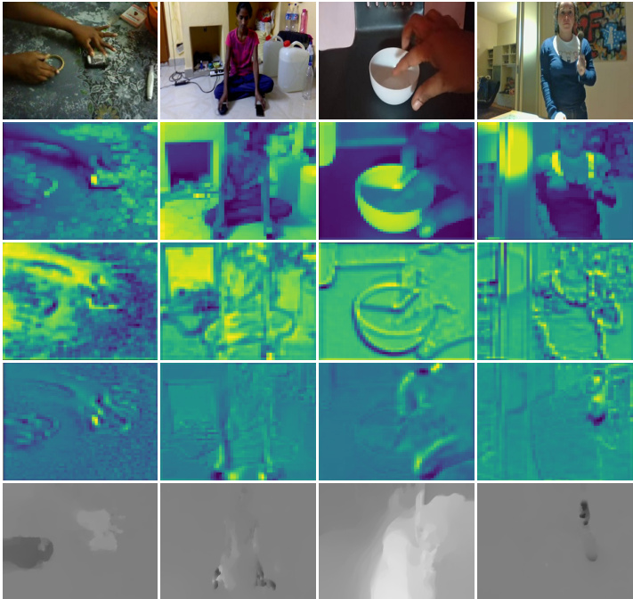
Figure 1. Feature visualization of STM block. First row is the input frames. Second row is the input feature maps of Conv2 1 block. Third row is the output s patio temporal feature maps of CSTM. The fourth row is the output motion feature maps of CMM. The last row is the optical flow extracted by TV-L1.
图 1: STM模块特征可视化。第一行为输入帧序列。第二行为Conv2_1模块的输入特征图。第三行为CSTM输出的时空特征图。第四行为CMM输出的运动特征图。最后一行是TV-L1算法提取的光流场。
The existing methods for action recognition can be summarized into two categories. The first type is based on twostream neural networks [10, 33, 36, 9], which consists of an RGB stream with RGB frames as input and a flow stream with optical flow as input. The spatial stream models the appearance features (not s patio temporal features) without considering the temporal information. The flow stream is usually called as a temporal stream, which is designed to model the temporal cues. However, we argue that it is inaccurate to refer the flow stream as the temporal stream because the optical flow only represent the motion features between the neighboring frames and the structure of this stream is almost the same to the spatial stream with 2D CNN. Therefore, this flow stream lacks of the ability to capture the long-range temporal relationship. Besides, the extraction of optical flow is expensive in both time and space, which limits vast industrial applications in the real world.
现有的动作识别方法可归纳为两类。第一类是基于双流神经网络 [10, 33, 36, 9] 的方法,包含以RGB帧为输入的RGB流和以光流为输入的光流流。空间流建模的是外观特征(而非时空特征),未考虑时序信息。光流流通常被称为时序流,旨在建模时序线索。但我们认为将光流流称为时序流并不准确,因为光流仅表征相邻帧间的运动特征,且该流的结构与采用2D CNN的空间流几乎相同。因此,这种光流流缺乏捕捉长程时序关系的能力。此外,光流提取在时间和空间上都代价高昂,限制了其在现实工业场景中的广泛应用。
The other category is the 3D convolutional networks (3D CNNs) based methods, which is designed to capture the s patio temporal features[27, 2, 24, 3]. 3D convolution is able to represent the temporal features as well as the spatial features together benefiting from the extended temporal dimension. With stacked 3D convolutions, 3D CNNs can capture long-range temporal relationship. Recently, the optimization of this framework with tremendous parameters becomes popular because of the release of large-scale video datasets such as Kinetics [2]. With the help of pre-training on large-scale video datasets, 3D CNN based methods have achieved superior performance to 2D CNN based methods. However, although 3D CNN can model s patio temporal information from RGB inputs directly, many methods [29, 2] still integrate an independent optical-flow motion stream to further improve the performance with motion features. Therefore, these two features are complementary to each other in action recognition. Nevertheless, expanding the convolution kernel from 2D to 3D and the two-stream structure will inevitably increase the computing cost by an order of magnitude, which limits its real applications.
另一类是基于3D卷积网络 (3D CNNs) 的方法,旨在捕获时空特征 [27, 2, 24, 3]。得益于扩展的时间维度,3D卷积能同时表征时空特征。通过堆叠3D卷积,3D CNN可捕获长程时序关系。随着Kinetics [2] 等大规模视频数据集的发布,这种海量参数框架的优化近期备受关注。借助大规模视频数据集预训练,基于3D CNN的方法已取得优于2D CNN方法的性能。但尽管3D CNN能直接从RGB输入建模时空信息,许多方法 [29, 2] 仍会整合独立的光流运动流,利用运动特征进一步提升性能。因此在行为识别中,这两种特征具有互补性。然而,将卷积核从2D扩展到3D以及双流结构,不可避免地会使计算成本增加一个数量级,限制了其实际应用。
Inspired by the above observation, we propose a simple yet effective method referred as STM network, to integrate both S patio Temporal and Motion features in a unified 2D CNN framework, without any 3D convolution and optical flow pre-calculation. Given an input feature map, we adopt a Channel-wise S patio temporal Module (CSTM) to present the s patio temporal features and a Channel-wise Motion Module (CMM) to encode the motion features. We also insert an identity mapping path to combine them together as a block named STM block. The STM blocks can be easily inserted into existing ResNet [13] architectures by replacing the original residual blocks to form the STM networks with negligible extra parameters. As shown in Fig. 1, we visualize our STM block with CSTM and CMM features. The CSTM has learned the s patio temporal features which pay more attention on the main object parts of the action interaction compared to the original input features. As for the CMM, it captures the motion features with the distinct edges just like optical flow. The main contributions of our work can be summarized as follows:
受上述观察启发,我们提出了一种简单而有效的方法——STM网络(Spatio Temporal and Motion network),在统一的2D CNN框架中整合时空特征和运动特征,无需任何3D卷积或光流预计算。给定输入特征图时,我们采用通道级时空模块(CSTM)来呈现时空特征,并通过通道级运动模块(CMM)编码运动特征。同时引入恒等映射路径将它们组合为STM块。通过替换原始残差块,STM块可轻松嵌入现有ResNet [13]架构,形成几乎不增加参数的STM网络。如图1所示,我们可视化展示了具有CSTM和CMM特征的STM块。相较于原始输入特征,CSTM学习到的时空特征更关注动作交互的主体部位;而CMM则捕获了类似光流的清晰边缘运动特征。本研究的主要贡献可概括如下:
• We propose a Channel-wise S patio temporal Module (CSTM) and a Channel-wise Motion Module (CMM) to encode the complementary s patio temporal and motion features in a unified 2D CNN framework.
• 我们提出了通道级时空模块 (Channel-wise Spatio-temporal Module, CSTM) 和通道级运动模块 (Channel-wise Motion Module, CMM) ,用于在统一的2D CNN框架中编码互补的时空特征与运动特征。
A simple yet effective network referred as STM Network is proposed with our STM blocks, which can be inserted into existing ResNet architecture by introducing very limited extra computation cost. Extensive experiments demonstrate that by integrating both s patio temporal and motion features together, our method outperforms the state-of-the-art methods on several public benchmark datasets including Something-Something[11], Kinetics [2], Jester [1], UCF101 [23] and HMDB-51 [17].
我们提出了一种简单高效的STM网络,通过STM模块可嵌入现有ResNet架构,仅需引入极少量额外计算成本。大量实验表明,该方法通过融合时空特征与运动特征,在多个公开基准数据集上超越了当前最优方法,包括Something-Something[11]、Kinetics[2]、Jester[1]、UCF101[23]和HMDB-51[17]。
2. Related Works
2. 相关工作
With the great success of deep convolution networks in the computer vision area, a large number of CNN-based methods have been proposed for action recognition and have gradually surpassed the performance of traditional methods [30, 31]. A sequence of advances adopt 2D CNNs as the backbone and classify a video by simply aggregating frame-wise prediction [16]. However, these methods only model the appearance feature of each frame independently while ignore the dynamics between frames, which results in inferior performance when recognizing temporal-related videos. To handle the mentioned drawback, two-stream based methods [10, 33, 36, 3, 9] are introduced by modeling appearance and dynamics separately with two networks and fuse two streams through middle or at last. Among these methods, Simonyan et al. [22] first proposed the two-stream ConvNet architecture with both spatial and temporal networks. Temporal Segment Networks (TSN) [33] proposed a sparse temporal sampling strategy for the two-stream structure and fused the two streams by a weighted average at the end. Fei chten hofer et al. [8, 9] studied the fusion strategies in the middle of the two streams in order to obtain the s patio temporal features. However, these types of methods mainly suffer from two limitations. First, these methods need pre-compute optical flow, which is expensive in both time and space. Second, the learned feature and final prediction from multiple segments are fused simply using weighted or average sum, making it inferior to temporalrelationship modeling.
随着深度卷积网络在计算机视觉领域的巨大成功,大量基于CNN的方法被提出用于动作识别,并逐渐超越传统方法的性能[30, 31]。一系列研究采用2D CNN作为主干网络,通过简单聚合逐帧预测结果对视频进行分类[16]。然而,这些方法仅独立建模每帧的表观特征,而忽略了帧间动态关系,导致在识别时序相关视频时性能欠佳。
为克服上述缺陷,基于双流的方法[10, 33, 36, 3, 9]被提出,通过两个网络分别建模表观特征和动态特征,并在中间或最后阶段融合双流信息。其中,Simonyan等人[22]首次提出包含空间网络和时间网络的双流ConvNet架构。时序分段网络(TSN)[33]为双流结构设计了稀疏时序采样策略,最终通过加权平均融合双流。Feichtenhofer等人[8, 9]研究了双流中间阶段的融合策略,以获取时空联合特征。
但这类方法存在两个主要局限:首先需要预先计算光流,时空开销较大;其次多片段学习特征与最终预测仅通过加权或平均求和简单融合,导致时序关系建模能力不足。
Another type of methods tries to learn s patio temporal features from RGB frames directly with 3D CNN [27, 2, 4, 7, 24]. C3D [27] is the first work to learn s patio temporal features using deep 3D CNN. However, with tremendous parameters to be optimized and lack of high-quality largescale datasets, the performance of C3D remains unsatisfactory. I3D [2] inflated the ImageNet pre-trained 2D kernel into 3D to capture s patio temporal features and modeled motion features with another flow stream. I3D has achieved very competitive performance in benchmark datasets with the help of high-quality large-scale Kinetics dataset and the two-stream setting. Since 3D CNNs try to learn local correlation along the input channels, STCNet [4] inserted its STC block into 3D ResNet to captures both spatial-channels and temporal-channels correlation information throughout network layers. Slowfast [7] involved a slow path to capture spatial semantics and a fast path to capture motion at fine temporal resolution. Although 3D CNN based methods have achieved state-of-the-art performance, they still suffer from heavy computation, making it hard to deploy in realworld applications.
另一类方法尝试直接用3D CNN从RGB帧中学习时空特征[27, 2, 4, 7, 24]。C3D[27]是首个使用深度3D CNN学习时空特征的工作。但由于需要优化的参数量巨大且缺乏高质量大规模数据集,C3D的性能仍不尽如人意。I3D[2]将ImageNet预训练的2D核膨胀为3D以捕获时空特征,并通过另一个光流流建模运动特征。借助高质量的大规模Kinetics数据集和双流设置,I3D在基准数据集上取得了极具竞争力的性能。由于3D CNN试图学习输入通道间的局部相关性,STCNet[4]将其STC模块插入3D ResNet,在整个网络层中捕获空间-通道和时间-通道的关联信息。Slowfast[7]采用慢路径捕获空间语义,快路径以精细时间分辨率捕获运动。虽然基于3D CNN的方法已取得最先进性能,但仍受困于沉重计算量,难以在实际应用中部署。
To handle the heavy computation of 3D CNNs, several methods are proposed to find the trade-off between precision and speed [28, 37, 42, 41, 25, 20]. Tran et al. [28] and Xie et al. [37] discussed several forms of spatiotemporal convolutions including employing 3D convolution in early layers and 2D convolution in deeper layers (bottomheavy) or reversed the combinations (top-heavy). P3D [20] and $_{\mathrm{R}(2+1)\mathrm{D}}$ [28] tried to reduce the cost of 3D convolution by decomposing it into 2D spatial convolution and 1D temporal convolution. TSM [19] further introduced the temporal convolution by shifting part of the channels along the temporal dimension. Our proposed CSTM branch is similar to these methods in the mean of learning s patio temporal features, while we employ channel-wise 1D convolution to capture different temporal relationship for different channels. Though these methods are successful in balancing the heavy computation of 3D CNNs, they inevitably need the help of two-stream networks with a flow stream to incorporate the motion features to obtain their best performance. Motion information is the key difference between video-based recognition and image-based recognition task. However, calculating optical flow with TV-L1 method [38] is expensive in both time and space. Recently many approaches have been proposed to estimate optical flow with CNN [5, 14, 6, 21] or explored alternatives of optical flow [33, 39, 26, 18]. TSN frameworks [33] involved RGB difference between two frames to represent motion in videos. Zhao et al. [39] used cost volume processing to model apparent motion. Optical Flow guided Feature (OFF) [26] contains a set of operators including sobel and element-wise subtraction for OFF generation. MFNet [18] adopted five fixed motion filters as a motion block to find feature-level temporal features between two adjacent time steps. Our proposed CMM branch is also designed for finding better yet lightweight alternative motion representation. The main difference is that we learn different motion features for different channels for every two adjacent time steps.
为应对3D CNN的高计算量,研究者们提出了多种精度与速度的平衡方案[28, 37, 42, 41, 25, 20]。Tran等[28]与Xie等[37]探讨了时空卷积的多种形式,包括在浅层使用3D卷积而深层使用2D卷积(底部密集型)或其反向组合(顶部密集型)。P3D[20]与$_{\mathrm{R}(2+1)\mathrm{D}}$[28]通过将3D卷积分解为2D空间卷积与1D时序卷积来降低计算成本。TSM[19]进一步通过沿时间维度偏移部分通道来引入时序卷积。我们提出的CSTM分支在学习时空特征方面与这些方法类似,但采用通道级1D卷积来捕捉不同通道的时序关系。尽管这些方法成功平衡了3D CNN的计算负担,它们仍需依赖双流网络中的光流支路来融合运动特征以获得最佳性能。
运动信息是视频识别与图像识别任务的关键差异。然而,基于TV-L1方法[38]的光流计算在时间和空间上代价高昂。近期研究提出了多种基于CNN的光流估计方法[5, 14, 6, 21]或光流替代方案[33, 39, 26, 18]。TSN框架[33]采用帧间RGB差值表示视频运动。Zhao等[39]使用代价体积处理建模表观运动。光流引导特征(OFF)[26]包含sobel算子与逐元素减法等操作符来生成运动特征。MFNet[18]采用五个固定运动滤波器作为运动块来提取相邻时间步的特征级时序特征。我们提出的CMM分支同样致力于寻找更轻量级的运动表征替代方案,核心区别在于我们为每对相邻时间步的不同通道学习差异化运动特征。
3. Approach
3. 方法
In this section, we will introduce the technical details of our approach. First, we will describe the proposed CSTM and CMM to show how to perform the channel-wise spatio temporal fusion and extract the feature-level motion information, respectively. Afterward, we will present the combination of these two modules to assemble them as a building block that can be inserted into existing ResNet architecture to form our STM network.
在本节中,我们将介绍方法的技术细节。首先,我们将描述提出的CSTM和CMM,分别展示如何进行通道级时空融合和提取特征级运动信息。随后,我们将介绍这两个模块的组合方式,将其构建为可插入现有ResNet架构的基础模块,从而形成我们的STM网络。
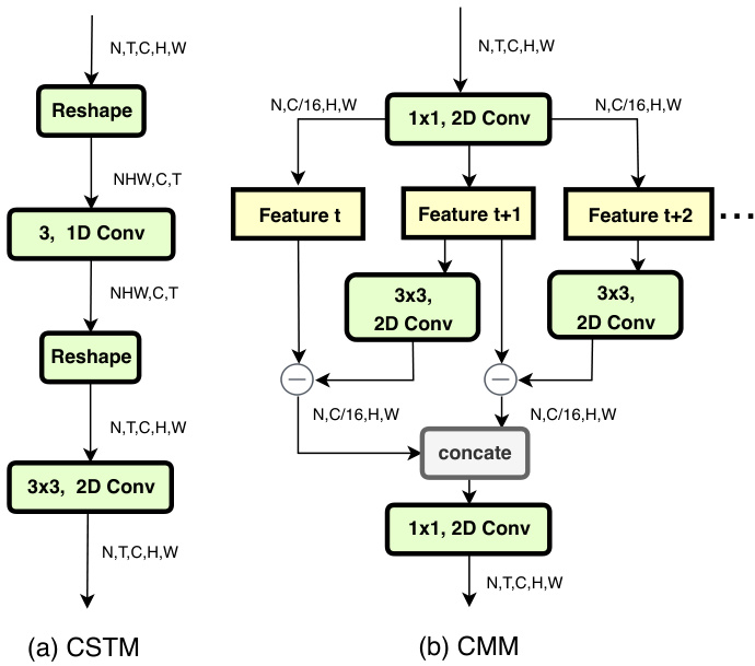
Figure 2. Architecture of Channel-wise S patio Temporal Module and Channel-wise Motion Module. The feature maps are shown as the shape of their tensors. ” $\ominus$ ” denotes element-wise subtraction.
图 2: 通道级时空模块 (Channel-wise Spatio Temporal Module) 和通道级运动模块 (Channel-wise Motion Module) 的架构。特征图以张量形状表示。"$\ominus$"表示逐元素减法。
3.1. Channel-wise S patio Temporal Module
3.1. 通道级时空模块
The CSTM is designed for efficient spatial and temporal modeling. By introducing very limited extra computing cost, CSTM extracts rich s patio temporal features, which can significantly boost the performance of temporal-related action recognition. As illustrated in Fig. 2(a), given an input feature map $\mathbf{F}\in\mathbb{R}^{N\times T\times C\times H\times W}$ , we first reshape $\mathbf{F}$ as: $\mathbf{F}\rightarrow\mathbf{F^{}}\in\mathbb{R}^{N H W\times C\times T}$ and then apply the channelwise 1D convolution on the $T$ dimension to fuse the temporal information. There are mainly two advantages to adopt the channel-wise convolution rather than the ordinary convolution. Firstly, for the feature map $\mathbf{F}^{*}$ , the semantic information of different channels is typically different. We claim that the combination of temporal information for different channels should be different. Thus the channel-wise convolution is adopted to learn independent kernels for each channel. Secondly, compared to the ordinary convolution, the computation cost can be reduced by a factor of $G$ where $G$ is the number of groups. In our settings, $G$ is equal to the number of input channels. Formally, the channel-wise temporal fusion operation can be formulated as:
CSTM专为高效的空间和时间建模而设计。通过引入非常有限的额外计算成本,CSTM提取了丰富的时空特征,可显著提升时间相关动作识别的性能。如图 2(a) 所示,给定输入特征图 $\mathbf{F}\in\mathbb{R}^{N\times T\times C\times H\times W}$,我们首先将 $\mathbf{F}$ 重塑为:$\mathbf{F}\rightarrow\mathbf{F^{}}\in\mathbb{R}^{N H W\times C\times T}$,然后在 $T$ 维度上应用通道级一维卷积来融合时间信息。采用通道级卷积而非普通卷积主要有两个优势。首先,对于特征图 $\mathbf{F}^{*}$,不同通道的语义信息通常不同。我们认为不同通道的时间信息组合应当有所区别,因此采用通道级卷积为每个通道学习独立的核。其次,与普通卷积相比,计算成本可降低 $G$ 倍,其中 $G$ 为分组数。在我们的设置中,$G$ 等于输入通道数。形式上,通道级时间融合操作可表述为:
$$
\mathbf{G}{c,t}=\sum_{i}\mathbf{K}{i}^{c}\mathbf{F}_{c,t+i}^{*}
$$
$$
\mathbf{G}{c,t}=\sum_{i}\mathbf{K}{i}^{c}\mathbf{F}_{c,t+i}^{*}
$$
where $\mathbf{K}{i}^{c}$ are temporal combination kernel weights belong to channel c and i is the index of temporal kernel, F*,t+i is the input feature sequence and $\mathbf{G}_{c,t}$ is the updated version of the channel-wise temporal fusion features. Here the temporal kernel size is set to 3 thus $i\in[-1,1]$ . Next we will reshape the $\mathbf{G}$ to the original input shape (i.e. $[N,T,C,H,W])$ and model local-spatial information via 2D convolution whose kernel size is $3\mathrm{x}3$ .
其中 $\mathbf{K}{i}^{c}$ 是属于通道 c 的时间组合核权重,i 是时间核的索引,F*,t+i 是输入特征序列,$\mathbf{G}_{c,t}$ 是通道级时间融合特征的更新版本。此处时间核大小设为 3,因此 $i\in[-1,1]$。接下来我们将 $\mathbf{G}$ 重塑为原始输入形状 (即 $[N,T,C,H,W]$),并通过核大小为 $3\mathrm{x}3$ 的 2D 卷积建模局部空间信息。
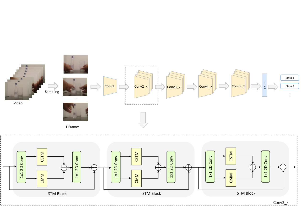
Figure 3. The overall architecture of STM network. The input video is first split into $N$ segments equally and then one frame from each segment is sampled. We adopt 2D ResNet-50 as backbone and replace all residual blocks with STM blocks. No temporal dimension reduction performed apart from the last score fusion stage.
图 3: STM网络的整体架构。输入视频首先被均匀分割为$N$个片段,然后从每个片段中采样一帧。我们采用2D ResNet-50作为主干网络,并将所有残差块替换为STM块。除最后的分数融合阶段外,未进行任何时间维度压缩。
We visualize the output feature maps of CSTM to help understand this module in Fig. 1. Compare the features in the second row to the third row, we can find that the CSTM has learned the s patio temporal features which pay more attention in the main part of the actions such as the hands in the first column while the background features are weak.
我们在图 1 中可视化 CSTM 的输出特征图以帮助理解该模块。将第二行与第三行的特征进行比较,可以发现 CSTM 学习到的时空特征更关注动作的主要部分 (如第一列中的手部动作) ,而背景特征较弱。
3.2. Channel-wise Motion Module
3.2. 通道级运动模块
As discovered in [29, 2], apart from the s patio temporal features directly learned by 3D CNN from the RGB stream, the performance can still be greatly improved by including an optical-flow motion stream. Therefore, apart from the CSTM, we propose a lightweight Channel-wise Motion Module (CMM) to extract feature-level motion patterns between adjacent frames. Note that our aim is to find the motion representation that can help to recognize actions in an efficient way rather than accurate motion information (optical flow) between two frames. Therefore, we will only use the RGB frames and not involve any pre-computed optical flow.
如[29, 2]所述,除了3D CNN直接从RGB流中学习的时空特征外,加入光流运动流仍能大幅提升性能。因此,我们在CSTM之外提出了轻量级的通道运动模块(CMM)来提取相邻帧间的特征级运动模式。需注意的是,我们的目标是寻找能高效辅助动作识别的运动表征,而非两帧间精确的运动信息(光流)。因此,我们将仅使用RGB帧而不涉及任何预计算光流。
Given the input feature maps $\mathbf{F}\in\mathbb{R}^{N\times T\times C\times H\times W}$ , we will first leverage a 1x1 convolution layer to reduce the spatial channels by a factor of $r$ to ease the computing cost, which is setting to 16 in our experiments. Then we generate feature-level motion information from every two consecutive feature maps. Taking $\mathbf{F}{t}$ and $\mathbf{F}{t+1}$ for example, we first apply 2D channel-wise convolution to $\mathbf{F}{t+1}$ and then subtracts from $\mathbf{F}{t}$ to obtain the approximate motion representation $\mathbf{H}_{t}$ :
给定输入特征图 $\mathbf{F}\in\mathbb{R}^{N\times T\times C\times H\times W}$ ,我们首先利用1x1卷积层将空间通道数缩减为原来的 $1/r$ 以降低计算成本(实验中设为16)。随后从每两个连续特征图中提取特征级运动信息。以 $\mathbf{F}{t}$ 和 $\mathbf{F}{t+1}$ 为例,先对 $\mathbf{F}{t+1}$ 进行二维通道卷积操作,再与 $\mathbf{F}{t}$ 相减得到近似运动表征 $\mathbf{H}_{t}$ :
$$
\mathbf{H}{t}=\sum_{i,j}\mathbf{K}{i,j}^{c}\mathbf{F}{t+1,c,h+i,w+j}-\mathbf{F}_{t}
$$
$$
\mathbf{H}{t}=\sum_{i,j}\mathbf{K}{i,j}^{c}\mathbf{F}{t+1,c,h+i,w+j}-\mathbf{F}_{t}
$$
where $c,t,h,w$ denote spatial, temporal channel and two spatial dimensions of the feature map respectively and $\mathbf{K}_{i,j}^{c}$ denotes the $c$ -th motion filter with the subscripts $i,j$ denote the spatial indices of the kernel. Here the kernel size is set to $3\times3$ thus $i,j\in[-1,1]$ .
其中 $c,t,h,w$ 分别表示特征图的空间、时间通道和两个空间维度,$\mathbf{K}_{i,j}^{c}$ 表示第 $c$ 个运动滤波器,下标 $i,j$ 表示核的空间索引。这里核大小设为 $3\times3$,因此 $i,j\in[-1,1]$。
As shown in Fig. 2(b), we perform the proposed CMM to every two adjacent feature maps over the temporal dimension, i.e., $\mathbf{F_{t}$ and $\mathbf{F}{t+1}$ , $\mathbf{F}{t+1}$ and $\mathbf{F}_{t+2}$ , etc. Therefore, the CMM will produce $T-1$ motion representations. To keep the temporal size compatible with the input feature maps, we simply use zero to represent the motion information of the last time step and then concatenate them together over the temporal dimension. In the end, another 1x1 2D convolution layer is applied to restore the number of channels to $C$ .
如图 2(b)所示,我们对时间维度上每两个相邻的特征图(即 $\mathbf{F}{t}$ 和 $\mathbf{F}{t+1}$ 、 $\mathbf{F}{t+1}$ 和 $\mathbf{F}_{t+2}$ 等)执行提出的 CMM 方法。因此,CMM 将生成 $T-1$ 个运动表征。为保持时间维度与输入特征图兼容,我们简单地用零表示最后一个时间步的运动信息,然后在时间维度上将其拼接起来。最后,再应用一个 1x1 2D 卷积层将通道数恢复至 $C$ 。
We find that the proposed CMM can boost the performance of the whole model even though the design is quite simple, which proves that the motion features obtained with CMM are complementary to the s patio temporal features from CSTM. We visualize the motion features learned by CMM in Fig. 1. From which we can see that compared to the output of CSTM, CMM is able to capture the motion features with the distinct edges just like optical flows.
我们发现,尽管设计相当简单,但所提出的CMM仍能提升整个模型的性能,这证明通过CMM获取的运动特征与来自CSTM的时空特征具有互补性。我们在图1中可视化了CMM学习到的运动特征。从中可以看出,与CSTM的输出相比,CMM能够像光流一样捕捉到具有清晰边缘的运动特征。
3.3. STM Network
3.3. STM网络
In order to keep the framework effective yet lightweight, we combine the proposed CSTM and CMM together to build an STM block that can encode s patio temporal and motion features together and can be easily inserted into the existing ResNet architectures. The overall design of the STM block is illustrated in the bottom half of Fig. 3. In this STM block, the first 1x1 2D convolution layer is responsible for reducing the channel dimensions. The compressed feature maps are then passed through the CSTM and CMM to extract s patio temporal and motion features respectively. Typically, there are two kinds of ways to aggregate different type of information: summation and concatenation. We experimentally found that summation works better than concatenation to fuse these two modules. Therefore, an elementwise sum operation is applied after the CSTM and CMM to aggregate the information. Then another 1x1 2D convolution layer is applied to restore the channel dimensions. Similar to the ordinary residual block, we also add a parameterfree identity shortcut from the input to the output.
为了保持框架高效且轻量,我们将提出的CSTM与CMM相结合,构建了一个能同时编码时空特征与运动特征的STM模块,该模块可轻松嵌入现有ResNet架构。STM模块的整体设计如图3下半部分所示:首先通过1x1二维卷积层降低通道维度,压缩后的特征图分别输入CSTM和CMM以提取时空特征与运动特征。信息聚合通常采用求和(summation)或拼接(concatenation)两种方式,实验表明求和操作能更有效融合这两个模块,因此在CSTM和CMM后采用逐元素求和进行特征聚合,再通过1x1二维卷积恢复通道维度。与常规残差块类似,我们在输入输出间添加了无参数的恒等捷径连接。
Because the proposed STM block is compatible with the ordinary residual block, we can simply insert it into any existing ResNet architectures to form our STM network with very limited extra computation cost. We illustrate the overall architecture of STM network in the top half of Figure 3. The STM network is a 2D convolutional network which avoids any 3D convolution and pre-computing optical flow. Unless specified, we choose the 2D ResNet-50 [13] as our backbone for its tradeoff between the accuracy and speed. We replace all residual blocks with the proposed STM blocks.
由于提出的STM模块与普通残差块兼容,我们可以轻松将其插入任何现有ResNet架构中,仅需极少额外计算成本即可构建STM网络。图3上半部分展示了STM网络的整体架构。该网络采用2D卷积结构,避免使用任何3D卷积和预计算光流。除非特别说明,我们选择2D ResNet-50 [13]作为主干网络以平衡精度与速度,并将所有残差块替换为提出的STM模块。
4. Experiments
4. 实验
In this section, we first introduce the datasets and the implementation details of our proposed approach. Then we perform extensive experiments to demonstrate that the proposed STM outperforms all the state-of-the-art methods on both temporal-related datasets (i.e., SomethingSomething v1 & v2 and Jester) and scene-related datasets (i.e., Kinetics-400, UCF-101, and HMDB-51). The baseline method in our experiments is Temporal Segment Networks (TSN) [33] where we replace the backbone to ResNet-50 for fair comparisons. We also conduct abundant ablation studies with Something-Something v1 to analyze the effectiveness of our method. Finally, we give runtime analyses to show the efficiency of STM compare with stateof-the-art methods.
在本节中,我们首先介绍数据集和所提出方法的实现细节。随后通过大量实验证明,提出的STM方法在时序相关数据集(即SomethingSomething v1 & v2和Jester)与场景相关数据集(即Kinetics-400、UCF-101和HMDB-51)上均优于所有最先进方法。实验中以时序分段网络(TSN)[33]为基线方法,为公平比较将其骨干网络替换为ResNet-50。我们还基于Something-Something v1数据集进行了充分的消融实验以分析方法的有效性。最后通过运行时分析展示了STM相比前沿方法的高效性。
4.1. Datasets
4.1. 数据集
We evaluate the performance of the proposed STM on several public action recognition datasets. We classify these datasets into two categories: (1) temporal-related datasets, including Something-Something v1 & v2 [11] and Jester [1]. For these datasets, temporal motion interaction of objects is the key to action understanding. Most of the actions cannot be recognized without considering the temporal relationship; (2) scene-related datasets, including Kinetics400 [2], UCF-101 [23] and HMDB-51 [17] where the background information contributes a lot for determining the action label in most of the videos. Temporal relation is not as important as it in the first group of datasets. We also give examples in Figure 4 to show the difference between them. Since our method is designed for effective s patio temporal fusion and motion information extraction, we mainly focus on those temporal-related datasets. Nevertheless, for those scene-related datasets, our method also achieves competitive results.
我们在多个公开动作识别数据集上评估了所提出的STM方法的性能。将这些数据集分为两类:(1) 时序相关数据集,包括Something-Something v1 & v2 [11]和Jester [1]。对于这些数据集,物体间的时序运动交互是动作理解的关键,大多数动作若不考虑时序关系就无法识别;(2) 场景相关数据集,包括Kinetics400 [2]、UCF-101 [23]和HMDB-51 [17],其中背景信息在多数视频中对动作标签的判断起重要作用,时序关系的重要性不如第一类数据集。图4展示了这两类数据集的差异示例。由于我们的方法专为有效的时空融合和运动信息提取而设计,因此主要关注时序相关数据集。尽管如此,在场景相关数据集上,我们的方法也取得了具有竞争力的结果。
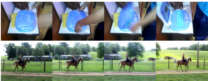
Figure 4. Difference between temporal-related datasets and scenerelated datasets. Top: action for which temporal feature matters. Reversing the order of frames gives the opposite label (opening something vs closing something). Bottom: action for which scene feature matters. Only one frame can predict label (horse riding).
图 4: 时序相关数据集与场景相关数据集的区别。上:时序特征起作用的动作。颠倒帧顺序会得到相反的标签(打开某物 vs 关闭某物)。下:场景特征起作用的动作。仅需一帧即可预测标签(骑马)。
4.2. Implementation Details
4.2. 实现细节
Training. We train our STM network with the same strategy as mentioned in TSN [33]. Given an input video, we first divide it into $T$ segments of equal durations in order to conduct long-range temporal structure modeling. Then, we randomly sample one frame from each segment to obtain the input sequence with $T$ frames. The size of the short side of these frames is fixed to 256. Meanwhile, corner cropping and scale-jittering are applied for data argumentation. Finally, we resize the cropped regions to $224\times224$ for network training. Therefore, the input size of the network is $N\times T\times3\times224\times224$ , where $N$ is the batch size and $T$ is the number of the sampled frames per video. In our experiments, $T$ is set to 8 or 16.
训练。我们采用与TSN [33]相同的策略训练STM网络。给定输入视频后,首先将其划分为$T$个等长片段以进行长程时序结构建模。随后从每个片段随机采样一帧,获得包含$T$帧的输入序列。这些帧的短边尺寸固定为256像素,同时采用角点裁剪和尺度抖动进行数据增强。最终将裁剪区域调整为$224\times224$分辨率用于网络训练,因此网络输入尺寸为$N\times T\times3\times224\times224$,其中$N$为批次大小,$T$为每视频采样帧数。实验中$T$设置为8或16。
We train our model with 8 GTX 1080TI GPUs and each GPU processes a mini-batch of 8 video clips (when $T=8$ ) or 4 video clips (when $T=16$ ). For Kinetics, SomethingSomething v1 & v2 and Jester, we start with a learning rate of 0.01 and reduce it by a factor of 10 at 30,40,45 epochs and stop at 50 epochs. For these large-scale datasets, we only use the ImageNet pre-trained model as initialization.
我们使用8块GTX 1080TI GPU训练模型,每块GPU处理8个视频片段的小批量(当$T=8$时)或4个视频片段(当$T=16$时)。对于Kinetics、SomethingSomething v1 & v2和Jester数据集,初始学习率为0.01,并在30、40、45个周期时降至十分之一,最终在50个周期停止训练。针对这些大规模数据集,我们仅采用ImageNet预训练模型进行初始化。
Table 1. Performance of the STM on the Something-Something v1 and v2 datasets compared with the state-of-the-art methods.
表 1: STM在Something-Something v1和v2数据集上的性能与最先进方法的对比
| 方法 | 骨干网络 | 光流 | 预训练 | 帧数 | Something-Somethingv1 | Something-Somethingv2 | |||||
|---|---|---|---|---|---|---|---|---|---|---|---|
| top-1 val | top-5 val | top-1 test | top-1 val | top-5 val | top-1 test | top-5 test | |||||
| S3D-G [37] | Inception | ImageNet | 64 | 48.2 | 78.7 | 42.0 | |||||
| ECO [42] | BNInception+ 3DResNet-18 | Kinetics | 8 | 39.6 41.4 | |||||||
| ECO [42] | 16 | 1 | 1 | ||||||||
| ECOEvLite[42] | 92 | 46.4 | 42.3 | ||||||||
| ECOEvLiteTwo-Stream[42] | 3DResNet-50 | Kinetics | 92+92 | 49.5 41.6 | 72.2 | 43.9 | - | - | |||
| I3D [2] | 32 32 | 43.4 | 1 | ||||||||
| I3D+GCN [2] | Kinetics | 8 | 19.7 | 75.1 46.6 | - | 27.8 | - | - | |||
| TSN [33] | ResNet-50 | 16 | 19.9 | 47.3 | 57.6 | ||||||
| - | 30.0 | 60.5 | |||||||||
| TRN Multiscale[40] | BNInception | ImageNet | 8 | 34.4 42.0 | 33.6 40.7 | 48.8 55.5 | 77.64 83.1 | 50.9 | 79.3 | ||
| TRN Two-Stream[40] MFNet-C101[18] | ResNet-101 | Scratch | 8+8 10 | 43.9 | 73.1 | 37.5 | - | 56.2 1 | 83.2 - | ||
| TSM [19] | ResNet-50 | Kinetics | 16 | 44.8 | 74.5 | 58.7 | 84.8 | 59.9 | 85.9 | ||
| TSM Two-Stream[19] | 16+8 | 49.6 | 79.0 | 46.1 | 63.5 | 88.6 | 63.7 | 89.5 | |||
| STM | ResNet-50 | ImageNet | 8 16 | 49.2 50.7 | 79.3 80.4 | 43.1 | 62.3 64.2 | 88.8 89.8 | 61.3 63.5 | 88.4 89.6 |
Table 2. Performance of the STM on the Jester compared with the state-of-the-art methods.
表 2: STM在Jester数据集上的性能与现有最优方法的对比。
| 方法 | 主干网络 | 帧数 | Top-1 | Top-5 |
|---|---|---|---|---|
| TSN [33] | ResNet-50 | 8 16 | 81.0 82.3 | 99.0 99.2 |
| TRN-Multiscale [40] | BNInception | 8 | 95.3 | |
| MFNet-C50 [18] | ResNet-50 | 7 | 96.1 | 99.7 |
| TSM [19] | ResNet-50 | 8 16 | 94.4 | 99.7 |
| STM | ResNet-50 | 8 16 | 95.3 96.6 96.7 | 99.8 99.9 99.9 |
For the temporal channel-wise 1D convolution in CSTM, first quarter of channels are initialized to [1,0,0], last quarter of channels are initialized to [0,0,1] and other half are [0,1,0]. All parameters in CMM are randomly initialized. For UCF-101 and HMDB-51, we use Kinetics pre-trained model as initialization and start training with a learning rate of 0.001 for 25 epochs. The learning rate is decayed by a factor 10 every 15 epochs. We use mini-batch SGD as optimizer with a momentum of 0.9 and a weight decay of 5e-4. Different from [33], we enable all the BatchNorm layers [15] during training.
对于CSTM中的时序通道一维卷积(1D convolution),前四分之一通道初始化为[1,0,0],后四分之一通道初始化为[0,0,1],其余半数通道初始化为[0,1,0]。CMM中所有参数均为随机初始化。在UCF-101和HMDB-51数据集上,我们采用Kinetics预训练模型进行初始化,以0.001的学习率训练25个周期,每15个周期学习率下降10倍。优化器采用小批量随机梯度下降(SGD),动量系数为0.9,权重衰减为5e-4。与[33]不同,我们在训练过程中启用了所有批归一化(BatchNorm)层[15]。
Inference. Following [34, 7], we first scale the shorter spatial side to 256 pixels and take three crops of $256\times256$ to cover the spatial dimensions and then resize them to $224\times224$ . For the temporal domain, we randomly sample 10 times from the full-length video and compute the softmax scores individually. The final prediction is the averaged softmax scores of all clips.
推理。参照 [34, 7],我们首先将较短的空间边缩放至 256 像素,并截取三个 $256\times256$ 的裁剪区域以覆盖空间维度,然后将它们调整为 $224\times224$。在时间域上,我们从完整视频中随机采样 10 次,并分别计算 softmax 分数。最终预测结果是所有片段的 softmax 分数的平均值。
4.3. Results on Temporal-Related Datasets
4.3. 时序相关数据集上的结果
In this section, we compare our approach with the stateof-the-art methods on temporal-related datasets including Something-Something v1 & v2 and Jester. SomethingSomething v1 is a large collection of densely-labeled video clips which shows basic human interactions with daily objects. This dataset contains 174 classes with 108,499 videos. Something-Something v2 is an updated version of v1 with more videos (220,847 in total) and greatly reduced label noise. Jester is a crowd-acted video dataset for generic human hand gestures recognition, which contains 27 classes with 148,092 videos.
在本节中,我们将我们的方法与包括Something-Something v1 & v2和Jester在内的时序相关数据集上的最先进方法进行比较。Something-Something v1是一个密集标注视频片段的大型集合,展示了人类与日常物品的基本互动。该数据集包含174个类别,共计108,499个视频。Something-Something v2是v1的更新版本,拥有更多视频(总计220,847个)并大幅减少了标签噪声。Jester是一个用于通用手势识别的众包视频数据集,包含27个类别,共计148,092个视频。
Table 3. Performance of the STM on the Kinetics-400 dataset compared with the state-of-the-art methods.
表 3: STM 在 Kinetics-400 数据集上的性能与最先进方法的对比。
| 方法 | 主干网络 | 光流 | Top-1 | Top-5 |
|---|---|---|---|---|
| STC [4] | ResNext101 | 68.7 | 88.5 | |
| ARTNet [32] | ResNet-18 | 69.2 | 88.3 | |
| ECO [42] | BNInception +3D ResNet-18 | 70.7 | 89.4 | |
| S3D [37] | Inception | 72.2 | 90.6 | |
| I3D RGB [2] | 3DInception-vl | 71.1 | 89.3 | |
| I3D Two-Stream [2] | 3DInception-vl | 74.2 | 91.3 | |
| StNet [12] | ResNet-101 | 71.4 | - | |
| Disentangling [39] | BNInception | 71.5 | 89.9 | |
| R(2+1)D RGB [28] | ResNet-34 | 72.0 | 90.0 | |
| R(2+1)D Two-Stream [28] | ResNet-34 | 73.9 | 90.9 | |
| TSM [19] | ResNet-50 | 72.5 | - | |
| TSN RGB [33] | BNInception | 69.1 | 88.7 | |
| TSN Two-Stream [33] | BNInception | 73.9 | 91.1 | |
| STM | ResNet-50 | 73.7 | 91.6 |
Table 1 lists the results of our method compared with the state-of-the-art on Something-Something v1 and v2. The results of the baseline method TSN are relatively low compared with other methods, which demonstrates the importance of temporal modeling for these temporal-related datasets. Compared with the baseline method, our STM network gains $29.5%$ and $30.8%$ top-1 accuracy improvement with 8 and 16 frames inputs respectively on SomethingSomething v1. On Something-Something v2, STM also gains $34.5%$ and $34.2%$ improvement compared to TSN. The rest part of Table 1 shows the other state-of-the-art methods. These methods can be classified into two types as shown in the two parts of Table 1. The upper part presents the 3D CNN based methods, including S3D-G [37], ECO [42] and $\mathrm{I}3\mathrm{D}{+}\mathrm{GCN}$ models [35]. The lower part is 2D CNN based methods, including TRN [40], MFNet [18] and TSM [19]. It is clear that even STM with 8 RGB frames as input achieves the state-of-the-art performance compared with other methods, which take more frames and optical flow as input or 3D CNN as the backbone. With 16 frames as input, STM achieves the best performance in the validation sets of both Something-Something v1 and v2, and just a little lower in the top1 accuracy in the test sets, which adopts only 16 RGB frames as input.
表 1: 列出了我们的方法与当前最先进方法在Something-Something v1和v2上的对比结果。基线方法TSN的性能相对其他方法较低,这证明了时序建模对这些时序相关数据集的重要性。与基线方法相比,我们的STM网络在Something-Something v1上分别以8帧和16帧输入获得了29.5%和30.8%的top-1准确率提升。在Something-Something v2上,STM相比TSN也分别实现了34.5%和34.2%的改进。表1其余部分展示了其他最先进方法,这些方法可分为两类:上半部分是基于3D CNN的方法(包括S3D-G [37]、ECO [42]和I3D+GCN模型 [35]),下半部分是基于2D CNN的方法(包括TRN [40]、MFNet [18]和TSM [19])。显然,即使仅使用8帧RGB输入,STM的性能也超越了其他需要更多帧数、光流输入或采用3D CNN主干网络的方法。当输入16帧时,STM在Something-Something v1和v2验证集上均取得最佳性能,在测试集top1准确率上仅略低(仅使用16帧RGB输入)。
Table 4. Performance of the STM on UCF-101 and HMDB-51 compared with the state-of-the-art methods.
表 4. STM 在 UCF-101 和 HMDB-51 上的性能与最先进方法的对比。
| 方法 | 骨干网络 | 光流 | 预训练数据 | UCF-101 | HMDB-51 |
|---|---|---|---|---|---|
| C3D [27] | 3D VGG-11 | Sports-1M | 82.3 | 51.6 | |
| STC [4] | ResNet101 | Kinetics | 93.7 | 66.8 | |
| ARTNet with TSN [32] | 3DResNet-18 | Kinetics | 94.3 | 70.9 | |
| ECO [42] | BNInception+3D ResNet-18 | Kinetics | 94.8 | 72.4 | |
| I3D RGB [2] I3D two-stream [2] | 3D Inception-v1 | √ | ImageNet+Kinetics | 95.1 98.0 | 74.3 80.7 |
| TSN [33] | ResNet-50 | ImageNet | 86.2 | 54.7 | |
| TSN RGB [33] TSN two-Stream [33] | BNInception | √ | ImageNet+Kinetics | 91.1 97.0 | - |
| TSM [19] | ResNet-50 | ImageNet+Kinetics | 94.5 | 70.7 | |
| StNet [12] | ResNet50 | ImageNet+Kinetics | 93.5 | 二 | |
| Disentangling [39] | BNInception | ImageNet+Kinetics | 95.9 | ||
| STM | ResNet-50 | ImageNet+Kinetics | 96.2 | 72.2 |
Table 2 shows the results on the Jester dataset. Our STM also gains a large improvement compared to the TSN baseline method, and outperforms all the state-of-the-art methods.
表 2: 展示了在Jester数据集上的结果。我们的STM方法相比TSN基线方法取得了显著提升,并且超越了所有最先进方法。
4.4. Results on Scene-Related Datasets
4.4. 场景相关数据集上的结果
We evaluate our STM on three scene-related datasets: Kinetics-400, UCF-101, and HMDB-51 in this section. Kinetics-400 is a large-scale human action video dataset with 400 classes. It contains 236,763 clips for training and 19,095 clips for validation. UCF-101 is a relatively small dataset which contains 101 categories and 13,320 clips in total. HMDB-51 is also a small video dataset with 51 classes and 6766 labeled video clips. For UCF-101 and HMDB-51, we followed [33] to adopt the three training/testing splits for evaluation.
我们在三个场景相关数据集上评估了STM模型:Kinetics-400、UCF-101和HMDB-51。Kinetics-400是一个包含400个类别的大规模人类动作视频数据集,其中训练集包含236,763个视频片段,验证集包含19,095个片段。UCF-101是一个相对较小的数据集,包含101个类别共计13,320个视频片段。HMDB-51同样是一个小型视频数据集,包含51个类别和6,766个标注视频片段。对于UCF-101和HMDB-51,我们遵循[33]采用三个训练/测试划分进行评估。
Table 3 summaries the results of STM and other competing methods on the Kinetics-400 dataset. We train STM with 16 frames as input, and the same for evaluation. From the evaluation results, we can draw the following conclusions: (1) Different from the previous temporal-related datasets, most actions of Kinetics can be recognized by scene and objects even with one still frame of videos, therefore the baseline method without any temporal modeling can achieve acceptable accuracy; (2) Though our method is mainly focused on temporal-related actions recognition, STM still achieves very competitive results compare with the state-of-the-art methods. Top-1 accuracy of our method is only $0.5%$ lower than the two-stream I3D, which involves both 3D convolution and pre-computation optical flow. However, STM outperforms major recently proposed 3D CNN based methods (the upper part of the Table 3) as well as 2D CNN based methods (the lower part of the Table 3) and achieve the best top-5 accuracy compared with all the other method.
表 3 总结了 STM 和其他竞争方法在 Kinetics-400 数据集上的结果。我们使用 16 帧作为输入训练 STM,并在评估时采用相同设置。从评估结果可以得出以下结论:(1) 与之前的时间相关数据集不同,Kinetics 的大部分动作仅通过场景和物体即可识别(即使仅使用单帧视频),因此无需任何时间建模的基线方法也能达到可接受的准确率;(2) 尽管我们的方法主要关注时间相关动作识别,STM 仍与最先进方法相比取得了极具竞争力的结果。我们的方法在 Top-1 准确率上仅比采用 3D 卷积和预计算光流的两流 I3D 低 $0.5%$,但 STM 优于近期主流的基于 3D CNN 的方法(表 3 上半部分)和基于 2D CNN 的方法(表 3 下半部分),并且在与所有其他方法比较时取得了最佳的 Top-5 准确率。
We also conduct experiments on the UCF-101 and HMDB-51 to study the generalization ability of learned spatio temporal and motion representations. We evaluate our method over three splits and report the averaged results in Table 4. First, compared with the ImageNet pre-trained model, Kinetics pre-train can significantly improve the performance on small datasets. Then, compare with the stateof-the-art methods, only two methods, I3D two-stream and TSN two-Stream, performs a little better than ours while both of them utilize optical flow as their extra inputs. However, STM with 16 frames as inputs even outperforms I3D with RGB stream on UCF101, which also uses Kinetics as pre-train data but the 3D CNN leads to much higher computation cost than ours.
我们还在UCF-101和HMDB-51数据集上进行了实验,以研究所学时空表征和运动表征的泛化能力。我们在三个数据划分上评估了方法性能,表4展示了平均结果。首先,与ImageNet预训练模型相比,Kinetics预训练能显著提升小数据集上的性能。其次,与最先进方法相比,仅I3D双流和TSN双流两种方法表现略优于我们,而这两种方法都使用了光流作为额外输入。值得注意的是,仅用16帧作为输入的STM模型在UCF101上甚至超越了采用RGB流的I3D模型(两者均使用Kinetics预训练数据),但3D CNN的计算成本远高于我们的方法。
4.5. Ablation Studies
4.5. 消融实验
In this section, we comprehensively evaluate our proposed STM on Something-Something v1 dataset. All the ablation experiments in this section use 8 RGB frames as inputs.
在本节中,我们在Something-Something v1数据集上全面评估了提出的STM方法。本节所有消融实验均使用8帧RGB图像作为输入。
Impact of two modules. Our proposed two modules can be inserted into a standard ResNet architecture independently. To validate the contributions of each component in the STM block (i.e., CSTM and CMM), we compare the results of the individual module and the combination of both modules in Table 5. We can see that each component contributes to the proposed STM block. CSTM learns channel-wise temporal fusion and brings about $28%$ top-1 accuracy improvement compared to the baseline method TSN while CMM learns feature-level motion information and brings $24.4%$ top-1 accuracy improvement. When combining CSTM and CMM together, we can learn richer s patio temporal and motion features and achieve the best top-1 accuracy, especially, the gain over the baseline is $29.5%$ .
两个模块的影响。我们提出的两个模块可以独立插入标准ResNet架构。为验证STM块中各组件(即CSTM和CMM)的贡献,我们在表5中比较了单个模块与双模块组合的效果。可以看出每个组件都对STM块有贡献:CSTM通过学习通道级时序融合,相比基线方法TSN带来约28%的top-1准确率提升;CMM通过学习特征级运动信息,带来24.4%的top-1准确率提升。当组合使用CSTM和CMM时,我们能学习更丰富的时空运动特征,取得最佳top-1准确率(较基线提升29.5%)。
| 聚合方式 | Top-1 | Top-5 |
|---|---|---|
| TSN | 19.7 | 46.6 |
| 求和 | 49.2 | 79.3 |
| 拼接 | 41.8 | 73.2 |
Table 5. Impact of two mod- Table 6. Fusion of two modules: ules: Comparison between Summation fusion is better. CSTM, CMM and STM.
| 模型 | Top-1 | Top-5 |
|---|---|---|
| TSN | 19.7 | 46.6 |
| CSTM | 47.7 | 77.9 |
| CMM | 44.1 | 74.8 |
| STM | 49.2 | 79.3 |
表 5. 两个模块的影响: CSTM、CMM 和 STM 之间的比较。
表 6. 两个模块的融合: 求和融合效果更优。
| 类型 | 通道维度 (Channel-wise) | 常规 (Ordinary) |
|---|---|---|
| Top-1 准确率 | 47.7 | 46.9 |
| 参数量 | 23.88M | 27.64M |
| 计算量 (FLOPs) | 32.93G | 40.59G |
Table 7. Location and number Table 8. Type of temporal conof STM block: Deeper location volution in CSTM: Channeland more blocks yeild better per- wise temporal convolution yields formance. better performance.
表 7. STM模块的位置与数量: 更深层位置和更多模块能带来更好的性能
表 8. CSTM中的时序卷积类型: 通道级时序卷积能带来更好的性能
| Stage | STMBlocks | Top-1 | Top-5 |
|---|---|---|---|
| 2 | 1 | 38.7 | 70.1 |
| 3 | 1 | 40.6 | 71.6 |
| 4 | 1 | 41.5 | 72.6 |
| 5 | 1 | 41.5 | 71.8 |
| 2-5 | 4 | 47.9 | 78.1 |
| 2-5 | 16 | 49.2 | 79.3 |
Fusion of two modules. There are two ways to combine CSTM and CMM: element-wise summation and concatenation. The element-wise summation is parameter-free and easy to implement. For concatenation fusion, we first concatenate outputs of CSTM and CMM over the channel dimension, and the dimension of concatenate features is $2C$ . Then a 1x1 convolution is applied to reduce the channels to $C$ . We conduct the experiments to study the two fusion ways as shown in Table 6, though summation aggregation is simple, it still outperforms concatenation by $7.4%$ at top-1 accuracy and $6.1%$ at top-5 accuracy.
两个模块的融合。结合CSTM和CMM有两种方式:逐元素求和与拼接融合。逐元素求和无需参数且易于实现。对于拼接融合,我们首先在通道维度上拼接CSTM和CMM的输出,拼接特征的维度为$2C$,然后通过1x1卷积将通道数降至$C$。如表6所示,我们通过实验对比了两种融合方式:尽管求和聚合方式简单,但其top-1准确率仍比拼接融合高$7.4%$,top-5准确率高出$6.1%$。
Location and number of STM block. ResNet-50 architecture can be divided into 6 stages. We refer the conv $_{2.\mathrm{X}}$ to conv5 x as stage 2 to stage 5. The first four rows of Table 7 compare the performance of replacing only the first residual block with STM on different stages in ResNet-50, from stage 2 to stage 5, respectively. We conclude from the results that replacing only one residual block already yield significant performance improvement compared to the baseline TSN, which demonstrates the effectiveness of the proposed STM block. One may notice that replacing the STM block at latter stage (e.g., stage 5) yield better accuracy than early stage (e.g., stage 2). One possible reason is that temporal modeling is beneficial more with larger receptive fields which can capture holistic features. We then replace one block for each stage (i.e., replacing four blocks in all) and leads to better results. When replacing all original residual blocks with STM blocks (i.e., 16 blocks in all), our model achieves the best performance.
STM模块的位置与数量。ResNet-50架构可分为6个阶段,我们将conv$_{2.\mathrm{X}}$至conv5_x分别称为阶段2至阶段5。表7前四行比较了在ResNet-50中分别替换阶段2至阶段5的首个残差块为STM模块的性能表现。结果表明:仅替换一个残差块相比基线TSN已带来显著性能提升,验证了STM模块的有效性。值得注意的是,在后阶段(如阶段5)替换STM模块比前阶段(如阶段2)能获得更高精度,可能原因是时序建模在更大感受野下更有利于捕获整体特征。随后我们在每个阶段各替换一个模块(共替换4个),获得了更好结果。当将所有原始残差块替换为STM模块(共16个)时,模型达到最佳性能。
Type of temporal convolution in CSTM. We choose channel-wise temporal convolution in CSTM to learn temporal combination individually for each channel. We also make comparison with ordinary temporal convolution in CSTM module and the result is shown in Table 8. With channel-wise convolution, we can achieve better performance with few parameters and FLOPs.
CSTM中的时序卷积类型。我们选择在CSTM中使用逐通道时序卷积 (channel-wise temporal convolution) 来独立学习每个通道的时间组合。我们还与CSTM模块中的普通时序卷积进行了比较,结果如表8所示。通过逐通道卷积,我们能够以较少的参数量和FLOPs实现更好的性能。
4.6. Runtime Analysis
4.6. 运行时分析
Our STM achieves the new state-of-the-art results on several benchmark datasets compared with other methods.
我们的STM在多个基准数据集上相比其他方法取得了最新的最优结果。
Table 9. Accuracy and model complexity of STM and other stateof-the-art methods on Something-Something V1 dataset. Single crop STM beats all competing methods with 62 videos per second with 8 frames as input. Measured on a single NVIDIA GTX 1080TI GPU.
表 9. STM 与其他先进方法在 Something-Something V1 数据集上的准确率和模型复杂度对比。单次裁剪 STM 以每秒 62 帧视频的速度(输入为 8 帧)击败所有竞争方法。测试环境为单块 NVIDIA GTX 1080TI GPU。
| 模型 | 帧数 | FLOPs | 参数量 | 速度 | 准确率 |
|---|---|---|---|---|---|
| I3D [2] | 64 | 306G | 28.0M | 6.4 V/s | 41.6 |
| ECO [42] | 16 | 64G | 47.5M | 46.3V/s | 41.4 |
| TSM [19] | 8 | 32.9G | 23.9M | 80.4V/s | 43.8 |
| 16 | 65.8G | 40.6V/s | 44.8 | ||
| STM | 8 | 33.3G | 24.0M | 62.0V/s | 47.5 |
| 16 | 66.5G | 32.0 V/s | 49.8 |
More importantly, it is a unified 2D CNN framework without any time-consuming 3D convolution and optical flow calculations. Table 9 shows the accuracy and model complexity of STM and several state-of-the-art methods on Something-Something v1 dataset. All evaluations are running on one GTX 1080TI GPU. For a fair comparison, we evaluate our method by evenly sampling 8 or 16 frames from a video and then apply the center crop. To evaluate speed, we use a batch size of 16 and ignore the time of data loading. Compared to I3D and ECO, STM achieves approximately $10\mathrm{x}$ and 2x less FLOPs (33.3G vs 306G, 64G) while $5.9%$ and $6.1%$ higher accuracy. Compared to $\mathrm{TSM}{\mathrm{16F}}$ , our $\mathrm{STM}_{8\mathrm{F}}$ gains $2.7%$ higher accuracy with $1.5\mathrm{x}$ faster speed and half FLOPs.
更重要的是,这是一个统一的二维卷积神经网络(2D CNN)框架,无需任何耗时的三维卷积和光流计算。表9展示了STM及多种前沿方法在Something-Something v1数据集上的准确率与模型复杂度。所有评估均在单块GTX 1080TI GPU上运行。为公平对比,我们采用均匀采样8或16帧视频片段并中心裁剪的评估方式。测速时使用批处理量16且不计入数据加载时间。相比I3D和ECO,STM在减少约10倍和2倍浮点运算量(33.3G vs 306G, 64G)的同时,准确率分别提升5.9%和6.1%。与TSM₁₆F相比,我们的STM₈F以1.5倍速度和半数运算量实现了2.7%的准确率优势。
5. Conclusion
5. 结论
In this paper, we presented a simple yet effective network for action recognition by encoding s patio temporal and motion features together in a unified 2D CNN network. We replace the original residual blocks with STM blocks in ResNet architecture to build the STM network. An STM block contains a CSTM to model channel-wise spatio temporal feature and a CMM to model channel-wise mo- tion representation together. Without any 3D convolution and pre-calculation optical flow, our STM receives state-ofthe-art results on both temporal-related datasets and scenerelated datasets with only $1.2%$ more FLOPs compared to TSN baseline.
本文提出了一种简单而有效的动作识别网络,通过在统一的2D CNN网络中共同编码时空和运动特征。我们在ResNet架构中用STM块替换原始残差块来构建STM网络。STM块包含一个用于建模通道级时空特征的CSTM和一个用于共同建模通道级运动表征的CMM。在不使用任何3D卷积和预计算光流的情况下,我们的STM在时序相关数据集和场景相关数据集上均取得了最先进的结果,仅比TSN基线多消耗1.2%的FLOPs。
References
参考文献
Computer Vision and Pattern Recognition, pages 449–458, 2018. [42] Mohammad reza Zolfaghari, Kamaljeet Singh, and Thomas Brox. Eco: Efficient convolutional network for online video understanding. In Proceedings of the European Conference on Computer Vision (ECCV), pages 695–712, 2018.
计算机视觉与模式识别,第449-458页,2018年。[42] Mohammad reza Zolfaghari, Kamaljeet Singh 和 Thomas Brox。ECO:面向在线视频理解的高效卷积网络。载于欧洲计算机视觉会议(ECCV)论文集,第695-712页,2018年。