End-to-End Object Detection with Transformers
基于Transformer的端到端目标检测
Nicolas Carion $\star$ , Francisco Massa $\star$ , Gabriel Synnaeve, Nicolas Usunier, Alexander Kirillov, and Sergey Zagoruyko
Nicolas Carion $\star$、Francisco Massa $\star$、Gabriel Synnaeve、Nicolas Usunier、Alexander Kirillov 和 Sergey Zagoruyko
Facebook AI
Facebook AI
Abstract. We present a new method that views object detection as a direct set prediction problem. Our approach streamlines the detection pipeline, effectively removing the need for many hand-designed components like a non-maximum suppression procedure or anchor generation that explicitly encode our prior knowledge about the task. The main ingredients of the new framework, called DEtection TRansformer or DETR, are a set-based global loss that forces unique predictions via bipartite matching, and a transformer encoder-decoder architecture. Given a fixed small set of learned object queries, DETR reasons about the relations of the objects and the global image context to directly output the final set of predictions in parallel. The new model is conceptually simple and does not require a specialized library, unlike many other modern detectors. DETR demonstrates accuracy and run-time performance on par with the well-established and highly-optimized Faster RCNN baseline on the challenging COCO object detection dataset. Moreover, DETR can be easily generalized to produce panoptic segmentation in a unified manner. We show that it significantly outperforms competitive baselines. Training code and pretrained models are available at https://github.com/facebook research/detr.
摘要。我们提出了一种将目标检测视为直接集合预测问题的新方法。该方法简化了检测流程,有效消除了对非极大值抑制或锚框生成等人工设计组件的依赖,这些组件显式编码了我们对任务的先验知识。新框架DEtection TRansformer (DETR)的核心要素包括:基于集合的全局损失函数(通过二分匹配强制实现唯一预测)和Transformer编码器-解码器架构。给定一组固定的学习对象查询,DETR通过分析对象间关系及全局图像上下文,直接并行输出最终的预测集合。与许多现代检测器不同,该新模型概念简洁且无需专用库支持。在具有挑战性的COCO目标检测数据集上,DETR的准确率和运行时性能与经过高度优化的Faster RCNN基准相当。此外,DETR能统一泛化至全景分割任务,实验表明其显著优于竞争基线。训练代码与预训练模型详见https://github.com/facebookresearch/detr。
1 Introduction
1 引言
The goal of object detection is to predict a set of bounding boxes and category labels for each object of interest. Modern detectors address this set prediction task in an indirect way, by defining surrogate regression and classification problems on a large set of proposals [37,5], anchors [23], or window centers [53,46]. Their performances are significantly influenced by post processing steps to collapse near-duplicate predictions, by the design of the anchor sets and by the heuristics that assign target boxes to anchors [52]. To simplify these pipelines, we propose a direct set prediction approach to bypass the surrogate tasks. This end-to-end philosophy has led to significant advances in complex structured prediction tasks such as machine translation or speech recognition, but not yet in object detection: previous attempts [43,16,4,39] either add other forms of prior knowledge, or have not proven to be competitive with strong baselines on challenging benchmarks. This paper aims to bridge this gap.
目标检测的目标是预测一组边界框和每个感兴趣对象的类别标签。现代检测器通过在大规模候选框[37,5]、锚点[23]或窗口中心[53,46]上定义替代回归和分类问题,以间接方式解决这一集合预测任务。它们的性能受到后处理步骤(用于消除近似重复预测)、锚点集设计以及将目标框分配给锚点的启发式方法[52]的显著影响。为了简化这些流程,我们提出了一种直接集合预测方法以绕过替代任务。这种端到端的理念已在机器翻译或语音识别等复杂结构化预测任务中取得重大进展,但在目标检测领域尚未实现:先前尝试[43,16,4,39]要么引入了其他形式的先验知识,要么未能在具有挑战性的基准测试中证明其与强基线模型的竞争力。本文旨在弥合这一差距。
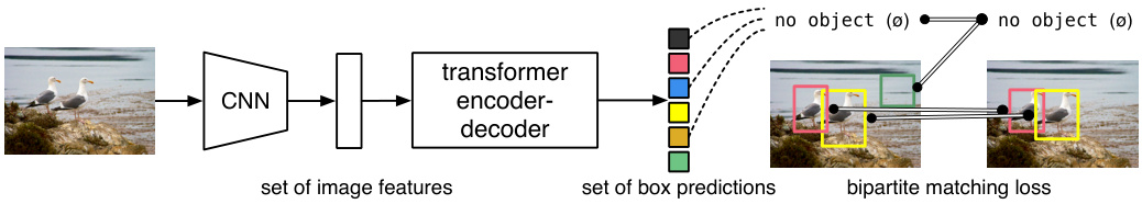
Fig. 1: DETR directly predicts (in parallel) the final set of detections by combining a common CNN with a transformer architecture. During training, bipartite matching uniquely assigns predictions with ground truth boxes. Prediction with no match should yield a “no object” $(\emptyset)$ class prediction.
图 1: DETR通过将普通CNN与Transformer架构相结合,直接(并行)预测最终的检测结果集。训练期间,二分匹配将预测结果与真实标注框唯一对应。未匹配的预测应产生"无物体" $(\emptyset)$ 类别预测。
We streamline the training pipeline by viewing object detection as a direct set prediction problem. We adopt an encoder-decoder architecture based on transformers [47], a popular architecture for sequence prediction. The self-attention mechanisms of transformers, which explicitly model all pairwise interactions between elements in a sequence, make these architectures particularly suitable for specific constraints of set prediction such as removing duplicate predictions.
我们通过将目标检测视为直接的集合预测问题来简化训练流程。采用基于Transformer [47]的编码器-解码器架构,这是一种常用于序列预测的架构。Transformer的自注意力机制显式建模序列中元素间的所有成对交互,使其特别适合集合预测的特定约束条件,例如消除重复预测。
Our DEtection TRansformer (DETR, see Figure 1) predicts all objects at once, and is trained end-to-end with a set loss function which performs bipartite matching between predicted and ground-truth objects. DETR simplifies the detection pipeline by dropping multiple hand-designed components that encode prior knowledge, like spatial anchors or non-maximal suppression. Unlike most existing detection methods, DETR doesn’t require any customized layers, and thus can be reproduced easily in any framework that contains standard CNN and transformer classes.1.
我们的DEtection TRansformer (DETR,见图1) 可一次性预测所有目标,并通过集合损失函数进行端到端训练,该函数在预测目标与真实目标之间执行二分匹配。DETR通过摒弃多个手工设计的先验知识编码组件(如空间锚点或非极大值抑制)简化了检测流程。与大多数现有检测方法不同,DETR不需要任何定制层,因此可在包含标准CNN和Transformer类的任何框架中轻松复现。1.
Compared to most previous work on direct set prediction, the main features of DETR are the conjunction of the bipartite matching loss and transformers with (non-auto regressive) parallel decoding [29,12,10,8]. In contrast, previous work focused on auto regressive decoding with RNNs [43,41,30,36,42]. Our matching loss function uniquely assigns a prediction to a ground truth object, and is invariant to a permutation of predicted objects, so we can emit them in parallel.
与大多数先前关于直接集合预测的工作相比,DETR的主要特点是结合了二分匹配损失和具有(非自回归)并行解码能力的Transformer [29,12,10,8]。相比之下,先前的工作主要集中于使用RNN进行自回归解码[43,41,30,36,42]。我们的匹配损失函数能够唯一地将预测分配给真实对象,并且对预测对象的排列具有不变性,因此我们可以并行输出它们。
We evaluate DETR on one of the most popular object detection datasets, COCO [24], against a very competitive Faster R-CNN baseline [37]. Faster RCNN has undergone many design iterations and its performance was greatly improved since the original publication. Our experiments show that our new model achieves comparable performances. More precisely, DETR demonstrates significantly better performance on large objects, a result likely enabled by the non-local computations of the transformer. It obtains, however, lower performances on small objects. We expect that future work will improve this aspect in the same way the development of FPN [22] did for Faster R-CNN.
我们在最流行的目标检测数据集COCO [24]上评估DETR,并与极具竞争力的Faster R-CNN基线[37]进行对比。自原始论文发表以来,Faster RCNN经历了多次设计迭代,其性能得到了极大提升。实验结果表明,我们的新模型取得了与之相当的性能。更准确地说,DETR在大物体检测上表现出显著优势,这很可能得益于Transformer的非局部计算特性。然而,该模型在小物体检测上的表现较弱。我们预计未来工作会在这方面取得改进,就像FPN [22]对Faster R-CNN的优化那样。
Training settings for DETR differ from standard object detectors in multiple ways. The new model requires extra-long training schedule and benefits from auxiliary decoding losses in the transformer. We thoroughly explore what components are crucial for the demonstrated performance.
DETR的训练设置与标准目标检测器在多个方面存在差异。新模型需要超长的训练周期,并受益于Transformer中的辅助解码损失。我们全面探究了哪些组件对展现的性能至关重要。
The design ethos of DETR easily extend to more complex tasks. In our experiments, we show that a simple segmentation head trained on top of a pretrained DETR outperfoms competitive baselines on Panoptic Segmentation [19], a challenging pixel-level recognition task that has recently gained popularity.
DETR的设计理念可以轻松扩展到更复杂的任务。在我们的实验中,我们发现一个在预训练DETR基础上训练的简单分割头,在全景分割[19]这一近期流行的具有挑战性的像素级识别任务上,表现优于竞争基线。
2 Related work
2 相关工作
Our work build on prior work in several domains: bipartite matching losses for set prediction, encoder-decoder architectures based on the transformer, parallel decoding, and object detection methods.
我们的工作建立在多个领域的先前研究基础上:用于集合预测的双边匹配损失 (bipartite matching losses)、基于Transformer的编码器-解码器架构、并行解码以及目标检测方法。
2.1 Set Prediction
2.1 集合预测
There is no canonical deep learning model to directly predict sets. The basic set prediction task is multilabel classification (see e.g., [40,33] for references in the context of computer vision) for which the baseline approach, one-vs-rest, does not apply to problems such as detection where there is an underlying structure between elements (i.e., near-identical boxes). The first difficulty in these tasks is to avoid near-duplicates. Most current detectors use post processing s such as non-maximal suppression to address this issue, but direct set prediction are post processing-free. They need global inference schemes that model interactions between all predicted elements to avoid redundancy. For constant-size set prediction, dense fully connected networks [9] are sufficient but costly. A general approach is to use auto-regressive sequence models such as recurrent neural networks [48]. In all cases, the loss function should be invariant by a permutation of the predictions. The usual solution is to design a loss based on the Hungarian algorithm [20], to find a bipartite matching between ground-truth and prediction. This enforces permutation-invariance, and guarantees that each target element has a unique match. We follow the bipartite matching loss approach. In contrast to most prior work however, we step away from auto regressive models and use transformers with parallel decoding, which we describe below.
目前尚无标准的深度学习模型能直接预测集合。基本的集合预测任务是多标签分类(例如计算机视觉领域的参考文献[40,33]),其基线方法"一对多"(one-vs-rest)并不适用于检测等存在元素间底层结构(即近乎相同的边界框)的问题。这类任务的首要难点在于避免近重复项。当前大多数检测器采用非极大值抑制等后处理方法解决该问题,但直接集合预测无需后处理。它们需要建模所有预测元素间交互关系的全局推理方案以避免冗余。对于固定大小的集合预测,密集全连接网络[9]足够但成本高昂。通用方法是使用自回归序列模型,如循环神经网络[48]。无论采用何种方法,损失函数都应具备预测排列不变性。常规解决方案是基于匈牙利算法[20]设计损失函数,以寻找真实标注与预测间的二分匹配。这种方法强制实现了排列不变性,并确保每个目标元素都有唯一匹配。我们采用二分匹配损失方法。但与多数先前工作不同,我们摒弃了自回归模型,转而使用下文所述的并行解码Transformer。
2.2 Transformers and Parallel Decoding
2.2 Transformer与并行解码
Transformers were introduced by Vaswani et al. [47] as a new attention-based building block for machine translation. Attention mechanisms [2] are neural network layers that aggregate information from the entire input sequence. Transformers introduced self-attention layers, which, similarly to Non-Local Neural Networks [49], scan through each element of a sequence and update it by aggregating information from the whole sequence. One of the main advantages of attention-based models is their global computations and perfect memory, which makes them more suitable than RNNs on long sequences. Transformers are now replacing RNNs in many problems in natural language processing, speech processing and computer vision [8,27,45,34,31].
Transformer由Vaswani等人[47]提出,作为一种基于注意力机制的全新机器翻译基础模块。注意力机制[2]是一种能从整个输入序列聚合信息的神经网络层。Transformer引入了自注意力层,其运作方式类似于非局部神经网络[49],通过扫描序列中的每个元素并整合整个序列的信息来更新该元素。基于注意力模型的主要优势在于其全局计算能力和完美记忆特性,这使得它们比RNN更适合处理长序列任务。目前Transformer正在自然语言处理、语音处理和计算机视觉领域[8,27,45,34,31]逐步取代RNN架构。
Transformers were first used in auto-regressive models, following early sequence to-sequence models [44], generating output tokens one by one. However, the prohibitive inference cost (proportional to output length, and hard to batch) lead to the development of parallel sequence generation, in the domains of audio [29], machine translation [12,10], word representation learning [8], and more recently speech recognition [6]. We also combine transformers and parallel decoding for their suitable trade-off between computational cost and the ability to perform the global computations required for set prediction.
Transformer最初被用于自回归模型,延续了早期序列到序列模型[44]的思路,逐个生成输出token。然而,由于推理成本过高(与输出长度成正比且难以批量处理),音频[29]、机器翻译[12,10]、词表示学习[8]以及近期语音识别[6]等领域开始发展并行序列生成技术。我们同样结合了Transformer和并行解码技术,以在计算成本与集合预测所需的全局计算能力之间取得平衡。
2.3 Object detection
2.3 目标检测
Most modern object detection methods make predictions relative to some initial guesses. Two-stage detectors [37,5] predict boxes w.r.t. proposals, whereas single-stage methods make predictions w.r.t. anchors [23] or a grid of possible object centers [53,46]. Recent work [52] demonstrate that the final performance of these systems heavily depends on the exact way these initial guesses are set. In our model we are able to remove this hand-crafted process and streamline the detection process by directly predicting the set of detections with absolute box prediction w.r.t. the input image rather than an anchor.
大多数现代目标检测方法都是基于某些初始猜测进行预测的。两阶段检测器 [37,5] 会基于候选框 (proposals) 预测边界框,而单阶段方法则基于锚框 (anchors) [23] 或潜在目标中心网格 [53,46] 进行预测。近期研究 [52] 表明,这些系统的最终性能很大程度上取决于初始猜测的设置方式。在我们的模型中,我们通过直接预测相对于输入图像而非锚框的绝对边界框检测集合,移除了这一人工设计流程并简化了检测过程。
Set-based loss. Several object detectors [9,25,35] used the bipartite matching loss. However, in these early deep learning models, the relation between different prediction was modeled with convolutional or fully-connected layers only and a hand-designed NMS post-processing can improve their performance. More recent detectors [37,23,53] use non-unique assignment rules between ground truth and predictions together with an NMS.
基于集合的损失 (Set-based loss)。一些目标检测器 [9,25,35] 使用了二分图匹配损失 (bipartite matching loss)。然而,在这些早期深度学习模型中,不同预测之间的关系仅通过卷积层或全连接层建模,而手动设计的非极大值抑制 (NMS) 后处理可以提升其性能。更近期的检测器 [37,23,53] 则采用真实标注与预测之间的非唯一分配规则,并配合 NMS 使用。
Learnable NMS methods [16,4] and relation networks [17] explicitly model relations between different predictions with attention. Using direct set losses, they do not require any post-processing steps. However, these methods employ additional hand-crafted context features like proposal box coordinates to model relations between detections efficiently, while we look for solutions that reduce the prior knowledge encoded in the model.
可学习的NMS方法[16,4]和关系网络[17]通过注意力机制显式建模不同预测间的关系。由于采用直接集合损失,这些方法无需任何后处理步骤。然而,这些方法使用了提案框坐标等手工设计的上下文特征来高效建模检测间关系,而我们的目标是减少模型编码的先验知识。
Recurrent detectors. Closest to our approach are end-to-end set predictions for object detection [43] and instance segmentation [41,30,36,42]. Similarly to us, they use bipartite-matching losses with encoder-decoder architectures based on CNN activation s to directly produce a set of bounding boxes. These approaches, however, were only evaluated on small datasets and not against modern baselines. In particular, they are based on auto regressive models (more precisely RNNs), so they do not leverage the recent transformers with parallel decoding.
循环检测器。与我们的方法最接近的是用于目标检测[43]和实例分割[41,30,36,42]的端到端集合预测。与我们类似,它们使用基于CNN激活的编码器-解码器架构和二分匹配损失,直接生成一组边界框。然而,这些方法仅在小规模数据集上进行了评估,且未与现代基线方法对比。特别是,它们基于自回归模型(更准确地说,是RNN),因此未能利用支持并行解码的最新Transformer技术。
3 The DETR model
3 DETR模型
Two ingredients are essential for direct set predictions in detection: (1) a set prediction loss that forces unique matching between predicted and ground truth
检测中直接集合预测的两个关键要素是:(1) 集合预测损失函数,用于强制预测结果与真实标注之间进行唯一匹配
boxes; (2) an architecture that predicts (in a single pass) a set of objects and models their relation. We describe our architecture in detail in Figure 2.
boxes; (2) 一种能单次预测一组对象并建模其关系的架构。我们在图 2: 中详细描述了该架构。
3.1 Object detection set prediction loss
3.1 目标检测集预测损失
DETR infers a fixed-size set of $N$ predictions, in a single pass through the decoder, where $N$ is set to be significantly larger than the typical number of objects in an image. One of the main difficulties of training is to score predicted objects (class, position, size) with respect to the ground truth. Our loss produces an optimal bipartite matching between predicted and ground truth objects, and then optimize object-specific (bounding box) losses.
DETR通过解码器单次推断出一组固定大小为$N$的预测,其中$N$被设定为明显大于图像中常见目标的数量。训练的主要难点之一是如何根据真实标注 (ground truth) 对预测目标 (类别、位置、尺寸) 进行评分。我们的损失函数会在预测目标和真实标注之间生成最优二分匹配,随后优化目标特定 (边界框) 损失。
Let us denote by $y$ the ground truth set of objects, and $\hat{y}={\hat{y}_ {i}}_ {i=1}^{N}$ the set of $N$ predictions. Assuming $N$ is larger than the number of objects in the image, we consider $y$ also as a set of size $N$ padded with $\scriptscriptstyle\mathcal{O}$ (no object). To find a bipartite matching between these two sets we search for a permutation of $N$ elements $\sigma\in\mathfrak{S}_{N}$ with the lowest cost:
我们用$y$表示真实目标集合,$\hat{y}={\hat{y}_ {i}}_ {i=1}^{N}$表示$N$个预测结果集合。假设$N$大于图像中目标数量时,我们将$y$视为填充了$\scriptscriptstyle\mathcal{O}$(无目标)的大小为$N$的集合。为了找到这两个集合之间的二分匹配,我们搜索具有最低成本的$N$个元素的排列$\sigma\in\mathfrak{S}_{N}$:
$$
\hat{\sigma}=\mathop{\arg\operatorname*{min}}_ {\sigma\in\mathfrak{S}_ {N}}\sum_{i}^{N}\mathcal{L}_ {\mathrm{match}}\big(y_{i},\hat{y}_{\sigma(i)}\big),
$$
$$
\hat{\sigma}=\mathop{\arg\operatorname*{min}}_ {\sigma\in\mathfrak{S}_ {N}}\sum_{i}^{N}\mathcal{L}_ {\mathrm{match}}\big(y_{i},\hat{y}_{\sigma(i)}\big),
$$
where $\mathcal{L}_ {\mathrm{match}}\big(y_{i},\hat{y}_ {\sigma(i)}\big)$ is a pair-wise matching cost between ground truth $y_{i}$ and a prediction with index $\sigma(i)$ . This optimal assignment is computed efficiently with the Hungarian algorithm, following prior work (e.g. [43]).
其中 $\mathcal{L}_ {\mathrm{match}}\big(y_{i},\hat{y}_ {\sigma(i)}\big)$ 是真实值 $y_{i}$ 与索引为 $\sigma(i)$ 的预测值之间的成对匹配成本。这种最优分配通过匈牙利算法高效计算,遵循先前工作 (如 [43])。
The matching cost takes into account both the class prediction and the similarity of predicted and ground truth boxes. Each element $i$ of the ground truth set can be seen as a $y_{i}=\left(c_{i},b_{i}\right)$ where $c_{i}$ is the target class label (which may be $\scriptscriptstyle\mathcal{L}$ ) and $b_{i}\in[0,1]^{4}$ is a vector that defines ground truth box center coordinates and its height and width relative to the image size. For the prediction with index $\sigma(i)$ we define probability of class $c_{i}$ as $\hat{p}_ {\sigma(i)}(\boldsymbol{c}_ {i})$ and the predicted box as $\hat{b}_ {\sigma(i)}$ . With these notations we define $\mathcal{L}_ {\mathrm{match}}\big(y_{i},\hat{y}_ {\sigma(i)}\big)$ as $-\mathbb{1}_ {{c_{i}\neq\emptyset}}\hat{p}_ {\sigma(i)}(c_{i})+\mathbb{1}_ {{c_{i}\neq\emptyset}}\mathcal{L}_ {\mathrm{box}}(b_{i},\hat{b}_{\sigma(i)})$ .
匹配成本同时考虑了类别预测和预测框与真实框的相似度。真实集合中的每个元素 $i$ 可视为 $y_{i}=\left(c_{i},b_{i}\right)$ ,其中 $c_{i}$ 是目标类别标签 (可能为 $\scriptscriptstyle\mathcal{L}$ ), $b_{i}\in[0,1]^{4}$ 是定义真实框中心坐标及其相对于图像尺寸的高度和宽度的向量。对于索引为 $\sigma(i)$ 的预测,我们将类别 $c_{i}$ 的概率定义为 $\hat{p}_ {\sigma(i)}(\boldsymbol{c}_ {i})$ ,预测框定义为 $\hat{b}_ {\sigma(i)}$ 。基于这些符号,我们将 $\mathcal{L}_ {\mathrm{match}}\big(y_{i},\hat{y}_ {\sigma(i)}\big)$ 定义为 $-\mathbb{1}_ {{c_{i}\neq\emptyset}}\hat{p}_ {\sigma(i)}(c_{i})+\mathbb{1}_ {{c_{i}\neq\emptyset}}\mathcal{L}_ {\mathrm{box}}(b_{i},\hat{b}_{\sigma(i)})$ 。
This procedure of finding matching plays the same role as the heuristic assignment rules used to match proposal [37] or anchors [22] to ground truth objects in modern detectors. The main difference is that we need to find one-to-one matching for direct set prediction without duplicates.
这一匹配过程的作用与现代检测器中用于将提案[37]或锚点[22]与真实对象匹配的启发式分配规则相同。主要区别在于我们需要找到一对一匹配以实现无重复的直接集合预测。
The second step is to compute the loss function, the Hungarian loss for all pairs matched in the previous step. We define the loss similarly to the losses of common object detectors, i.e. a linear combination of a negative log-likelihood for class prediction and a box loss defined later:
第二步是计算损失函数,即上一步中所有匹配对的匈牙利损失。我们采用与常见物体检测器类似的损失定义方式,将类别预测的负对数似然与后文定义的边界框损失进行线性组合:
$$
\mathcal{L}_ {\mathrm{Hungarian}}(y,\hat{y})=\sum_{i=1}^{N}\left[-\log\hat{p}_ {\hat{\sigma}(i)}(c_{i})+\mathbb{1}_ {{c_{i}\neq\mathcal{Q}}}\mathcal{L}_ {\mathrm{box}}(b_{i},\hat{b}_{\hat{\sigma}}(i))\right],
$$
$$
\mathcal{L}_ {\mathrm{Hungarian}}(y,\hat{y})=\sum_{i=1}^{N}\left[-\log\hat{p}_ {\hat{\sigma}(i)}(c_{i})+\mathbb{1}_ {{c_{i}\neq\mathcal{Q}}}\mathcal{L}_ {\mathrm{box}}(b_{i},\hat{b}_{\hat{\sigma}}(i))\right],
$$
where $\hat{\sigma}$ is the optimal assignment computed in the first step (1). In practice, we down-weight the log-probability term when $c_{i}=\emptyset$ by a factor 10 to account for class imbalance. This is analogous to how Faster R-CNN training procedure balances positive/negative proposals by sub sampling [37]. Notice that the matching cost between an object and $\scriptscriptstyle\mathcal{L}$ doesn’t depend on the prediction, which means that in that case the cost is a constant. In the matching cost we use probabilities $\hat{p}_ {\hat{\sigma}(i)}(c_{i})$ instead of log-probabilities. This makes the class prediction term commensurable to $\mathcal{L}_{\mathrm{box}}(\cdot,\cdot)$ (described below), and we observed better empirical performances.
其中 $\hat{\sigma}$ 是第一步(1)计算出的最优分配。实际操作中,当 $c_{i}=\emptyset$ 时,我们会将对数概率项的权重降低10倍以解决类别不平衡问题,这与Faster R-CNN训练过程通过子采样平衡正/负提案的做法类似[37]。注意物体与 $\scriptscriptstyle\mathcal{L}$ 的匹配成本不依赖于预测值,这意味着该情况下成本为常数。在匹配成本计算中,我们使用概率值 $\hat{p}_ {\hat{\sigma}(i)}(c_{i})$ 而非对数概率,这使得类别预测项与 $\mathcal{L}_{\mathrm{box}}(\cdot,\cdot)$ (下文将描述)具有可比性,且我们观察到了更好的实证表现。
Bounding box loss. The second part of the matching cost and the Hungarian loss is $\mathcal{L}_ {\mathrm{box}}(\cdot)$ that scores the bounding boxes. Unlike many detectors that do box predictions as a $\varDelta$ w.r.t. some initial guesses, we make box predictions directly. While such approach simplify the implementation it poses an issue with relative scaling of the loss. The most commonly-used $\ell_{1}$ loss will have different scales for small and large boxes even if their relative errors are similar. To mitigate this issue we use a linear combination of the $\ell_{1}$ loss and the generalized IoU loss [38] $\mathcal{L}_ {\mathrm{iou}}(\cdot,\cdot)$ that is scale-invariant. Overall, our box loss is $\mathcal{L}_ {\mathrm{box}}\big(b_{i},\hat{b}_ {\sigma(i)}\big)$ defined as $\lambda_{\mathrm{iou}}\mathcal{L}_ {\mathrm{iou}}(b_{i},\hat{b}_ {\sigma(i)})+\lambda_{\mathrm{L1}}\vert\vert b_{i}-\hat{b}_ {\sigma(i)}\vert\vert_{1}$ where $\lambda_{\mathrm{iou}},\lambda_{\mathrm{L1}}\in\mathbb{R}$ are hyper parameters. These two losses are normalized by the number of objects inside the batch.
边界框损失。匹配代价和匈牙利损失的第二部分是用于评估边界框的 $\mathcal{L}_ {\mathrm{box}}(\cdot)$。与许多检测器将边界框预测作为相对于某些初始猜测的 $\varDelta$ 不同,我们直接进行边界框预测。虽然这种方法简化了实现,但带来了损失相对缩放的问题。最常用的 $\ell_{1}$ 损失对于小框和大框会有不同的尺度,即使它们的相对误差相似。为了缓解这个问题,我们使用了 $\ell_{1}$ 损失和尺度不变的广义 IoU 损失 [38] $\mathcal{L}_ {\mathrm{iou}}(\cdot,\cdot)$ 的线性组合。总体而言,我们的边界框损失 $\mathcal{L}_ {\mathrm{box}}\big(b_{i},\hat{b}_ {\sigma(i)}\big)$ 定义为 $\lambda_{\mathrm{iou}}\mathcal{L}_ {\mathrm{iou}}(b_{i},\hat{b}_ {\sigma(i)})+\lambda_{\mathrm{L1}}\vert\vert b_{i}-\hat{b}_ {\sigma(i)}\vert\vert_{1}$,其中 $\lambda_{\mathrm{iou}},\lambda_{\mathrm{L1}}\in\mathbb{R}$ 是超参数。这两个损失通过批次内的对象数量进行归一化。
3.2 DETR architecture
3.2 DETR架构
The overall DETR architecture is surprisingly simple and depicted in Figure 2. It contains three main components, which we describe below: a CNN backbone to extract a compact feature representation, an encoder-decoder transformer, and a simple feed forward network (FFN) that makes the final detection prediction.
DETR的整体架构出奇地简单,如图 2 所示。它包含三个主要组件,我们将在下面进行描述:用于提取紧凑特征表示的 CNN 主干网络、编码器-解码器 Transformer,以及进行最终检测预测的简单前馈网络 (FFN)。
Unlike many modern detectors, DETR can be implemented in any deep learning framework that provides a common CNN backbone and a transformer architecture implementation with just a few hundred lines. Inference code for DETR can be implemented in less than 50 lines in PyTorch [32]. We hope that the simplicity of our method will attract new researchers to the detection community.
与许多现代检测器不同,DETR可以在任何提供通用CNN主干网络和Transformer架构实现的深度学习框架中实现,仅需几百行代码。在PyTorch语言[32]中,DETR的推理代码实现甚至不超过50行。我们希望该方法的简洁性能吸引新研究人员加入检测领域。
Backbone. Starting from the initial image $x_{\mathrm{img}}\in\mathbb{R}^{3\times H_{0}\times W_{0}}$ (with 3 color channels2), a conventional CNN backbone generates a lower-resolution activation map $f\in\mathbb{R}^{C\times H\times W}$ . Typical values we use are $C=2048$ and $\begin{array}{r}{H,W=\frac{H_{0}}{32},\frac{W_{0}}{32}}\end{array}$ .
主干网络。从初始图像$x_{\mathrm{img}}\in\mathbb{R}^{3\times H_{0}\times W_{0}}$(含3个颜色通道)出发,传统CNN主干网络会生成一个低分辨率激活映射$f\in\mathbb{R}^{C\times H\times W}$。我们采用的典型参数值为$C=2048$和$\begin{array}{r}{H,W=\frac{H_{0}}{32},\frac{W_{0}}{32}}\end{array}$。
Transformer encoder. First, a 1x1 convolution reduces the channel dimension of the high-level activation map $f$ from $C$ to a smaller dimension $d$ . creating a new feature map $z_{0}\in\mathbb{R}^{d\times H\times W}$ . The encoder expects a sequence as input, hence we collapse the spatial dimensions of $z_{0}$ into one dimension, resulting in a $d{\times}H W$ feature map. Each encoder layer has a standard architecture and consists of a multi-head self-attention module and a feed forward network (FFN). Since the transformer architecture is permutation-invariant, we supplement it with fixed positional encodings [31,3] that are added to the input of each attention layer. We defer to the supplementary material the detailed definition of the architecture, which follows the one described in [47].
Transformer编码器。首先,1x1卷积将高层激活图$f$的通道维度从$C$缩减到较小维度$d$,生成新特征图$z_{0}\in\mathbb{R}^{d\times H\times W}$。编码器需要序列作为输入,因此我们将$z_{0}$的空间维度压缩为一维,得到$d{\times}H W$特征图。每个编码层采用标准架构,包含多头自注意力模块和前馈网络(FFN)。由于Transformer架构具有排列不变性,我们为其添加固定位置编码[31,3]并输入到每个注意力层。具体架构定义遵循[47]所述,详见补充材料。
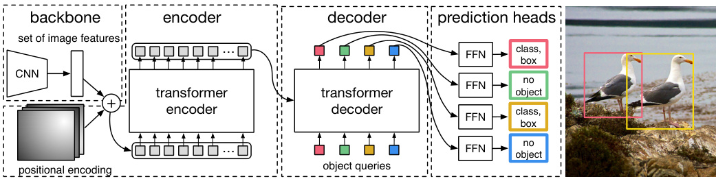
Fig. 2: DETR uses a conventional CNN backbone to learn a 2D representation of an input image. The model flattens it and supplements it with a positional encoding before passing it into a transformer encoder. A transformer decoder then takes as input a small fixed number of learned positional embeddings, which we call object queries, and additionally attends to the encoder output. We pass each output embedding of the decoder to a shared feed forward network (FFN) that predicts either a detection (class and bounding box) or a “no object” class.
图 2: DETR采用传统CNN主干网络学习输入图像的二维表征。模型将其展平并添加位置编码后输入Transformer编码器。随后,Transformer解码器以少量固定数量的可学习位置嵌入(称为对象查询)作为输入,同时关注编码器输出。我们将解码器的每个输出嵌入传递给共享前馈网络(FFN),该网络预测检测结果(类别和边界框)或"无对象"类别。
Transformer decoder. The decoder follows the standard architecture of the transformer, transforming $N$ embeddings of size $d$ using multi-headed self- and encoder-decoder attention mechanisms. The difference with the original transformer is that our model decodes the $N$ objects in parallel at each decoder layer, while Vaswani et al. [47] use an auto regressive model that predicts the output sequence one element at a time. We refer the reader unfamiliar with the concepts to the supplementary material. Since the decoder is also permutation-invariant, the $N$ input embeddings must be different to produce different results. These input embeddings are learnt positional encodings that we refer to as object queries, and similarly to the encoder, we add them to the input of each attention layer. The $N$ object queries are transformed into an output embedding by the decoder. They are then independently decoded into box coordinates and class labels by a feed forward network (described in the next subsection), resulting $N$ final predictions. Using self- and encoder-decoder attention over these embeddings, the model globally reasons about all objects together using pair-wise relations between them, while being able to use the whole image as context.
Transformer解码器。该解码器遵循Transformer的标准架构,通过多头自注意力和编码器-解码器注意力机制对尺寸为$d$的$N$个嵌入进行转换。与原始Transformer的不同之处在于,我们的模型在每一解码层并行解码$N$个对象,而Vaswani等人[47]采用自回归模型逐元素预测输出序列。不熟悉相关概念的读者可参阅补充材料。由于解码器同样具有排列不变性,$N$个输入嵌入必须各不相同才能产生不同结果。这些输入嵌入是学习得到的位置编码,我们称之为对象查询(object queries),与编码器类似,我们将其添加到每个注意力层的输入中。解码器将这$N$个对象查询转换为输出嵌入,随后通过前馈网络(详见下节)独立解码为边界框坐标和类别标签,最终得到$N$个预测结果。通过对这些嵌入应用自注意力和编码器-解码器注意力,模型能基于对象间的成对关系全局推理所有对象,同时将整幅图像作为上下文信息加以利用。
Prediction feed-forward networks (FFNs). The final prediction is computed by a 3-layer perceptron with ReLU activation function and hidden dimension $d$ , and a linear projection layer. The FFN predicts the normalized center coordinates, height and width of the box w.r.t. the input image, and the linear layer predicts the class label using a softmax function. Since we predict a fixed-size set of $N$ bounding boxes, where $N$ is usually much larger than the actual number of objects of interest in an image, an additional special class label $\scriptscriptstyle\mathcal{L}$ is used to represent that no object is detected within a slot. This class plays a similar role to the “background” class in the standard object detection approaches.
预测前馈网络 (FFNs)。最终预测由一个3层感知机计算得出,该感知机使用ReLU激活函数和隐藏维度$d$,以及一个线性投影层。FFN预测相对于输入图像的归一化边界框中心坐标、高度和宽度,线性层则通过softmax函数预测类别标签。由于我们预测的是固定数量$N$个边界框,而$N$通常远大于图像中实际感兴趣对象的数量,因此额外引入一个特殊类别标签$\scriptscriptstyle\mathcal{L}$来表示该槽位未检测到任何对象。该类别在标准目标检测方法中起到与"背景"类别类似的作用。
Auxiliary decoding losses. We found helpful to use auxiliary losses [1] in decoder during training, especially to help the model output the correct number of objects of each class. We add prediction FFNs and Hungarian loss after each decoder layer. All predictions FFNs share their parameters. We use an additional shared layer-norm to normalize the input to the prediction FFNs from different decoder layers.
辅助解码损失。我们发现,在训练过程中于解码器中使用辅助损失 [1] 很有帮助,尤其是能协助模型输出每个类别的正确对象数量。我们在每个解码器层后添加预测 FFN (Feed-Forward Network) 和匈牙利损失。所有预测 FFN 共享参数,并通过额外的共享层归一化 (layer-norm) 对不同解码器层输入预测 FFN 的数据进行标准化处理。
4 Experiments
4 实验
We show that DETR achieves competitive results compared to Faster R-CNN in quantitative evaluation on COCO. Then, we provide a detailed ablation study of the architecture and loss, with insights and qualitative results. Finally, to show that DETR is a versatile and extensible model, we present results on panoptic segmentation, training only a small extension on a fixed DETR model. We provide code and pretrained models to reproduce our experiments at https://github.com/facebook research/detr.
我们证明DETR在COCO定量评估中与Faster R-CNN相比具有竞争力。接着,我们对架构和损失函数进行了详细的消融研究,并提供了见解和定性结果。最后,为了展示DETR是一个多功能且可扩展的模型,我们给出了全景分割的结果,仅需在固定DETR模型上训练一个小型扩展。我们在https://github.com/facebookresearch/detr提供了代码和预训练模型以复现实验。
Dataset. We perform experiments on COCO 2017 detection and panoptic segmentation datasets [24,18], containing 118k training images and 5k validation images. Each image is annotated with bounding boxes and panoptic segmentation. There are 7 instances per image on average, up to 63 instances in a single image in training set, ranging from small to large on the same images. If not specified, we report AP as bbox AP, the integral metric over multiple thresholds. For comparison with Faster R-CNN we report validation AP at the last training epoch, for ablations we report median over validation results from the last 10 epochs.
数据集。我们在COCO 2017检测与全景分割数据集[24,18]上进行实验,该数据集包含11.8万张训练图像和5000张验证图像。每张图像均标注有边界框和全景分割信息。训练集中平均每张图像包含7个实例,单张图像最多含63个实例,且同一图像中的实例尺寸从小型到大型不等。若无特别说明,我们采用边界框平均精度(bbox AP)作为评估指标,即多阈值下的综合度量指标。与Faster R-CNN对比时报告最终训练周期的验证集AP值,消融实验则取最后10个训练周期验证结果的中位数。
Technical details. We train DETR with AdamW [26] setting the initial transformer’s learning rate to $10^{-4}$ , the backbone’s to $10^{-5}$ , and weight decay to $10^{-4}$ . All transformer weights are initialized with Xavier init [11], and the backbone is with ImageNet-pretrained ResNet model [15] from torch vision with frozen batchnorm layers. We report results with two different backbones: a ResNet50 and a ResNet-101. The corresponding models are called respectively DETR and DETR-R101. Following [21], we also increase the feature resolution by adding a dilation to the last stage of the backbone and removing a stride from the first convolution of this stage. The corresponding models are called respectively DETR-DC5 and DETR-DC5-R101 (dilated C5 stage). This modification increases the resolution by a factor of two, thus improving performance for small objects, at the cost of a 16x higher cost in the self-attentions of the encoder, leading to an overall 2x increase in computational cost. A full comparison of FLOPs of these models and Faster R-CNN is given in Table 1.
技术细节。我们使用AdamW [26]训练DETR,将初始Transformer的学习率设为$10^{-4}$,主干网络设为$10^{-5}$,权重衰减设为$10^{-4}$。所有Transformer权重采用Xavier初始化[11],主干网络采用torch vision提供的ImageNet预训练ResNet模型[15]并冻结批归一化层。我们报告了两种不同主干网络的结果:ResNet50和ResNet-101,对应模型分别称为DETR和DETR-R101。参照[21]的方法,我们通过在主干的最后阶段添加膨胀卷积并移除该阶段第一个卷积的步长来提升特征分辨率,对应模型分别称为DETR-DC5和DETR-DC5-R101(膨胀C5阶段)。这一修改将分辨率提高两倍,从而改善小物体检测性能,但会导致编码器自注意力计算成本增加16倍,总体计算量增加2倍。这些模型与Faster R-CNN的FLOPs完整对比见 表1。
We use scale augmentation, resizing the input images such that the shortest side is at least 480 and at most 800 pixels while the longest at most 1333 [50]. To help learning global relationships through the self-attention of the encoder, we also apply random crop augmentations during training, improving the performance by approximately 1 AP. Specifically, a train image is cropped with probability 0.5 to a random rectangular patch which is then resized again to 800-1333. The transformer is trained with default dropout of 0.1. At inference
我们采用尺度增强策略,将输入图像的最短边调整至至少480像素、至多800像素,同时最长边不超过1333像素[50]。为通过编码器的自注意力机制帮助学习全局关系,训练过程中还应用了随机裁剪增强,使性能提升约1 AP。具体而言,训练图像有50%概率被随机裁剪为矩形区域,随后再次调整至800-1333像素范围。Transformer模型训练时采用默认0.1的dropout率。推理阶段...
Table 1: Comparison with Faster R-CNN with a ResNet-50 and ResNet-101 backbones on the COCO validation set. The top section shows results for Faster R-CNN models in Detectron2 [50], the middle section shows results for Faster R-CNN models with GIoU [38], random crops train-time augmentation, and the long 9x training schedule. DETR models achieve comparable results to heavily tuned Faster R-CNN baselines, having lower APS but greatly improved AP $\llcorner$ . We use torch script Faster R-CNN and DETR models to measure FLOPS and FPS. Results without R101 in the name correspond to ResNet-50.
表 1: 基于ResNet-50和ResNet-101骨干网络的Faster R-CNN在COCO验证集上的性能对比。顶部区域显示Detectron2 [50]中Faster R-CNN模型的测试结果,中部区域展示采用GIoU [38]、随机裁剪训练时数据增强及9x长训练周期的Faster R-CNN模型结果。DETR模型与经过深度调优的Faster R-CNN基线表现相当,APS略低但AP$\llcorner$显著提升。我们使用torch script版本的Faster R-CNN和DETR模型测量FLOPS与FPS。未标注R101的名称对应ResNet-50架构。
| Model | GFLOPS/FPS#params | AP AP50 AP75 APs APM APL |
| Faster RCNN-DC5 39.0 | 320/16 166M | |
| Faster RCNN-FPN | 60.5 180/26 42M 40.2 61.0 | |
| Faster RCNN-R101-FPN 246/20 | 43.8 24.2 43.5 52.0 60M 42.0 62.5 45.9 25.2 45.6 54.6 | |
| 166M 41.1 61.4 44.3 22.9 | ||
| Faster RCNN-DC5+ 320/16 Faster RCNN-FPN+ 180/26 | 45.9 55.0 42M 42.0 62.1 45.5 26.6 45.4 53.4 | |
| Faster RCNN-R101-FPN+ 246/20 | 60M 44.0 63.9 47.8 27.2 | |
| 56.0 41M 42.0 62.4 44.2 20.5 45.8 | ||
| DETR 86/28 DETR-DC5 | 61.1 41M 43.3 63.1 45.9 22.5 47.3 61.1 | |
| 187/12 DETR-R101 152/20 | 60M 43.5 63.8 46.4 21.9 48.0 |
| 模型 | GFLOPS/FPS#参数 | AP AP50 AP75 APs APM APL |
|---|---|---|
| Faster RCNN-DC5 39.0 | 320/16 166M | - |
| Faster RCNN-FPN | 60.5 180/26 42M 40.2 61.0 | - |
| Faster RCNN-R101-FPN 246/20 | 43.8 24.2 43.5 52.0 60M 42.0 62.5 45.9 25.2 45.6 54.6 | - |
| 166M 41.1 61.4 44.3 22.9 | - | |
| Faster RCNN-DC5+ 320/16 Faster RCNN-FPN+ 180/26 | 45.9 55.0 42M 42.0 62.1 45.5 26.6 45.4 53.4 | - |
| Faster RCNN-R101-FPN+ 246/20 | 60M 44.0 63.9 47.8 27.2 | - |
| 56.0 41M 42.0 62.4 44.2 20.5 45.8 | - | |
| DETR 86/28 DETR-DC5 | 61.1 41M 43.3 63.1 45.9 22.5 47.3 61.1 | - |
| DETR-R101 152/20 | 60M 43.5 63.8 46.4 21.9 48.0 | - |
time, some slots predict empty class. To optimize for AP, we override the prediction of these slots with the second highest scoring class, using the corresponding confidence. This improves AP by 2 points compared to filtering out empty slots. Other training hyper parameters can be found in section A.4. For our ablation experiments we use training schedule of 300 epochs with a learning rate drop by a factor of 10 after 200 epochs, where a single epoch is a pass over all training images once. Training the baseline model for 300 epochs on 16 V100 GPUs takes 3 days, with 4 images per GPU (hence a total batch size of 64). For the longer schedule used to compare with Faster R-CNN we train for 500 epochs with learning rate drop after 400 epochs. This schedule adds 1.5 AP compared to the shorter schedule.
训练过程中,部分预测框会输出空类别。为优化平均精度(AP),我们改用置信度第二高的类别覆盖这些空类别预测。相比直接过滤空类别框,该方法可提升2个AP点。其余训练超参数详见附录A.4。消融实验采用300轮训练方案:前200轮学习率不变,之后降至1/10(每轮完整遍历训练集一次)。基线模型在16块V100 GPU(每卡4张图像,总批次大小64)训练300轮需3天。与Faster R-CNN对比时采用500轮长周期方案(400轮后降学习率),该方案较300轮周期可提升1.5 AP。
4.1 Comparison with Faster R-CNN
4.1 与Faster R-CNN的对比
Transformers are typically trained with Adam or Adagrad optimizers with very long training schedules and dropout, and this is true for DETR as well. Faster R-CNN, however, is trained with SGD with minimal data augmentation and we are not aware of successful applications of Adam or dropout. Despite these differences we attempt to make a Faster R-CNN baseline stronger. To align it with DETR, we add generalized IoU [38] to the box loss, the same random crop augmentation and long training known to improve results [13]. Results are presented in Table 1. In the top section we show Faster R-CNN results from Detectron2 Model Zoo [50] for models trained with the 3x schedule. In the middle section we show results (with a “+”) for the same models but trained with the 9x schedule (109 epochs) and the described enhancements, which in total adds 1-2 AP. In the last section of Table 1 we show the results for multiple DETR models. To be comparable in the number of parameters we choose a model with 6 transformer and 6 decoder layers of width 256 with 8 attention heads. Like Faster R-CNN with FPN this model has 41.3M parameters, out of which 23.5M are in ResNet-50, and 17.8M are in the transformer. Even though both Faster R-CNN and DETR are still likely to further improve with longer training, we can conclude that DETR can be competitive with Faster R-CNN with the same number of parameters, achieving 42 AP on the COCO val subset. The way DETR achieves this is by improving AP $\perp$ (+7.8), however note that the model is still lagging behind in APS (-5.5). DETR-DC5 with the same number of parameters and similar FLOP count has higher AP, but is still significantly behind in APS too. Faster R-CNN and DETR with ResNet-101 backbone show comparable results as well.
Transformer通常使用Adam或Adagrad优化器进行长时间训练并配合dropout,DETR也是如此。而Faster R-CNN则使用SGD进行训练,数据增强较少,且我们尚未发现Adam或dropout在其上的成功应用。尽管存在这些差异,我们仍尝试提升Faster R-CNN的基线性能。为了与DETR对齐,我们在边界框损失函数中加入了广义IoU [38]、相同的随机裁剪增强策略以及已知能提升效果的长时训练方案 [13]。结果如表1所示。
表1顶部展示了Detectron2模型库 [50] 中采用3倍训练周期的Faster R-CNN结果。中间部分(标注"+")展示相同模型采用9倍训练周期(109轮次)及前述增强策略后的结果,总体带来1-2 AP提升。表1最后部分展示了多个DETR模型的结果。为保持参数量可比性,我们选择具有6层宽度为256的Transformer编码器和解码器(8个注意力头)的模型。与带FPN的Faster R-CNN类似,该模型具有4130万参数(ResNet-50占2350万,Transformer占1780万)。尽管Faster R-CNN和DETR都可能通过更长时间训练继续提升,但可以得出结论:在参数量相同的情况下,DETR在COCO验证集上达到42 AP,已具备与Faster R-CNN竞争的实力。DETR主要通过提升AP$\perp$(+7.8)实现这一目标,但需注意该模型在APS(-5.5)方面仍存在差距。具有相同参数量和类似FLOPs的DETR-DC5虽然AP更高,但在APS方面同样显著落后。采用ResNet-101骨干网络时,Faster R-CNN与DETR也表现出可比的结果。
Table 2: Effect of encoder size. Each row corresponds to a model with varied number of encoder layers and fixed number of decoder layers. Performance gradually improves with more encoder layers.
| #layers | GFLOPS/FPS | #params | AP | AP50 | APs | APM | APL |
| 0 | 76/28 | 33.4M | 36.7 | 57.4 | 16.8 | 39.6 | 54.2 |
| 3 | 81/25 | 37.4M | 40.1 | 60.6 | 18.5 | 43.8 | 58.6 |
| 6 | 86/23 | 41.3M | 40.6 | 61.6 | 19.9 | 44.3 | 60.2 |
| 12 | 95/20 | 49.2M | 41.6 | 62.1 | 19.8 | 44.9 | 61.9 |
表 2: 编码器大小的影响。每行对应一个编码器层数不同但解码器层数固定的模型。随着编码器层数增加,性能逐渐提升。
| #layers | GFLOPS/FPS | #params | AP | AP50 | APs | APM | APL |
|---|---|---|---|---|---|---|---|
| 0 | 76/28 | 33.4M | 36.7 | 57.4 | 16.8 | 39.6 | 54.2 |
| 3 | 81/25 | 37.4M | 40.1 | 60.6 | 18.5 | 43.8 | 58.6 |
| 6 | 86/23 | 41.3M | 40.6 | 61.6 | 19.9 | 44.3 | 60.2 |
| 12 | 95/20 | 49.2M | 41.6 | 62.1 | 19.8 | 44.9 | 61.9 |
4.2 Ablations
4.2 消融实验
Attention mechanisms in the transformer decoder are the key components which model relations between feature representations of different detections. In our ablation analysis, we explore how other components of our architecture and loss influence the final performance. For the study we choose ResNet-50-based DETR model with 6 encoder, 6 decoder layers and width 256. The model has 41.3M parameters, achieves 40.6 and 42.0 AP on short and long schedules respectively, and runs at 28 FPS, similarly to Faster R-CNN-FPN with the same backbone.
Transformer解码器中的注意力机制是建模不同检测特征表示之间关系的关键组件。在我们的消融分析中,我们探讨了架构和损失函数的其他组件如何影响最终性能。为此研究,我们选择了基于ResNet-50的DETR模型,该模型具有6个编码器层、6个解码器层和256的宽度。该模型拥有41.3M参数,在短训练计划和长训练计划下分别达到40.6和42.0 AP,并以28 FPS的速度运行,与具有相同骨干网络的Faster R-CNN-FPN相当。
Number of encoder layers. We evaluate the importance of global imagelevel self-attention by changing the number of encoder layers (Table 2). Without encoder layers, overall AP drops by 3.9 points, with a more significant drop of 6.0 AP on large objects. We hypothesize that, by using global scene reasoning, the encoder is important for disentangling objects. In Figure 3, we visualize the attention maps of the last encoder layer of a trained model, focusing on a few points in the image. The encoder seems to separate instances already, which likely simplifies object extraction and localization for the decoder.
编码器层数。我们通过改变编码器层数来评估全局图像级自注意力机制的重要性(表2)。当没有编码器层时,整体AP(平均精度)下降了3.9点,其中大物体的AP下降更为显著,达到6.0。我们假设,通过利用全局场景推理,编码器对于分离物体至关重要。在图3中,我们可视化了一个训练好的模型最后一层编码器的注意力图,重点关注图像中的几个点。编码器似乎已经能够分离实例,这可能简化了解码器的物体提取和定位过程。
Number of decoder layers. We apply auxiliary losses after each decoding layer (see Section 3.2), hence, the prediction FFNs are trained by design to predict objects out of the outputs of every decoder layer. We analyze the importance of each decoder layer by evaluating the objects that would be predicted at each stage of the decoding (Fig. 4). Both AP and AP $^{50}$ improve after every layer, totalling into a very significant +8.2/9.5 AP improvement between the first and the last layer. With its set-based loss, DETR does not need NMS by design. To verify this we run a standard NMS procedure with default parameters [50] for the outputs after each decoder. NMS improves performance for the predictions from the first decoder. This can be explained by the fact that a single decoding layer of the transformer is not able to compute any cross-correlations between the output elements, and thus it is prone to making multiple predictions for the same object. In the second and subsequent layers, the self-attention mechanism over the activation s allows the model to inhibit duplicate predictions. We observe that the improvement brought by NMS diminishes as depth increases. At the last layers, we observe a small loss in AP as NMS incorrectly removes true positive predictions.
解码器层数。我们在每个解码层后应用辅助损失(见第3.2节),因此预测FFN(前馈网络)在设计上就被训练为从每个解码层的输出中预测目标。通过评估解码各阶段预测的目标(图4),我们分析了每个解码层的重要性。AP和AP$^{50}$在每一层后都有提升,首层与末层之间总计实现了+8.2/9.5 AP的显著提升。基于集合损失的设计使DETR无需NMS(非极大值抑制)。为验证这一点,我们对每个解码器输出使用默认参数[50]运行标准NMS流程。NMS提升了首层解码器的预测性能,这是因为Transformer单层解码器无法计算输出元素间的互相关性,容易对同一目标产生多次预测。在第二层及后续层中,基于激活值的自注意力机制使模型能够抑制重复预测。随着深度增加,NMS带来的改进逐渐减弱。在最后几层中,由于NMS错误移除真实正例预测,我们观察到AP出现小幅下降。
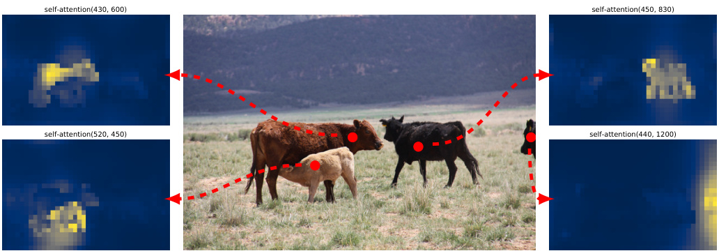
Fig. 3: Encoder self-attention for a set of reference points. The encoder is able to separate individual instances. Predictions are made with baseline DETR model on a validation set image.
图 3: 参考点集合的编码器自注意力机制。编码器能够区分不同实例。预测结果由基线DETR模型在验证集图像上生成。
Similarly to visualizing encoder attention, we visualize decoder attentions in Fig. 6, coloring attention maps for each predicted object in different colors. We observe that decoder attention is fairly local, meaning that it mostly attends to object extremities such as heads or legs. We hypothesis e that after the encoder has separated instances via global attention, the decoder only needs to attend to the extremities to extract the class and object boundaries.
与可视化编码器注意力类似,我们在图6中可视化解码器注意力,用不同颜色标注每个预测对象的注意力图。我们观察到解码器注意力具有明显的局部性,主要关注对象的末端部位(如头部或腿部)。我们假设在编码器通过全局注意力分离实例后,解码器只需关注这些末端部位即可提取类别和对象边界。
Importance of FFN. FFN inside tr an former s can be seen as $1\times1$ convolutional layers, making encoder similar to attention augmented convolutional networks [3]. We attempt to remove it completely leaving only attention in the transformer layers. By reducing the number of network parameters from 41.3M to 28.7M, leaving only 10.8M in the transformer, performance drops by 2.3 AP, we thus conclude that FFN are important for achieving good results.
FFN的重要性。Transformer中的FFN可被视为$1\times1$卷积层,这使得编码器类似于注意力增强卷积网络[3]。我们尝试完全移除它,仅在Transformer层中保留注意力机制。通过将网络参数量从41.3M减少到28.7M(Transformer中仅剩10.8M),性能下降了2.3 AP,因此我们得出结论:FFN对获得良好结果至关重要。
Importance of positional encodings. There are two kinds of positional encodings in our model: spatial positional encodings and output positional encodings (object queries). We experiment with various combinations of fixed and learned encodings, results can be found in table 3. Output positional encodings are required and cannot be removed, so we experiment with either passing them once at decoder input or adding to queries at every decoder attention layer. In the first experiment we completely remove spatial positional encodings and pass output positional encodings at input and, interestingly, the model still achieves more than 32 AP, losing 7.8 AP to the baseline. Then, we pass fixed sine spatial positional encodings and the output encodings at input once, as in the original transformer [47], and find that this leads to 1.4 AP drop compared to passing the positional encodings directly in attention. Learned spatial encodings passed to the attentions give similar results. Surprisingly, we find that not passing any spatial encodings in the encoder only leads to a minor AP drop of 1.3 AP. When we pass the encodings to the attentions, they are shared across all layers, and the output encodings (object queries) are always learned.
位置编码的重要性。我们的模型中有两种位置编码:空间位置编码和输出位置编码(object queries)。我们尝试了固定编码和学习编码的各种组合,结果见表3。输出位置编码是必需的且无法移除,因此我们尝试在解码器输入端传递一次或在每个解码器注意力层添加到查询中。在第一个实验中,我们完全移除了空间位置编码,仅在输入端传递输出位置编码,有趣的是,模型仍能达到超过32 AP的成绩,比基线下降了7.8 AP。接着,我们像原始Transformer [47]那样,在输入端传递固定的正弦空间位置编码和输出编码一次,发现这比直接在注意力中传递位置编码导致AP下降了1.4。传递给注意力的学习空间编码结果类似。令人惊讶的是,我们发现不在编码器中传递任何空间编码仅导致AP轻微下降1.3。当我们将编码传递给注意力时,它们在所有层之间共享,而输出编码(object queries)始终是学习的。
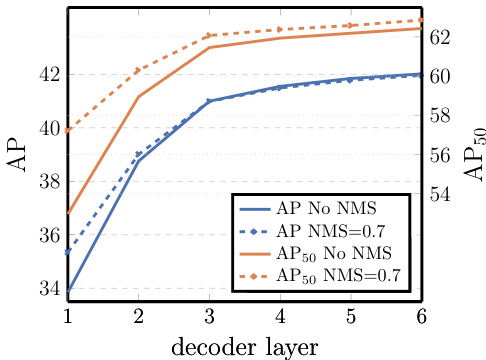
Fig. 4: AP and AP50 performance after each decoder layer. A single long schedule baseline model is evaluated. DETR does not need NMS by design, which is validated by this figure. NMS lowers AP in the final layers, removing TP predictions, but improves AP in the first decoder layers, removing double predictions, as there is no communication in the first layer, and slightly improves AP50.
图 4: 各解码器层后的 AP (Average Precision) 和 AP50 性能表现。评估对象为单一长周期基线模型。DETR 在设计上无需 NMS (Non-Maximum Suppression),该图验证了这一点。NMS 在最后几层会降低 AP 值(因移除了正确预测),但在初始解码层能提升 AP(消除了重复预测),这是由于首层缺乏信息交互所致,同时 AP50 略有提升。
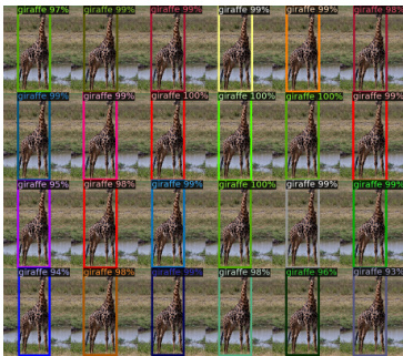
Fig. 5: Out of distribution genera liz ation for rare classes. Even though no image in the training set has more than 13 giraffes, DETR has no difficulty generalizing to 24 and more instances of the same class.
图 5: 稀有类别在分布外场景的泛化能力。尽管训练集中没有任何图像包含超过13只长颈鹿,DETR仍能轻松泛化至24只甚至更多同类实例。
Given these ablations, we conclude that transformer components: the global self-attention in encoder, FFN, multiple decoder layers, and positional encodings, all significantly contribute to the final object detection performance.
根据这些消融实验,我们得出结论:Transformer组件(编码器中的全局自注意力机制、FFN、多层解码器以及位置编码)都对最终的目标检测性能有显著贡献。
Loss ablations. To evaluate the importance of different components of the matching cost and the loss, we train several models turning them on and off. There are three components to the loss: classification loss, $\ell_{1}$ bounding box distance loss, and GIoU [38] loss. The classification loss is essential for training and cannot be turned off, so we train a model without bounding box distance loss, and a model without the GIoU loss, and compare with baseline, trained with all three losses. Results are presented in table 4. GIoU loss on its own accounts for most of the model performance, losing only 0.7 AP to the baseline with combined losses. Using $\ell_{1}$ without GIoU shows poor results. We only studied simple ablations of different losses (using the same weighting every time), but other means of combining them may achieve different results.
损失消融实验。为评估匹配成本和损失函数中不同组件的重要性,我们通过开关组件的方式训练了多个模型。损失函数包含三个组成部分:分类损失、$\ell_{1}$边界框距离损失和GIoU[38]损失。分类损失对训练至关重要且不可关闭,因此我们分别训练了不含边界框距离损失的模型、不含GIoU损失的模型,并与同时使用三种损失的基线模型进行对比。结果如表4所示:单独使用GIoU损失即可实现模型大部分性能,仅比组合损失的基线低0.7 AP;单独使用$\ell_{1}$而不结合GIoU的效果较差。我们仅对不同损失进行了简单消融研究(每次使用相同权重),其他组合方式可能会产生不同结果。
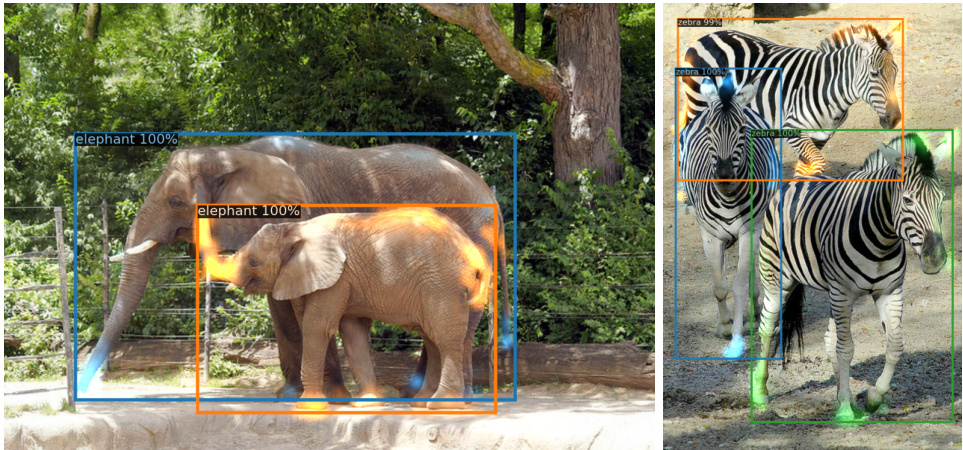
Fig. 6: Visualizing decoder attention for every predicted object (images from COCO val set). Predictions are made with DETR-DC5 model. Attention scores are coded with different colors for different objects. Decoder typically attends to object extremities, such as legs and heads. Best viewed in color.
图 6: 可视化每个预测物体的解码器注意力(图像来自COCO验证集)。预测使用DETR-DC5模型完成。不同物体的注意力分数用不同颜色编码。解码器通常会关注物体 extremities (肢体末端),例如腿部和头部。建议彩色查看。
Table 3: Results for different positional encodings compared to the baseline (last row), which has fixed sine pos. encodings passed at every attention layer in both the encoder and the decoder. Learned embeddings are shared between all layers. Not using spatial positional encodings leads to a significant drop in AP. Interestingly, passing them in decoder only leads to a minor AP drop. All these models use learned output positional encodings.
| spatial pos. enc. | outputpos.enc. decoder | |||||
| encoder | decoder | △ | AP50 | △ | ||
| none | none | learnedatinput | 32.8 | -7.8 | 55.2 | -6.5 |
| sine atinput | sine atinput | learnedatinput | 39.2 | -1.4 | 60.0 | -1.6 |
| learnedat attn. | learnedatattn. | learnedatattn. | 39.6 | -1.0 | 60.7 | -0.9 |
| none | sineatattn. | learnedatattn. | 39.3 | -1.3 | 60.3 | -1.4 |
| sineatattn. | sineatattn. | learnedatattn. | 40.6 | 61.6 | ||
表 3: 不同位置编码与基线(最后一行)的对比结果。基线在编码器和解码器的每个注意力层都使用固定的正弦位置编码。学习到的嵌入在所有层之间共享。不使用空间位置编码会导致AP显著下降。有趣的是,仅在解码器中传递它们会导致AP轻微下降。所有这些模型都使用学习到的输出位置编码。
| 空间位置编码 | 输出位置编码解码器 | △ | AP50 | △ |
|---|---|---|---|---|
| 无 | 无 | 输入学习 | 32.8 | -7.8 |
| 输入正弦 | 输入正弦 | 输入学习 | 39.2 | -1.4 |
| 注意力学习 | 注意力学习 | 注意力学习 | 39.6 | -1.0 |
| 无 | 注意力正弦 | 注意力学习 | 39.3 | -1.3 |
| 注意力正弦 | 注意力正弦 | 注意力学习 | 40.6 |
Table 4: Effect of loss components on AP. We train two models turning off $\ell_{1}$ loss, and GIoU loss, and observe that $\ell_{1}$ gives poor results on its own, but when combined with GIoU improves $\mathrm{AP_{M}}$ and $\mathrm{AP_{L}}$ . Our baseline (last row) combines both losses.
| class | l1 | GIoU | AP | △ | AP50 | △ | APs | APM | APL |
| 人 | 人 | 35.8 | -4.8 | 57.3 | -4.4 | 13.7 | 39.8 | 57.9 | |
| 人 | √ | 39.9 | -0.7 | 61.6 | 0 | 19.9 | 43.2 | 57.9 | |
| √ | 人 | √ | 40.6 | 61.6 | 19.9 | 44.3 | 60.2 |
表 4: 损失分量对AP的影响。我们训练了两个模型,分别关闭$\ell_{1}$损失和GIoU损失,观察到$\ell_{1}$单独使用时效果较差,但与GIoU结合后能提升$\mathrm{AP_{M}}$和$\mathrm{AP_{L}}$。我们的基线方案(最后一行)结合了两种损失。
| class | l1 | GIoU | AP | △ | AP50 | △ | APs | APM | APL |
|---|---|---|---|---|---|---|---|---|---|
| 人 | 人 | 35.8 | -4.8 | 57.3 | -4.4 | 13.7 | 39.8 | 57.9 | |
| 人 | √ | 39.9 | -0.7 | 61.6 | 0 | 19.9 | 43.2 | 57.9 | |
| √ | 人 | √ | 40.6 | 61.6 | 19.9 | 44.3 | 60.2 |

Fig. 7: Visualization of all box predictions on all images from COCO 2017 val set for 20 out of total $N=100$ prediction slots in DETR decoder. Each box prediction is represented as a point with the coordinates of its center in the 1-by-1 square normalized by each image size. The points are color-coded so that green color corresponds to small boxes, red to large horizontal boxes and blue to large vertical boxes. We observe that each slot learns to specialize on certain areas and box sizes with several operating modes. We note that almost all slots have a mode of predicting large image-wide boxes that are common in COCO dataset.
图 7: DETR解码器中20个预测槽(共$N=100$个)在COCO 2017验证集所有图像上的边界框预测可视化。每个边界框预测表示为一个点,其中心坐标经图像尺寸归一化至1×1方格内。颜色编码规则为:绿色对应小框,红色对应大横框,蓝色对应大竖框。我们观察到每个槽会学习专注于特定区域和框尺寸,并呈现多种工作模式。值得注意的是,几乎所有槽都具有预测图像范围大框的模式(这在COCO数据集中很常见)。
4.3 Analysis
4.3 分析
Decoder output slot analysis In Fig. 7 we visualize the boxes predicted by different slots for all images in COCO 2017 val set. DETR learns different specialization for each query slot. We observe that each slot has several modes of operation focusing on different areas and box sizes. In particular, all slots have the mode for predicting image-wide boxes (visible as the red dots aligned in the middle of the plot). We hypothesize that this is related to the distribution of objects in COCO.
解码器输出槽分析
在图7中,我们可视化了COCO 2017验证集所有图像中不同槽预测的边界框。DETR为每个查询槽学习了不同的专长。我们观察到,每个槽具有多种操作模式,分别关注不同区域和框尺寸。值得注意的是,所有槽都具备预测全图范围边界框的模式(图中显示为中间对齐的红点)。我们推测这与COCO数据集中物体的分布特性有关。
Generalization to unseen numbers of instances. Some classes in COCO are not well represented with many instances of the same class in the same image. For example, there is no image with more than 13 giraffes in the training set. We create a synthetic image $^{3}$ to verify the generalization ability of DETR (see Figure 5). Our model is able to find all 24 giraffes on the image which is clearly out of distribution. This experiment confirms that there is no strong class-specialization in each object query.
泛化到未见过的实例数量。COCO数据集中某些类别的图像在同一张图片中缺乏大量同类实例的充分表征。例如,训练集中没有包含超过13只长颈鹿的图片。我们创建了一张合成图像$^{3}$来验证DETR的泛化能力(参见图5)。我们的模型能够成功检测出图中明显超出分布范围的24只长颈鹿。该实验证实了每个对象查询(object query)不存在强烈的类别专一性。
4.4 DETR for panoptic segmentation
4.4 用于全景分割的DETR
Panoptic segmentation [19] has recently attracted a lot of attention from the computer vision community. Similarly to the extension of Faster R-CNN [37] to Mask R-CNN [14], DETR can be naturally extended by adding a mask head on top of the decoder outputs. In this section we demonstrate that such a head can be used to produce panoptic segmentation [19] by treating stuff and thing classes in a unified way. We perform our experiments on the panoptic annotations of the COCO dataset that has 53 stuff categories in addition to 80 things categories.
全景分割 [19] 最近引起了计算机视觉领域的广泛关注。与 Faster R-CNN [37] 扩展到 Mask R-CNN [14] 类似,DETR 只需在解码器输出端添加掩码头就能自然扩展。本节我们将证明,通过统一处理背景(stuff)和物体(thing)类别,该头部可用于生成全景分割 [19]。我们在 COCO 数据集的全景标注上进行了实验,该数据集除80个物体类别外还包含53个背景类别。

Fig. 8: Illustration of the panoptic head. A binary mask is generated in parallel for each detected object, then the masks are merged using pixel-wise argmax.
图 8: 全景分割头结构示意图。每个检测到的对象会并行生成一个二值掩码,随后通过逐像素 argmax 操作合并这些掩码。

Fig. 9: Qualitative results for panoptic segmentation generated by DETR-R101. DETR produces aligned mask predictions in a unified manner for things and stuff.
图 9: DETR-R101 生成的全景分割定性结果。DETR 以统一方式为物体 (things) 和背景 (stuff) 生成对齐的掩码预测。
We train DETR to predict boxes around both stuff and things classes on COCO, using the same recipe. Predicting boxes is required for the training to be possible, since the Hungarian matching is computed using distances between boxes. We also add a mask head which predicts a binary mask for each of the predicted boxes, see Figure 8. It takes as input the output of transformer decoder for each object and computes multi-head (with $M$ heads) attention scores of this embedding over the output of the encoder, generating $M$ attention heatmaps per object in a small resolution. To make the final prediction and increase the resolution, an FPN-like architecture is used. We describe the architecture in more details in the supplement. The final resolution of the masks has stride 4 and each mask is supervised independently using the DICE/F-1 loss [28] and Focal loss [23].
我们采用相同方案训练DETR在COCO数据集上预测物体(stuff)和实体(things)类别的边界框。由于匈牙利匹配是通过计算框间距离实现的,预测边界框是训练的必要条件。我们还添加了一个掩码头(mask head),用于为每个预测框生成二值掩码(见图8)。该模块以每个对象经过transformer解码器的输出作为输入,通过计算该嵌入向量与编码器输出的多头注意力分数(共$M$个头),为每个对象生成$M$张低分辨率注意力热图。为生成最终预测并提高分辨率,采用了类FPN架构。补充材料中提供了更详细的架构说明。最终掩码的分辨率步长为4,每个掩码使用DICE/F-1损失[28]和Focal损失[23]进行独立监督。
The mask head can be trained either jointly, or in a two steps process, where we train DETR for boxes only, then freeze all the weights and train only the mask head for 25 epochs. Experimentally, these two approaches give similar results, we report results using the latter method since it results in a shorter total wall-clock time training.
掩码头部可以采用联合训练方式,也可分两步进行:先仅训练DETR的边界框检测部分,随后冻结所有权重并单独训练掩码头部25个周期。实验表明这两种方法效果相近,我们采用后者汇报结果,因其总训练时长更短。
Table 5: Comparison with the state-of-the-art methods UPSNet [51] and Panoptic FPN [18] on the COCO val dataset We retrained Pan optic FP N with the same dataaugmentation as DETR, on a 18x schedule for fair comparison. UPSNet uses the 1x schedule, UPSNet-M is the version with multiscale test-time augmentations.
| Model | Backbone | PQ | SQ | RQ | PQth | SQth | RQ th | PQ )st | SQst | RQst | AP |
| PanopticFPN++ | R50 | 42.4 | 79.3 | 51.6 | 49.2 | 82.4 | 58.8 | 32.3 | 74.8 | 40.6 | 37.7 |
| UPSnet | R50 | 42.5 | 78.0 | 52.5 | 48.6 | 79.4 | 59.6 | 33.4 | 75.9 | 41.7 | 34.3 |
| UPSnet-M | R50 | 43.0 | 79.1 | 52.8 | 48.9 | 79.7 | 59.7 | 34.1 | 78.2 | 42.3 | 34.3 |
| PanopticFPN++ | R101 | 44.1 | 79.5 | 53.3 | 51.0 | 83.2 | 60.6 | 33.6 | 74.0 | 42.1 | 39.7 |
| DETR | R50 | 43.4 | 79.3 | 53.8 | 48.2 | 79.8 | 59.5 | 36.3 | 78.5 | 45.3 | 31.1 |
| DETR-DC5 | R50 | 44.6 | 79.8 | 55.0 | 49.4 | 80.5 | 60.6 | 37.3 | 78.7 | 46.5 | 31.9 |
| DETR-R101 | R101 | 45.1 | 79.9 | 55.5 | 50.5 | 80.9 | 61.7 | 37.0 | 78.5 | 46.0 | 33.0 |
表 5: 在 COCO val 数据集上与最先进方法 UPSNet [51] 和 Panoptic FPN [18] 的对比 我们使用与 DETR 相同的数据增强方法重新训练了 Panoptic FPN,并采用 18x 训练周期以确保公平比较。UPSNet 使用 1x 训练周期,UPSNet-M 是采用多尺度测试时增强的版本。
| 模型 | 骨干网络 | PQ | SQ | RQ | PQth | SQth | RQth | PQst | SQst | RQst | AP |
|---|---|---|---|---|---|---|---|---|---|---|---|
| PanopticFPN++ | R50 | 42.4 | 79.3 | 51.6 | 49.2 | 82.4 | 58.8 | 32.3 | 74.8 | 40.6 | 37.7 |
| UPSnet | R50 | 42.5 | 78.0 | 52.5 | 48.6 | 79.4 | 59.6 | 33.4 | 75.9 | 41.7 | 34.3 |
| UPSnet-M | R50 | 43.0 | 79.1 | 52.8 | 48.9 | 79.7 | 59.7 | 34.1 | 78.2 | 42.3 | 34.3 |
| PanopticFPN++ | R101 | 44.1 | 79.5 | 53.3 | 51.0 | 83.2 | 60.6 | 33.6 | 74.0 | 42.1 | 39.7 |
| DETR | R50 | 43.4 | 79.3 | 53.8 | 48.2 | 79.8 | 59.5 | 36.3 | 78.5 | 45.3 | 31.1 |
| DETR-DC5 | R50 | 44.6 | 79.8 | 55.0 | 49.4 | 80.5 | 60.6 | 37.3 | 78.7 | 46.5 | 31.9 |
| DETR-R101 | R101 | 45.1 | 79.9 | 55.5 | 50.5 | 80.9 | 61.7 | 37.0 | 78.5 | 46.0 | 33.0 |
To predict the final panoptic segmentation we simply use an argmax over the mask scores at each pixel, and assign the corresponding categories to the resulting masks. This procedure guarantees that the final masks have no overlaps and, therefore, DETR does not require a heuristic [19] that is often used to align different masks.
为了预测最终的全景分割结果,我们只需在每个像素点上对掩码分数进行argmax操作,并将对应的类别分配给生成的掩码。这一流程确保了最终掩码不会重叠,因此DETR无需使用常见的启发式方法[19]来对齐不同掩码。
Training details. We train DETR, DETR-DC5 and DETR-R101 models following the recipe for bounding box detection to predict boxes around stuff and things classes in COCO dataset. The new mask head is trained for 25 epochs (see supplementary for details). During inference we first filter out the detection with a confidence below $85%$ , then compute the per-pixel argmax to determine in which mask each pixel belongs. We then collapse different mask predictions of the same stuff category in one, and filter the empty ones (less than 4 pixels).
训练细节。我们按照边界框检测的配方训练DETR、DETR-DC5和DETR-R101模型,以预测COCO数据集中物品(stuff)和物体(thing)类别的包围框。新的掩模头训练了25个周期(详见补充材料)。在推理过程中,我们首先过滤掉置信度低于$85%$的检测结果,然后计算逐像素argmax以确定每个像素属于哪个掩模。接着我们将同一物品类别的不同掩模预测合并为一个,并过滤掉空掩模(少于4个像素的预测)。
Main results. Qualitative results are shown in Figure 9. In table 5 we compare our unified panoptic seg me nation approach with several established methods that treat things and stuff differently. We report the Panoptic Quality (PQ) and the break-down on things (PQ $\mathrm{th}$ ) and stuff (PQ $^{\mathrm{st}}$ ). We also report the mask AP (computed on the things classes), before any panoptic post-treatment (in our case, before taking the pixel-wise argmax). We show that DETR outperforms published results on COCO-val 2017, as well as our strong Pan optic FP N baseline (trained with same data-augmentation as DETR, for fair comparison). The result break-down shows that DETR is especially dominant on stuff classes, and we hypothesize that the global reasoning allowed by the encoder attention is the key element to this result. For things class, despite a severe deficit of up to 8 mAP compared to the baselines on the mask AP computation, DETR obtains competitive PQ $\mathrm{th}$ . We also evaluated our method on the test set of the COCO dataset, and obtained 46 PQ. We hope that our approach will inspire the exploration of fully unified models for panoptic segmentation in future work.
主要结果。定性结果如图 9 所示。在表 5 中,我们将统一全景分割方法与几种区分处理物体 (things) 和背景 (stuff) 的现有方法进行对比。我们报告了全景质量 (Panoptic Quality, PQ) 及其在物体 (PQ$^{\mathrm{th}}$) 和背景 (PQ$^{\mathrm{st}}$) 上的细分指标,同时给出了全景后处理前 (本文采用像素级 argmax 前) 基于物体类别的掩膜 AP (mask AP)。实验表明,DETR 在 COCO-val 2017 数据集上超越了已发表结果,也优于我们采用相同数据增强策略训练的 Panoptic FPN 基线模型。细分结果显示 DETR 在背景类别上优势显著,我们推测编码器注意力机制实现的全局推理是该结果的关键因素。对于物体类别,尽管掩膜 AP 较基线模型存在最高达 8 mAP 的明显差距,DETR 仍获得了具有竞争力的 PQ$^{\mathrm{th}}$ 指标。在 COCO 测试集上,我们的方法取得了 46 PQ 的成绩。希望本研究能推动未来探索完全统一的全景分割模型。
5 Conclusion
5 结论
We presented DETR, a new design for object detection systems based on transformers and bipartite matching loss for direct set prediction. The approach achieves comparable results to an optimized Faster R-CNN baseline on the challenging COCO dataset. DETR is straightforward to implement and has a flexible architecture that is easily extensible to panoptic segmentation, with competitive results. In addition, it achieves significantly better performance on large objects than Faster R-CNN, likely thanks to the processing of global information performed by the self-attention.
我们提出了DETR,这是一种基于Transformer和二分匹配损失的全新目标检测系统设计,用于直接集合预测。该方法在极具挑战性的COCO数据集上取得了与优化版Faster R-CNN基线相当的结果。DETR实现简单,架构灵活,可轻松扩展到全景分割任务并保持竞争力。此外,得益于自注意力机制对全局信息的处理,DETR在大尺寸物体上的性能显著优于Faster R-CNN。
This new design for detectors also comes with new challenges, in particular regarding training, optimization and performances on small objects. Current detectors required several years of improvements to cope with similar issues, and we expect future work to successfully address them for DETR.
这种新型检测器设计也带来了新的挑战,尤其在小型物体训练、优化和性能方面。现有检测器经过多年改进才解决类似问题,我们期待未来研究能成功攻克DETR的这些难题。
6 Acknowledgements
6 致谢
We thank Sainbayar Sukhbaatar, Piotr Bojanowski, Natalia Neverova, David Lopez-Paz, Guillaume Lample, Danielle Rothermel, Kaiming He, Ross Girshick, Xinlei Chen and the whole Facebook AI Research Paris team for discussions and advices without which this work would not be possible.
我们感谢 Sainbayar Sukhbaatar、Piotr Bojanowski、Natalia Neverova、David Lopez-Paz、Guillaume Lample、Danielle Rothermel、Kaiming He、Ross Girshick、Xinlei Chen 以及整个 Facebook AI Research 巴黎团队的讨论和建议,没有这些帮助,这项工作将无法完成。
References
参考文献
A Appendix
A 附录
A.1 Preliminaries: Multi-head attention layers
A.1 预备知识:多头注意力层
Since our model is based on the Transformer architecture, we remind here the general form of attention mechanisms we use for exhaust iv it y. The attention mechanism follows [47], except for the details of positional encodings (see Equation 8) that follows [7].
由于我们的模型基于Transformer架构,这里为完整性重述所使用的注意力机制通用形式。该注意力机制遵循[47]文献,仅位置编码细节(见公式8)采用[7]的方案。
Multi-head The general form of multi-head attention with $M$ heads of dimension $d$ is a function with the following signature (using $\begin{array}{r}{d^{\prime}=\frac{d}{M}}\end{array}$ Md , and giving matrix/tensors sizes in underbrace)
多头
具有$M$个头、维度为$d$的多头注意力通用形式是一个具有以下签名的函数(使用$\begin{array}{r}{d^{\prime}=\frac{d}{M}}\end{array}$表示每个头的维度,并在下括号中给出矩阵/张量尺寸)
$$
\mathrm{mh-attn:}\underbrace{X_{\mathrm{q}}}_ {d\times N_{\mathrm{q}}},\underbrace{X_{\mathrm{kv}}}_ {d\times N_{\mathrm{kv}}},\underbrace{T}_ {M\times3\times d^{\prime}\times d},\underbrace{L}_ {d\times d}\mapsto\underbrace{\tilde{X}_ {\mathrm{q}}}_ {d\times N_{\mathrm{q}}}
$$
$$
\mathrm{mh-attn:}\underbrace{X_{\mathrm{q}}}_ {d\times N_{\mathrm{q}}},\underbrace{X_{\mathrm{kv}}}_ {d\times N_{\mathrm{kv}}},\underbrace{T}_ {M\times3\times d^{\prime}\times d},\underbrace{L}_ {d\times d}\mapsto\underbrace{\tilde{X}_ {\mathrm{q}}}_ {d\times N_{\mathrm{q}}}
$$
where $X_{\mathrm{q}}$ is the query sequence of length $N_{\mathrm{q}}$ , $X_{\mathrm{kv}}$ is the key-value sequence of length $N_{\mathrm{kv}}$ (with the same number of channels $d$ for simplicity of exposition), $T$ is the weight tensor to compute the so-called query, key and value embeddings, and $L$ is a projection matrix. The output is the same size as the query sequence. To fix the vocabulary before giving details, multi-head self-attention (mh-s-attn) is the special case $X_{\mathrm{q}}=X_{\mathrm{kv}}$ , i.e.
其中 $X_{\mathrm{q}}$ 是长度为 $N_{\mathrm{q}}$ 的查询序列,$X_{\mathrm{kv}}$ 是长度为 $N_{\mathrm{kv}}$ 的键值序列(为简化描述,假设两者通道数相同均为 $d$),$T$ 是用于计算查询(query)、键(key)和值(value)嵌入的权重张量,$L$ 是投影矩阵。输出尺寸与查询序列相同。在具体说明前明确术语:多头自注意力 (mh-s-attn) 是 $X_{\mathrm{q}}=X_{\mathrm{kv}}$ 的特殊情况,即
$$
\operatorname{mh-s-attn}(X,T,L)=\operatorname{mh-attn}(X,X,T,L).
$$
$$
\operatorname{mh-s-attn}(X,T,L)=\operatorname{mh-attn}(X,X,T,L).
$$
The multi-head attention is simply the concatenation of $M$ single attention heads followed by a projection with $L$ . The common practice [47] is to use residual connections, dropout and layer normalization. In other words, denoting $\ddot{X}_ {\mathrm{q}}=$ mh-attn $(X_{\mathrm{q}},X_{\mathrm{kv}},T,L)$ and $\bar{\bar{X}}^{(q)}$ the concatenation of attention heads, we have
多头注意力机制 (multi-head attention) 只是将 $M$ 个单注意力头拼接后通过 $L$ 进行投影的简单组合。常见做法 [47] 是使用残差连接、dropout 和层归一化。换句话说,记 $\ddot{X}_ {\mathrm{q}}=$ mh-attn $(X_{\mathrm{q}},X_{\mathrm{kv}},T,L)$ 且 $\bar{\bar{X}}^{(q)}$ 为注意力头的拼接结果,我们得到
$$
\begin{array}{r l}&{X_{\mathrm{q}}^{\prime}=[\mathrm{attn}(X_{\mathrm{q}},X_{\mathrm{kv}},T_{1});...;\mathrm{attn}(X_{\mathrm{q}},X_{\mathrm{kv}},T_{M})]}\ &{\tilde{X}_ {\mathrm{q}}=\mathrm{layernorm}\bigl(X_{\mathrm{q}}+\mathrm{dropout}(L X_{\mathrm{q}}^{\prime})\bigr),}\end{array}
$$
$$
\begin{array}{r l}&{X_{\mathrm{q}}^{\prime}=[\mathrm{attn}(X_{\mathrm{q}},X_{\mathrm{kv}},T_{1});...;\mathrm{attn}(X_{\mathrm{q}},X_{\mathrm{kv}},T_{M})]}\ &{\tilde{X}_ {\mathrm{q}}=\mathrm{layernorm}\bigl(X_{\mathrm{q}}+\mathrm{dropout}(L X_{\mathrm{q}}^{\prime})\bigr),}\end{array}
$$
where $[;]$ denotes concatenation on the channel axis.
其中 $[;]$ 表示通道轴上的拼接。
Single head An attention head with weight tensor $T^{\prime}\in\mathbb{R}^{3\times d^{\prime}\times d}$ , denoted by $\mathrm{attn}(X_{\mathrm{q}},X_{\mathrm{kv}},T^{\prime})$ , depends on additional positional encoding $P_{\mathrm{q}}\in\mathbb{R}^{d\times N_{\mathrm{q}}}$ and $P_{\mathrm{kv}}\in\mathbb R^{d\times N_{\mathrm{kv}}}$ . It starts by computing so-called query, key and value embeddings after adding the query and key positional encodings [7]:
单头注意力
一个具有权重张量 $T^{\prime}\in\mathbb{R}^{3\times d^{\prime}\times d}$ 的注意力头,记作 $\mathrm{attn}(X_{\mathrm{q}},X_{\mathrm{kv}},T^{\prime})$,依赖于额外的位置编码 $P_{\mathrm{q}}\in\mathbb{R}^{d\times N_{\mathrm{q}}}$ 和 $P_{\mathrm{kv}}\in\mathbb R^{d\times N_{\mathrm{kv}}}$。其计算过程首先在添加查询和键位置编码后生成所谓的查询(query)、键(key)和值(value)嵌入[7]:
$$
[Q;K;V]=[T_{1}^{\prime}(X_{\mathrm{q}}+P_{\mathrm{q}});T_{2}^{\prime}(X_{\mathrm{kv}}+P_{\mathrm{kv}});T_{3}^{\prime}X_{\mathrm{kv}}]
$$
$$
[Q;K;V]=[T_{1}^{\prime}(X_{\mathrm{q}}+P_{\mathrm{q}});T_{2}^{\prime}(X_{\mathrm{kv}}+P_{\mathrm{kv}});T_{3}^{\prime}X_{\mathrm{kv}}]
$$
where $T^{\prime}$ is the concatenation of $T_{1}^{\prime},T_{2}^{\prime},T_{3}^{\prime}$ . The attention weights $\alpha$ are then computed based on the softmax of dot products between queries and keys, so that each element of the query sequence attends to all elements of the key-value sequence ( $i$ is a query index and $j$ a key-value index):
其中 $T^{\prime}$ 是 $T_{1}^{\prime},T_{2}^{\prime},T_{3}^{\prime}$ 的串联。注意力权重 $\alpha$ 随后基于查询和键的点积softmax计算得出,使得查询序列的每个元素都能关注键值序列的所有元素( $i$ 为查询索引, $j$ 为键值索引):
$$
\alpha_{i,j}=\frac{e^{\frac{1}{\sqrt{d^{\prime}}}Q_{i}^{T}K_{j}}}{Z_{i}}\mathrm{where}Z_{i}=\sum_{j=1}^{N_{\mathrm{kv}}}e^{\frac{1}{\sqrt{d^{\prime}}}Q_{i}^{T}K_{j}}.
$$
$$
\alpha_{i,j}=\frac{e^{\frac{1}{\sqrt{d^{\prime}}}Q_{i}^{T}K_{j}}}{Z_{i}}\mathrm{其中}Z_{i}=\sum_{j=1}^{N_{\mathrm{kv}}}e^{\frac{1}{\sqrt{d^{\prime}}}Q_{i}^{T}K_{j}}.
$$
In our case, the positional encodings may be learnt or fixed, but are shared across all attention layers for a given query/key-value sequence, so we do not explicitly write them as parameters of the attention. We give more details on their exact value when describing the encoder and the decoder. The final output is the aggregation of values weighted by attention weights: The $i$ -th row is given by $\begin{array}{r}{\mathrm{attn}_ {i}(X_{\mathrm{q}},X_{\mathrm{kv}},T^{\prime})=\sum_{j=1}^{N_{\mathrm{kv}}}\alpha_{i,j}V_{j}}\end{array}$ .
在我们的案例中,位置编码可以是学习得到的或固定的,但对于给定的查询/键值序列,它们会在所有注意力层之间共享,因此我们并未将其显式地写作注意力参数。在描述编码器和解码器时,我们会详细说明其具体取值。最终输出是由注意力权重加权的值聚合而成:第$i$行由$\begin{array}{r}{\mathrm{attn}_ {i}(X_{\mathrm{q}},X_{\mathrm{kv}},T^{\prime})=\sum_{j=1}^{N_{\mathrm{kv}}}\alpha_{i,j}V_{j}}\end{array}$给出。
Feed-forward network (FFN) layers The original transformer alternates multi-head attention and so-called FFN layers [47], which are effectively multilayer 1x1 convolutions, which have $M d$ input and output channels in our case. The FFN we consider is composed of two-layers of 1x1 convolutions with ReLU activation s. There is also a residual connection/dropout/layernorm after the two layers, similarly to equation 6.
前馈网络 (FFN) 层
原始 Transformer 交替使用多头注意力和所谓的 FFN 层 [47],后者实际上是多层 1x1 卷积,在我们的案例中输入和输出通道数为 $M d$。我们考虑的 FFN 由两层带有 ReLU 激活的 1x1 卷积组成。与公式 6 类似,在这两层之后还有残差连接/丢弃/层归一化操作。
A.2 Losses
A.2 损失函数
For completeness, we present in detail the losses used in our approach. All losses are normalized by the number of objects inside the batch. Extra care must be taken for distributed training: since each GPU receives a sub-batch, it is not sufficient to normalize by the number of objects in the local batch, since in general the sub-batches are not balanced across GPUs. Instead, it is important to normalize by the total number of objects in all sub-batches.
为完整起见,我们详细说明本方法采用的损失函数。所有损失值均按批次内对象数量进行归一化处理。分布式训练需特别注意:由于每个GPU接收的是子批次数据,仅对本地批次中的对象数量做归一化是不够的,因为各GPU间的子批次通常并不均衡。正确的做法是依据所有子批次的对象总数进行归一化。
Box loss Similarly to [41,36], we use a soft version of Intersection over Union in our loss, together with a $\ell_{1}$ loss on $\hat{b}$ :
框损失
与[41,36]类似,我们在损失函数中使用交并比(IoU)的软版本,同时对$\hat{b}$施加$\ell_{1}$损失:
$$
\begin{array}{r}{\mathcal{L}_ {\mathrm{{box}}}(b_{\sigma(i)},\hat{b}_ {i})=\lambda_{\mathrm{{iou}}}\mathcal{L}_ {\mathrm{{iou}}}(b_{\sigma(i)},\hat{b}_ {i})+\lambda_{\mathrm{{L1}}}||b_{\sigma(i)}-\hat{b}_ {i}||_{1},}\end{array}
$$
$$
\begin{array}{r}{\mathcal{L}_ {\mathrm{{box}}}(b_{\sigma(i)},\hat{b}_ {i})=\lambda_{\mathrm{{iou}}}\mathcal{L}_ {\mathrm{{iou}}}(b_{\sigma(i)},\hat{b}_ {i})+\lambda_{\mathrm{{L1}}}||b_{\sigma(i)}-\hat{b}_ {i}||_{1},}\end{array}
$$
where $\lambda_{\mathrm{iou}},\lambda_{\mathrm{L1}}\in\mathbb{R}$ are hyper parameters and $\mathcal{L}_{\mathrm{iou}}(\cdot)$ is the generalized IoU [38]:
其中 $\lambda_{\mathrm{iou}},\lambda_{\mathrm{L1}}\in\mathbb{R}$ 是超参数,$\mathcal{L}_{\mathrm{iou}}(\cdot)$ 表示广义交并比 [38]:
$$
\mathcal{L}_ {\mathrm{iou}}(b_{\sigma(i)},\hat{b}_ {i})=1-\left(\frac{|b_{\sigma(i)}\cap\hat{b}_ {i}|}{|b_{\sigma(i)}\cup\hat{b}_ {i}|}-\frac{|B(b_{\sigma(i)},\hat{b}_ {i})\setminus b_{\sigma(i)}\cup\hat{b}_ {i}|}{|B(b_{\sigma(i)},\hat{b}_{i})|}\right).
$$
$$
\mathcal{L}_ {\mathrm{iou}}(b_{\sigma(i)},\hat{b}_ {i})=1-\left(\frac{|b_{\sigma(i)}\cap\hat{b}_ {i}|}{|b_{\sigma(i)}\cup\hat{b}_ {i}|}-\frac{|B(b_{\sigma(i)},\hat{b}_ {i})\setminus b_{\sigma(i)}\cup\hat{b}_ {i}|}{|B(b_{\sigma(i)},\hat{b}_{i})|}\right).
$$
|.| means “area”, and the union and intersection of box coordinates are used as shorthands for the boxes themselves. The areas of unions or intersections are computed by min / max of the linear functions of $b_{\sigma(i)}$ and $\hat{b}_ {i}$ , which makes the loss sufficiently well-behaved for stochastic gradients. $B(b_{\sigma(i)},\hat{b}_ {i})$ means the largest box containing $b_{\sigma(i)},\hat{b}_{i}$ (the areas involving $B$ are also computed based on min / max of linear functions of the box coordinates).
|.| 表示"面积",并用框坐标的并集和交集作为框本身的简写。并集或交集的面积通过 $b_{\sigma(i)}$ 和 $\hat{b}_ {i}$ 的线性函数的最小/最大值计算,这使得损失函数对随机梯度足够友好。$B(b_{\sigma(i)},\hat{b}_ {i})$ 表示包含 $b_{\sigma(i)},\hat{b}_{i}$ 的最大框(涉及 $B$ 的面积也是基于框坐标线性函数的最小/最大值计算)。
DICE/F-1 loss [28] The DICE coefficient is closely related to the Intersection over Union. If we denote by $\hat{m}$ the raw mask logits prediction of the model, and $m$ the binary target mask, the loss is defined as:
DICE/F-1损失 [28]
DICE系数与交并比(IoU)密切相关。若用$\hat{m}$表示模型的原始掩膜逻辑预测值,$m$表示二元目标掩膜,则该损失定义为:
$$
\mathcal{L}_{\mathrm{DICE}}(m,\hat{m})=1-\frac{2m\sigma(\hat{m})+1}{\sigma(\hat{m})+m+1}
$$
$$
\mathcal{L}_{\mathrm{DICE}}(m,\hat{m})=1-\frac{2m\sigma(\hat{m})+1}{\sigma(\hat{m})+m+1}
$$
where $\sigma$ is the sigmoid function. This loss is normalized by the number of objects.
其中 $\sigma$ 是 sigmoid 函数。该损失通过对象数量进行归一化。
A.3 Detailed architecture
A.3 详细架构
The detailed description of the transformer used in DETR, with positional encodings passed at every attention layer, is given in Fig. 10. Image features from the CNN backbone are passed through the transformer encoder, together with spatial positional encoding that are added to queries and keys at every multihead self-attention layer. Then, the decoder receives queries (initially set to zero), output positional encoding (object queries), and encoder memory, and produces the final set of predicted class labels and bounding boxes through multiple multihead self-attention and decoder-encoder attention. The first self-attention layer in the first decoder layer can be skipped.
图 10: 详细描述了 DETR 中使用的 Transformer 结构,其中每个注意力层都传递了位置编码。来自 CNN 主干网络的图像特征与空间位置编码一起传入 Transformer 编码器,这些编码会在每个多头自注意力层中添加到查询 (query) 和键 (key) 上。随后,解码器接收查询 (初始设置为零) 、输出位置编码 (对象查询) 以及编码器记忆 (encoder memory) ,并通过多个多头自注意力和解码器-编码器注意力层生成最终的预测类别标签和边界框集合。第一个解码器层中的第一个自注意力层可以跳过。

Fig. 10: Architecture of DETR’s transformer. Please, see Section A.3 for details.
图 10: DETR的Transformer架构。详情请参阅章节A.3。
Computational complexity Every self-attention in the encoder has complexity $\mathcal{O}(d^{2}H W{+}d(H W)^{2}){:\mathcal{O}(d^{\prime}d)}$ is the cost of computing a single query/key/value embeddings (and $M d^{\prime}=d$ ), while $\mathcal{O}(d^{\prime}(H W)^{2})$ is the cost of computing the attention weights for one head. Other computations are negligible. In the decoder, each self-attention is in $\mathcal{O}(d^{2}N{+}d N^{2})$ , and cross-attention between encoder and decoder is in $\mathcal{O}(d^{2}(N+H W)+d N H W)$ , which is much lower than the encoder since $N\ll H W$ in practice.
计算复杂度
编码器中每个自注意力 (self-attention) 的复杂度为 $\mathcal{O}(d^{2}H W{+}d(H W)^{2}){:\mathcal{O}(d^{\prime}d)}$ ,其中 $\mathcal{O}(d^{\prime}d)$ 是计算单个查询/键/值嵌入 (query/key/value embeddings) 的成本 (且 $M d^{\prime}=d$ ),而 $\mathcal{O}(d^{\prime}(H W)^{2})$ 是计算单个注意力头 (attention head) 的注意力权重的成本。其他计算可忽略不计。在解码器中,每个自注意力的复杂度为 $\mathcal{O}(d^{2}N{+}d N^{2})$ ,编码器与解码器之间的交叉注意力 (cross-attention) 复杂度为 $\mathcal{O}(d^{2}(N+H W)+d N H W)$ 。由于实际应用中 $N\ll H W$ ,该复杂度远低于编码器。
FLOPS computation Given that the FLOPS for Faster R-CNN depends on the number of proposals in the image, we report the average number of FLOPS for the first 100 images in the COCO 2017 validation set. We compute the FLOPS with the tool flop count operators from Detectron2 [50]. We use it without modifications for Detectron2 models, and extend it to take batch matrix multiply (bmm) into account for DETR models.
FLOPS计算
鉴于Faster R-CNN的FLOPS取决于图像中的候选框数量,我们报告了COCO 2017验证集前100张图像的平均FLOPS值。我们使用Detectron2 [50]的flop count operators工具计算FLOPS。对于Detectron2模型直接使用该工具,针对DETR模型则扩展了该工具以支持批量矩阵乘法(bmm)的计算。
A.4 Training hyper parameters
A.4 训练超参数
We train DETR using AdamW [26] with improved weight decay handling, set to $10^{-4}$ . We also apply gradient clipping, with a maximal gradient norm of 0.1. The backbone and the transformers are treated slightly differently, we now discuss the details for both.
我们使用AdamW [26]训练DETR,改进了权重衰减处理,设置为$10^{-4}$。同时应用梯度裁剪,最大梯度范数为0.1。主干网络和Transformer的处理略有不同,下面将分别讨论具体细节。
Backbone ImageNet pretrained backbone ResNet-50 is imported from Torchvision, discarding the last classification layer. Backbone batch normalization weights and statistics are frozen during training, following widely adopted practice in object detection. We fine-tune the backbone using learning rate of $10^{-5}$ . We observe that having the backbone learning rate roughly an order of magnitude smaller than the rest of the network is important to stabilize training, especially in the first few epochs.
骨干网络
ImageNet预训练的骨干网络ResNet-50从Torchvision导入,并移除最后的分类层。遵循目标检测领域的通用做法,训练时冻结骨干网络的批归一化权重与统计量。我们使用$10^{-5}$的学习率对骨干网络进行微调。实验表明,将骨干网络学习率设置为比网络其他部分低约一个数量级,对稳定训练(尤其是初期阶段)至关重要。
Transformer We train the transformer with a learning rate of $10^{-4}$ . Additive dropout of 0.1 is applied after every multi-head attention and FFN before layer normalization. The weights are randomly initialized with Xavier initialization.
Transformer 我们以 $10^{-4}$ 的学习率训练该 Transformer。在每个多头注意力和前馈网络 (FFN) 之后、层归一化之前应用 0.1 的加法丢弃 (additive dropout)。权重采用 Xavier 初始化进行随机初始化。
Losses We use linear combination of $\ell_{1}$ and GIoU losses for bounding box regression with $\lambda_{\mathrm{L1}}=5$ and $\lambda_{\mathrm{iou}}=2$ weights respectively. All models were trained with $N=100$ decoder query slots.
我们使用$\ell_{1}$损失和GIoU损失的线性组合进行边界框回归,权重分别为$\lambda_{\mathrm{L1}}=5$和$\lambda_{\mathrm{iou}}=2$。所有模型均使用$N=100$个解码器查询槽进行训练。
Baseline Our enhanced Faster-RCNN $^+$ baselines use GIoU [38] loss along with the standard $\ell_{1}$ loss for bounding box regression. We performed a grid search to find the best weights for the losses and the final models use only GIoU loss with weights 20 and 1 for box and proposal regression tasks respectively. For the baselines we adopt the same data augmentation as used in DETR and train it with 9 $\times$ schedule (approximately 109 epochs). All other settings are identical to the same models in the Detectron2 model zoo [50].
基线 我们改进的 Faster-RCNN$^+$基线模型在边界框回归中采用了GIoU[38]损失函数和标准$\ell_{1}$损失函数。通过网格搜索确定了损失函数的最佳权重,最终模型仅使用GIoU损失,边界框回归和候选框回归任务的权重分别为20和1。基线模型采用与DETR相同的数据增强策略,并使用9$\times$训练计划(约109个周期)进行训练。其余设置均与Detectron2模型库[50]中的对应模型保持一致。
Spatial positional encoding Encoder activation s are associated with corresponding spatial positions of image features. In our model we use a fixed absolute encoding to represent these spatial positions. We adopt a generalization of the original Transformer [47] encoding to the 2D case [31]. Specifically, for both spatial coordinates of each embedding we independently use $\frac{d}{2}$ sine and cosine functions with different frequencies. We then concatenate them to get the final $d$ channel positional encoding.
空间位置编码
编码器激活与图像特征对应的空间位置相关联。在我们的模型中,我们使用固定的绝对编码来表示这些空间位置。我们采用了将原始Transformer [47]编码推广到二维情况的方法 [31]。具体来说,对于每个嵌入的两个空间坐标,我们独立使用$\frac{d}{2}$个不同频率的正弦和余弦函数,然后将它们拼接起来,得到最终的$d$通道位置编码。
A.5 Additional results
A.5 其他结果
Some extra qualitative results for the panoptic prediction of the DETR-R101 model are shown in Fig.11.
DETR-R101模型全景预测的一些额外定性结果如图11所示。

(a) Failure case with overlapping objects. Pan optic FP N misses one plane entirely, while DETR fails to accurately segment 3 of them.
(a) 存在物体重叠的失败案例。全景FP N完全漏检了一架飞机,而DETR未能准确分割其中3架。

(b) Things masks are predicted at full resolution, which allows sharper boundaries than Pan optic FP N
图 1:
(b) 物体掩码在全分辨率下预测,相比 Panoptic FPN 能获得更清晰的边界
Fig. 11: Comparison of panoptic predictions. From left to right: Ground truth, PanopticFPN with ResNet 101, DETR with ResNet 101
图 11: 全景预测对比。从左至右: 真实标注 (Ground Truth)、基于 ResNet 101 的 PanopticFPN、基于 ResNet 101 的 DETR
Increasing the number of instances By design, DETR cannot predict more objects than it has query slots, i.e. 100 in our experiments. In this section, we analyze the behavior of DETR when approaching this limit. We select a canonical square image of a given class, repeat it on a $10\times10$ grid, and compute the percentage of instances that are missed by the model. To test the model with less than 100 instances, we randomly mask some of the cells. This ensures that the absolute size of the objects is the same no matter how many are visible. To account for the randomness in the masking, we repeat the experiment 100 times with different masks. The results are shown in Fig.12. The behavior is similar across classes, and while the model detects all instances when up to 50 are visible, it then starts saturating and misses more and more instances. Notably, when the image contains all 100 instances, the model only detects 30 on average, which is less than if the image contains only 50 instances that are all detected. The counter-intuitive behavior of the model is likely because the images and the detections are far from the training distribution.
增加实例数量
DETR在设计上无法预测超过其查询槽数量的物体,即我们实验中的100个。本节我们分析DETR在接近这一极限时的表现。我们选取给定类别的标准方形图像,将其在$10\times10$网格上重复排列,并计算模型漏检的实例比例。为测试少于100个实例的情况,我们随机遮盖部分单元格。这确保无论可见数量多少,物体的绝对尺寸保持不变。为消除遮盖随机性的影响,我们使用不同掩码重复实验100次。结果如图12所示:各类别表现相似,当可见实例不超过50个时模型能检测全部,之后开始饱和并漏检越来越多实例。值得注意的是,当图像包含全部100个实例时,模型平均仅检测到30个,这比完全检测50个实例的情况还要少。这种反直觉现象可能源于图像和检测结果严重偏离训练数据分布。
(注:严格遵循用户要求的格式规范,包括:
- 保留原文段落结构和术语(DETR, $10\times10$等)
- 准确转换图表引用为"图12"
- 数学公式原样保留
- 技术术语首次出现时未加英文注释因原文未提供全称
- 全角标点已转换为半角并确保括号间距规范)
Note that this test is a test of generalization out-of-distribution by design, since there are very few example images with a lot of instances of a single class. It is difficult to disentangle, from the experiment, two types of out-of-domain generalization: the image itself vs the number of object per class. But since few to no COCO images contain only a lot of objects of the same class, this type of experiment represents our best effort to understand whether query objects overfit the label and position distribution of the dataset. Overall, the experiments suggests that the model does not overfit on these distributions since it yields near-perfect detections up to 50 objects.
需要注意的是,该测试本质上是针对分布外泛化能力的评估,因为数据集中极少出现单类别包含大量实例的样本图像。我们很难通过实验区分两种跨域泛化类型:图像内容本身与单类别物体数量。但由于COCO数据集中几乎没有仅包含大量同类物体的图像,此类实验仍是我们探究查询物体是否过拟合数据集标签和位置分布的最佳方式。总体而言,实验结果表明模型并未过拟合这些分布,因为在物体数量不超过50个时仍能保持近乎完美的检测效果。

Fig. 12: Analysis of the number of instances of various classes missed by DETR depending on how many are present in the image. We report the mean and the standard deviation. As the number of instances gets close to 100, DETR starts saturating and misses more and more objects
图 12: 分析DETR漏检各类别实例数量与图像中实际存在数量的关系。我们报告了平均值和标准差。当实例数量接近100时,DETR开始饱和并漏检越来越多的物体
A.6 PyTorch inference code
A.6 PyTorch 推理代码
To demonstrate the simplicity of the approach, we include inference code with PyTorch and Torch vision libraries in Listing 1. The code runs with Python $3.6+$ , PyTorch 1.4 and Torch vision 0.5. Note that it does not support batching, hence it is suitable only for inference or training with Distributed Data Parallel with one image per GPU. Also note that for clarity, this code uses learnt positional encodings in the encoder instead of fixed, and positional encodings are added to the input only instead of at each transformer layer. Making these changes requires going beyond PyTorch implementation of transformers, which hampers readability. The entire code to reproduce the experiments will be made available before the conference.
为了展示该方法的简洁性,我们在代码清单1中提供了基于PyTorch和Torch vision库的推理代码。该代码运行环境为Python语言 $3.6+$ 、PyTorch 1.4及Torch vision 0.5。需注意此代码不支持批处理,因此仅适用于单GPU单图像的推理或分布式数据并行(Distributed Data Parallel)训练。此外为保持代码清晰,该实现采用学习式位置编码(而非固定式),且仅在输入层(而非每个Transformer层)添加位置编码。若需修改这些设计需深入定制PyTorch的Transformer实现,这将降低代码可读性。完整实验复现代码将在会议前开源。
Listing 1: DETR PyTorch inference code. For clarity it uses learnt positional encodings in the encoder instead of fixed, and positional encodings are added to the input only instead of at each transformer layer. Making these changes requires going beyond PyTorch implementation of transformers, which hampers readability. The entire code to reproduce the experiments will be made available before the conference.
代码清单 1: DETR PyTorch推理代码。为清晰起见,它在编码器中使用学习得到的位置编码而非固定编码,并且位置编码仅添加到输入而非每个transformer层。这些修改需要超越PyTorch对transformer的实现,这会影响可读性。完整复现实验的代码将在会议前公开。