When BERT Plays the Lottery, All Tickets Are Winning
当BERT玩起彩票时 所有彩票都是中奖票
Sai Prasanna∗
Sai Prasanna∗
Zoho Labs Zoho Corporation Chennai, India sai pr as anna.r@zohocorp.com
Zoho实验室 Zoho公司 印度钦奈 sai pr as anna.r@zohocorp.com
Abstract
摘要
Large Transformer-based models were shown to be reducible to a smaller number of selfattention heads and layers. We consider this phenomenon from the perspective of the lottery ticket hypothesis, using both structured and magnitude pruning. For fine-tuned BERT, we show that (a) it is possible to find subnetworks achieving performance that is comparable with that of the full model, and (b) similarly-sized sub networks sampled from the rest of the model perform worse. Strikingly, with structured pruning even the worst possible sub networks remain highly trainable, indi- cating that most pre-trained BERT weights are potentially useful. We also study the “good” sub networks to see if their success can be attributed to superior linguistic knowledge, but find them unstable, and not explained by meaningful self-attention patterns.
基于Transformer的大型模型可被缩减至更少的自注意力头和层数。我们从彩票假设(lottery ticket hypothesis)角度研究这一现象,结合结构化剪枝和幅度剪枝方法。针对微调后的BERT模型,我们发现:(a) 存在能达到与完整模型相当性能的子网络,(b) 从模型其他部分采样的同等规模子网络表现更差。值得注意的是,即使采用结构化剪枝得到的最差子网络仍保持高度可训练性,这表明多数预训练BERT权重都具有潜在价值。我们还研究了"优质"子网络,试图将其成功归因于更优的语言学知识,但发现这些子网络具有不稳定性,且无法通过有意义的自注意力模式来解释。
(Frankle and Carbin, 2019). We experiment with and compare magnitude-based weight pruning and importance-based pruning of BERT self-attention heads (Michel et al., 2019), which we extend to multi-layer perce ptr on s (MLPs) in BERT.
(Frankle and Carbin, 2019)。我们实验并比较了基于幅度的权重剪枝与基于重要性的BERT自注意力头剪枝方法 (Michel et al., 2019),并将其扩展至BERT中的多层感知器 (MLP)。
With both techniques, we find the “good” subnetworks that achieve $90%$ of full model performance, and perform considerably better than similarlysized sub networks sampled from other parts of the model. However, in many cases even the “bad” sub networks can be re-initialized to the pre-trained BERT weights and fine-tuned separately to achieve strong performance. We also find that the “good” networks are unstable across random initialization s at fine-tuning, and their self-attention heads do not necessarily encode meaningful linguistic patterns.
通过这两种技术,我们找到了能达到完整模型性能$90%$的"优质"子网络,其表现显著优于从模型其他部分采样的类似规模子网络。然而在许多情况下,即使是"劣质"子网络也可以通过重新初始化为预训练的BERT权重并单独微调来获得强劲性能。我们还发现这些"优质"网络在微调时的随机初始化过程中表现不稳定,其自注意力头(self-attention heads)未必能编码有意义的语言模式。
2 Related Work
2 相关工作
1 Introduction
1 引言
Much of the recent progress in NLP is due to the transfer learning paradigm in which Transformerbased models first try to learn task-independent linguistic knowledge from large corpora, and then get fine-tuned on small datasets for specific tasks. However, these models are over para met rize d: we now know that most Transformer heads and even layers can be pruned without significant loss in performance (Voita et al., 2019; Kovaleva et al., 2019; Michel et al., 2019).
自然语言处理 (NLP) 领域近年来的许多进展都归功于迁移学习范式:基于 Transformer 的模型首先从大规模语料库中学习任务无关的语言知识,然后针对特定任务在小数据集上进行微调。然而,这些模型存在参数冗余问题:现有研究表明,大部分 Transformer 注意力头甚至整个层都可以被剪枝而不会显著影响性能 (Voita et al., 2019; Kovaleva et al., 2019; Michel et al., 2019)。
One of the most famous Transformer-based models is BERT (Devlin et al., 2019). It became a must-have baseline and inspired dozens of studies probing it for various kinds of linguistic information (Rogers et al., 2020b).
最著名的基于Transformer的模型之一是BERT (Devlin et al., 2019) 。它成为必备的基线模型,并启发了数十项针对各类语言信息的研究 (Rogers et al., 2020b) 。
We conduct a systematic case study of finetuning BERT on GLUE tasks (Wang et al., 2018) from the perspective of the lottery ticket hypothesis
我们对GLUE任务(Wang et al., 2018)上微调BERT的过程进行了系统性的案例研究,从彩票假设(lottery ticket hypothesis)的角度出发
Multiple studies of BERT concluded that it is considerably over para met rize d. In particular, it is possible to ablate elements of its architecture without loss in performance or even with slight gains (Kovaleva et al., 2019; Michel et al., 2019; Voita et al., 2019). This explains the success of multiple BERT compression studies (Sanh et al., 2019; Jiao et al., 2019; McCarley, 2019; Lan et al., 2020).
多项关于BERT的研究表明,该模型存在显著参数冗余。具体而言,移除其架构中的某些组件不仅不会降低性能,甚至可能带来轻微提升 (Kovaleva et al., 2019; Michel et al., 2019; Voita et al., 2019)。这解释了后续多项BERT压缩研究取得成功的原因 (Sanh et al., 2019; Jiao et al., 2019; McCarley, 2019; Lan et al., 2020)。
While NLP focused on building larger Transformers, the computer vision community was exploring the Lottery Ticket Hypothesis (LTH: Frankle and Carbin, 2019; Lee et al., 2018; Zhou et al., 2019). It is formulated as follows: “dense, randomly-initialized, feed-forward networks contain sub networks (winning tickets) that – when trained in isolation – reach test accuracy comparable to the original network in a similar number of iterations” (Frankle and Carbin, 2019). The “winning tickets” generalize across vision datasets (Morcos et al., 2019), and exist both in LSTM and Transformer models for NLP (Yu et al., 2020).
当自然语言处理(NLP)领域专注于构建更大的Transformer模型时,计算机视觉社区正在探索彩票假设(LTH: Frankle和Carbin,2019;Lee等人,2018;Zhou等人,2019)。其表述如下:"密集、随机初始化、前馈网络包含子网络(中奖彩票),当单独训练时,这些子网络在相似的迭代次数内达到与原始网络相当的测试精度"(Frankle和Carbin,2019)。这些"中奖彩票"在视觉数据集上具有泛化能力(Morcos等人,2019),并且也存在于NLP领域的LSTM和Transformer模型中(Yu等人,2020)。
Table 1: GLUE tasks (Wang et al., 2018), dataset sizes and the metrics reported in this study
| Task | Dataset | Train | Dev | Metric |
| CoLA | Corpus of Linguistic Acceptability Judgements (Warstadt et al., 2019) | 10K | 1K | Matthews |
| SST-2 | TheStanfordSentimentTreebank (Socher et al.,2013) | 67K | 872 | accuracy |
| MRPC | Microsoft Research Paraphrase Corpus (Dolan and Brockett, 2005) | 4k | n/a | accuracy |
| STS-B | Semantic Textual Similarity Benchmark (Cer et al., 2017) | 7K | 1.5K | Pearson |
| QQP | Quora Question Pairs' (Wang et al.,2018) | 400K | n/a | accuracy |
| MNLI | The Multi-Genre NLI Corpus (matched) (Williams et al., 2017) | 393K | 20K | accuracy |
| QNLI | Question NLI (Rajpurkar et al.,2016; Wang et al., 2018) | 108K | 11K | accuracy |
| RTE | Recognizing Textual Entailment (Dagan et al., 2005; Haim et al., 2006; Giampiccolo et al.,2007; Bentivogli et al.,2009) | 2.7K | n/a | accuracy |
| WNLI | Winograd NLI (Levesque et al.,2012) | 706 | n/a | accuracy |
表 1: GLUE任务 (Wang et al., 2018)、数据集规模及本研究采用的评估指标
| 任务 | 数据集 | 训练集 | 验证集 | 评估指标 |
|---|---|---|---|---|
| CoLA | 语言可接受性判断语料库 (Warstadt et al., 2019) | 10K | 1K | Matthews相关系数 |
| SST-2 | 斯坦福情感树库 (Socher et al., 2013) | 67K | 872 | 准确率 |
| MRPC | 微软研究复述语料库 (Dolan and Brockett, 2005) | 4K | 不适用 | 准确率 |
| STS-B | 语义文本相似度基准 (Cer et al., 2017) | 7K | 1.5K | Pearson相关系数 |
| QQP | Quora问题对数据集 (Wang et al., 2018) | 400K | 不适用 | 准确率 |
| MNLI | 多体裁自然语言推理语料库 (匹配集) (Williams et al., 2017) | 393K | 20K | 准确率 |
| QNLI | 问答自然语言推理 (Rajpurkar et al., 2016; Wang et al., 2018) | 108K | 11K | 准确率 |
| RTE | 文本蕴含识别 (Dagan et al., 2005; Haim et al., 2006; Giampiccolo et al., 2007; Bentivogli et al., 2009) | 2.7K | 不适用 | 准确率 |
| WNLI | Winograd自然语言推理 (Levesque et al., 2012) | 706 | 不适用 | 准确率 |
However, so far LTH work focused on the “winning” random initialization s. In case of BERT, there is a large pre-trained language model, used in conjunction with a randomly initialized taskspecific classifier; this paper and concurrent work by Chen et al. (2020) are the first to explore LTH in this context. The two papers provide complementary results for magnitude pruning, but we also study structured pruning, posing the question of whether “good” sub networks can be used as an tool to understand how BERT works. Another contempor a neo us study by Gordon et al. (2020) also explores magnitude pruning, showing that BERT pruned before fine-tuning still reaches performance similar to the full model.
然而,目前彩票假设(LTH)的研究主要集中于"获胜"的随机初始化状态。对于BERT这类大语言模型,通常需结合随机初始化的任务特定分类器使用;本文与Chen等人(2020)的同期研究首次在此背景下探索LTH。两篇论文为幅度剪枝(magnitude pruning)提供了互补性结论,但我们也研究了结构化剪枝,探讨"优质"子网络能否作为理解BERT工作原理的工具。Gordon等人(2020)的另一项同期研究同样探索了幅度剪枝,表明微调前进行剪枝的BERT仍能保持与完整模型相近的性能。
Ideally, the pre-trained weights would provide transferable linguistic knowledge, fine-tuned only to learn a given task. But we do not know what knowledge actually gets used for inference, except that BERT is as prone as other models to rely on dataset biases (McCoy et al., 2019b; Rogers et al., 2020a; Jin et al., 2020; Niven and Kao, 2019; Zellers et al., 2019). At the same time, there is vast literature on probing BERT architecture blocks for different linguistic properties (Rogers et al., 2020b). If there are “good” sub networks, then studying their properties might explain how BERT works.
理想情况下,预训练权重应提供可迁移的语言学知识,仅需微调即可学习特定任务。但我们无从知晓哪些知识真正被用于推理,只知道BERT与其他模型一样容易依赖数据集偏差 (McCoy et al., 2019b; Rogers et al., 2020a; Jin et al., 2020; Niven and Kao, 2019; Zellers et al., 2019) 。与此同时,大量文献致力于探究BERT架构块对不同语言学属性的表征能力 (Rogers et al., 2020b) 。若存在"优质"子网络,研究其特性或许能揭示BERT的工作原理。
3 Methodology
3 方法论
All experiments in this study are done on the “BERT-base lowercase” model from the Transformers library (Wolf et al., 2020). It is fine-tuned2 on 9 GLUE tasks, and evaluated with the metrics shown in Table 1. All evaluation is done on the dev sets, as the test sets are not publicly distributed. For each experiment we test 5 random seeds.
本研究中的所有实验均在Transformers库(Wolf等人,2020)的"BERT-base lowercase"模型上进行。该模型在9个GLUE任务上进行了微调,并使用表1所示的指标进行评估。由于测试集未公开分发,所有评估均在开发集上进行。每个实验测试了5个随机种子。
3.1 BERT Architecture
3.1 BERT架构
BERT is fundamentally a stack of Transformer encoder layers (Vaswani et al., 2017). All layers have identical structure: a multi-head self-attention (MHAtt) block followed by an MLP, with residual connections around each.
BERT本质上是由多个Transformer编码器层堆叠而成 (Vaswani et al., 2017)。所有层结构相同:先经过多头自注意力 (MHAtt) 模块,再通过MLP,每部分都带有残差连接。
MHAtt consists of $N_{h}$ independently layer $l$ is para met rize d by $W_{k}^{(h,l)},W_{q}^{(h,l)},W_{v}^{(h,l)}\in$ $h$ $\mathbb{R}^{d_{h}\times d}$ , $W_{o}^{(h,l)}\in~\mathbb{R}^{d\times d_{h}}$ . $d_{h}$ is typically set to $d/N_{h}$ . Given $n d$ -dimensional input vectors $\mathbf{x}=x_{1},x_{2},..x_{n}\in\mathbb{R}^{d}$ , MHAtt is the sum of the output of each individual head applied to input $x$ :
MHAtt由$N_{h}$个独立的层$l$组成,其参数化为$W_{k}^{(h,l)},W_{q}^{(h,l)},W_{v}^{(h,l)}\in$$h$$\mathbb{R}^{d_{h}\times d}$,$W_{o}^{(h,l)}\in~\mathbb{R}^{d\times d_{h}}$。$d_{h}$通常设置为$d/N_{h}$。给定$n$个$d$维输入向量$\mathbf{x}=x_{1},x_{2},..x_{n}\in\mathbb{R}^{d}$,MHAtt是每个单独头应用于输入$x$的输出之和:
$$
\mathbf{MHAt}^{(l)}(\mathbf{x})=\sum_{h=1}^{N_{h}}\mathbf{A}\mathbf{t}_{W_{k}^{(h,l)},W_{q}^{(h,l)},W_{v}^{(h,l)},W_{o}^{(h,l)}}^{(l)}(\mathbf{x})
$$
$$
\mathbf{MHAt}^{(l)}(\mathbf{x})=\sum_{h=1}^{N_{h}}\mathbf{A}\mathbf{t}_{W_{k}^{(h,l)},W_{q}^{(h,l)},W_{v}^{(h,l)},W_{o}^{(h,l)}}^{(l)}(\mathbf{x})
$$
The MLP in layer $l$ consists of two feed-forward layers. It is applied separately to $^{n d}$ -dimensional vectors $\mathbf{z}\in\mathbb{R}^{d}$ coming from the attention sublayer. Dropout (Srivastava et al., 2014) is used for regular iz ation. Then inputs of the MLP are added to its outputs through a residual connection.
第 $l$ 层中的 MLP 由两个前馈层组成。它分别应用于来自注意力子层的 $^{n d}$ 维向量 $\mathbf{z}\in\mathbb{R}^{d}$。使用 Dropout (Srivastava et al., 2014) 进行正则化。然后通过残差连接将 MLP 的输入添加到其输出中。
3.2 Magnitude Pruning
3.2 幅度剪枝
For magnitude pruning, we fine-tune BERT on each task and iterative ly prune $10%$ of the lowest magnitude weights across the entire model (excluding the embeddings, since this work focuses on BERT’s body weights). We check the dev set score in each iteration and keep pruning for as long as the performance remains above $90%$ of the full fine-tuned model’s performance. Our methodology and results are complementary to those by Chen et al. (2020), who perform iterative magnitude pruning while fine-tuning the model to find the mask.
对于幅度剪枝 (magnitude pruning),我们在每个任务上对BERT进行微调,并迭代地剪除整个模型中幅度最低的10%权重(不包括嵌入层,因为本工作聚焦于BERT的主体权重)。每次迭代都会检查开发集得分,只要性能保持在完整微调模型性能的90%以上,就持续进行剪枝。我们的方法和结果与Chen等人 (2020) [20] 的研究形成互补,他们在微调模型寻找掩码的同时执行迭代幅度剪枝。
3.3 Structured Pruning
3.3 结构化剪枝
We study structured pruning of BERT architecture blocks, masking them under the constraint that at (a) M-pruning: each cell gives the percentage of surviving weights, and std across 5 random seeds.
我们研究了BERT架构块的结构化剪枝,在以下约束条件下对其进行掩码:(a) M剪枝:每个单元格给出存活权重的百分比,以及5个随机种子间的标准差。


(b) S-pruning: each cell gives the average number of random seeds in which a given head/MLP survived and std.
(b) S剪枝: 每个单元格给出给定头/MLP存活时的随机种子平均数量及标准差。
Figure 1: The “good” sub networks for QNLI: self-attention heads (top, $12\textbf{x}12$ heatmaps) and MLPs (bottom, 1x12 heatmaps), pruned together. Earlier layers start at 0.
图 1: QNLI的"优质"子网络:自注意力头(顶部,$12\textbf{x}12$热力图)和MLP(底部,1x12热力图)共同剪枝。初始层从0开始。
least $90%$ of full model performance is retained. Combinatorial search to find such masks is impractical, and Michel et al. (2019) estimate the importance of attention heads as the expected sensitivity to the mask variable $\xi^{(h,l)}$ :
至少保留完整模型性能的90%。通过组合搜索寻找此类掩码是不切实际的,Michel等人(2019)将注意力头的重要性估计为对掩码变量$\xi^{(h,l)}$的预期敏感度:
$$
I_{h}^{(h,l)}=E_{x\sim X}\left|\frac{\partial\mathcal{L}(x)}{\partial\xi^{(h,l)}}\right|
$$
$$
I_{h}^{(h,l)}=E_{x\sim X}\left|\frac{\partial\mathcal{L}(x)}{\partial\xi^{(h,l)}}\right|
$$
where $x$ is a sample from the data distribution $X$ and $\mathcal{L}(x)$ is the loss of the network outputs on that sample. We extend this approach to MLPs, with the mask variable $\nu^{(l)}$ :
其中 $x$ 是数据分布 $X$ 的一个样本,$\mathcal{L}(x)$ 是该样本上网络输出的损失。我们将此方法扩展到 MLP (多层感知机) ,引入掩码变量 $\nu^{(l)}$:
$$
I_{m l p}^{(l)}=E_{x\sim X}\left|\frac{\partial\mathcal{L}(x)}{\partial\nu^{(l)}}\right|
$$
$$
I_{m l p}^{(l)}=E_{x\sim X}\left|\frac{\partial\mathcal{L}(x)}{\partial\nu^{(l)}}\right|
$$
If Ih(h,l) and $I_{m l p}^{(l)}$ are high, they have a large effect on the model output. Absolute values are calculated to avoid highly positive contributions nullifying highly negative contributions.
如果Ih(h,l)和$I_{m l p}^{(l)}$值较高,它们对模型输出的影响较大。计算绝对值是为了避免高度正向贡献抵消高度负向贡献。
In practice, calculating $I_{h}^{(h,l)}$ and $I_{m l p}^{(l)}$ would involve computing backward pass on the loss over samples of the evaluation data3. We follow Michel et al. in applying the recommendation of Molchanov et al. (2017) to normalize the importance scores of the attention heads layer-wise (with ℓ2 norm) before pruning. To mask the heads, we use a binary mask variable $\xi^{(h,l)}$ . If $\xi^{(h,l)}=0$ , the head $h$ in layer $l$ is masked:
实践中,计算 $I_{h}^{(h,l)}$ 和 $I_{m l p}^{(l)}$ 需要在评估数据样本上对损失进行反向传播计算。我们遵循 Michel 等人的方法,采用 Molchanov 等人 (2017) 的建议,在剪枝前对注意力头的重要性分数进行逐层归一化 (使用 ℓ2 范数)。为屏蔽注意力头,我们使用二元掩码变量 $\xi^{(h,l)}$。若 $\xi^{(h,l)}=0$,则第 $l$ 层的头 $h$ 被屏蔽:
$$
\mathbf{MHAtt}^{(l)}(\mathbf{x})=\sum_{h=1}^{N_{h}}\xi^{(h,l)}\mathbf{A}\mathbf{t}{W_{k}^{(h,l)},W_{q}^{(h,l)},W_{v}^{(h,l)},W_{o}^{(h,l)}}^{(l)}(\mathbf{x})
$$
$$
\mathbf{MHAtt}^{(l)}(\mathbf{x})=\sum_{h=1}^{N_{h}}\xi^{(h,l)}\mathbf{A}\mathbf{t}{W_{k}^{(h,l)},W_{q}^{(h,l)},W_{v}^{(h,l)},W_{o}^{(h,l)}}^{(l)}(\mathbf{x})
$$
Masking MLPs in layer $l$ is performed similarly with a masking variable $\nu^{(l)}$ :
在层 $l$ 中对 MLPs 进行掩码操作类似地使用掩码变量 $\nu^{(l)}$:
$$
\mathbf{MLP}_{\mathrm{out}}^{(l)}(\mathfrak{z})=\nu^{(l)}M L P^{(l)}(\mathfrak{z})+\mathfrak{z}
$$
$$
\mathbf{MLP}_{\mathrm{out}}^{(l)}(\mathfrak{z})=\nu^{(l)}M L P^{(l)}(\mathfrak{z})+\mathfrak{z}
$$
We compute head and MLP importance scores in a single backward pass, pruning $10%$ heads and one MLP with the smallest scores until the performance on the dev set is within $90%$ . Then we continue pruning heads alone, and then MLPs alone. The process continues iterative ly for as long as the pruned model retains over $90%$ performance of the full fine-tuned model.
我们在单次反向传播中计算注意力头和MLP的重要性分数,剪枝掉10%的分数最低的注意力头和一个MLP,直到开发集性能保持在90%以上。随后我们继续单独剪枝注意力头,再单独剪枝MLP。只要剪枝后的模型能保持全参数微调模型90%以上的性能,这一过程就会持续迭代进行。
We refer to magnitude and structured pruning as m-pruning and s-pruning, respectively.
我们将幅度剪枝和结构化剪枝分别称为m剪枝和s剪枝。
4 BERT Plays the Lottery
4 BERT 参与彩票机制
4.1 The “Good” Sub networks
4.1 优质子网络
Figure 1 shows the heatmaps for the “good” subnetworks for QNLI, i.e. the ones that retain $90%$ of full model performance after pruning.
图 1: 展示了QNLI任务中"优质"子网络的热力图,这些子网络在剪枝后仍能保持完整模型性能的$90%$。
For s-pruning, we show the number of random initialization s in which a given head/MLP survived the pruning. For m-pruning, we compute the percentage of surviving weights in BERT heads and MLPs in all GLUE tasks (excluding embeddings). We run each experiment with 5 random initializations of the task-specific layer (the same ones), and report averages and standard deviations. See Appendix A for other GLUE tasks.
对于s-pruning(稀疏剪枝),我们展示了给定注意力头/MLP在剪枝过程中存活的随机初始化次数。对于m-pruning(掩码剪枝),我们计算了BERT注意力头和MLP在所有GLUE任务(不包括嵌入层)中的权重存活百分比。每个实验使用任务特定层的5次随机初始化(相同配置)运行,并报告平均值和标准差。其他GLUE任务结果详见附录A。
Figure 1a shows that in m-pruning, all architecture blocks lose about half the weights $(42-57%$ weights), but the earlier layers get pruned more. With s-pruning (Figure 1b), the most important heads tend to be in the earlier and middle layers, while the important MLPs are more in the middle. Note that Liu et al. (2019) also find that the middle Transformer layers are the most transferable.
图 1a 显示,在 m-pruning 中,所有架构块都损失了约一半的权重 $(42-57%$ 权重),但较早的层被剪枝更多。使用 s-pruning (图 1b) 时,最重要的注意力头往往出现在较早和中间层,而重要的 MLP 更多集中在中间层。值得注意的是,Liu 等人 (2019) 也发现中间 Transformer 层的可迁移性最强。
In Figure 1b, the heads and MLPs were pruned together. The overall pattern is similar when they are pruned separately. While fewer heads (or MLPs) remain when they are pruned separately $49%$ vs $22%$ for heads, $75%$ vs $50%$ for MLPs), pruning them together is more efficient overall (i.e., produces smaller sub networks). Full data is available in Appendix B. This experiment hints at considerable interaction between BERT’s selfattention heads and MLPs: with fewer MLPs available, the model is forced to rely more on the heads, raising their importance. This interaction was not explored in the previous studies (Michel et al., 2019; Voita et al., 2019; Kovaleva et al., 2019), and deserves more attention in future work.
在图 1b 中,注意力头 (heads) 和 MLP 被同时剪枝。当它们被单独剪枝时,整体模式是相似的。虽然单独剪枝时保留的注意力头 (或 MLP) 更少 (注意力头: 49% vs 22%,MLP: 75% vs 50%),但整体而言同时剪枝效率更高 (即能生成更小的子网络)。完整数据见附录 B。该实验暗示了 BERT 的自注意力头与 MLP 之间存在显著交互作用:当可用 MLP 减少时,模型被迫更依赖注意力头,从而提高了它们的重要性。这种交互作用在之前的研究 (Michel et al., 2019; Voita et al., 2019; Kovaleva et al., 2019) 中未被探索,值得在未来工作中给予更多关注。
4.2 Testing LTH for BERT Fine-tuning: The Good, the Bad and the Random
4.2 BERT微调中的LTH测试:有效、无效与随机
LTH predicts that the “good” sub networks trained from scratch should match the full network performance. We experiment with the following settings:
LTH预测,从头开始训练的"良好"子网络性能应与完整网络相当。我们实验了以下设置:
• “good” sub networks: the elements selected from the full model by either technique; • random sub networks: the same size as “good” sub networks, but with elements randomly sampled from the full model; “bad” sub networks: the elements sampled from those that did not survive the pruning, plus a random sample of the remaining elements so as to match the size of the “good” sub networks.
- "优质"子网络:通过任一技术从完整模型中筛选出的元素;
- 随机子网络:与"优质"子网络规模相同,但元素是从完整模型中随机抽取的;
- "劣质"子网络:从剪枝淘汰元素中采样,并随机补充剩余元素以使规模匹配"优质"子网络。
For both pruning methods, we evaluate the subnetworks (a) after pruning, (b) after retraining the same subnetwork. The model is re-initialized to pre-trained weights (except embeddings), and the task-specific layer is initialized with the same random seeds that were used to find the given mask.
对于两种剪枝方法,我们分别在以下阶段评估子网络:(a) 剪枝后,(b) 重新训练相同子网络后。模型会重新初始化为预训练权重(嵌入层除外),任务特定层则使用与寻找给定掩码时相同的随机种子进行初始化。
As mentioned earlier, the evaluation is performed on the $\mathrm{GLUE^{4}}$ dev sets, which have also been used to identify the the “good” sub networks originally. These sub networks were chosen to work well on this specific data, and the corresponding “bad” sub networks were defined only in relation to the “good” ones. We therefore do not expect these sub networks to generalize to other data, and believe that they would best illustrate what exactly BERT “learns” in fine-tuning.
如前所述,评估是在 $\mathrm{GLUE^{4}}$ 开发集上进行的,这些数据集最初也被用于识别"好"的子网络。选择这些子网络是因为它们能在此特定数据上表现良好,而对应的"坏"子网络仅相对于"好"子网络进行定义。因此我们不期望这些子网络能泛化到其他数据,并认为它们最能说明BERT在微调过程中具体"学习"了什么。
Performance of each subnetwork type is shown in Figure 2.The main LTH prediction is validated: the “good” sub networks can be successfully retrained alone. Our m-pruning results are consistent with contemporaneous work by Gordon et al. (2020) and Chen et al. (2020).
每种子网络类型的性能如图2所示。主要LTH预测得到验证:"优质"子网络可以成功独立重训练。我们的m-pruning结果与Gordon等人 (2020) 和Chen等人 (2020) 同期研究结果一致。
We observe the following differences between the two pruning techniques:
我们观察到两种剪枝技术之间存在以下差异:
• For 7 out of 9 tasks m-pruning yields considerably higher compression ( $10–15%$ more weights pruned) than s-pruning. • Although m-pruned sub networks are smaller, they mostly reach5 the full network performance. For s-pruning, the “good” subnetworks are mostly slightly behind the full network performance. • Randomly sampled sub networks could be expected to perform better than the “bad”, but worse than the “good” ones. That is the case for m-pruning, but for s-pruning they mostly perform on par with the “good” sub networks, suggesting the subset of “good” heads/MLPs in the random sample suffices to reach the full “good” subnetwork performance.
• 在9项任务中的7项里,m-pruning比s-pruning实现了显著更高的压缩率(多剪枝10-15%的权重)。
• 尽管m-pruning得到的子网络更小,但它们大多能达到完整网络的性能。而对于s-pruning,"优质"子网络的表现大多略逊于完整网络。
• 随机采样子网络预期表现会优于"劣质"子网络但不及"优质"子网络。m-pruning符合该规律,但s-pruning的随机样本大多与"优质"子网络表现相当,这表明随机样本中的"优质"注意力头/MLP子集已足以达到完整"优质"子网络的性能。
Note that our pruned sub networks are relatively large with both pruning methods (mostly over $50%$ of the full model). For s-pruning, we also look at “super-survivors”: much smaller sub networks consisting only of the heads and MLPs that consistently survived across all seeds for a given task. For most tasks, these sub networks contained only about $10{-}26%$ of the full model weights, but lost only about 10 performance points on average. See Appendix E for the details for this experiment.
需要注意的是,我们通过两种剪枝方法得到的子网络规模相对较大(多数保留了原模型50%以上的参数)。针对s-pruning方法,我们还研究了"超级幸存者"现象:这些极小子网络仅包含在特定任务中所有随机种子下均存留的注意力头(attention heads)和MLP层。对于大多数任务,这些子网络仅保留完整模型10%-26%的参数量,但平均性能损失仅约10个百分点。该实验的详细数据参见附录E。

Figure 2: The “good” and “bad” sub networks in BERT fine-tuning: performance on GLUE tasks. ‘Pruned’ subnetworks are only pruned, and ‘retrained’ sub networks are restored to pretrained weights and fine-tuned. Subfigure titles indicate the task and percentage of surviving weights. STD values and error bars indicate standard deviation of surviving weights and performance respectively, across 5 fine-tuning runs. See Appendix C for numerical results, and subsection 4.3 for GLUE baseline discussion.
图 2: BERT微调中的"优质"与"劣质"子网络:GLUE任务表现。"剪枝"子网络仅进行剪枝处理,"重训"子网络则恢复预训练权重后进行微调。子图标题标注了任务名称及存活权重比例。STD值与误差条分别表示5次微调实验中存活权重的标准差和性能标准差。数值结果详见附录C,GLUE基线讨论参见第4.3小节。
Table 2: “Bad” BERT sub networks (the best one is underlined) vs basic baselines (the best one is bolded). The randomly initialized BERT is randomly pruned by importance scores to match the size of s-pruned ‘bad’ subnetwork.
| Model | CoLA | SST-2 | MRPC | QQP | STS-B | MNLI | QNLI | RTE | WNLI | Average |
| Majority class baseline | 0.00 | 0.51 | 0.68 | 0.63 | 0.02 | 0.35 | 0.51 | 0.53 | 0.56 | 0.42 |
| CBOW | 0.46 | 0.79 | 0.75 | 0.75 | 0.70 | 0.57 | 0.62 | 0.71 | 0.56 | 0.61 |
| BILSTM+GloVe | 0.17 | 0.87 | 0.77 | 0.85 | 0.71 | 0.66 | 0.77 | 0.58 | 0.56 | 0.66 |
| BILSTM+ELMO | 0.44 | 0.91 | 0.70 | 0.88 | 0.70 | 0.68 | 0.71 | 0.53 | 0.56 | 0.68 |
| ‘Bad’subnetwork(s-pruning) | 0.40 | 0.85 | 0.67 | 0.81 | 0.60 | 0.80 | 0.76 | 0.58 | 0.53 | 0.67 |
| ‘Bad’ subnetwork (m-pruning) | 0.24 | 0.81 | 0.67 | 0.77 | 0.08 | 0.61 | 0.6 | 0.49 | 0.49 | 0.51 |
| Random init + random s-pruning | 0.00 | 0.78 | 0.67 | 0.78 | 0.14 | 0.63 | 0.59 | 0.53 | 0.50 | 0.52 |
表 2: "差" BERT子网络(最佳结果带下划线) vs 基础基线(最佳结果加粗)。随机初始化的BERT根据重要性分数随机剪枝以匹配s剪枝'差'子网络的规模。
| 模型 | CoLA | SST-2 | MRPC | QQP | STS-B | MNLI | QNLI | RTE | WNLI | 平均 |
|---|---|---|---|---|---|---|---|---|---|---|
| 多数类基线 | 0.00 | 0.51 | 0.68 | 0.63 | 0.02 | 0.35 | 0.51 | 0.53 | 0.56 | 0.42 |
| CBOW | 0.46 | 0.79 | 0.75 | 0.75 | 0.70 | 0.57 | 0.62 | 0.71 | 0.56 | 0.61 |
| BILSTM+GloVe | 0.17 | 0.87 | 0.77 | 0.85 | 0.71 | 0.66 | 0.77 | 0.58 | 0.56 | 0.66 |
| BILSTM+ELMO | 0.44 | 0.91 | 0.70 | 0.88 | 0.70 | 0.68 | 0.71 | 0.53 | 0.56 | 0.68 |
| '差'子网络(s剪枝) | 0.40 | 0.85 | 0.67 | 0.81 | 0.60 | 0.80 | 0.76 | 0.58 | 0.53 | 0.67 |
| '差'子网络(m剪枝) | 0.24 | 0.81 | 0.67 | 0.77 | 0.08 | 0.61 | 0.6 | 0.49 | 0.49 | 0.51 |
| 随机初始化 + 随机s剪枝 | 0.00 | 0.78 | 0.67 | 0.78 | 0.14 | 0.63 | 0.59 | 0.53 | 0.50 | 0.52 |
4.3 How Bad are the “Bad” Sub networks?
4.3 "不良"子网络有多糟糕?
Our study – as well as work by Chen et al. (2020) and Gordon et al. (2020) – provides conclusive evidence for the existence of “winning tickets”, but it is intriguing that for most GLUE tasks random masks in s-pruning perform nearly as well as the “good” masks - i.e. they could also be said to be “winning”. In this section we look specifically at the “bad” sub networks: since in our setup, we use the dev set both to find the masks and to test the model, these parts of the model are the least useful for that specific data sample, and their train ability could yield important insights for model analysis.
我们的研究——以及Chen等人 (2020) 和Gordon等人 (2020) 的工作——为"中奖彩票 (winning tickets)"的存在提供了确凿证据。但有趣的是,在大多数GLUE任务中,s-pruning的随机掩码表现几乎与"优质"掩码相当——也就是说,它们也可以被称为"中奖彩票"。本节我们专门研究"劣质"子网络:由于在我们的实验设置中,我们同时使用开发集来寻找掩码和测试模型,这些模型部分对特定数据样本的效用最低,而它们的可训练性可能为模型分析提供重要洞见。
Table 2 shows the results for the “bad” subnetworks pruned with both methods and re-fine-tuned, together with dev set results of three GLUE baselines by Wang et al. (2018). The m-pruned ‘bad’ subnetwork is at least 5 points behind the s-pruned one on 6/9 tasks, and is particularly bad on the correlation tasks (CoLA and STS-B). With respect to GLUE baselines, the s-pruned “bad” subnet- work is comparable to BiLSTM $+$ ELMO and BiL $\mathrm{STM+GloVe}$ . Note that there is a lot of variation between tasks: the ‘bad’ s-pruned subnetwork is competitive with BiLSTM $^+$ GloVe in 5/9 tasks, but it loses by a large margin in 2 more tasks, and wins in 2 more (see also Figure 2).
表 2 展示了通过两种方法剪枝并重新微调的"不良"子网络结果,以及 Wang 等人 (2018) 在开发集上取得的三个 GLUE 基线结果。在 6/9 的任务中,m-pruned 的"不良"子网络比 s-pruned 的子网络至少落后 5 分,在相关性任务 (CoLA 和 STS-B) 上表现尤其差。与 GLUE 基线相比,s-pruned 的"不良"子网络与 BiLSTM $+$ ELMO 和 BiL $\mathrm{STM+GloVe}$ 相当。需要注意的是,不同任务之间存在很大差异:s-pruned 的"不良"子网络在 5/9 的任务中与 BiLSTM $^+$ GloVe 具有竞争力,但在另外 2 个任务中大幅落后,并在另外 2 个任务中获胜 (另见图 2)。
The last line of Table 2 presents a variation of experiment with fine-tuning randomly initialized BERT by Kovaleva et al. (2019): we randomly initialize BERT and also apply a randomly s-pruned mask so as to keep it the same size as the s-pruned “bad” subnetwork. Clearly, even this model is in principle trainable (and still beats the majority class baseline), but on average6 it is over 15 points behind the “bad” mask over the pre-trained weights. This shows that even the worst possible selection of pre-trained BERT components for a given task still contains a lot of useful information. In other words, some lottery tickets are “winning” and yield the biggest gain, but all sub networks have a non-trivial amount of useful information.
表 2 的最后一行展示了 Kovaleva 等人 (2019) 随机初始化 BERT 微调实验的变体:我们随机初始化 BERT 并应用随机 s-pruned 掩码,使其保持与 s-pruned "bad" 子网络相同的大小。显然,即使这个模型在原则上是可训练的 (并且仍然击败了多数类基线),但平均而言它比预训练权重上的 "bad" 掩码落后超过 15 分。这表明,即使是为给定任务选择的最差的预训练 BERT 组件仍然包含大量有用信息。换句话说,有些彩票是 "中奖" 的并带来最大收益,但所有子网络都包含相当数量的有用信息。
Note that even the random s-pruning of a randomly initialized BERT is slightly better than the m-pruned “bad” subnetwork. It is not clear what plays a bigger role: the initialization or the architecture. Chen et al. (2020) report that pre-trained weights do not perform as well if shuffled, but they do perform better than randomly initialized weights. To test whether the “bad” s-pruned sub networks might match the “good” ones with more training, we trained them for 6 epochs, but on most tasks the performance went down (see Appendix D).
需要注意的是,即便是随机初始化的BERT模型经过随机s-pruning(稀疏剪枝)处理,其表现也略优于经过m-pruning(掩码剪枝)处理的"不良"子网络。目前尚不清楚是初始化方式还是架构本身的影响更大。Chen等人 (2020) 的研究指出,预训练权重在打乱后性能会下降,但仍优于随机初始化的权重。为了验证"不良"s-pruning子网络是否可能通过更多训练达到"优良"子网络的水平,我们对其进行了6个epoch的训练,但大多数任务上的性能反而出现了下降(详见附录D)。
Finally, BERT is known to sometimes have degenerate runs (i.e. with final performance much lower than expected) on smaller datasets (Devlin et al., 2019). Given the masks found with 5 random initialization s, we find that standard deviation of GLUE metrics for both “bad” and “random” spruned sub networks is over 10 points not only for the smaller datasets (MRPC, CoLA, STS-B), but also for MNLI and SST-2 (although on the larger datasets the standard deviation goes down after re-fine-tuning). This illustrates the fundamental cause of degenerate runs: the poor match between the model and final layer initialization. Since our “good” sub networks are specifically selected to be the best possible match to the specific random seed, the performance is the most reliable. As for mpruning, standard deviation remains low even for the “bad” and “random” sub networks in most tasks except MRPC. See Appendix C for full results.
最后,众所周知,BERT在小规模数据集上有时会出现退化运行(即最终性能远低于预期)的情况 (Devlin et al., 2019)。通过5次随机初始化找到的掩码,我们发现"不良"和"随机"剪枝子网络在GLUE指标上的标准差不仅在小数据集(MRPC、CoLA、STS-B)上超过10分,在MNLI和SST-2上也是如此(尽管在较大数据集上经过重新微调后标准差有所下降)。这说明了退化运行的根本原因:模型与最终层初始化之间的匹配不佳。由于我们的"良好"子网络是专门选择与特定随机种子最匹配的,因此其性能最为可靠。至于mpruning,除MRPC外,大多数任务中"不良"和"随机"子网络的标准差仍然较低。完整结果参见附录C。
5 Interpreting BERT’s Sub networks
5 解读 BERT 的子网络
In subsection 4.2 we showed that the sub networks found by m- and s-pruning behave similarly in finetuning. However, s-pruning has an advantage in that the functions of BERT architecture blocks have been extensively studied (see detailed overview by Rogers et al. (2020b)). If the better performance of the “good” sub networks comes from linguistic knowledge, they could tell a lot about the reasoning BERT actually performs at inference time.
在4.2小节中,我们发现通过m剪枝和s剪枝找到的子网络在微调中表现相似。但s剪枝的优势在于,BERT架构块的功能已被广泛研究 (详见Rogers等人 (2020b) 的综述) 。如果"优质"子网络的优异表现源于语言学知识,它们可以揭示BERT在推理时实际执行的推理过程。
5.1 Stability of the “Good” Sub networks
5.1 "优质"子网络的稳定性
Random initialization s in the task-specific classifier interact with the pre-trained weights, affecting the performance of fine-tuned BERT (McCoy et al., $2019\mathrm{a}$ ; Dodge et al., 2020). However, if better performance comes from linguistic knowledge, we would expect the “good” sub networks to better encode this knowledge, and to be relatively stable across fine-tuning runs for the same task.
任务特定分类器中的随机初始化参数会与预训练权重产生交互,从而影响微调后 BERT 的性能 (McCoy et al., $2019\mathrm{a}$; Dodge et al., 2020) 。然而,若性能提升源于语言学知识,我们预期"优质"子网络能更好地编码这类知识,并在同一任务的多次微调运行中保持相对稳定性。
We found the opposite. For all tasks, Fleiss’ kappa on head survival across 5 random seeds was in the range of 0.15-0.32, and Cochran Q test did not show that the binary mask of head survival obtained with five random seeds for each tasks were significantly similar at $\alpha=0.05$ (although masks obtained with some pairs of seeds were). This means that the “good” sub networks are unstable, and depend on the random initialization more than utility of a certain portion of pre-trained weights for a particular task.
我们发现情况恰恰相反。对于所有任务,5个随机种子下头部存活的Fleiss' kappa值在0.15-0.32范围内,且Cochran Q检验未显示各任务通过五个随机种子获得的头部存活二值掩码在$\alpha=0.05$水平上显著相似(尽管某些种子对获得的掩码存在相似性)。这表明"优质"子网络并不稳定,其表现更多依赖于随机初始化而非预训练权重对特定任务的实际效用。
The distribution of importance scores, shown in Figure 3, explains why that is the case. At any given pruning iteration, most heads and MLPs have a low importance score, and could all be pruned with about equal success.
重要性分数的分布如图 3 所示,解释了原因。在任何给定的剪枝迭代中,大多数注意力头和 MLP 的重要性分数都很低,可以几乎同等成功地被剪枝。
and the observation of a pattern does not tell us how it is used” (Tenney et al., 2019).
"观察到一个模式并不能告诉我们它是如何被使用的" (Tenney et al., 2019)。
In this study we use a cruder, but more reliable alternative: the types of self-attention patterns, which Kovaleva et al. (2019) classified as diagonal (attention to previous/next word), block (uniform atten- tion over a sentence), vertical (attention to punctua- tion and special tokens), vertical+diagonal, and het- erogeneous (everything else) (see Figure 4a). The fraction of heterogeneous attention can be used as an upper bound estimate on non-trivial linguistic information. In other words, these patterns do not guarantee that a given head has some interpret able function – only that it could have it.
在本研究中,我们采用了一种更粗略但更可靠的替代方法:自注意力模式类型。Kovaleva等人 (2019) 将其分类为对角线型 (关注前/后单词)、块状型 (对整句均匀关注)、垂直型 (关注标点和特殊token)、垂直+对角线型以及异质型 (其他所有模式) (见图4a)。异质型注意力的比例可作为非平凡语言信息的上限估计。换言之,这些模式并不能保证特定注意力头具有可解释功能——仅表明其可能具备该功能。
This analysis is performed by image classification on generated attention maps from individual heads (100 for each GLUE task), for which we use a small CNN classifier with six layers. The classifier was trained on the dataset of 400 annotated attention maps by Kovaleva et al. (2019).
该分析通过对单个注意力头生成的注意力图(每个GLUE任务100个)进行图像分类来完成,我们使用了一个包含六层的小型CNN分类器。该分类器基于Kovaleva等人(2019)标注的400张注意力图数据集进行训练。
Note that attention heads can be seen as a weighted sum of linearly transformed input vectors. Kobayashi et al. (2020) recently showed that the input vector norms vary considerably, and the inputs to the self-attention mechanism can have a disproportionate impact relative to their self-attention weight. So we consider both the raw attention maps, and, to assess the true impact of the input in the weighted sum, the L2-norm of the transformed input multiplied by the attention weight (for which we annotated 600 more attention maps with the same pattern types as Kovaleva et al. (2019)). The weighted average of $\mathrm{F_{1}}$ scores of the classifier on annotated data was 0.81 for the raw attention maps, and 0.74 for the normed attention.
需要注意的是,注意力头可视为线性变换后输入向量的加权求和。Kobayashi等人 (2020) 近期研究表明,输入向量范数存在显著差异,且自注意力机制的输入可能产生与注意力权重不成比例的影响。因此我们既分析了原始注意力图,又评估了变换后输入的L2范数与注意力权重相乘的结果(为此我们参照Kovaleva等人 (2019) 的模式类型额外标注了600张注意力图)。在标注数据上,分类器对原始注意力图的加权平均F1分数为0.81,对标准化注意力图的分数为0.74。

Figure 3: Head importance scores distribution (this example shows CoLA, pruning iteration 1)
图 3: 头部重要性分数分布 (此示例展示 CoLA 数据集,第 1 次剪枝迭代)
5.2 How Linguistic are the “Good” Sub networks?
5.2 语言性在"优质"子网络中的体现
A popular method of studying functions of BERT architecture blocks is to use probing class if i ers for specific linguistic functions. However, “the fact that a linguistic pattern is not observed by our probing classifier does not guarantee that it is not there,
研究BERT架构块功能的常用方法是使用探测分类器来识别特定语言功能。然而,“我们的探测分类器未观察到某种语言模式,并不能保证该模式不存在”
Our results suggest that the super-survivor heads do not preferentially encode non-trivial linguistic relations (heterogeneous pattern), in either raw or normed self-attention (Figure 4b). As compared to all 144 heads (Figure $4\mathrm{c}$ ) the “raw” attention patterns of super-survivors encode considerably more block and vertical attention types. Since norming reduces attention to special tokens, the proportion of diagonal patterns (i.e. attention to previous/next tokens) is increased at the cost of vertical+diagonal pattern. Interestingly, for 3 tasks, the super-survivor sub networks still heavily rely on the vertical pattern even after norming. The vertical pattern indicates a crucial role of the special tokens, and it is unclear why it seems to be less important for MNLI rather than QNLI, MRPC or QQP.
我们的结果表明,无论是原始自注意力还是归一化自注意力(图4b),超级幸存头(super-survivor heads)都未优先编码非平凡语言关系(异质模式)。与全部144个头(图$4\mathrm{c}$)相比,超级幸存头的"原始"注意力模式编码了明显更多的块状和垂直注意力类型。由于归一化会降低对特殊token的关注度,对角线模式(即关注前/后token)的比例会以垂直+对角线模式为代价增加。有趣的是,在3个任务中,超级幸存子网络即使在归一化后仍严重依赖垂直模式。垂直模式表明特殊token具有关键作用,但尚不清楚为何该模式对MNLI的重要性似乎低于QNLI、MRPC或QQP。
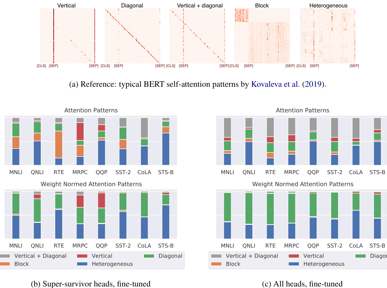
Figure 4: Attention pattern type distribution
图 4: 注意力模式类型分布
The number of block pattern decreased, and we hypothesize that they are now classified as heterogeneous (as they would be unlikely to look diagonal). But even with the normed attention, the utility of super-survivor heads cannot be attributed only to their linguistic functions (especially given that the fraction of heterogeneous patterns is only a rough upper bound). The Pearson’s correlation between heads being super-survivors and their having heterogeneous attention patterns is 0.015 for the raw, and 0.025 for the normed attention. Many “important” heads have diagonal attention patterns, which seems redundant.
块模式的数量减少了,我们假设它们现在被归类为异质模式(因为它们不太可能呈现对角线形态)。但即使经过归一化注意力处理,超级幸存头(super-survivor heads)的效用也不能仅归因于它们的语言功能(特别是考虑到异质模式的比例仅是一个粗略的上限)。原始注意力中超级幸存头与异质注意力模式之间的皮尔逊相关系数为0.015,归一化注意力中为0.025。许多"重要"头具有对角线注意力模式,这似乎存在冗余。
We conducted the same analysis for the attention patterns in pre-trained vs. fine-tuned BERT for both super-survivors and all heads, and found them to not change considerably after fine-tuning, which is consistent with findings by Kovaleva et al. (2019). Full data is available in Appendix F.
我们对预训练和微调后的BERT中超级幸存者(super-survivors)及所有注意力头的注意力模式进行了相同分析,发现微调后其变化不大,这与Kovaleva等人 (2019) 的研究结果一致。完整数据见附录F。
Note that this result does not exclude the possibility that linguistic information is encoded in certain combinations of BERT elements. However, to date most BERT analysis studies focused on the functions of individual components (Voita et al., 2019; Htut et al., 2019; Clark et al., 2019;
需要注意的是,这一结果并不排除BERT元素特定组合中可能编码了语言信息的可能性。然而,迄今为止大多数BERT分析研究都集中在单个组件的功能上 (Voita et al., 2019; Htut et al., 2019; Clark et al., 2019)。
Lin et al., 2019; Vig and Belinkov, 2019; Hewitt and Manning, 2019; Tenney et al., 2019, see also the overview by Rogers et al. (2020b)), and this evidence points to the necessity of looking at their interactions. It also adds to the ongoing discussion of interpret ability of self-attention (Jain and Wallace, 2019; Serrano and Smith, 2019; Wiegreffe and Pinter, 2019; Brunner et al., 2020).
Lin et al., 2019; Vig and Belinkov, 2019; Hewitt and Manning, 2019; Tenney et al., 2019 (另见 Rogers et al. (2020b) 的综述), 这些证据表明有必要研究它们的相互作用。这也为当前关于自注意力 (self-attention) 可解释性的讨论增添了新内容 (Jain and Wallace, 2019; Serrano and Smith, 2019; Wiegreffe and Pinter, 2019; Brunner et al., 2020)。
Once again, he t ero generous pattern counts are only a crude upper bound estimate on potentially interpret able patterns. More sophisticated alternatives should be explored in future work. For instance, the recent information-theoretic probing by minimum description length (Voita and Titov, 2020) avoids the problem of false positives with traditional probing class if i ers.
再次强调,零样本模式计数仅是对潜在可解释模式的粗略上限估计。未来工作中应探索更复杂的替代方法。例如,Voita和Titov (2020) 提出的基于最小描述长度的信息论探测方法,规避了传统探测分类器存在的假阳性问题。
5.3 Information Shared Between Tasks
5.3 任务间共享信息
While the “good” sub networks are not stable, the overlaps between the “good” sub networks may still be used to characterize the tasks themselves. We leave detailed exploration to future work, but as a brief illustration, Figure 5 shows pairwise overlaps in the “good” sub networks for the GLUE tasks.
虽然"优质"子网络并不稳定,但这些子网络之间的重叠部分仍可用于刻画任务本身。我们将详细探索留待未来研究,但作为简要说明,图5展示了GLUE任务中"优质"子网络的两两重叠情况。
The overlaps are not particularly large, but still more than what we would expect if the heads were completely independent (e.g. MRPC and QNLI share over a half of their “good” sub networks). Both heads and MLPs show a similar pattern. Full data for full and super-survivor “good” subnetworks is available in Appendix G.
重叠部分并不特别大,但仍比我们预期的完全独立情况要多(例如 MRPC 和 QNLI 共享了超过一半的"优质"子网络)。注意力头 (head) 和 MLP 都表现出相似的模式。完整数据和超级幸存者"优质"子网络的详细数据见附录 G。

Figure 5: Overlaps in BERT’s “good” sub networks between GLUE tasks: self-attention heads.
图 5: BERT在GLUE任务间"优质"子网络的重叠情况:自注意力头部分
Given our results in subsection 5.2, the overlaps in the “good” sub networks are not explain able by two tasks’ relying on the same linguistic patterns in individual self-attention heads. They also do not seem to depend on the type of the task. For instance, consider the fact that two tasks targeting paraphrases (MRPC and QQP) have less in common than MRPC and MNLI. Alternatively, the overlaps may indicate shared heuristics, or patterns somehow encoded in combinations of BERT elements. This remains to be explored in future work.
根据我们在5.2小节中的结果,"优质"子网络的重叠性无法通过两个任务依赖相同自注意力头中的语言模式来解释。这种重叠似乎也不取决于任务类型。例如,针对释义的两个任务(MRPC和QQP)的共同点反而少于MRPC与MNLI之间的共同点。另一种可能是,这些重叠反映了共享的启发式规则,或是BERT元素组合中编码的某种模式。这仍有待未来研究进一步探索。
6 Discussion
6 讨论
This study confirms the main prediction of LTH for pre-trained BERT weights for both m- and s-pruning. An unexpected finding is that with spruning, the “random” sub networks are still almost as good as the “good” ones, and even the “worst” ones perform on par with a strong baseline. This suggests that the weights that do not survive pruning are not just “inactive” (Zhang et al., 2019).
本研究验证了LTH对预训练BERT权重在m剪枝和s剪枝中的主要预测。一个意外发现是:采用s剪枝时,"随机"子网络的性能仍与"优质"子网络相当,甚至"最差"子网络的表现也能媲美强基线水平。这表明被剪枝剔除的权重并非仅是"非活跃"状态 (Zhang et al., 2019)。
An obvious, but very difficult question that arises from this finding is whether the “bad” sub networks do well because even they contain some linguistic knowledge, or just because GLUE tasks are overall easy and could be learned even by random BERT (Kovaleva et al., 2019), or even any sufficiently large model. Given that we did not find even the “good” sub networks to be stable, or preferentially containing the heads that could have interpret able linguistic functions, the latter seems more likely.
从这一发现引出了一个显而易见但非常困难的问题:这些"糟糕"的子网络表现良好,是因为它们本身也包含某些语言知识,还是仅仅因为GLUE任务整体较为简单,甚至随机BERT [20] 或任何足够大的模型都能学会。鉴于我们甚至没有发现"优秀"子网络具有稳定性,或优先包含那些可能具有可解释语言功能的注意力头 (attention head) ,后一种情况似乎更有可能。
Furthermore, should we perhaps be asking the same question with respect to not only sub networks, but also full models, such as BERT itself and all the follow-up Transformers? There is a trend to automatically credit any new state-of-the-art model with with better knowledge of language. However, what if that is not the case, and the success of pretraining is rather due to the flatter and wider optima in the optimization surface (Hao et al., 2019)? Can similar loss landscapes be obtained from other, non-linguistic pre-training tasks? There are initial results pointing in that direction: Papa dimitri ou and Jurafsky (2020) report that even training on MIDI music is helpful for transfer learning for LM task with LSTMs.
此外,我们是否不仅应该对子网络提出同样的问题,还应该针对完整模型(如 BERT 本身及后续所有 Transformer)提出质疑?当前存在一种趋势,即自动将任何新的最先进模型归功于对语言更好的理解。然而,如果事实并非如此,而预训练的成功反而是由于优化曲面中更平坦、更宽广的最优解(Hao et al., 2019)呢?能否通过其他非语言预训练任务获得类似的损失景观?已有初步研究指向这一方向:Papa dimitri ou 和 Jurafsky (2020) 报告称,即使是 MIDI 音乐训练也有助于 LSTM 在语言模型任务中的迁移学习。
7 Conclusion
7 结论
This study systematically tested the lottery ticket hypothesis in BERT fine-tuning with two pruning methods: magnitude-based weight pruning and importance-based pruning of BERT self-attention heads and MLPs. For both methods, we find that the pruned “good” sub networks alone reach the performance comparable with the full model, while the “bad” ones do not. However, for structured pruning, even the “bad” sub networks can be finetuned separately to reach fairly strong performance. The “good” sub networks are not stable across finetuning runs, and their success is not attributable exclusively to non-trivial linguistic patterns in individual self-attention heads. This suggests that most of pre-trained BERT is potentially useful in fine-tuning, and its success could have more to do with optimization surfaces rather than specific bits of linguistic knowledge.
本研究系统性地验证了彩票假设在BERT微调中的适用性,采用两种剪枝方法:基于权重大小的剪枝和基于重要性的BERT自注意力头与MLP剪枝。实验发现,两种方法剪枝后的"优质"子网络均可达到与完整模型相当的性能,而"劣质"子网络则无法实现。但值得注意的是,对于结构化剪枝,即便"劣质"子网络通过单独微调也能获得较强性能。研究还表明,"优质"子网络在不同微调过程中并不稳定,其成功不能简单归因于单个自注意力头中特定的语言学模式。这表明预训练BERT的大部分参数在微调时都具有潜在效用,其成功可能更多与优化曲面特性相关,而非特定的语言学知识片段。
Carbon Impact Statement. This work contributed $115.644\mathrm{kg}$ of $\mathrm{CO}_{2e q}$ to the atmosphere and used $249.068\mathrm{kWh}$ of electricity, having a NLD-specific social cost of carbon of 
. The social cost of carbon uses models from (Ricke et al., 2018) and this statement and emissions information was generated with experiment-impact-tracker (Henderson et al., 2020).
碳影响声明。本工作向大气排放了115.644千克二氧化碳当量(CO₂eq),消耗了249.068千瓦时电力,其荷兰特定碳社会成本为14美元( -0.24, 0.04 )。碳社会成本采用了(Ricke et al., 2018)的模型,本声明及排放信息通过experiment-impact-tracker (Henderson et al., 2020)生成。
Acknowledgments
致谢
The authors would like to thank Michael Carbin, Aleksandr Drozd, Jonathan Frankle, Naomi Saphra and Sri Ananda Seelan for their helpful comments, the Zoho corporation for providing access to their clusters for running our experiments, and the anonymous reviewers for their insightful reviews and suggestions. This work is funded in part by the NSF award number IIS-1844740 to Anna Rumshisky.
作者感谢Michael Carbin、Aleksandr Drozd、Jonathan Frankle、Naomi Saphra和Sri Ananda Seelan提供的宝贵意见,感谢Zoho公司提供实验集群资源,并感谢匿名评审人的深刻评议与建议。本研究部分资金由美国国家科学基金会(NSF)资助(奖项编号IIS-1844740),受资助人为Anna Rumshisky。
References
参考文献
Jesse Dodge, Gabriel Ilharco, Roy Schwartz, Ali Farhadi, Hannaneh Hajishirzi, and Noah Smith. 2020. Fine-Tuning Pretrained Language Models:
Jesse Dodge、Gabriel Ilharco、Roy Schwartz、Ali Farhadi、Hannaneh Hajishirzi和Noah Smith。2020。微调预训练语言模型:
Weight Initialization s, Data Orders, and Early Stopping. arXiv:2002.06305 [cs].
权重初始化、数据顺序与早停策略。arXiv:2002.06305 [cs]。
W.B. Dolan and C. Brockett. 2005. Automatically constructing a corpus of sentential paraphrases. In Third International Workshop on Paraphrasing (IWP2005). Asia Federation of Natural Language Processing.
W.B. Dolan 和 C. Brockett. 2005. 自动构建句子复述语料库. 第三届国际复述研讨会 (IWP2005). 亚洲自然语言处理联合会.
Jonathan Frankle and Michael Carbin. 2019. The Lottery Ticket Hypothesis: Finding Sparse, Trainable Neural Networks. In International Conference on Learning Representations.
Jonathan Frankle 和 Michael Carbin. 2019. 彩票假设 (The Lottery Ticket Hypothesis): 寻找稀疏可训练的神经网络. In International Conference on Learning Representations.
Danilo Gia m piccolo, Bernardo Magnini, Ido Dagan, and Bill Dolan. 2007. The Third PASCAL Recognizing Textual Entailment Challenge. In Proceedings of the ACL-PASCAL Workshop on Textual Entailment and Paraphrasing, RTE ’07, pages 1–9, Prague, Czech Republic. Association for Computational Linguistics.
Danilo Gia m piccolo、Bernardo Magnini、Ido Dagan和Bill Dolan。2007. 第三届PASCAL文本蕴含识别挑战赛。载于《ACL-PASCAL文本蕴含与复述研讨会论文集》,RTE '07,第1-9页,捷克共和国布拉格。计算语言学协会。
Mitchell A. Gordon, Kevin Duh, and Nicholas Andrews. 2020. Compressing BERT: Studying the effects of weight pruning on transfer learning. ArXiv, abs/2002.08307.
Mitchell A. Gordon、Kevin Duh 和 Nicholas Andrews。2020。压缩 BERT:研究权重剪枝对迁移学习的影响。ArXiv,abs/2002.08307。
R. Bar Haim, Ido Dagan, Bill Dolan, Lisa Ferro, Danilo Gia m piccolo, Bernardo Magnini, and Idan Szpektor. 2006. The Second Pascal Recognising Textual Entailment Challenge. In Proceedings of the Second PASCAL Challenges Workshop on Recognising Textual Entailment.
R. Bar Haim、Ido Dagan、Bill Dolan、Lisa Ferro、Danilo Giampiccolo、Bernardo Magnini和Idan Szpektor。2006。第二届PASCAL文本蕴含识别挑战赛。见《第二届PASCAL文本蕴含识别挑战研讨会论文集》。
Yaru Hao, Li Dong, Furu Wei, and Ke Xu. 2019. Vi- sualizing and Understanding the Effectiveness of BERT. In Proceedings of the 2019 Conference on Empirical Methods in Natural Language Processing and the 9th International Joint Conference on Natural Language Processing (EMNLP-IJCNLP), pages 4143–4152, Hong Kong, China. Association for Computational Linguistics.
Yaru Hao、Li Dong、Furu Wei 和 Ke Xu。2019. 可视化与理解 BERT 的有效性。2019年自然语言处理经验方法会议暨第九届自然语言处理国际联合会议论文集 (EMNLP-IJCNLP),第4143-4152页,中国香港。计算语言学协会。
Peter Henderson, Jieru Hu, Joshua Romoff, Emma Brunskill, Dan Jurafsky, and Joelle Pineau. 2020. Towards the Systematic Reporting of the Energy and Carbon Footprints of Machine Learning. arXiv:2002.05651 [cs].
Peter Henderson、Jieru Hu、Joshua Romoff、Emma Brunskill、Dan Jurafsky 和 Joelle Pineau。2020。机器学习能源与碳足迹的系统化报告方法。arXiv:2002.05651 [cs]。
John Hewitt and Christopher D. Manning. 2019. A Structural Probe for Finding Syntax in Word Represent at ions. In Proceedings of the 2019 Conference of the North American Chapter of the Association for Computational Linguistics: Human Language Technologies, Volume 1 (Long and Short Papers), pages 4129–4138.
John Hewitt 和 Christopher D. Manning. 2019. 一种用于在词表示中寻找句法结构的结构探针. 见《2019年北美计算语言学协会人类语言技术会议论文集》第1卷(长文与短文), 第4129–4138页.
Phu Mon Htut, Jason Phang, Shikha Bordia, and Samuel R Bowman. 2019. Do attention heads in BERT track syntactic dependencies? arXiv preprint arXiv:1911.12246.
Phu Mon Htut, Jason Phang, Shikha Bordia, 和 Samuel R Bowman. 2019. BERT中的注意力头是否跟踪句法依赖关系? arXiv预印本 arXiv:1911.12246.
Sarthak Jain and Byron C. Wallace. 2019. Attention is not Explanation. In Proceedings of the 2019 Conference of the North American Chapter of the Association for Computational Linguistics: Human Language Technologies, Volume 1 (Long and Short Papers), pages 3543–3556.
Sarthak Jain和Byron C. Wallace。2019。《注意力并非解释》。载于《2019年北美计算语言学协会人类语言技术分会会议论文集(长文与短文)》第1卷,第3543–3556页。
Xiaoqi Jiao, Yichun Yin, Lifeng Shang, Xin Jiang, Xiao Chen, Linlin Li, Fang Wang, and Qun Liu. 2019. TinyBERT: Distilling BERT for natural language understanding. arXiv preprint arXiv:1909.10351.
肖琪娇、尹一淳、尚立峰、姜欣、陈晓、李琳琳、王芳和刘群。2019. TinyBERT: 用于自然语言理解的BERT蒸馏方法。arXiv预印本 arXiv:1909.10351。
Di Jin, Zhijing Jin, Joey Tianyi Zhou, and Peter Szolovits. 2020. Is BERT Really Robust? A Strong Baseline for Natural Language Attack on Text Classification and Entailment. In AAAI 2020.
Di Jin、Zhijing Jin、Joey Tianyi Zhou 和 Peter Szolovits。2020。BERT真的鲁棒吗?文本分类与文本蕴含任务的自然语言攻击强基线。发表于AAAI 2020。
Goro Kobayashi, Tatsuki Kuri bay a shi, Sho Yokoi, and Kentaro Inui. 2020. Attention Module is Not Only a Weight: Analyzing Transformers with Vector Norms. arXiv:2004.10102 [cs].
Goro Kobayashi、Tatsuki Kuribayashi、Sho Yokoi和Kentaro Inui。2020。注意力模块不仅是权重:基于向量范数的Transformer分析。arXiv:2004.10102 [cs]。
Olga Kovaleva, Alexey Romanov, Anna Rogers, and Anna Rumshisky. 2019. Revealing the Dark Secrets of BERT. In Proceedings of the 2019 Conference on Empirical Methods in Natural Language Processing and the 9th International Joint Conference on Natural Language Processing (EMNLP-IJCNLP), pages 4356–4365, Hong Kong, China. Association for Computational Linguistics.
Olga Kovaleva、Alexey Romanov、Anna Rogers和Anna Rumshisky。2019。揭示BERT的黑暗秘密。2019年自然语言处理经验方法会议暨第九届自然语言处理国际联合会议论文集(EMNLP-IJCNLP),第4356-4365页,中国香港。计算语言学协会。
Zhenzhong Lan, Mingda Chen, Sebastian Goodman, Kevin Gimpel, Piyush Sharma, and Radu Soricut. 2020. ALBERT: A Lite BERT for Self-Supervised Learning of Language Representations. In ICLR.
Zhenzhong Lan, Mingda Chen, Sebastian Goodman, Kevin Gimpel, Piyush Sharma 和 Radu Soricut. 2020. ALBERT: 一种轻量级BERT用于语言表征的自监督学习. In ICLR.
Namhoon Lee, Thal a i yasin gam Ajanthan, and Philip Torr. 2018. SNIP: Single-shot network pruning based on connection sensitivity. In International Conference on Learning Representations.
Namhoon Lee、Thalaiyasingam Ajanthan 和 Philip Torr。2018. SNIP:基于连接敏感度的单次网络剪枝。In International Conference on Learning Representations。
Hector J Levesque, Ernest Davis, and Leora Morgenstern. 2012. The Winograd Schema Challenge. In Proceedings of the Thirteenth International Conference on Principles of Knowledge Representation and Reasoning, pages 552–561.
Hector J Levesque、Ernest Davis 和 Leora Morgenstern。2012. The Winograd Schema Challenge。载于《第十三届知识表示与推理国际会议论文集》,第552–561页。
Yongjie Lin, Yi Chern Tan, and Robert Frank. 2019. Open Sesame: Getting inside BERT’s Linguistic Knowledge. In Proceedings of the 2019 ACL Workshop Blackbox NLP: Analyzing and Interpreting Neural Networks for NLP, pages 241–253.
Yongjie Lin、Yi Chern Tan和Robert Frank。2019。芝麻开门:探索BERT的语言学知识。2019年ACL研讨会Blackbox NLP论文集:分析与解释神经网络在自然语言处理中的应用,第241-253页。
Nelson F. Liu, Matt Gardner, Yonatan Belinkov, Matthew E. Peters, and Noah A. Smith. 2019. Linguistic Knowledge and Transfer ability of Contextual Representations. In Proceedings of the 2019 Conference of the North American Chapter of the Association for Computational Linguistics: Human Language Technologies, Volume 1 (Long and Short Papers), pages 1073–1094, Minneapolis, Minnesota. Association for Computational Linguistics.
Nelson F. Liu、Matt Gardner、Yonatan Belinkov、Matthew E. Peters 和 Noah A. Smith。2019. 上下文表征的语言知识及迁移能力。载于《2019年北美计算语言学协会人类语言技术会议论文集》第1卷(长文与短文),第1073–1094页,明尼苏达州明尼阿波利斯。计算语言学协会。
JS McCarley. 2019. Pruning a BERT-based Question Answering Model. arXiv preprint arXiv:1910.06360.
JS McCarley. 2019. 基于BERT的问答模型剪枝. arXiv预印本 arXiv:1910.06360.
R. Thomas McCoy, Junghyun Min, and Tal Linzen. 2019a. BERTs of a feather do not generalize together: Large variability in generalization across models with similar test set performance. ArXiv, abs/1911.02969.
R. Thomas McCoy、Junghyun Min 和 Tal Linzen。2019a。同类BERT未必能共同泛化:测试集表现相近的模型间泛化能力存在巨大差异。ArXiv, abs/1911.02969。
Tom McCoy, Ellie Pavlick, and Tal Linzen. 2019b. Right for the Wrong Reasons: Diagnosing Syntactic Heuristics in Natural Language Inference. In Proceedings of the 57th Annual Meeting of the Association for Computational Linguistics, pages 3428– 3448, Florence, Italy. Association for Computational Linguistics.
Tom McCoy、Ellie Pavlick和Tal Linzen。2019b。《正确的错误原因:自然语言推理中句法启发式的诊断》。载于《第57届计算语言学协会年会论文集》,第3428-3448页,意大利佛罗伦萨。计算语言学协会。
Paul Michel, Omer Levy, and Graham Neubig. 2019. Are Sixteen Heads Really Better than One? Advances in Neural Information Processing Systems 32 (NIPS 2019).
Paul Michel、Omer Levy 和 Graham Neubig。2019。多头注意力机制真的比单头更好吗?《神经信息处理系统进展》32卷 (NIPS 2019)。
Pavlo Molchanov, Stephen Tyree, Tero Karras, Timo Aila, and Jan Kautz. 2017. Pruning convolutional neural networks for resource efficient inference. In 5th International Conference on Learning Representations, ICLR 2017, Toulon, France, April 24- 26, 2017, Conference Track Proceedings. OpenReview.net.
Pavlo Molchanov、Stephen Tyree、Tero Karras、Timo Aila 和 Jan Kautz。2017. 面向资源高效推理的卷积神经网络剪枝技术。载于《第五届国际学习表征会议(ICLR 2017)会议论文集》,2017年4月24-26日,法国土伦。OpenReview.net。
Ari Morcos, Haonan Yu, Michela Paganini, and Yuandong Tian. 2019. One ticket to win them all: Generalizing lottery ticket initialization s across datasets and optimizers. In Advances in Neural Information Processing Systems 32, pages 4932–4942. Curran Associates, Inc.
Ari Morcos、Haonan Yu、Michela Paganini和Yuandong Tian。2019。一券通赢:彩票初始化方法在数据集和优化器间的泛化性研究。载于《神经信息处理系统进展》第32卷,第4932–4942页。Curran Associates公司。
Timothy Niven and Hung-Yu Kao. 2019. Probing Neural Network Comprehension of Natural Language Arguments. In Proceedings of the 57th Annual Meeting of the Association for Computational Linguistics, pages 4658–4664, Florence, Italy. Association for Computational Linguistics.
Timothy Niven 和 Hung-Yu Kao。2019。探究神经网络对自然语言论证的理解。在《第57届计算语言学协会年会论文集》中,第4658-4664页,意大利佛罗伦萨。计算语言学协会。
Isabel Papa dimitri ou and Dan Jurafsky. 2020. Learning Music Helps You Read: Using Transfer to Study Linguistic Structure in Language Models. arXiv:2004.14601 [cs].
Isabel Papa dimitri ou 和 Dan Jurafsky. 2020. 学习音乐有助于阅读:利用迁移研究语言模型中的语言结构. arXiv:2004.14601 [cs].
Pranav Rajpurkar, Jian Zhang, Konstantin Lopyrev, and Percy Liang. 2016. SQuAD: $100{,}000+$ Questions for Machine Comprehension of Text. In Proceedings of the 2016 Conference on Empirical Methods in Natural Language Processing, pages 2383–2392. Association for Computational Linguistics.
Pranav Rajpurkar、Jian Zhang、Konstantin Lopyrev 和 Percy Liang。2016. SQuAD:面向机器理解文本的 $100{,}000+$ 问题。载于《2016年自然语言处理实证方法会议论文集》,第2383–2392页。计算语言学协会。
Katharine Ricke, Laurent Drouet, Ken Caldeira, and Massimo Tavoni. 2018. Country-level social cost of carbon. Nature Climate Change, 8(10):895.
Katharine Ricke、Laurent Drouet、Ken Caldeira 和 Massimo Tavoni。2018。国家层面的碳社会成本。《自然-气候变化》8(10):895。
Anna Rogers, Olga Kovaleva, Matthew Downey, and Anna Rumshisky. 2020a. Getting Closer to AI Complete Question Answering: A Set of Prerequisite Real Tasks. In AAAI, page 11.
Anna Rogers、Olga Kovaleva、Matthew Downey 和 Anna Rumshisky. 2020a. 迈向 AI 完备问答: 一组先决现实任务. 见 AAAI, 第 11 页.
Anna Rogers, Olga Kovaleva, and Anna Rumshisky. 2020b. A Primer in BERTology: What we know about how BERT works. arXiv:2002.12327 [cs].
Anna Rogers、Olga Kovaleva 和 Anna Rumshisky。2020b。BERTology 入门:我们对 BERT 工作原理的认知。arXiv:2002.12327 [cs]。
Victor Sanh, Lysandre Debut, Julien Chaumond, and Thomas Wolf. 2019. DistilBERT, a distilled version of BERT: Smaller, faster, cheaper and lighter. In 5th Workshop on Energy Efficient Machine Learning and Cognitive Computing - NeurIPS 2019.
Victor Sanh、Lysandre Debut、Julien Chaumond和Thomas Wolf。2019。DistilBERT:BERT的精简版——更小、更快、更经济、更轻量。发表于《第五届高效节能机器学习与认知计算研讨会 - NeurIPS 2019》。
Sofia Serrano and Noah A. Smith. 2019. Is Attention Interpret able? arXiv:1906.03731 [cs].
Sofia Serrano和Noah A. Smith. 2019. 注意力机制可解释吗? arXiv:1906.03731 [cs].
Richard Socher, Alex Perelygin, Jean Wu, Jason Chuang, Christopher D. Manning, Andrew Ng, and Christopher Potts. 2013. Recursive deep models for semantic compositional it y over a sentiment treebank. In Proceedings of the 2013 Conference on Empirical Methods in Natural Language Processing, pages 1631–1642.
Richard Socher、Alex Perelygin、Jean Wu、Jason Chuang、Christopher D. Manning、Andrew Ng 和 Christopher Potts。2013。基于情感树库的语义组合性递归深度模型。载于《2013年自然语言处理实证方法会议论文集》,第1631–1642页。
Nitish Srivastava, Geoffrey E. Hinton, Alex Krizhevsky, Ilya Sutskever, and Ruslan Salakhutdinov. 2014. Dropout: a simple way to prevent neural networks from over fitting. J. Mach. Learn. Res., 15:1929–1958.
Nitish Srivastava、Geoffrey E. Hinton、Alex Krizhevsky、Ilya Sutskever 和 Ruslan Salakhutdinov。2014。Dropout: 一种防止神经网络过拟合的简单方法。《机器学习研究杂志》,15:1929–1958。
Ian Tenney, Dipanjan Das, and Ellie Pavlick. 2019. BERT Rediscovers the Classical NLP Pipeline. In Proceedings of the 57th Annual Meeting of the Association for Computational Linguistics, pages 4593– 4601.
Ian Tenney、Dipanjan Das和Ellie Pavlick。2019。BERT重拾经典自然语言处理流程。载于《第57届计算语言学协会年会论文集》,第4593–4601页。
Ashish Vaswani, Noam Shazeer, Niki Parmar, Jakob Uszkoreit, Llion Jones, Aidan N. Gomez, Lukasz Kaiser, and Illia Polosukhin. 2017. Attention is all you need. In NIPS, pages 5998–6008, Long Beach, CA, USA.
Ashish Vaswani、Noam Shazeer、Niki Parmar、Jakob Uszkoreit、Llion Jones、Aidan N. Gomez、Lukasz Kaiser 和 Illia Polosukhin。2017. Attention is all you need。载于《NIPS》,第5998-6008页,美国加州长滩。
Jesse Vig and Yonatan Belinkov. 2019. Analyzing the Structure of Attention in a Transformer Language Model. In Proceedings of the 2019 ACL Workshop Blackbox NLP: Analyzing and Interpreting Neural Networks for NLP, pages 63–76, Florence, Italy. Association for Computational Linguistics.
Jesse Vig 和 Yonatan Belinkov。2019。分析Transformer语言模型中的注意力结构。2019年ACL黑盒NLP研讨会论文集:分析与解释自然语言处理神经网络,第63-76页,意大利佛罗伦萨。计算语言学协会。
Elena Voita, David Talbot, Fedor Moiseev, Rico Sen- nrich, and Ivan Titov. 2019. Analyzing Multi-Head Self-Attention: Specialized Heads Do the Heavy Lifting, the Rest Can Be Pruned. In Proceedings of the 57th Annual Meeting of the Association for Computational Linguistics, pages 5797–5808, Florence, Italy. Association for Computational Linguistics.
Elena Voita、David Talbot、Fedor Moiseev、Rico Sennrich和Ivan Titov。2019。多头自注意力机制分析:专用头承担重任,其余可被剪枝。载于《第57届计算语言学协会年会论文集》,第5797–5808页,意大利佛罗伦萨。计算语言学协会。
Elena Voita and Ivan Titov. 2020. InformationTheoretic Probing with Minimum Description Length. arXiv:2003.12298 [cs].
Elena Voita 和 Ivan Titov. 2020. 基于最小描述长度的信息论探测方法. arXiv:2003.12298 [cs].
Alex Wang, Amapreet Singh, Julian Michael, Felix Hill, Omer Levy, and Samuel R. Bowman. 2018. GLUE: A Multi-Task Benchmark and Analysis Platform for Natural Language Understanding. In Proceedings of the 2018 EMNLP Workshop BlackboxNLP: Analyzing and Interpreting Neural Networks for NLP, pages 353–355, Brussels, Belgium. Association for Computational Linguistics.
Alex Wang、Amapreet Singh、Julian Michael、Felix Hill、Omer Levy 和 Samuel R. Bowman。2018. GLUE:自然语言理解的多任务基准与分析平台。载于《2018年EMNLP研讨会BlackboxNLP:分析与解释自然语言处理神经网络论文集》,第353–355页,比利时布鲁塞尔。计算语言学协会。
Alex Warstadt, Amanpreet Singh, and Samuel R. Bowman. 2019. Neural Network Acceptability Judgments. Transactions of the Association for Computational Linguistics, 7:625–641.
Alex Warstadt、Amanpreet Singh和Samuel R. Bowman。2019。神经网络可接受性判断。计算语言学协会汇刊,7:625–641。
Sarah Wiegreffe and Yuval Pinter. 2019. Attention is not not Explanation. In Proceedings of the 2019 Conference on Empirical Methods in Natural Language Processing and the 9th International Joint Conference on Natural Language Processing (EMNLP-IJCNLP), pages 11–20, Hong Kong, China. Association for Computational Linguistics.
Sarah Wiegreffe 和 Yuval Pinter. 2019. 注意力并非不是解释。 2019年自然语言处理经验方法会议暨第九届自然语言处理国际联合会议论文集 (EMNLP-IJCNLP), 第11-20页, 中国香港. 计算语言学协会。
Adina Williams, Nikita Nangia, and Samuel R. Bowman. 2017. A Broad-Coverage Challenge Corpus for Sentence Understanding through Inference. In Proceedings of the 2018 Conference of the North American Chapter of the Association for Computational Linguistics: Human Language Technologies, Volume 1 (Long Papers), pages 1112–1122, New Orleans, Louisiana. Association for Computational Linguistics.
Adina Williams、Nikita Nangia和Samuel R. Bowman。2017. 面向广泛覆盖的句子理解推理挑战语料库。载于《2018年北美计算语言学协会人类语言技术会议论文集(长论文)》第1卷,第1112-1122页,美国路易斯安那州新奥尔良。计算语言学协会。
Thomas Wolf, Lysandre Debut, Victor Sanh, Julien Chaumond, Clement Delangue, Anthony Moi, Pier- ric Cistac, Tim Rault, Rémi Louf, Morgan Funtow- icz, and Jamie Brew. 2020. Hugging Face’s Transformers: State-of-the-art Natural Language Processing. arXiv:1910.03771 [cs].
Thomas Wolf、Lysandre Debut、Victor Sanh、Julien Chaumond、Clement Delangue、Anthony Moi、Pier-ric Cistac、Tim Rault、Rémi Louf、Morgan Funtowicz 和 Jamie Brew。2020. Hugging Face的Transformers:最先进的自然语言处理技术。arXiv:1910.03771 [cs]。
Haonan Yu, Sergey Edunov, Yuandong Tian, and Ari S. Morcos. 2020. Playing the lottery with rewards and multiple languages: Lottery tickets in RL and NLP. In ICLR.
Haonan Yu、Sergey Edunov、Yuandong Tian 和 Ari S. Morcos。2020。用奖励和多语言玩彩票:强化学习与自然语言处理中的彩票假设。发表于 ICLR。
Rowan Zellers, Ari Holtzman, Yonatan Bisk, Ali Farhadi, and Yejin Choi. 2019. HellaSwag: Can a Machine Really Finish Your Sentence? In ACL 2019.
Rowan Zellers、Ari Holtzman、Yonatan Bisk、Ali Farhadi和Yejin Choi。2019. HellaSwag:机器真能完成你的句子吗?见ACL 2019。
Chiyuan Zhang, Samy Bengio, and Yoram Singer. 2019. Are All Layers Created Equal? In ICML 2019 Workshop Deep Phenomena.
张驰远、Samy Bengio 和 Yoram Singer。2019。《所有层生而平等吗?》收录于 ICML 2019 研讨会《深度现象》。
Hattie Zhou, Janice Lan, Rosanne Liu, and Jason Yosinski. 2019. De constructing Lottery Tickets: Zeros, Signs, and the Supermask. In Advances in Neural Information Processing Systems 32, pages 3597–3607. Curran Associates, Inc.
Hattie Zhou、Janice Lan、Rosanne Liu和Jason Yosinski。2019。解构彩票假设:零值、符号与超级掩码。载于《神经信息处理系统进展》第32卷,第3597–3607页。Curran Associates公司。
A “Good” Sub networks in BERT Fine-tuned on GLUE Tasks
BERT在GLUE任务微调中的"优质"子网络
Each figure in this section shows the “good” subnetwork of heads and layers that survived the pruning process described in section 3. Each task was run with 5 different random seeds. The top number in each cell indicates how likely a given head or MLP was to survive pruning, with 1.0 indicating that it survived on every run. The bottom number indicates the standard deviation across runs.
本节中的每个图表都展示了经过第3节所述剪枝过程后存留的"优质"子网络中的注意力头和层。每项任务均使用5个不同的随机种子运行。单元格顶部数字表示给定注意力头或MLP存活于剪枝的概率,1.0表示每次运行均存活。底部数字表示各次运行的标准差。
The figures in this appendix show that each task has a varying number of heads and layers that survive pruning on all fine-tuning runs, while some heads and layers were only “picked up” by some random seeds. Note also that in addition to the architecture elements that survive across many runs, there are also some that are useful for over half of the tasks, as shown in Figure 15, and some always survive the pruning.
本附录中的图表显示,每项任务在剪枝后保留的注意力头(attention head)和网络层(layer)数量各不相同,其中部分头与层仅被某些随机种子"选中"。还需注意的是,除在多轮训练中持续保留的架构元素外,如图15所示,有些元素对超半数任务有效,另一些则始终能通过剪枝。
Visualizing the “good” subnetwork illustrates the core problem with WNLI, the most difficult task of GLUE. Figure 14 shows that each run is completely different, indicating that BERT fails to find any consistent pattern between the task and the information in the available pre-trained weights. WNLI is described as “somewhat adversarial” by Wang et al. (2018) because it has similar sentences in train and dev sets with opposite labels.
可视化"优质"子网络揭示了WNLI的核心问题,这是GLUE基准中最具挑战性的任务。图14显示每次运行结果都截然不同,表明BERT无法在任务与预训练权重信息之间找到任何一致性模式。Wang等人 (2018) 将WNLI描述为"具有一定对抗性",因为其在训练集和开发集中包含标签相反但语句相似的样本。

Figure 6: MNLI
图 6: MNLI

Figure 7: QNLI
图 7: QNLI

Figure 8: RTE
图 8: RTE

Figure 9: MRPC
图 9: MRPC

Figure 10: QQP
图 10: QQP

Figure 11: SST-2
图 11: SST-2

Figure 12: CoLA
图 12: CoLA

Figure 13: STS-B
图 13: STS-B

Figure 14: WNLI
图 14: WNLI
B Iterative Pruning Modes
B 迭代剪枝模式
We conducted additional experiments with the following settings for iterative pruning based on importance scores:
我们基于重要性分数进行了以下设置的迭代剪枝补充实验:
• Heads only: in each iteration, we mask as many of the unmasked heads with the lowest importance scores as we can (144 heads in the full BERT-base model).
• 仅限注意力头:在每次迭代中,我们会尽可能多地屏蔽掉重要性分数最低的未屏蔽注意力头(在完整的BERT-base模型中共有144个注意力头)。
• MLPs only: we iterative ly mask one of the remaining MLPs that has the smallest importance score (subsection 3.3).
• 仅限MLP:我们迭代地屏蔽剩余MLPs中重要性分数最小的一个(第3.3节)。
• Heads and $M L P s$ : we compute head (sub- section 3.3) and MLP (subsection 3.3) impor- tance scores in a single backward pass, pruning $10%$ heads and one MLP with the smallest scores until the performance on the dev set is within $90%$ . Then we continue pruning heads alone, and then MLPs alone. This strategy results in a larger number of total components pruned within our performance threshold.
• 注意力头和MLP层:我们通过单次反向传播计算注意力头(见第3.3节)和MLP层(见第3.3节)的重要性分数,依次剪枝重要性分数最低的10%注意力头和一个MLP层,直到开发集性能保持在90%以上。随后单独剪枝注意力头,再单独剪枝MLP层。该策略使我们能在性能阈值内剪枝更多组件。

Figure 15: The “good” sub networks: self-attention heads and MLPs that survive pruning. Each cell gives the average number of GLUE tasks in which a given head/MLP survived, and the standard deviation across 5 finetuning initialization s.
图 15: "优质"子网络:剪枝后保留的自注意力头(self-attention heads)和MLP。每个单元格显示给定头/MLP在GLUE任务中存活的平均数量,以及5次微调初始化的标准差。
(d) Surviving MLPs (masking heads and MLPs)
(d) 存活的MLP (掩蔽注意力头和MLP)
| 0.56 ± 0.00 WNLI | 0.34 ± 0.06 | 0.54 ± 0.06 0.80 ± 0.01 | 0.54 ± 0.06 0.54 ± 0.06 | 0.54 ± 0.06 0.79 ± 0.08 | 0.54 ± 0.06 0.54 ± 0.06 0.32 ± 0.38 0.61 ± 0.21 | 0.54 ± 0.06 0.56 ± 0.00 | 0.54 ± 0.06 | 0.56 ± 0.00 0.54 ± 0.06 | 0.56 ± 0.00 | 0.48 ± 0.10 0.82 ± 0.02 | 0.41 ± 0.11 0.88 ± 0.00 | 0.51 ± 0.08 0.08 ± 0.04 | 0.47 ± 0.12 0.24 ± 0.03 | 0.53 ± 0.06 0.05 ± 0.07 | 0.49 ± 0.11 | 0.08 ± 0.00 | ||||||
| 0.02 ± 0.00 STS-B | 0.89 ± 0.00 | 0.84 ± 0.01 | 0.75 ± 0.23 0.53 ± 0.25 0.87 ± 0.07 0.69 ± 0.13 | 0.89 ± 0.01 | 0.62 ± 0.15 | 0.86 ± 0.06 | 0.38 ± 0.07 0.80 ± 0.00 0.54 ± 0.03 0.84 ± 0.00 | 0.06 ± 0.06 0.50 ± 0.01 | 0.12 ± 0.03 0.85 ± 0.00 | 0.06 ± 0.02 0.51 ± 0.02 | 0.13 ± 0.01 0.83 ± 0.01 | 0.85 ± 0.01 | 0.92 ± 0.00 | 0.55 ± 0.09 | 0.83 ± 0.01 | 0.49 ± 0.01 | 0.82 ± 0.00 | |||||
| 0.51 ± 0.00 SST-2 | 0.93 ± 0.00 | 0.57 ± 0.03 | 0.58 ± 0.06 | 0.51 ± 0.04 | 0.56 ± 0.05 | 0.49 ± 0.04 | 0.59 ± 0.04 | 0.52 ± 0.02 | 0.50 ± 0.03 | 0.47 ± 0.00 0.50 ± 0.03 | 0.52 ± 0.02 | 0.49 ± 0.03 | 0.61 ± 0.01 | 0.61 ± 0.02 | 0.47 ± 0.00 | 0.56 ± 0.02 | 0.49 ± 0.03 0.49 ± 0.03 | |||||
| 0.53 ± 0.00 RTE | 0.63 ± 0.03 | 0.83 ± 0.01 0.89 ± 0.01 | 0.74 ± 0.07 | 0.88 ± 0.03 | 0.68 ± 0.06 0.82 ± 0.11 | 0.63 ± 0.00 0.87 ± 0.00 | 0.63 ± 0.00 | 0.83 ± 0.04 | 0.60 ± 0.07 | 0.87 ± 0.00 | 0.83 ± 0.01 | 0.91 ± 0.00 | 0.63 ± 0.00 | 0.86 ± 0.00 | 0.63 ± 0.00 | 0.78 ± 0.00 | ||||||
| QQP | 0.63 ± 0.00 0.91 ± 0.00 0.92 ± 0.00 | S-pruning Subnetworks | 0.83 ± 0.00 0.89 ± 0.02 | 0.69 ± 0.12 | 0.84 ± 0.05 | 0.63 ± 0.06 0.77 ± 0.12 | 0.56 ± 0.03 0.83 ± 0.00 | 0.50 ± 0.01 | 0.76 ± 0.08 | 0.49 ± 0.02 | 0.57 ± 0.03 | M-pruning Subnetworks | 0.84 ± 0.01 | 0.91 ± 0.00 | 0.51 ± 0.02 | 0.81 ± 0.01 | 0.51 ± 0.02 0.61 ± 0.00 | |||||
| 0.51 ± 0.00 0.68 ± 0.00 | 0.84 ± 0.01 | 0.77 ± 0.01 0.77 ± 0.06 | 0.48 ± 0.23 | 0.68 ± 0.21 | 0.43 ± 0.15 | 0.68 ± 0.14 | 0.39 ± 0.16 0.71 ± 0.00 | 0.39 ± 0.16 | 0.69 ± 0.01 | 0.39 ± 0.16 | 0.69 ± 0.01 | 0.78 ± 0.02 | 0.84 ± 0.01 | 0.39 ± 0.16 | 0.70 ± 0.01 | 0.39 ± 0.16 | 0.68 ± 0.01 | |||||
| MNLI | 0.35 ± 0.00 | 0.84 ± 0.00 | 0.76 ± 0.00 0.80 ± 0.04 | 0.64 ± 0.19 | 0.79 ± 0.08 | 0.60 ± 0.13 | 0.80 ± 0.05 | 0.34 ± 0.01 | 0.76 ± 0.00 0.32 ± 0.01 | 0.75 ± 0.01 | 0.32 ± 0.00 | 0.77 ± 0.00 | 0.78 ± 0.00 | 0.84 ± 0.00 | 0.33 ± 0.01 | 0.76 ± 0.00 | 0.32 ± 0.00 | 0.62 ± 0.00 | ||||
| CoLA | 0.00 ± 0.00 | 0.51 ± 0.01 | 0.50 ± 0.04 | 0.43 ± 0.11 | 0.42 ± 0.23 | 0.34 ± 0.09 | 0.41 ± 0.11 | 0.13 ± 0.06 0.49 ± 0.02 | 0.02 ± 0.05 | 0.15 ± 0.15 | 0.01 ± 0.01 | 0.13 ± 0.03 | 0.52 ± 0.01 0.54 ± 0.02 | 0.02 ± 0.03 | 0.16 ± 0.06 | 0.00 ± 0.00 | 0.02 ± 0.03 | |||||
| Experiment | 0.56 ± 0.01 majority baseline full model | (pounid) ,poos, | random (pruned) | random (retrained) (pounid) peq, | "bad’ (retrained) | ’(pruned) poos, | random (pruned) | random (retrained) | (paund) peq, | “bad’ (retrained) | (paunid) poos, | (retrained) .poos, | random (pruned) | random (retrained) | “bad’ (retrained) (paund) peq, |
| 0.56 ± 0.00 WNLI | 0.34 ± 0.06 | 0.54 ± 0.06 0.80 ± 0.01 | 0.54 ± 0.06 0.54 ± 0.06 | | 0.54 ± 0.06 0.79 ± 0.08 | 0.54 ± 0.06 0.54 ± 0.06 0.32 ± 0.38 0.61 ± 0.21 | | 0.54 ± 0.06 0.56 ± 0.00 | 0.54 ± 0.06 | | 0.56 ± 0.00 0.54 ± 0.06 | 0.56 ± 0.00 | | 0.48 ± 0.10 0.82 ± 0.02 | 0.41 ± 0.11 0.88 ± 0.00 | 0.51 ± 0.08 0.08 ± 0.04 | 0.47 ± 0.12 0.24 ± 0.03 | 0.53 ± 0.06 0.05 ± 0.07 | 0.49 ± 0.11 | 0.08 ± 0.00 | |
| 0.02 ± 0.00 STS-B | 0.89 ± 0.00 | 0.84 ± 0.01 | 0.75 ± 0.23 0.53 ± 0.25 0.87 ± 0.07 0.69 ± 0.13 | 0.89 ± 0.01 | | 0.62 ± 0.15 | 0.86 ± 0.06 | 0.38 ± 0.07 0.80 ± 0.00 0.54 ± 0.03 0.84 ± 0.00 | 0.06 ± 0.06 0.50 ± 0.01 | 0.12 ± 0.03 0.85 ± 0.00 | 0.06 ± 0.02 0.51 ± 0.02 | 0.13 ± 0.01 0.83 ± 0.01 | | 0.85 ± 0.01 | 0.92 ± 0.00 | 0.55 ± 0.09 | 0.83 ± 0.01 | 0.49 ± 0.01 | 0.82 ± 0.00 | |
| 0.51 ± 0.00 SST-2 | 0.93 ± 0.00 | 0.57 ± 0.03 | 0.58 ± 0.06 | 0.51 ± 0.04 | 0.56 ± 0.05 | 0.49 ± 0.04 | 0.59 ± 0.04 | 0.52 ± 0.02 | 0.50 ± 0.03 | 0.47 ± 0.00 0.50 ± 0.03 | | 0.52 ± 0.02 | 0.49 ± 0.03 | 0.61 ± 0.01 | 0.61 ± 0.02 | 0.47 ± 0.00 | | 0.56 ± 0.02 | 0.49 ± 0.03 0.49 ± 0.03 | |
| 0.53 ± 0.00 RTE | 0.63 ± 0.03 | | 0.83 ± 0.01 0.89 ± 0.01 | 0.74 ± 0.07 | | 0.88 ± 0.03 | 0.68 ± 0.06 0.82 ± 0.11 | | 0.63 ± 0.00 0.87 ± 0.00 | 0.63 ± 0.00 | 0.83 ± 0.04 | 0.60 ± 0.07 | 0.87 ± 0.00 | | 0.83 ± 0.01 | 0.91 ± 0.00 | 0.63 ± 0.00 | 0.86 ± 0.00 | 0.63 ± 0.00 | 0.78 ± 0.00 |
| QQP | 0.63 ± 0.00 0.91 ± 0.00 0.92 ± 0.00 | S-pruning Subnetworks | 0.83 ± 0.00 0.89 ± 0.02 | 0.69 ± 0.12 | | 0.84 ± 0.05 | 0.63 ± 0.06 0.77 ± 0.12 | | 0.56 ± 0.03 0.83 ± 0.00 | 0.50 ± 0.01 | 0.76 ± 0.08 | 0.49 ± 0.02 | 0.57 ± 0.03 | M-pruning Subnetworks | 0.84 ± 0.01 | 0.91 ± 0.00 | 0.51 ± 0.02 | 0.81 ± 0.01 | | 0.51 ± 0.02 0.61 ± 0.00 |
| | 0.51 ± 0.00 0.68 ± 0.00 | 0.84 ± 0.01 | 0.77 ± 0.01 0.77 ± 0.06 | 0.48 ± 0.23 | | 0.68 ± 0.21 | 0.43 ± 0.15 | 0.68 ± 0.14 | 0.39 ± 0.16 0.71 ± 0.00 | 0.39 ± 0.16 | 0.69 ± 0.01 | 0.39 ± 0.16 | 0.69 ± 0.01 | | 0.78 ± 0.02 | 0.84 ± 0.01 | 0.39 ± 0.16 | 0.70 ± 0.01 | 0.39 ± 0.16 | 0.68 ± 0.01 |
| MNLI | 0.35 ± 0.00 | 0.84 ± 0.00 | 0.76 ± 0.00 0.80 ± 0.04 | 0.64 ± 0.19 | | 0.79 ± 0.08 | 0.60 ± 0.13 | 0.80 ± 0.05 | 0.34 ± 0.01 | 0.76 ± 0.00 0.32 ± 0.01 | 0.75 ± 0.01 | 0.32 ± 0.00 | 0.77 ± 0.00 | | 0.78 ± 0.00 | 0.84 ± 0.00 | 0.33 ± 0.01 | 0.76 ± 0.00 | 0.32 ± 0.00 | 0.62 ± 0.00 |
| CoLA | 0.00 ± 0.00 | | 0.51 ± 0.01 | 0.50 ± 0.04 | 0.43 ± 0.11 | 0.42 ± 0.23 | 0.34 ± 0.09 | 0.41 ± 0.11 | | 0.13 ± 0.06 0.49 ± 0.02 | 0.02 ± 0.05 | 0.15 ± 0.15 | 0.01 ± 0.01 | 0.13 ± 0.03 | | 0.52 ± 0.01 0.54 ± 0.02 | 0.02 ± 0.03 | 0.16 ± 0.06 | 0.00 ± 0.00 | 0.02 ± 0.03 |
| Experiment | 0.56 ± 0.01 majority baseline full model | | (pounid) ,poos, | | random (pruned) | | random (retrained) (pounid) peq, | "bad’ (retrained) | | ’(pruned) poos, | random (pruned) | random (retrained) | (paund) peq, | "bad’ (retrained) | | (paunid) poos, | (retrained) .poos, | random (pruned) | random (retrained) | "bad’ (retrained) (paund) peq, |
D Longer Fine-tuning of “Bad” s-pruned Sub networks
| Epoch | CoLA | SST-2 | MRPC | QQP | STS-B | MNLI | QNLI | RTE | WNLI | Avg |
| 3 | 0.422 | 0.873 | 0.71 | 0.832 | 0.651 | 0.805 | 0.764 | 0.579 | 0.498 | 0.6815 |
| 4 | 0.423 | 0.859 | 0.663 | 0.828 | 0.652 | 0.804 | 0.762 | 0.587 | 0.554 | 0.6813 |
| 5 | 0.432 | 0.862 | 0.665 | 0.831 | 0.668 | 0.801 | 0.752 | 0.590 | 0.523 | 0.6804 |
| 6 | 0.425 | 0.867 | 0.655 | 0.830 | 0.667 | 0.800 | 0.753 | 0.594 | 0.521 | 0.6791 |
D 对"不良"s剪枝子网络进行更长时间微调
| Epoch | CoLA | SST-2 | MRPC | QQP | STS-B | MNLI | QNLI | RTE | WNLI | Avg |
|---|---|---|---|---|---|---|---|---|---|---|
| 3 | 0.422 | 0.873 | 0.71 | 0.832 | 0.651 | 0.805 | 0.764 | 0.579 | 0.498 | 0.6815 |
| 4 | 0.423 | 0.859 | 0.663 | 0.828 | 0.652 | 0.804 | 0.762 | 0.587 | 0.554 | 0.6813 |
| 5 | 0.432 | 0.862 | 0.665 | 0.831 | 0.668 | 0.801 | 0.752 | 0.590 | 0.523 | 0.6804 |
| 6 | 0.425 | 0.867 | 0.655 | 0.830 | 0.667 | 0.800 | 0.753 | 0.594 | 0.521 | 0.6791 |
E Performance of the “Super Survivor” Sub networks
E "超级幸存者"子网络的性能
In this experiment, we explore three settings:
在本实验中,我们探索了三种设置:
“good” sub networks: the sub networks consisting only of “super-survivors”: the selfattention heads and MLPs that survived in all random seeds, shown in Appendix A. These sub networks are much smaller than the pruned sub networks discussed in subsection 4.2 (10- $30%$ vs $50%$ of the full model);
优质子网络:仅由"超级幸存者"构成的子网络:即在所有随机种子中都存留下来的自注意力头和MLP(多层感知机),详见附录A。这些子网络规模远小于第4.2节讨论的剪枝后子网络(占完整模型的10-30% vs 50%);
• “bad” sub networks: the sub networks the same size as the super-survivor sub networks, but selected from heads and MLPs the least likely to survive importance pruning;
• "坏"子网络:与超级幸存子网络大小相同,但从最不可能在重要性剪枝中存活的注意力头和MLP中选取的子网络;
random sub networks: same size as supersurvivor sub networks, but selected from elements that were neither super-survivors, nor the ones in the “bad” sub networks.
随机子网络:与超存子网络大小相同,但从不属于超存子网络或"不良"子网络的元素中选取。
The striking conclusion is that on 6 out of 9 tasks the bad and random sub networks behaved nearly as well as the “good” ones, suggesting that the “supersurvivor” self-attention heads and MLPs did not survive importance pruning because of their encoding some unique linguistic information necessary for solving the GLUE tasks.
一个惊人的结论是,在9项任务中有6项任务上,表现差和随机的子网络表现几乎与"好"子网络相当,这表明那些"超级幸存"的自注意力头和MLP之所以未在重要性剪枝中幸存,并非因为它们编码了解决GLUE任务所需的独特语言信息。

Figure 17: The performance of “super survivor” sub networks in BERT fine-tuning: performance on GLUE tasks (error bars indicate standard deviation across 5 fine-tuning runs). The size of the super-survivor subnetwork as $%$ of full model weights is shown next to the task names.
图 17: BERT微调中"超级幸存者"子网络的性能表现:在GLUE任务上的性能(误差条表示5次微调运行的标准差)。超级幸存者子网络规模占完整模型权重的百分比显示在任务名称旁边。
F Attention Pattern Type Distribution
F 注意力模式类型分布
We use two separately trained CNN class if i ers to analyze the BERT’s self-attention maps, both “raw” head outputs and weight-normed attention, following Kobayashi et al. (2020). For the former, we use 400 annotated maps by Kovaleva et al. (2019), and for the latter we additionally annotate 600 more maps.
我们使用两个独立训练的CNN分类器来分析BERT的自注意力图,包括"原始"头部输出和权重归一化后的注意力,遵循Kobayashi等人(2020)的方法。对于前者,我们使用Kovaleva等人(2019)标注的400张图,对于后者我们额外标注了600张图。
We run the class if i ers on pre-trained and fine-tuned
我们在预训练和微调模型上运行分类器
BERT, both the full model and the model pruned by the “super-survivor” mask (only the heads and MLPs that survived across GLUE tasks). For each experiment, we report the fraction of attention patterns estimated from a hundred dev-set samples for each task across five random seeds.
BERT,包括完整模型和通过"超级幸存者"掩码剪枝后的模型(仅保留在GLUE任务中存活的注意力头和MLP层)。每个实验报告中,我们基于五个随机种子,统计了从每个任务的一百个开发集样本中估算出的注意力模式占比。
See Figure 4a for attention types illustration.
见图 4a: 注意力类型示意图。

Figure 18: Attention pattern distribution in all BERT self-attention heads and the “super-survivor” heads.
图 18: 所有BERT自注意力头中的注意力模式分布及"超级幸存者"头。
G How Task-independent are the “Good” Sub networks?
G 这些“优质”子网络的任务无关性如何?
The parts of the “good” sub networks that are only relevant for some specific tasks, but consistently survive across fine-tuning runs for that task, should encode the information useful for that task, even if it is not deeply linguistic. Therefore, the degree to which the “good” sub networks overlap across tasks may be a useful way to characterize the tasks themselves.
“好”子网络中仅与某些特定任务相关、但在该任务微调过程中持续保留的部分,应该编码了对该任务有用的信息——即使这些信息并非深层语言学特征。因此,不同任务间“好”子网络的重叠程度,或许能成为表征任务本质的有效方式。
Figure 19 shows pairwise comparisons between all GLUE tasks with respect to the number of shared heads and MLPs in two conditions: the “good” subnetworks found by structured importance pruning that were described in subsection 4.1, and supersurvivors (the heads/MLPs that survived in all random seeds).
图 19: 展示了两种条件下所有GLUE任务之间关于共享注意力头(shared heads)和MLP数量的成对比较:4.1小节所述通过结构化重要性剪枝(structured importance pruning)找到的"优质"子网络,以及超幸存者(supersurvivors) (在所有随机种子中都存活的注意力头/MLPs)。

Figure 19: The “good” subnetwork: The diagonal represents the BERT architecture components that survive pruning for a given task and remaining elements represent the common surviving components across GLUE tasks. Each cell gives the average number of heads (out of 144) or layers (out of 12), together with standard deviation across 5 random initialization s (for (a) and (b)).
图 19: "优质"子网络:对角线表示针对特定任务剪枝后保留的 BERT 架构组件,其余元素代表跨 GLUE 任务共同保留的组件。每个单元格显示平均保留的注意力头数量(共 144 个)或层数(共 12 层),以及 5 次随机初始化的标准差(适用于 (a) 和 (b))。