Uncertainty Inspired RGB-D Saliency Detection

不确定性启发的RGB-D显著性检测

Abstract—We propose the first stochastic framework to employ uncertainty for RGB-D saliency detection by learning from the data labeling process. Existing RGB-D saliency detection models treat this task as a point estimation problem by predicting a single saliency map following a deterministic learning pipeline. We argue that, however, the deterministic solution is relatively ill-posed. Inspired by the saliency data labeling process, we propose a generative architecture to achieve probabilistic RGB-D saliency detection which utilizes a latent variable to model the labeling variations. Our framework includes two main models: 1) a generator model, which maps the input image and latent variable to stochastic saliency prediction, and 2) an inference model, which gradually updates the latent variable by sampling it from the true or approximate posterior distribution. The generator model is an encoder-decoder saliency network. To infer the latent variable, we introduce two different solutions: i) a Conditional Variation al Auto-encoder with an extra encoder to approximate the posterior distribution of the latent variable; and ii) an Alternating Back-Propagation technique, which directly samples the latent variable from the true posterior distribution. Qualitative and quantitative results on six challenging RGB-D benchmark datasets show our approach’s superior performance in learning the distribution of saliency maps. The source code is publicly available via our project page: https://github.com/Jing Zhang 617/UCNet.

摘要—我们首次提出通过从数据标注过程中学习，利用不确定性进行RGB-D显著性检测的随机框架。现有RGB-D显著性检测模型遵循确定性学习流程，通过预测单一显著性图将该任务视为点估计问题。然而，我们认为确定性解决方案存在相对不适定性。受显著性数据标注过程启发，我们提出一种生成式架构来实现概率化RGB-D显著性检测，该架构利用潜变量建模标注差异。我们的框架包含两个主要模型：1) 生成器模型，将输入图像和潜变量映射为随机显著性预测；2) 推理模型，通过从真实或近似后验分布中采样来逐步更新潜变量。生成器模型采用编码器-解码器结构的显著性网络。针对潜变量推断，我们引入两种解决方案：i) 条件变分自编码器，通过额外编码器逼近潜变量的后验分布；ii) 交替反向传播技术，直接从真实后验分布中采样潜变量。在六个具有挑战性的RGB-D基准数据集上的定性与定量结果表明，我们的方法在学习显著性图分布方面具有卓越性能。源代码已通过项目页面公开：https://github.com/JingZhang617/UCNet。

Index Terms—Uncertainty, RGB-D Saliency Prediction, Conditional Variation al Auto encoders, Alternating Back-Propagation.

索引术语—不确定性、RGB-D显著性预测、条件变分自编码器 (Conditional Variational Autoencoders)、交替反向传播 (Alternating Back-Propagation)。

1 INTRODUCTION

1 引言

BJECT-level saliency detection (i.e., salient object detection) O involves separating the most conspicuous objects that attract human attention from the background [2]–[9]. Recently, visual saliency detection from RGB-D images has attracted lots of interests due to the importance of depth information in the human vision system and the popularity of depth sensing technologies [1], [10]–[15]. With the extra depth data, conventional RGB-D saliency detection models focus on predicting one single saliency map for the RGB-D input by exploring the complementary information between the RGB image and the depth data.

物体级显著性检测（即显著物体检测）O 涉及将最引人注目、吸引人类注意的物体从背景中分离出来 [2]–[9]。近年来，由于深度信息在人类视觉系统中的重要性以及深度传感技术的普及，基于 RGB-D 图像的视觉显著性检测引起了广泛关注 [1], [10]–[15]。借助额外的深度数据，传统 RGB-D 显著性检测模型通过探索 RGB 图像与深度数据之间的互补信息，专注于为 RGB-D 输入预测单一的显著性图。

The standard practice for RGB-D saliency detection is to train a deep neural network using ground-truth (GT) saliency maps provided by the corresponding benchmark datasets, thus formulating saliency detection as a point estimation problem by learning a mapping function $Y=f(X;\theta)$ , where $\theta$ represents network parameter set, and $X$ and $Y$ are input RGB-D image pair and corresponding GT saliency map. Usually, the GT saliency maps are obtained through human consensus or by the dataset creators [16]. Building upon large scale RGB-D datasets, deep convolutional neural network-based RGB-D saliency detection models [10], [11], [14], [17], [18] have made profound progress. We argue that the way RGB-D saliency detection progresses through the conventional pipelines [10], [11], [14], [17], [18] fails to capture the uncertainty in labeling the GT saliency maps.

RGB-D显著性检测的标准做法是使用基准数据集提供的真实标注(GT)显著性图训练深度神经网络，从而通过学习映射函数$Y=f(X;\theta)$将显著性检测表述为点估计问题，其中$\theta$表示网络参数集，$X$和$Y$分别代表输入的RGB-D图像对及其对应的GT显著性图。通常，GT显著性图通过人工共识或数据集创建者标注获得[16]。基于大规模RGB-D数据集，采用深度卷积神经网络的RGB-D显著性检测模型[10][11][14][17][18]已取得显著进展。我们认为，传统流程[10][11][14][17][18]推进RGB-D显著性检测的方式未能捕捉GT显著性图标注过程中的不确定性。

According to research in human visual perception [19], visual saliency detection is subjective to some extent. Each person could have specific preferences [20] in labeling the saliency map (which has been discussed in user-specific saliency detection [21]). More precisely speaking, the GT labeling process is never a deterministic process, which is different from category-aware tasks, such as semantic segmentation [22], as a “Table” will never be ambiguously labeled as “Cat”, while the salient foreground for one annotator may be defined as background by other annotators as shown in the second row of Fig. 1.

根据人类视觉感知研究[19]，视觉显著性检测在一定程度上具有主观性。每个人在标注显著性图时可能存在特定偏好[20]（这一问题已在用户特异性显著性检测[21]中讨论过）。更准确地说，真实标注(GT)过程绝非确定性过程，这与语义分割[22]等类别感知任务不同——例如"桌子"永远不会被模糊标注为"猫"，而如图1 第二行所示，某标注者定义的显著前景可能被其他标注者判定为背景。

In Fig. 1, we present the GT saliency map and other candidate salient regions (produced by our CVAE-based method, which will be introduced in Section 3.2) that may attract human attention. Fig. 1 shows that the deterministic mapping (from “Image” to “GT”) may lead to an “over-confident” model, as the provided “GT” may be biased as shown in the second row of Fig. 1. To overcome this, instead of performing point estimation, we are interested in how the network achieves distribution estimation with diverse saliency maps produced1, capturing the uncertainty of human annotation. Furthermore, in practice, it is more desirable to have multiple saliency maps produced to reflect human uncertainty instead of a single saliency map prediction for subsequent tasks.

在图1中，我们展示了GT显著性图（ground truth）及其他可能吸引人类注意的候选显著区域（由我们基于CVAE的方法生成，该方法将在3.2节介绍）。图1表明，确定性映射（从"图像"到"GT"）可能导致模型"过度自信"，如图1第二行所示，所提供的"GT"可能存在偏差。为解决这个问题，我们关注网络如何通过生成多样化的显著性图来实现分布估计，从而捕捉人类标注的不确定性。此外，在实际应用中，为后续任务生成多个反映人类不确定性的显著性图，比单一显著性图预测更具实用价值。

Inspired by human perceptual uncertainty, as well as the labeling process of saliency maps, we propose a generative architecture to achieve probabilistic RGB-D saliency detection with a latent variable $z$ modeling human uncertainty in the annotation. Two main models are included in this framework: 1) a generator (i.e., encoder-decoder) model, which maps the input RGB-D data and latent variable to stochastic saliency prediction; and 2) an inference model, which progressively refreshes the latent variable.

受到人类感知不确定性以及显著性图标注过程的启发，我们提出了一种生成式架构，通过潜在变量 $z$ 建模标注过程中的人类不确定性，实现概率化的RGB-D显著性检测。该框架包含两个主要模型：1) 生成器（即编码器-解码器）模型，将输入RGB-D数据和潜在变量映射为随机显著性预测；2) 推理模型，逐步更新潜在变量。

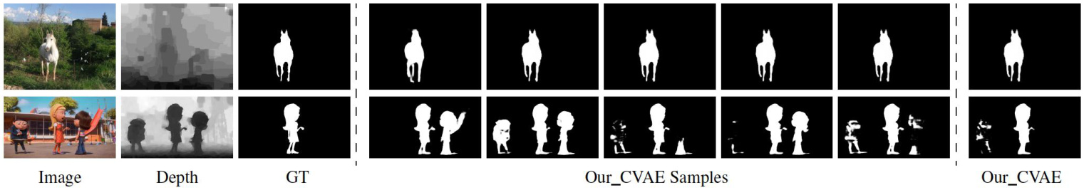
Fig. 1. GT compared with our predicted saliency maps. For simple context image (first row), we can produce consistent predictions. When dealing with complex scenarios where there exists uncertainties in salient regions (second row), our model can produce diverse predictions (“Our CVAE Samples”), where “Our CVAE” is our deterministic prediction after the saliency consensus module, which will be introduced in Section 3.3.

图 1: GT与我们的预测显著性图对比。对于简单上下文图像(第一行)，我们能生成一致的预测结果。当处理存在显著性区域不确定性的复杂场景时(第二行)，我们的模型可以生成多样化预测("Our CVAE Samples")，其中"Our CVAE"是经过显著性共识模块后的确定性预测结果(详见第3.3节)。

To infer the latent variable, we introduce two different strategies:

为了推断潜在变量，我们引入了两种不同的策略：

A Conditional Variation al Auto-encoder (CVAE) [23] based model with an additional encoder to approximate the posterior distribution of the latent variable. The Alternating Back-Propagation (ABP) [24] based technique, which directly samples the latent variable from the true posterior distribution via Langevin Dynamics based Markov chain Monte Carlo (MCMC) sampling [25], [26].

基于条件变分自编码器(CVAE) [23]的模型，额外增加一个编码器来近似潜在变量的后验分布。基于交替反向传播(ABP) [24]的技术，通过基于朗之万动力学的马尔可夫链蒙特卡洛(MCMC)采样 [25][26]直接从真实后验分布中采样潜在变量。

This paper is an extended version of our conference paper, UCNet [1]. In particular, UC-Net focuses on generating saliency maps via CVAE and augmented ground-truth to model diversity and to avoid posterior collapse problem [27]. While UC-Net showed promising performance by modeling such variations, it still has a number of shortcomings. Firstly, UC-Net requires engineering efforts (ground-truth augmentation) to model diversity and achieve stabilized training (mitigating posterior collapse). Here, we use a simpler technique to achieve the same goal, by using the standard KL-annealing strategy [28], [29] with less human intervention. Experimental results in Fig. 13 clearly illustrate the effectiveness of the KL-annealing strategy. Secondly, we improve the quality of the generated saliency maps by designing a more expressive decoder that benefits from spatial and channel attention mechanisms [30]. Thirdly, inspired by [23] we modify the cost function of UC-Net to reduce the discrepancy in encoding the latent variable at training and test time, which is elaborated in Section 3.

本文是我们会议论文UCNet [1]的扩展版本。具体而言，UC-Net专注于通过CVAE和增强的真实标注数据生成显著性图，以建模多样性并避免后验坍塌问题[27]。虽然UC-Net通过建模这些变化展现了良好的性能，但仍存在一些不足。首先，UC-Net需要人工设计（真实标注数据增强）来建模多样性并实现稳定训练（缓解后验坍塌）。本文采用更简单的KL退火策略[28][29]达成相同目标，减少了人为干预。图13的实验结果清晰证明了KL退火策略的有效性。其次，我们通过设计具有空间和通道注意力机制[30]的更强大解码器，提升了生成显著性图的质量。第三，受[23]启发，我们修改了UC-Net的损失函数以减少训练和测试时潜在变量编码的差异，详见第3节。

Moreover, CVAE-based methods approximate the posterior distribution via an inference model (or an encoder) and optimize the evidence lower bound (ELBO). The lower bound is simply the composition of the reconstruction loss and the divergence between the approximate posterior and prior distribution. If the model focuses more on optimizing the reconstruction quality, the latent space may fail to learn meaningful representation. On the other hand, if the model focuses more on reducing the divergence between the approximate posterior and prior distribution, the model may sacrifice the reconstruction quality. Additionally, since the model approximates the posterior distribution rather than modeling the true posterior, it may lose expressivity in general. Here, we propose to use Alternating Back-Propagation (ABP) technique [24] that directly samples latent variables from the true posterior. While it is much simpler, our experimental results show ABP leads to impressive result for generating saliency maps. Note that both CVAE-based and ABP-based solutions can produce stochastic saliency predictions by modeling output space distribution as a generative model conditioned on the input RGB-D image pair. Similar to UC-Net, during the testing phase, a saliency consensus module is introduced to mimic the majority voting mechanism for GT saliency map generation, and generate one single saliency map in the end for performance evaluation. Finally, in addition to producing state-of-the-art results, our experiments provide a thorough evaluation of the different components of our model as well as an extensive study on the diversity of the generated saliency maps.

此外，基于CVAE的方法通过推理模型（或编码器）近似后验分布，并优化证据下界（ELBO）。该下界由重构损失和近似后验与先验分布之间的散度简单组合而成。若模型更侧重优化重构质量，潜在空间可能无法学习到有意义的表征；反之，若更侧重缩小近似后验与先验分布的差异，则可能牺牲重构质量。此外，由于模型仅近似后验分布而非建模真实后验，其表达能力可能受限。为此，我们提出采用交替反向传播（ABP）技术[24]，直接从真实后验中采样潜在变量。尽管方法更为简洁，实验表明ABP在生成显著图方面效果显著。需注意，基于CVAE和ABP的解决方案均可通过将输出空间分布建模为输入RGB-D图像对的条件生成模型，实现随机显著预测。与UC-Net类似，测试阶段引入显著共识模块模拟GT显著图生成中的多数投票机制，最终生成单张显著图用于性能评估。除取得最优结果外，我们的实验还对模型各组件进行了全面评估，并对生成显著图的多样性展开了深入研究。

Our main contributions are summarized as: 1) We propose the first uncertainty inspired probabilistic RGB-D saliency prediction model with a latent variable $z$ introduced to the network to represent human uncertainty in annotation; 2) We introduce two different schemes to infer the latent variable, including a CVAE [23] framework with an additional encoder to approximate the posterior distribution of $z$ and an ABP [24] pipeline, which samples the latent variable directly from its true posterior distribution via Langevin dynamics based Markov chain Monte Carlo (MCMC) sampling [26]. Each of them can model the conditional distribution of output, and lead to diverse predictions during testing; 3) Extensive experimental results on six RGB-D saliency detection benchmark datasets demonstrate the effectiveness of our proposed solutions.

我们的主要贡献总结如下：1) 我们提出了首个基于不确定性的概率式RGB-D显著性预测模型，通过向网络引入潜在变量 $z$ 来表示人工标注中的不确定性；2) 我们提出了两种不同的潜在变量推断方案：包括采用额外编码器近似 $z$ 后验分布的CVAE [23]框架，以及通过基于Langevin动力学的马尔可夫链蒙特卡洛(MCMC)采样 [26] 直接从真实后验分布中采样潜在变量的ABP [24]流程。这两种方案都能建模输出的条件分布，并在测试阶段生成多样化预测；3) 在六个RGB-D显著性检测基准数据集上的大量实验结果验证了所提方案的有效性。

2 相关工作

In this section, we first briefly review existing RGB-D saliency detection models. We then investigate existing generative models, including Variation al Auto-encoder (VAE) [23], [31], and Generative Adversarial Networks (GAN) [32], [33]. We also highlight the uniqueness of the proposed solutions in this section.

在本节中，我们首先简要回顾现有的RGB-D显著性检测模型。接着探讨现有生成模型，包括变分自编码器(VAE) [23][31]和生成对抗网络(GAN) [32][33]。最后着重阐述本节所提解决方案的独特性。

2.1 RGB-D Saliency Detection

2.1 RGB-D显著性检测

Depending on how the complementary information of RGB images and depth data is fused, existing RGB-D saliency detection models can be roughly classified into three categories: earlyfusion models [1], [34], late-fusion models [18], [35] and crosslevel fusion models [10]–[15], [17], [36]–[43]. The first solution directly concatenates the RGB image with its depth information, forming a four-channel input, and feed it to the network to obtain both the appearance information and geometric information. [34] proposed an early-fusion model to generate features for each superpixel of the RGB-D pair, which was then fed to a CNN to produce saliency of each superpixel. The second approach treats each modality independently, and predictions from both modalities are fused at the end of the network. [35] introduced a late-fusion network (i.e., AFNet) to fuse predictions from the RGB and depth branch adaptively. In a similar pipeline, [18] fused the RGB and depth information through fully connected layers. The third one fuses intermediate features of each modality by considering correlations of the above two modalities. To achieve this, [36] presented a complementary-aware fusion block. [17] designed attention-aware cross-level combination blocks to obtain complementary information of each modality. [11] employed a fluid pyramid integration framework to achieve multi-scale crossmodal feature fusion. [13] designed a self-mutual attention model to effectively fuse RGB and depth information. Similarly, [12] presented a complimentary interaction module (CIM) to select complementary representation from the RGB and depth data. [14] provided joint learning and densely-cooperative fusion framework for complementary feature discovery. [15] introduced a depth distiller to transfer the depth knowledge from the depth stream to the RGB stream to achieve a lightweight architecture without use of depth data at test time. A comprehensive survey can be found in [44].

根据RGB图像与深度数据互补信息的融合方式，现有RGB-D显著性检测模型大致可分为三类：早期融合模型 [1]、[34]，晚期融合模型 [18]、[35] 以及跨层级融合模型 [10]–[15]、[17]、[36]–[43]。第一种方案将RGB图像与其深度信息直接拼接为四通道输入，馈入网络以同时获取外观信息与几何信息。[34] 提出早期融合模型为RGB-D图像对的每个超像素生成特征，再通过CNN计算各超像素的显著性。第二种方案独立处理各模态数据，在网络末端融合双模态预测结果。[35] 提出自适应融合网络（AFNet）动态融合RGB与深度分支的预测；类似地，[18] 通过全连接层融合RGB与深度信息。第三种方案通过考量双模态关联性融合其中间特征。[36] 设计了互补感知融合模块；[17] 采用注意力感知的跨层级组合块获取各模态互补信息；[11] 使用流体金字塔集成框架实现多尺度跨模态特征融合；[13] 构建自互注意力模型有效融合RGB与深度数据；[12] 提出互补交互模块（CIM）从RGB-D数据中筛选互补表征；[14] 开发联合学习与密集协作融合框架用于互补特征发现；[15] 设计深度蒸馏器将深度流知识迁移至RGB流，实现测试阶段无需深度数据的轻量化架构。更全面的综述可参阅 [44]。

2.2 VAE or CVAE-based Deep Probabilistic Models

2.2 基于VAE或CVAE的深度概率模型

Ever since the seminal work by Kingma et al. [31] and Rezende et al. [45], VAE and its conditional counterpart CVAE [23] have been widely applied in various computer vision problems. A typical VAE-based model consists of an encoder, a decoder, and a loss function. The encoder is a neural network with weights and biases $\theta$ , which maps the input datapoint $X$ to a latent (hidden) representation $z$ . The decoder is another neural network with weights and biases $\phi$ , which reconstructs the datapoint $X$ from $z$ . To train a VAE, a reconstruction loss and a regularize r are needed to penalize the disagreement of the latent representation’s prior and posterior distribution. Instead of defining the prior distribution of the latent representation as a standard Gaussian distribution, CVAE-based networks utilize the input observation to modulate the prior on Gaussian latent variables to generate the output.

自Kingma等人[31]和Rezende等人[45]的开创性工作以来，变分自编码器(VAE)及其条件变体CVAE[23]已被广泛应用于各类计算机视觉问题。典型的基于VAE的模型由编码器、解码器和损失函数组成。编码器是具有权重$\theta$的神经网络，将输入数据点$X$映射到潜在表示$z$；解码器是具有权重$\phi$的另一神经网络，负责从$z$重构数据点$X$。训练VAE时需要重构损失和正则项，以惩罚潜在表示先验分布与后验分布的不匹配。与将潜在表示先验定义为标准高斯分布不同，基于CVAE的网络利用输入观测值调制高斯潜在变量的先验分布来生成输出。

In low-level vision, VAE and CVAE have been applied to tasks such as latent representations with sharp samples [46], difference of motion modes [47], medical image segmentation models [48], and modeling inherent ambiguities of an image [49]. Meanwhile, VAE and CVAE have been explored in more complex vision tasks such as uncertain future forecast [50], salient feature enhancement [51], human motion prediction [52], [53], and shape-guided image generation [54]. Recently, VAE and CVAE have been extended to 3D domain targeting applications such as 3D meshes deformation [55], and point cloud instance segmentation [56]. For saliency detection, [57] adopted VAE to model image background, and separated salient objects from the background through the reconstruction residuals.

在低级视觉任务中，变分自编码器 (VAE) 和条件变分自编码器 (CVAE) 已被应用于以下领域：生成清晰样本的潜在表示 [46]、运动模式差异分析 [47]、医学图像分割模型 [48] 以及图像固有模糊性建模 [49]。同时，这两种方法还被探索用于更复杂的视觉任务，包括不确定性未来预测 [50]、显著特征增强 [51]、人体运动预测 [52][53] 以及形状引导的图像生成 [54]。近期，VAE 和 CVAE 进一步扩展到三维领域，应用于三维网格变形 [55] 和点云实例分割 [56] 等场景。在显著性检测方面，[57] 采用 VAE 对图像背景建模，并通过重建残差实现显著对象与背景的分离。

2.3 GAN or CGAN-based Dense Models

2.3 基于GAN或CGAN的密集模型

GAN [32] and its conditional counterparts [33] have also been used in dense prediction tasks. Existing GAN-based dense prediction models mainly focus on two directions: 1) using GANs in a fully supervised manner [58]–[62] and treat the disc rim in at or loss as a higher-order regularize r for dense prediction; or 2) apply GANs to ‘semi-supervised scenarios [63], [64], where the output of the disc rim in at or serves as guidance to evaluate the degree of the unsupervised sample participating in network training. In saliency detection, following the first direction, [65] introduced a disc rim in at or in the fixation prediction network to distinguish predicted fixation map and ground-truth. Different from the above two directions, [66] adopted GAN in a RGB-D saliency detection network to explore the intra-modality (RGB, depth) and crossmodality simultaneously. [67] used GAN as a denoising technique to clear up the noisy input images. [62] designed a disc rim in at or to distinguish real saliency map (group truth) and fake saliency map (prediction), thus structural information can be learned without CRF [68] as post-processing technique. [69] adopted CycleGAN [70] as an domain adaption technique to generate pseudo-NIR image for existing RGB saliency dataset and achieve multispectral image salient object detection.

GAN [32] 及其条件变体 [33] 也被用于密集预测任务。现有基于GAN的密集预测模型主要聚焦两个方向：1) 在全监督模式下使用GAN [58]–[62]，将判别器损失作为密集预测的高阶正则化项；2) 将GAN应用于半监督场景 [63][64]，通过判别器输出来评估无监督样本参与网络训练的程度。在显著性检测领域，[65] 沿袭第一个方向，在注视点预测网络中引入判别器来区分预测注视图与真实标注。不同于上述两种思路，[66] 在RGB-D显著性检测网络中同时探索模态内(RGB/深度)与跨模态特征，[67] 将GAN作为去噪技术净化输入图像噪声。[62] 设计判别器区分真实显著图(标注)与伪造显著图(预测)，从而无需CRF [68] 后处理即可学习结构信息。[69] 采用CycleGAN [70] 作为域适应技术，为现有RGB显著性数据集生成伪近红外图像，实现多光谱图像显著目标检测。

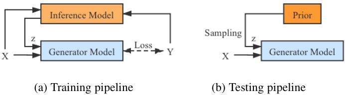
Fig. 2. Training and testing pipeline. During training, the inferred latent variable $z$ and input image $X$ are fed to the “Generator Model” for stochastic saliency prediction. During testing, we sample from the prior distribution of $z$ to produce diverse predictions for each input image.

图 2: 训练与测试流程。训练阶段，推断出的潜在变量 $z$ 和输入图像 $X$ 被输入至"生成器模型 (Generator Model)"进行随机显著性预测。测试阶段，我们从 $z$ 的先验分布中采样，为每张输入图像生成多样化预测结果。

2.4 Uniqueness of Our Solutions

2.4 我们解决方案的独特性

To the best of our knowledge, generative models have not been exploited in saliency detection to model annotation uncertainty, except for our preliminary version [1]. As a conditional latent variable model, two different solutions can be used to infer the latent variable. One is CVAE-based [23] method (the one we used in the preliminary version [1]), which infers the latent variable using Variation al Inference, and another one is MCMC based method, which we propose to use in this work. Specifically, we present a new latent variable inference solution with less parameter load based on the alternating back-propagation technique [24].

据我们所知，除我们的初步版本[1]外，生成式模型尚未被用于显著性检测中以建模标注不确定性。作为条件潜变量模型，可采用两种不同方案推断潜变量：一种是基于CVAE[23]的方法（即我们在初步版本[1]中采用的方案），通过变分推断求解潜变量；另一种是我们本文提出的基于MCMC的方案。具体而言，我们基于交替反向传播技术[24]提出了一种参数负载更小的新潜变量推断方案。

CVAE-based models infer the latent variable through finding the ELBO of the log-likelihood to avoid MCMC as it was too slow in the non-deep-learning era. In other words, CVAEs approximates Maximum Likelihood Estimation (MLE) by finding the ELBO with an extra encoder. The main issue of this strategy is “posterior collapse” [27], where the latent variable is independent of network prediction, making it unable to represent the uncertainty of human annotation. We introduced the “New Label Generation” strategy in our preliminary version [1] as an effective way to avoid posterior collapse problem. In this extended version, we propose a much simpler strategy using the KL annealing strategy [28], [29], which slowly introduces the KL loss term to the loss function with an extra weight. The experimental results show that this simple strategy can avoid the posterior collapse problem with the provided single GT saliency map.

基于CVAE的模型通过寻找对数似然的ELBO来推断潜在变量，以避免MCMC（在非深度学习时代速度过慢）。换言之，CVAE通过额外编码器寻找ELBO来近似最大似然估计（MLE）。该策略的主要问题是"后验坍缩" [27]，即潜在变量与网络预测无关，导致其无法表示人工标注的不确定性。我们在初版论文[1]中提出了"新标签生成"策略作为避免后验坍缩的有效方法。在本扩展版本中，我们采用更简单的KL退火策略[28][29]，通过额外权重逐步将KL损失项引入损失函数。实验结果表明，这种简单策略能在提供单一GT显著性图的情况下避免后验坍缩问题。

Besides the KL annealing term, we introduce ABP [24] as an alternative solution to prevent posterior collapse in the network. ABP introduces gradient-based MCMC and updates the latent variable with gradient descent back-propagation to directly train the network targeting MLE. Compared with CVAE, ABP samples latent variables directly from its true posterior distribution, making it more accurate in inferring the latent variable. Furthermore, no assistant network (the additional encoder in CVAE) used in ABP, which leads to smaller network parameter load.

除了KL退火项外，我们引入ABP [24]作为防止网络后验坍塌的替代方案。ABP采用基于梯度的MCMC方法，通过梯度下降反向传播更新潜变量，直接针对最大似然估计(MLE)训练网络。与CVAE相比，ABP直接从真实后验分布中采样潜变量，使其在推断潜变量时更准确。此外，ABP无需使用辅助网络(CVAE中的额外编码器)，因此网络参数量更小。

We introduce ABP-based inference model as an extension to the CVAE-based pipeline [1]. Experimental results show that both solutions can effectively estimate the latent variable, leading to stochastic saliency predictions. Details of the two inference models are introduced in Section 3.2.

我们引入基于ABP的推理模型作为对基于CVAE的流程[1]的扩展。实验结果表明，这两种方案都能有效估计潜在变量，从而实现随机显著性预测。第3.2节将详细介绍这两种推理模型。

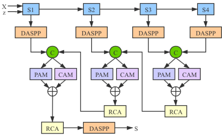
Fig. 3. Details of the “Generator Model”, which takes image $X$ and latent variable $z$ as input, and produce stochastic saliency map $S$ , where $^{\mathrm{{4}}}\mathsf{S}1$ - ${\mathsf{S}}4"$ represent the four convolutional blocks of our backbone network. “DASPP” is the DenseASPP module [71], “PAM” and $\because{\mathsf{C A M}}^{}$ are position attention and channel attention module [30], “RCA” is the Residual Channel Attention operation from [72].

图 3: "生成器模型 (Generator Model)" 的细节，该模型以图像 $X$ 和潜变量 $z$ 作为输入，生成随机显著性图 $S$。其中 $^{\mathrm{{4}}}\mathsf{S}1$ - ${\mathsf{S}}4"$ 表示主干网络的四个卷积块。"DASPP" 是 DenseASPP 模块 [71]，"PAM" 和 $\because{\mathsf{C A M}}^{}$ 分别是位置注意力模块和通道注意力模块 [30]，"RCA" 是来自 [72] 的残差通道注意力操作。

3 OUR MODEL

3 我们的模型

In this section, we present our probabilistic RGB-D saliency detection model, which learns the underlying conditional distribution of saliency maps rather than a mapping function from RGB-D input to a single saliency map. Let $\mathbf{\mathcal{D}}^{\mathrm{~~}}={X_{i},Y_{i}}{i=1}^{N}$ be the training dataset, where $X_{i}$ denotes the RGB-D input, $Y_{i}$ denotes the GT saliency map, and $N$ denotes the total number of images in the dataset. We intend to model $P_{\omega}(Y|X,z)$ , where $z$ is a latent variable representing the inherent uncertainty in salient regions which can be also seen in how a human annotates salient objects. Our framework utilizes two main components during training: 1) a generator model, which maps input RGB-D $X$ and latent variable $z$ to conditional prediction $P_{\omega}(Y|X,z)$ ; and 2) an inference model, which infers the latent variable $z$ . During testing, we can sample multiple latent variables from the learned prior distribution $P_{\theta}(z|X)$ to produce stochastic saliency prediction. The whole pipeline of our model during training and testing is illustrated in Fig. 2 (a) and (b) respectively. Specifically, during training, the model learns saliency from the “Generator Model”, and updates the latent variable with the “Inference Model”. During testing, we sample from the “Prior” distribution of the latent variable to obtain stochastic saliency predictions.

在本节中，我们提出了一种概率化RGB-D显著性检测模型，该模型学习显著性图的基础条件分布，而非从RGB-D输入到单一显著性图的映射函数。令 $\mathbf{\mathcal{D}}^{\mathrm{~~}}={X_{i},Y_{i}}{i=1}^{N}$ 表示训练数据集，其中 $X_{i}$ 代表RGB-D输入，$Y_{i}$ 代表真实显著性图，$N$ 表示数据集中图像总数。我们旨在建模 $P_{\omega}(Y|X,z)$ ，其中 $z$ 是表示显著区域固有不确定性的潜变量，这种不确定性也体现在人工标注显著对象的过程中。我们的框架在训练时采用两个主要组件：1) 生成器模型，将输入RGB-D $X$ 和潜变量 $z$ 映射到条件预测 $P_{\omega}(Y|X,z)$ ；2) 推理模型，用于推断潜变量 $z$ 。测试时，我们可以从学习到的先验分布 $P_{\theta}(z|X)$ 中采样多个潜变量，以生成随机显著性预测。图2(a)和(b)分别展示了训练和测试阶段的整体流程。具体而言，训练时模型通过"生成器模型"学习显著性，并通过"推理模型"更新潜变量；测试时则从潜变量的"先验"分布中采样，获得随机显著性预测。

3.1 Generator Model

3.1 生成器模型

The Generator Model takes $X$ and latent variable $z$ as input, and produces stochastic prediction $S=P_{\omega}(Y|X,z)$ , where $\omega$ is the parameter set of the generator model. We choose ResNet50 [73] as our backbone, which contains four convolutional blocks. To enlarge the receptive field, we follow DenseASPP [71] to obtain a feature map with the receptive field of the whole image on each stage of the backbone network. We then gradually concatenate the two adjacent feature maps in a top-down manner and feed it to a “Residual Channel Attention” module [72] to obtain stochastic saliency map $S$ . As illustrated in Fig. 3, our generator model follows the recent progress in dense prediction problems such as semantic segmentation [22], via a proper use of a hybrid attention mechanism. To this end, our generator model benefits from two types of attention: a Position Attention Module [30] and a Channel Attention Module [30]. The former aims to capture the spatial dependencies between any two locations of the feature map, while the latter aims to capture the channel dependencies between any two channel in the feature map. We follow [30] to aggregate and fuse the outputs of these two attention modules to further enhance the feature representations.

生成器模型以 $X$ 和潜变量 $z$ 为输入，生成随机预测 $S=P_{\omega}(Y|X,z)$ ，其中 $\omega$ 是生成器模型的参数集。我们选择 ResNet50 [73] 作为主干网络，它包含四个卷积块。为了扩大感受野，我们采用 DenseASPP [71] 的方法，在主干网络的每个阶段获取覆盖整张图像感受野的特征图。随后，我们以自上而下的方式逐步拼接相邻两个特征图，并将其输入"残差通道注意力"模块 [72] 以生成随机显著图 $S$ 。如图 3 所示，我们的生成器模型借鉴了语义分割 [22] 等密集预测问题的最新进展，通过合理使用混合注意力机制实现。为此，我们的生成器模型采用两种注意力机制：位置注意力模块 [30] 和通道注意力模块 [30] 。前者用于捕捉特征图中任意两个位置间的空间依赖关系，后者则用于捕捉特征图中任意两个通道间的通道依赖关系。我们按照 [30] 的方法聚合并融合这两个注意力模块的输出，以进一步增强特征表示。

3.2 Inference Model

3.2 推理模型

We propose two different solutions to infer or update the latent variable $z;~1$ ) A CVAE-based [23] pipeline, in which we approximate the posterior distribution via a neural network (i.e., the encoder); and 2) An ABP [24] based strategy to sample directly from the true posterior distribution of $z$ via Langevin Dynamics based MCMC [25].

我们提出两种不同的解决方案来推断或更新潜在变量 $z$：1) 基于CVAE [23] 的流程，通过神经网络（即编码器）近似后验分布；2) 基于ABP [24] 的策略，通过基于朗之万动力学的MCMC [25] 直接从 $z$ 的真实后验分布中采样。

Infer $z$ with CVAE: The Variation al Auto-encoder [31] is a directed graphical model and typically comprise of two fundamental components, an encoder that maps the input variable $X$ to the latent space $Q_{\phi}(z|X)$ , where $z$ is a low dimensional Gaussian variable and a decoder that reconstructs $X$ from $z$ to get $P_{\omega}(X|z)$ . To train the VAE, a reconstruction loss and a regularize r to penalize the disagreement of the prior and the approximate posterior distribution of $z$ are utilized as:

使用CVAE推断$z$：变分自编码器(Variational Auto-encoder) [31] 是一种有向图模型，通常由两个基本组件组成：一个将输入变量$X$映射到潜在空间$Q_{\phi}(z|X)$的编码器（其中$z$是低维高斯变量），以及一个从$z$重构$X$以得到$P_{\omega}(X|z)$的解码器。训练VAE时，采用重构损失和一个正则化项来惩罚先验分布与$z$的近似后验分布之间的差异，具体如下：

$$
\begin{array}{r}{\mathcal{L}{\mathrm{VAE}}=E_{z\sim Q_{\phi}(z|X)}[-\log P_{\omega}(X|z)]}\ {+D_{K L}(Q_{\phi}(z|X)||P(z)),}\end{array}
$$

where the first term is the reconstruction loss, or the expected negative log-likelihood, and the second term is a regularize r, which is Kullback-Leibler divergence $D_{K L}(Q_{\phi}(z|X)||P(z))$ to reduce the gap between the normally distributed prior $P(z)$ and the approximate posterior $Q_{\phi}(z|X)$ . The expectation $E_{z\sim Q_{\phi}(z|X)}$ is taken with the latent variable $z$ generated from the approximate posterior distribution $Q_{\phi}(z|X)$ .

其中第一项是重构损失，即期望负对数似然，第二项是正则化项，即 Kullback-Leibler 散度 $D_{K L}(Q_{\phi}(z|X)||P(z))$，用于减小正态分布先验 $P(z)$ 与近似后验 $Q_{\phi}(z|X)$ 之间的差距。期望 $E_{z\sim Q_{\phi}(z|X)}$ 是通过从近似后验分布 $Q_{\phi}(z|X)$ 生成的潜变量 $z$ 来计算的。

Different from the VAE, which model marginal likelihood $(P(X)$ in particular) with a latent variable generated from the standard normal distribution, the CVAE [23] modulates the prior of latent variable $z$ as a Gaussian distribution with parameters conditioned on the input data $X$ . There are three types of variables in the conditional generative model: conditioning variable, latent variable, and output variable. In our saliency detection scenario, we define output as the saliency prediction $Y$ , and latent variable as $z$ . As our output $Y$ is conditioned on the input RGB-D data $X$ , we then define the input $X$ as the conditioning variable. For the latent variable $z$ drawn from the Gaussian distribution $P_{\theta}(z|X)$ , the output variable $Y$ is generated from $P_{\omega}(Y|X,z)$ , then the posterior of $z$ is formulated as $Q_{\phi}(z|X,Y)$ , representing feature embedding of the given input-output pair $(X,Y)$ .

与VAE通过标准正态分布生成的潜变量建模边缘似然（特别是$P(X)$）不同，CVAE [23] 将潜变量$z$的先验调制为以输入数据$X$为条件参数的高斯分布。条件生成模型包含三类变量：条件变量、潜变量和输出变量。在显著性检测场景中，我们将输出定义为显著性预测$Y$，潜变量定义为$z$。由于输出$Y$以输入RGB-D数据$X$为条件，因此将输入$X$定义为条件变量。对于从高斯分布$P_{\theta}(z|X)$采样的潜变量$z$，输出变量$Y$由$P_{\omega}(Y|X,z)$生成，则$z$的后验表示为$Q_{\phi}(z|X,Y)$，表征给定输入-输出对$(X,Y)$的特征嵌入。

The loss of CVAE is defined as:

CVAE的损失函数定义为：

$$
\begin{array}{r}{\mathcal{L}{\mathrm{CVAE}}=E_{z\sim Q_{\phi}(z|X,Y)}\big[-\log P_{\omega}(Y|X,z)\big]}\ {+\lambda_{k l}*D_{K L}(Q_{\phi}(z|X,Y)||P_{\theta}(z|X)),}\end{array}
$$

where $P_{\omega}(Y|X,z)$ is the likelihood of $P(Y)$ given latent variable $z$ and conditioning variable $X$ , the Kullback-Leibler divergence $D_{K L}(Q_{\phi}(z|X,Y)||P_{\theta}(z|X))$ works as a regular iz ation loss to reduce the gap between the prior $P_{\theta}(z|X)$ and the auxiliary posterior $Q_{\phi}(z|X,Y)$ . Furthermore, to prevent the possible posterior collapse problem as mentioned in Section 2.4, we introduce a linear KL annealing [28], [29] term $\lambda_{k l}$ as weight for the KL loss term $D_{K L}$ , which is defined as $\lambda_{k l}~=~e p/N_{e p}$ , where $e p$ is current epoch, and $N_{e p}$ is the maximum epoch number. In this way, during training, the CVAE aims to model the conditional log likelihood of prediction under encoding error $D_{K L}(Q_{\phi}(z|X,Y)||P_{\theta}(z|X))$ . During testing, we can sample from the prior network $P_{\theta}(z|X)$ to obtain stochastic predictions.

其中 $P_{\omega}(Y|X,z)$ 是给定潜变量 $z$ 和条件变量 $X$ 时 $P(Y)$ 的似然，Kullback-Leibler散度 $D_{K L}(Q_{\phi}(z|X,Y)||P_{\theta}(z|X))$ 作为正则化损失用于缩小先验 $P_{\theta}(z|X)$ 与辅助后验 $Q_{\phi}(z|X,Y)$ 之间的差距。此外，为避免第2.4节提到的后验坍塌问题，我们引入线性KL退火 [28][29] 项 $\lambda_{k l}$ 作为KL损失项 $D_{K L}$ 的权重，其定义为 $\lambda_{k l}~=~e p/N_{e p}$ ，其中 $e p$ 为当前训练轮次， $N_{e p}$ 为最大训练轮次数。通过这种方式，训练时CVAE的目标是对编码误差 $D_{K L}(Q_{\phi}(z|X,Y)||P_{\theta}(z|X))$ 下的条件对数预测似然进行建模。测试时，可从先验网络 $P_{\theta}(z|X)$ 采样获得随机预测结果。

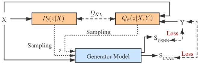
Fig. 4. RGB-D saliency detection via CAVE. The “Generator Model” is shown in Fig. 3. During training, we sample from both posterior net $z\sim$ $Q_{\phi}(z|X,Y)$ and prior net $z\sim P_{\theta}(z|X)$ to obtain predictions $S_{C V A E}$ and $S_{G S N N}$ respectively. During testing, $S_{G S N N}$ is our prediction. 5: end for

图 4: 通过CAVE实现的RGB-D显著性检测。"生成器模型"如图3所示。训练期间，我们分别从后验网络$z\sim Q_{\phi}(z|X,Y)$和先验网络$z\sim P_{\theta}(z|X)$采样，获得预测结果$S_{C V A E}$和$S_{G S N N}$。测试阶段采用$S_{G S N N}$作为预测结果。5: end for

As explained in [23], the conditional auto-encoding of output variables at training may not be optimal to make predictions at test time, as the CVAE uses a posterior of $z$ $(z\sim Q_{\phi}(z|X,Y))$ for the reconstruction loss in the training stage, while it uses the prior of $z$ $(z\sim P_{\theta}(z|X))$ during testing. One solution to mitigate the discrepancy in encoding the latent variable at training and testing is to allocate more weights to the KL loss term (e.g., $\lambda_{k l})$ . Another solution is setting the posterior network the same as the prior network, i.e., $Q_{\phi}(z|X,Y)=P_{\theta}(z|X)$ , and we can sample the latent variable $z$ directly from prior network in both training and testing stages. We call this model the “Gaussian Stochastic Neural Network” (GSNN) [23], and the objective function is:

如[23]所述，训练阶段对输出变量的条件自编码可能无法在测试时实现最优预测，因为CVAE在训练阶段使用后验分布 $z$ $(z\sim Q_{\phi}(z|X,Y))$ 计算重构损失，而在测试时却使用先验分布 $z$ $(z\sim P_{\theta}(z|X))$。缓解训练与测试阶段隐变量编码差异的一种方案是增加KL损失项权重(如 $\lambda_{k l}$)。另一种方案是将后验网络设置为与先验网络相同，即 $Q_{\phi}(z|X,Y)=P_{\theta}(z|X)$，这样在训练和测试阶段都能直接从先验网络采样隐变量 $z$。我们将该模型称为"高斯随机神经网络"(GSNN)[23]，其目标函数为：

$$
\mathcal{L}{\mathrm{GSNN}}=E_{z\sim P_{\theta}(z|X)}[-\log P_{\omega}(Y|X,z)].
$$

We can combine the two objective functions introduced above ( $\mathcal{L}{\mathrm{CVAE}}$ and $\mathcal{L}_{\mathrm{GSNN}}$ to obtain a hybrid objective function:

我们可以将上述两个目标函数 ( $\mathcal{L}{\mathrm{CVAE}}$ 和 $\mathcal{L}_{\mathrm{GSNN}}$ ) 结合起来，得到一个混合目标函数:

$$
{\mathcal{L}}{\mathrm{Hybrid}}=\alpha{\mathcal{L}}{\mathrm{CVAE}}+(1-\alpha){\mathcal{L}}_{\mathrm{GSNN}}
$$

Following the standard practice of CVAE [23], we design a CVAE-based RGB-D saliency detection pipeline as shown in Fig. 4. The two inference models $(Q_{\phi}(z|X,Y)$ and $P_{\theta}(z|X))$ share same structure as shown in Fig. 5, except for $Q_{\phi}(z|X,Y)$ , we have concatenation of $X$ and $Y$ as input, while $P_{\theta}(z|X)$ takes $X$ as input. Let’s define $P_{\theta}(z|X)$ as PriorNet, which maps the input RGB-D data $X$ to a low-dimensional latent feature space, where $\theta$ is the parameter set of PriorNet. With the provided GT saliency map $Y$ , we define $Q_{\phi}(z|X,Y)$ as Posterior Net, with $\phi$ being the network parameter set. We use five convolutional layers and two fully connected layers to map the input RGB-D image $X$ (or concatenation of $X$ and $Y$ for Posterior Net) to the statistics of the latent space: $(\mu_{\mathrm{prior}},\sigma_{\mathrm{prior}})$ for PriorNet and $(\mu_{\mathrm{post}},\sigma_{\mathrm{post}})$ for Posterior Net respectively. Then the corresponding latent vector $z$ can be achieved with the re parameter ation trick: $z=\mu+\sigma\cdot\epsilon$ , where $\epsilon\sim\mathcal{N}(0,{\bf I})$ .

遵循CVAE [23]的标准实践，我们设计了一个基于CVAE的RGB-D显著性检测流程，如图4所示。两个推理模型$(Q_{\phi}(z|X,Y)$和$P_{\theta}(z|X))$共享图5所示的相同结构，不同之处在于$Q_{\phi}(z|X,Y)$以$X$和$Y$的拼接作为输入，而$P_{\theta}(z|X)$仅以$X$为输入。我们将$P_{\theta}(z|X)$定义为PriorNet，它将输入的RGB-D数据$X$映射到低维潜在特征空间，其中$\theta$是PriorNet的参数集。在给定GT显著性图$Y$的情况下，我们将$Q_{\phi}(z|X,Y)$定义为Posterior Net，$\phi$是其网络参数集。我们使用五个卷积层和两个全连接层将输入的RGB-D图像$X$（或Posterior Net中$X$与$Y$的拼接）映射到潜在空间的统计量：PriorNet对应$(\mu_{\mathrm{prior}},\sigma_{\mathrm{prior}})$，Posterior Net对应$(\mu_{\mathrm{post}},\sigma_{\mathrm{post}})$。随后通过重参数化技巧获得对应的潜在向量$z$：$z=\mu+\sigma\cdot\epsilon$，其中$\epsilon\sim\mathcal{N}(0,{\bf I})$。

According to Eq. 4, the KL-divergence in $\mathcal{L}{\mathrm{{CVAE}}}$ is used to measure the distribution mismatch between the $P_{\theta}(z|X)$ and $Q_{\phi}(z|X,Y)$ , or how much information is lost when using $Q_{\phi}(z|X,Y)$ to represent $P_{\theta}(z|X)$ . The GSNN loss term $\mathcal{L}_{\mathrm{GSNN}}$ , on the other hand, can mitigate the discrepancy in encoding the latent variable during training and testing. The hybrid loss in Eq. 4 can achieve structured outputs with hyper-parameter $\alpha$ to balance the two objective functions in Eq. 2 and Eq. 3.

根据式4，$\mathcal{L}{\mathrm{{CVAE}}}$中的KL散度用于衡量$P_{\theta}(z|X)$与$Q_{\phi}(z|X,Y)$之间的分布差异，即用$Q_{\phi}(z|X,Y)$表示$P_{\theta}(z|X)$时会损失多少信息。另一方面，GSNN损失项$\mathcal{L}_{\mathrm{GSNN}}$可以缓解训练和测试时潜在变量编码的差异。式4中的混合损失通过超参数$\alpha$平衡式2和式3中的两个目标函数，从而实现结构化输出。

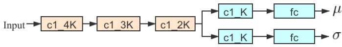
Fig. 5. Detailed structure of inference models, where $K$ is dimension of the latent space, “c1 4K” represents a $1\times1$ convolutional layer of output channel size $4\times K$ , “fc” represents the fully connected layer.

图 5: 推理模型的详细结构，其中 $K$ 表示潜在空间的维度，"c1 4K"代表输出通道大小为 $4\times K$ 的 $1\times1$ 卷积层，"fc"表示全连接层。

Infer $z$ with ABP: As mentioned earlier, one drawback of CVAE-based models is the posterior collapse problem [27], where the model learns to ignore the latent variable, thus it becomes independent of the prediction $Y$ , as $Q_{\phi}(z|X,Y)$ will simply collapse to $P_{\theta}(z|X)$ , and $z$ embeds no information about the prediction. In our scenario, the “Posterior Collapse” phenomenon can be interpreted as the fact that the latent variable $z$ fails to capture the inherent human uncertainty in the annotations. To this end, we propose another alternative solution based on alternating back-propagation [24]. Instead of approximating the posterior of $z$ with an encoder network as in a CVAE, we directly sample $z$ from its true posterior distribution via gradient based MCMC.

使用ABP推断$z$：如前所述，基于CVAE模型的一个缺陷是后验坍塌问题[27]，即模型学会忽略隐变量，导致其与预测$Y$无关。当$Q_{\phi}(z|X,Y)$坍缩为$P_{\theta}(z|X)$时，$z$将不再包含任何预测信息。在我们的场景中，"后验坍塌"现象可解释为隐变量$z$未能捕捉标注中固有的人类不确定性。为此，我们提出另一种基于交替反向传播[24]的解决方案。不同于CVAE中通过编码器网络近似$z$的后验分布，我们直接通过基于梯度的MCMC从其真实后验分布中采样$z$。

Alternating Back-Propagation [24] was introduced for learning the generator network model. It updates the latent variable and network parameters in an EM-manner. Firstly, given network prediction with the current parameter set, it infers the latent variable by Langevin dynamics based MCMC, which they call “Inferential back-propagation” [24]. Secondly, given the updated latent variable, the network parameter set is updated with gradient descent, and they call it “Learning back-propagation” [24]. Following the previous variable definitions, given the training example $(X,Y)$ , we intend to infer $z$ and learn the network parameter $\omega$ to minimize the reconstruction error as well as a regular iz ation term that corresponds to the prior on $z$ .

交替反向传播 [24] 被提出用于学习生成器网络模型。该方法以EM方式更新潜变量和网络参数：首先基于当前参数集进行网络预测，通过朗之万动力学的MCMC方法推断潜变量（称为"推断反向传播" [24]）；其次根据更新后的潜变量，采用梯度下降法更新网络参数集（称为"学习反向传播" [24]）。沿用先前的变量定义，给定训练样本 $(X,Y)$ ，我们需要推断 $z$ 并学习网络参数 $\omega$ ，以最小化重构误差及对应于 $z$ 先验的正则项。

As a non-linear generalization of factor analysis, the conditional generative model aims to generalize the mapping from continuous latent variable $z$ to the prediction $Y$ conditioned on the input image $X$ . As in traditional factor analysis, we define our generative model as:

作为因子分析的非线性推广，条件生成模型旨在泛化从连续潜在变量$z$到预测$Y$的映射，并以输入图像$X$为条件。与传统因子分析类似，我们将生成模型定义为：

$$
\begin{array}{r l}&{z\sim P(z)=\mathcal{N}(0,\mathbf{I}),}\ &{Y=f_{\omega}(X,z)+\epsilon,\epsilon\sim\mathcal{N}(0,\mathrm{diag}(\sigma)^{2}),}\end{array}
$$

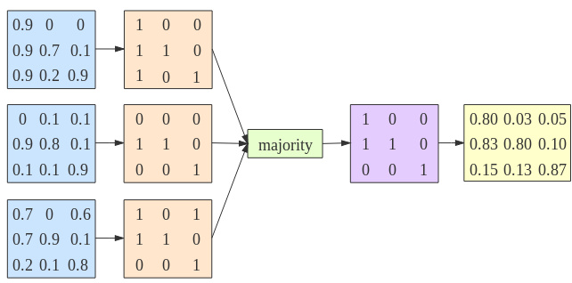
Fig. 6. Example showing how the saliency consensus module works.

图 6: 展示显著性共识模块工作原理的示例。

where $P(z)$ is the prior distribution of $z$ . The conditional distribution of $Y$ given $X$ is $\begin{array}{r}{P_{\omega}(Y|X)=\int p(z)P_{\omega}(Y|X,z)d z}\end{array}$ with the latent variable $z$ integrated out. We define the observed-data loglikelihood as $\begin{array}{r}{L(\omega)\stackrel{{}}{=}\sum_{i=1}^{n}\log P_{\omega}(Y_{i}|X_{i})}\end{array}$ , where the gradient of $P_{\omega}(Y|X)$ is defined as:

其中 $P(z)$ 是 $z$ 的先验分布。给定 $X$ 时 $Y$ 的条件分布为 $\begin{array}{r}{P_{\omega}(Y|X)=\int p(z)P_{\omega}(Y|X,z)d z}\end{array}$，其中隐变量 $z$ 被积分掉。我们将观测数据的对数似然定义为 $\begin{array}{r}{L(\omega)\stackrel{{}}{=}\sum_{i=1}^{n}\log P_{\omega}(Y_{i}|X_{i})}\end{array}$，其中 $P_{\omega}(Y|X)$ 的梯度定义为：

$$
\begin{array}{l}{{\displaystyle\frac{\partial}{\partial\omega}\log P_{\omega}(Y|X)=\frac{1}{P_{\omega}(Y|X)}\frac{\partial}{\partial\omega}P_{\omega}(Y|X)}}\ {{\displaystyle=\mathrm{E}{P_{\omega}(z|X,Y)}\left[\frac{\partial}{\partial\omega}\log P_{\omega}(Y,z|X)\right].}}\end{array}
$$

The expectation term $\operatorname{E}{P_{\omega}(z\vert X,Y)}$ can be approximated by drawing samples from $P_{\omega}(z|X,Y)$ , and then computing the Monte Carlo average. This step corresponds to inferring the latent variable $z$ . Following ABP [24], we use Langevin Dynamics based MCMC (a gradient-based Monte Carlo method) to sample $z$ , which iterates:

期望项 $\operatorname{E}{P_{\omega}(z\vert X,Y)}$ 可通过从 $P_{\omega}(z|X,Y)$ 中抽取样本并用蒙特卡洛平均近似计算。该步骤对应于推断潜变量 $z$。根据 ABP [24] 的方法，我们采用基于朗之万动力学 (Langevin Dynamics) 的 MCMC（一种基于梯度的蒙特卡洛方法）对 $z$ 进行采样，其迭代公式为：

$$
z_{t+1}=z_{t}+\frac{s^{2}}{2}\left[\frac{\partial}{\partial z}\log P_{\omega}(Y,z_{t}|X)\right]+s\mathcal{N}(0,I_{d}),
$$

with

与

$$
\frac{\partial}{\partial z}\log P_{\omega}(Y,z|X)=\frac{1}{\sigma^{2}}(Y-f_{\omega}(X,z))\frac{\partial}{\partial z}f_{\omega}(X,z)-z,
$$

where $t$ is the time step for Langevin sampling, and $s$ is the step size. The whole pipeline of inferring latent variable $z$ via ABP is shown in Algorithm 1.

其中 $t$ 是朗之万采样的时间步长，$s$ 是步长。通过ABP推断潜在变量 $z$ 的完整流程如算法1所示。

Analysis of two inference models: Both the CVAE-based [23] inference model and ABP-based [24] strategy can infer latent variable $z$ , where the former one approximates the posterior distribution of $z$ with an extra encoder, while the latter solution targets at MLE by directly sampling from the true posterior distribution. As mentioned above, the CVAE-based solution may suffer from posterior collapse [27], where the latent variable $z$ is independent of the prediction, making it unable to represent the uncertainty of labeling. To prevent posterior collapse, we adopt the KL annealing strategy [28], [29], and let the KL loss term in Eq. 2 gradually contribute to the CVAE loss function. On the contrary, the ABP-based solution suffers no posterior collapse problem, which leads to simpler and more stable training, where the latent variable $z$ is updated based on the current prediction. In both of our proposed solutions, with the inferred Gaussian random variable $z$ , our model can lead to stochastic prediction, with $z$ representing labeling variants.

两种推断模型分析：基于CVAE [23]的推断模型和基于ABP [24]的策略都能推断潜在变量$z$，前者通过额外编码器近似$z$的后验分布，后者则直接从真实后验分布采样以实现最大似然估计(MLE)。如前所述，基于CVAE的方案可能面临后验坍塌[27]问题，即潜在变量$z$与预测无关，导致其无法表示标注的不确定性。为防止后验坍塌，我们采用KL退火策略[28][29]，使公式2中的KL损失项逐步作用于CVAE损失函数。相反，基于ABP的方案不存在后验坍塌问题，训练过程更简单稳定，其潜在变量$z$会根据当前预测动态更新。在我们提出的两种方案中，通过推断出的高斯随机变量$z$，模型可实现随机预测，其中$z$代表标注变异。

3.3 Output Estimation

3.3 输出估计

Once the generative model parameters are learned, our model can produce prediction from input $X$ following the generative process of the conditional generative model. With multiple iterations of sampling, we can obtain multiple saliency maps from the same input $X$ . To evaluate performance of the generative network, we need to estimate the deterministic prediction of the structured outputs. Inspired by [23], our first solution is to simply average the multiple predictions. Alternatively, we can obtain multiple $z$ from the prior distribution, and define the deterministic prediction as $Y=f_{\omega}(X,E(z))$ , where $E(z)$ is the mean of the multiple latent variable. Inspired by how the GT saliency map is obtained (e.g., Majority Voting), we introduce a third solution, namely “Saliency Consensus Module”, which is introduced in detail.

一旦生成模型的参数被学习，我们的模型就可以按照条件生成模型的生成过程从输入$X$中产生预测。通过多次采样迭代，我们可以从同一输入$X$中获得多个显著性图。为了评估生成网络的性能，我们需要估计结构化输出的确定性预测。受[23]启发，我们的第一种解决方案是简单地对多次预测取平均。另一种方法是从先验分布中获取多个$z$，并将确定性预测定义为$Y=f_{\omega}(X,E(z))$，其中$E(z)$是多个潜变量的均值。受GT显著性图获取方式(如多数投票)的启发，我们引入了第三种解决方案，即"显著性共识模块"，其细节将在后文详述。

Saliency Consensus Module: To prepare a training dataset for saliency detection, multiple annotators are asked to label one image, and the majority [16] of saliency regions is defined as being salient in the final GT saliency map.

显著性共识模块：为准备显著性检测的训练数据集，需让多名标注者对同一图像进行标注，并将多数[16]标注者标记的显著区域定义为最终GT（Ground Truth）显著性图中的显著区域。

Although the way in which the GT is acquired is well known in the saliency detection community yet, there exists no research on embedding this mechanism into deep saliency frameworks. The main reason is that current models define saliency detection as a point estimation problem instead of a distribution estimation problem, and the final single saliency map can not be further processed to achieve “majority voting”. We, instead, design a stochastic learning pipeline to obtain the conditional distributions of prediction, which makes it possible to perform a similar strategy as preparing the training data to generate deterministic prediction for performance evaluation. Thus, we introduce the saliency consensus module to compute the majority of different predictions in the testing stage as shown in Fig. 2 (b).

尽管显著性检测领域对GT（Ground Truth）的获取方式已广为人知，但目前尚未有研究将这一机制嵌入到深度显著性框架中。主要原因是现有模型将显著性检测定义为点估计问题而非分布估计问题，最终生成的单一显著性图无法通过进一步处理实现"多数投票"。为此，我们设计了随机学习流程来获取预测的条件分布，这使得在测试阶段可以采用类似训练数据准备的策略生成确定性预测以进行性能评估。如图2(b)所示，我们通过引入显著性共识模块来计算不同预测结果的多数投票。

During testing, we sample $z$ from PriorNet (for the CVAEbased inference model) or directly sample it from a standard Gaussian distribution ${\mathcal{N}}(0,\mathbf{I})$ , and feed it to the “Generator Model” to produce stochastic saliency prediction as shown in Fig. 2 (b). With $C$ different samplings, we can obtain $C$ predictions $P^{1},...,P^{C}$ . We simultaneously feed these multiple predictions to the saliency consensus module to obtain the consensus of predictions for performance evaluation.

在测试阶段，我们从PriorNet中采样$z$（针对基于CVAE的推理模型）或直接从标准高斯分布${\mathcal{N}}(0,\mathbf{I})$中采样，并将其输入"生成器模型"以产生随机显著性预测，如图2(b)所示。通过$C$次不同采样，可获得$C$组预测结果$P^{1},...,P^{C}$。这些多重预测被同步输入显著性共识模块，以获取预测共识用于性能评估。

Given multiple predictions ${P^{c}}{c=1}^{C}$ , where $P^{c}\in[0,1]$ , we first compute the binary2 version $P_{b}^{c}$ of the predictions by performing adaptive threshold ing [74] on $P^{c}$ . For each pixel $(u,v)$ , we obtain a $C$ dimensional feature vector $P_{u,v}\in{0,1}$ . We define $P_{b}^{m j v}\in{0,1}$ as a one-channel saliency map representing the majority of $P_{u,v}$ , which is defined as:

给定多个预测 ${P^{c}}{c=1}^{C}$ ，其中 $P^{c}\in[0,1]$ ，我们首先通过对 $P^{c}$ 执行自适应阈值化 [74] 来计算预测的二值化版本 $P_{b}^{c}$ 。对于每个像素 $(u,v)$ ，我们得到一个 $C$ 维特征向量 $P_{u,v}\in{0,1}$ 。我们将 $P_{b}^{m j v}\in{0,1}$ 定义为表示 $P_{u,v}$ 多数投票结果的单通道显著性图，其定义为：

$$
P_{b}^{m j v}(u,v)=\left{\begin{array}{l l}{1,}&{\displaystyle\sum_{c=1}^{C}P_{b}^{c}(u,v)/C\geq0.5,}\ {0,}&{\displaystyle\sum_{c=1}^{C}P_{b}^{c}(u,v)/C<0.5.}\end{array}\right.
$$

We define an indicator ${\bf1}^{c}(u,v)={\bf1}(P_{b}^{c}(u,v)=P_{b}^{m j v}(u,v))$ representing whether the binary prediction is consistent with the majority of the predictions. If $P_{b}^{c}(u,v)=P_{b}^{m j v}(u,v)$ , then ${\bf1}^{c}(u,v)=1$ . Otherwise, ${\bf1}^{c}(u,v)~=~0$ . We obtain one gray saliency map after saliency consensus as:

我们定义一个指标 ${\bf1}^{c}(u,v)={\bf1}(P_{b}^{c}(u,v)=P_{b}^{m j v}(u,v))$ 来表示二元预测是否与大多数预测一致。如果 $P_{b}^{c}(u,v)=P_{b}^{m j v}(u,v)$ ，则 ${\bf1}^{c}(u,v)=1$ 。否则， ${\bf1}^{c}(u,v)~=~0$ 。通过显著性共识后，我们得到一个灰度显著性图：

$$
P_{g}^{m j v}(u,v)=\frac{\sum_{c=1}^{C}(P_{b}^{c}(u,v)\times\mathbf{1}^{c}(u,v))}{\sum_{c=1}^{C}\mathbf{1}^{c}(u,v)}.
$$

We show one toy example with $C=3$ in Fig. 6 to illustrate how the saliency consensus module works. As shown in Fig.

我们在图 6 中展示了一个 $C=3$ 的简单示例来说明显著性共识模块的工作原理。如图

As the GT map $Y\in{0,1}$ , we produce a series of binary predictions with each one representing annotation from one saliency annotator.
以GT图 $Y\in{0,1}$ 为基准，我们生成一系列二元预测结果，每个预测代表一位显著性标注者的标注数据。

6, given three gray-scale predictions (illustrated in blue), we perform adaptive threshold ing to obtain three different binary predictions (illustrated in orange). Then we compute a majority matrix (illustrated in purple), which is also binary, with each pixel representing majority prediction of the specific coordinate. Finally, after the saliency consensus module, our final gray-scale prediction is computed based on mean of those pixels agreed (when $P_{b}^{c}(u,v)\stackrel{{}}{=}P_{b}^{m j v}(u,v)$ , we mean in location $u,v$ , the prediction agrees with the majority) with the majority matrix, and ignore others. For example, the majority of saliency in coordinate $(1,1)$ is 1, we obtain the gray prediction after the saliency consensus module as $(0.9+0.7)/2=0.8$ , where 0.9 and 0.7 are predictions in $(1,1)$ of the first and third predictions.

6、给定三个灰度预测（蓝色表示），我们进行自适应阈值处理以获得三个不同的二值预测（橙色表示）。接着计算一个多数矩阵（紫色表示），该矩阵同样为二值形式，每个像素代表对应坐标的多数预测结果。最后通过显著性共识模块，我们仅统计与多数矩阵一致的像素位置（当 $P_{b}^{c}(u,v)\stackrel{{}}{=}P_{b}^{m j v}(u,v)$ 时，表示坐标 $u,v$ 处的预测与多数结果一致），基于这些位置预测值的均值计算最终灰度预测结果，忽略其他位置。例如坐标 $(1,1)$ 的显著性多数结果为1，则显著性共识模块输出的灰度预测值为 $(0.9+0.7)/2=0.8$ ，其中0.9和0.7分别是第一和第三个预测在 $(1,1)$ 位置的预测值。

3.4 Loss function

3.4 损失函数

We introduce two different inference models to update the latent variable $z$ : a CVAE-based model as shown in Fig. 4, and an ABP-based strategy as shown in Algorithm 1. To further highlight structure accuracy of the prediction, we introduce smoothness loss based on the assumption that pixels inside a salient object should have a similar saliency value, and sharp distinction happens along object edges.

我们引入了两种不同的推理模型来更新潜变量 $z$：如图 4 所示的基于 CVAE 的模型，以及如算法 1 所示的基于 ABP 的策略。为了进一步突出预测的结构准确性，我们引入了平滑性损失，其假设是显著物体内部的像素应具有相似的显著值，而显著差异则出现在物体边缘。

As an edge-aware loss, smoothness loss was initially introduced in [75] to encourage disparities to be locally smooth with an L1 penalty on the disparity gradients. It was then adopted in [76] to recover optical flow in the occluded area by using an image prior. We adopt smoothness loss to achieve a saliency map of high intraclass similarity, with consistent saliency prediction inside salient objects, and distinction happens along object edges. Following [76], we define first-order derivatives of the saliency map in the smoothness term as

作为一种边缘感知损失函数，平滑性损失(smoothness loss)最初由[75]提出，通过对视差梯度施加L1惩罚来促使视差局部平滑。随后[76]采用该损失函数，结合图像先验信息来恢复遮挡区域的光流。我们采用平滑性损失来实现具有高类内相似性的显著图，使得显著物体内部预测结果一致，而差异仅出现在物体边缘处。参照[76]的做法，我们在平滑项中将显著图的一阶导数定义为

$$
\mathcal{L}{\mathrm{Smooth}}=\sum_{u,v}\sum_{d\in\overrightarrow{x},\overrightarrow{y}}\Psi(|\partial_{d}P_{u,v}|e^{-\alpha|\partial_{d}I g(u,v)|}),
$$

where $\Psi$ is defined as $\Psi(s)=\sqrt{s^{2}+1e^{-6}}$ , $P_{u,v}$ is the predicted saliency map at position $(u,v)$ , and $I g(u,v)$ is the image intensity, $d$ indexes over partial derivative in $\xrightarrow[{x}]{}$ and $\overrightarrow{y}$ directions. We set $\alpha=10$ in our experiments following the setting in [76].

其中 $\Psi$ 定义为 $\Psi(s)=\sqrt{s^{2}+1e^{-6}}$，$P_{u,v}$ 是位置 $(u,v)$ 处的预测显著图，$I g(u,v)$ 为图像强度，$d$ 表示 $\xrightarrow[{x}]{}$ 和 $\overrightarrow{y}$ 方向上的偏导数索引。实验中我们沿用 [76] 的设置取 $\alpha=10$。

We need to compute intensity $I g$ of the image in the smoothness loss, as shown in Eq. (12). To achieve this, we follow a saliency-preserving [77] color image transformation strategy and convert the RGB image $I$ to a gray-scale intensity image $I g$ as:

我们需要计算平滑损失中图像的强度$I g$，如公式(12)所示。为此，我们采用了一种保留显著性[77]的彩色图像转换策略，将RGB图像$I$转换为灰度强度图像$I g$，具体方法如下：

loss, which integrates the boundary IOU loss [78] to highlight the accuracy of boundary prediction.

损失函数，整合了边界IOU损失 [78] 以突出边界预测的准确性。

With smoothness loss $\mathcal{L}{\mathrm{Smooth}}$ and CVAE loss ${\mathcal{L}}_{{\mathrm{Hybrid}}}$ , our final loss function for the CVAE-based framework is defined as:

在平滑损失 $\mathcal{L}{\mathrm{Smooth}}$ 和 CVAE 损失 ${\mathcal{L}}_{{\mathrm{Hybrid}}}$ 的基础上，我们基于 CVAE 框架的最终损失函数定义为:

$$
{\mathcal{L}}{\mathrm{sal}}^{C V A E}={\mathcal{L}}{\mathrm{Hybrid}}+\lambda_{1}{\mathcal{L}}_{\mathrm{Smooth}}.
$$

We tested $\lambda_{1}$ in the range of $[0.1,0.2,\dots,0.9,1.0]$ , and found ralatively better performance with $\lambda_{1}=0.3$ .

我们测试了 $\lambda_{1}$ 在 $[0.1,0.2,\dots,0.9,1.0]$ 范围内的取值，发现当 $\lambda_{1}=0.3$ 时性能相对较好。

ABP Inference Model based Loss Function: As there exists no extra encoder for the posterior distribution estimation, the loss function for the ABP inference model is simply the negative observed-data log-likelihood:

基于ABP推理模型的损失函数：由于没有额外的编码器用于后验分布估计，ABP推理模型的损失函数仅为观测数据负对数似然：

$$
I g=0.2126\times I^{l r}+0.7152\times I^{l g}+0.0722\times I^{l b},
$$

where $I^{l r},I^{l g}$ , and $I^{l b}$ represent the color components in the linear color space after Gamma function be removed from the original color space. $I^{l r}$ is achieved via:

其中 $I^{l r},I^{l g}$ 和 $I^{l b}$ 表示从原始色彩空间经Gamma函数去除后在线性色彩空间中的颜色分量。$I^{l r}$ 通过以下方式获得：

$$
I^{l r}=\left{\begin{array}{r}{{I^{r}}}\ {{\overline{{{12.92}}},}}\end{array}\right.I^{r}\leq0.04045,
$$

$$
\mathcal{L}{A B P}=-\sum_{i=1}^{n}\log P_{\omega}(Y_{i}|X_{i}),
$$

which can be the same structure-aware loss as in [7] similar to CVAE-based inference model.

可以采用与[7]中相同的结构感知损失（structure-aware loss），类似于基于CVAE的推理模型。

CVAE Inference Model based Loss Function: For the CVAEbased inference model, we show its loss function in Eq. 4, where the negative log-likelihood loss measures the reconstruction error. To preserve structure information and penalize wrong predictions along object boundaries, we adopt the structure-aware loss in [7]. The structure-aware loss is a weighted extension of cross-entropy

基于CVAE推理模型的损失函数：对于基于CVAE的推理模型，我们在公式4中展示了其损失函数，其中负对数似然损失用于衡量重构误差。为保留结构信息并惩罚物体边界处的错误预测，我们采用[7]提出的结构感知损失。该结构感知损失是交叉熵的加权扩展形式

Integrated with the above smoothness loss, we obtain the loss function for the ABP-based saliency detection model as:

结合上述平滑度损失，我们得到基于ABP的显著性检测模型的损失函数为：

where $I^{r}$ is the original red channel of image $I$ , and we compute $I^{g}$ and $I^{b}$ in the same way as Eq. (14).

其中 $I^{r}$ 是图像 $I$ 的原始红色通道，我们按照式 (14) 相同的方式计算 $I^{g}$ 和 $I^{b}$。

$$
\begin{array}{r}{\mathcal{L}{\mathrm{sal}}^{A B P}=\mathcal{L}{A B P}+\lambda_{2}\mathcal{L}_{\mathrm{Smooth}}.}\end{array}
$$

Similarly, we also empirically set $\lambda_{2}=0.3$ in our experiment.

同样地，我们在实验中也经验性地设定 $\lambda_{2}=0.3$。

4 EXPERIMENTAL RESULTS

4 实验结果

4.1Setup

4.1 设置

Datasets: We perform experiments on six datasets including five widely used RGB-D saliency detection datasets (namely NJU2K [85], NLPR [80], SSB [90], LFSD [91], DES [82]) and one newly released dataset (SIP [16]).

数据集：我们在六个数据集上进行了实验，包括五个广泛使用的RGB-D显著性检测数据集（即NJU2K [85]、NLPR [80]、SSB [90]、LFSD [91]、DES [82]）和一个新发布的数据集（SIP [16]）。

Competing Methods: We compare our method with 18 algorithms, including ten handcrafted conventional methods and eight deep RGB-D saliency detection models.

竞争方法：我们将所提方法与18种算法进行比较，包括10种手工设计的传统方法和8种基于深度学习的RGB-D显著性检测模型。

Evaluation Metrics: Four evaluation metrics are used to evaluate the deterministic predictions, including two widely used: 1) Mean Absolute Error (MAE $\mathcal{M}{{}}$ ); 2) mean F-measure $(F_{\beta})$ and two recently proposed: 3) Structure measure (S-measure, $S_{\alpha}$ ) [98] and 4) mean Enhanced alignment measure (E-measure, $E_{\xi}$ ) [79].

评估指标：采用四种评估指标来衡量确定性预测结果，包括两种广泛使用的指标：1) 平均绝对误差 (MAE $\mathcal{M}{{}}$ )；2) 平均F值 $(F_{\beta})$ ，以及两种近年提出的指标：3) 结构度量 (S-measure, $S_{\alpha}$ ) [98] 和 4) 平均增强对齐度量 (E-measure, $E_{\xi}$ ) [79]。

MAE $\mathcal{M}$ : The MAE estimates the approximation degree between the saliency map $S a l$ and the ground-truth $G$ . It provides a direct estimate of conformity between estimated and GT map. MAE is defined as:

MAE $\mathcal{M}$: MAE用于评估显著性图 $Sal$ 与真实值 $G$ 之间的近似程度。它直接衡量估计图与真实图的吻合度，其定义为:

$$
\mathrm{{MAE}}=\frac{1}{N}|S a l-G|,
$$

where $N$ is the total number of pixels.

其中 $N$ 为像素总数。

S-measure $S_{\alpha}$ : Both MAE and $\mathrm{F}\mathrm{.}$ -measure metrics ignore the important structure information evaluation, whereas behavioral vision studies have shown that the human visual system is highly sensitive to structures in scenes [98]. Thus, we additionally include the structure measure (Smeasure [98]). The S-measure combines the region-aware $(S_{r})$ and object-aware $(S_{o})$ structural similarity as their final structure metric:

S-measure $S_{\alpha}$：MAE和$\mathrm{F}\mathrm{.}$-measure指标均忽略了重要的结构信息评估，而行为视觉研究表明人类视觉系统对场景中的结构高度敏感[98]。因此，我们额外引入了结构度量(Smeasure [98])。S-measure将区域感知$(S_{r})$和对象感知$(S_{o})$的结构相似性结合作为最终结构度量：

$$
S_{\alpha}=\alpha*S_{o}+(1-\alpha)*S_{r},
$$

where $\alpha\in[0,1]$ is a balance parameter and set to 0.5 as default.

其中 $\alpha\in[0,1]$ 是平衡参数，默认设置为 0.5。

E-measure $E_{\xi}$ : E-measure is the recent proposed Enhanced alignment measure [79] in the binary map evaluation field. This measure is based on cognitive vision studies, which combines local pixel values with the imagelevel mean value in one term, jointly capturing image-level statistics and local pixel matching information. Here, we introduce it to provide a more comprehensive evaluation. F-measure $F_{\beta}$ : It is essentially a region based similarity metric. We provide the mean F-measure using varying 255 fixed (0-255) thresholds as shown in Fig. 7.

E-measure $E_{\xi}$：E-measure是二值图评估领域最新提出的增强对齐度量(Enhanced alignment measure) [79]。该度量基于认知视觉研究，将局部像素值与图像级均值结合在一个项中，同时捕获图像级统计信息和局部像素匹配信息。我们引入该指标以提供更全面的评估。
F-measure $F_{\beta}$：本质上是基于区域的相似性度量。如图7所示，我们使用0-255范围内255个固定阈值计算平均F-measure值。

TABLE 1 Benchmarking results of ten leading handcrafted feature-based models and eight deep models on six RGBD saliency datasets. ↑ & ↓ denote larger and smaller is better, respectively. Here, we adopt mean $F_{\beta}$ and mean $E_{\xi}$ [79]. Evaluation tool: https://github.com/Deng Ping Fan/D 3 Net Benchmark.

表 1: 十种领先的基于手工特征的模型和八种深度模型在六个RGBD显著性数据集上的基准测试结果。↑ 和 ↓ 分别表示数值越大越好和越小越好。这里我们采用平均 $F_{\beta}$ 和平均 $E_{\xi}$ [79]。评估工具: https://github.com/Deng Ping Fan/D 3 Net Benchmark。

	Metric	HandcraftedFeaturebasedModels									DeepModels							Ours
		LHM	CDB [81]	DESM [82]	GP [83]	CDCP [84]	ACSD [85]	LBE [86]	DCMC [87]	MDSF [88][89]	SE DF	AFNet [34]	CTMF [18]	MMCI [37]	PCF TANet [36][17]	CPFP	DMRA [10]	UC-NetCVAE ABP [1]
NJU2K [85]	Sα	.514	.632	.665	.527	.669	.699	.695	.686	.748	.664	.763	.822	.849	.858	.877	.879	.878
	FB	.328	.498	.550	.357	.595	.512	.606		.628	.583 .653	.827	.779	.793	.840	.841	.850	.873
	E	.447	.572	.590	.466	.706	.594	.655	.556 .619	.677	.624							.920
	M	.205	.199	.283	.211	.180	.202	.153	.172	.157	.700 .169 .140	.867 .077	.846 .085	.851 .079	.895 .059	.895 .061	.910 .053	.051
	Sα	.562	.615	.642	.588	.713	.692	.660 .731	.728	.708	.757	.825	.848	.873	.875	.871	.879	.835
	↑	.378	.489	.519				.590	.527	.611	.617			.813	.818		.841	.837
	Fβ				.405	.638	.478	.501				.806	.758			.828
	Ee M	.484 .172	.561 .166	.579 .295	.508 .182	.751 .149	.592 .200	.601 .655 .250 .148	.176	.614 .664 .143	.692 .141	.872 .075	.841 .086	.873 .068	.887 .064	.893 .060	.911 .051	.879 .066
DES [82]	Sα FB	.578	.645	.622	.636	.709	.728	.703 .707	.741	.741	.752	.770	.863	.848	.842	.858	.872	.900
		.345	.502	.483	.412	.585	.513	.576 .542	.523	.618	.604	.713	.756	.735	.765	.790	.824	.873
		.477	.572	.566			.613	.650 .631	.621	.706	.684	.809	.826	.825	.838	.863	.888	.933
	E M	.114	.100	.299	.503 .168	.748 .115	.169	.208 .111	.122	.090	.093	.068	.055	.065	.049	.046	.038	.030
NLPR [80]	Sα	.630	.632	.572	.655	.727	.673	.762 .724	.805	.756	.806	.799	.860	.856	.874	.886	.888	.899
		.427	.421	.430	.451	.609	.429	.636	.649	.624	.664			.737	.802		.840	.865
	FB	.560	.567	.542			.579	.542 .684	.745	.742	.757	.755	.740	.841	.887	.819		.940
	Ee M	.108	.108	.312	.571 .146	.782 .112	.179	.719 .081 .117	.095	.091	.079	.851 .058	.840 .056	.059	.044	.902 .041	.918 .036	.031
LFSD[91]	Sα	.557	.520	.722	.640	.717	.734	.736 .753	.700	.698	.791	.738	.796	.787	.794	.801	.828	.847
		.396	.376	.612	.519	.680	.566	.612 .655	.521	.640	.679		.756	.722	.761	.771	.811	.845
	FB E	.491	.465	.638	.584	.754	.625	.670 .682	.588	.653	.725	.736 .796	.810	.775	.818

Fig. 7. E-measure and F-measure curves on six testing datasets (NJU2K, SSB, DES, NLPR, LFSD and SIP). Best viewed on screen.

图 7: 六个测试数据集 (NJU2K、SSB、DES、NLPR、LFSD 和 SIP) 上的 E-measure 和 F-measure 曲线。建议屏幕观看最佳效果。

TABLE 2 The code type and inference time of existing approaches. $\mathsf{M}=$ Matlab. $\mathsf{P t}=\mathsf{P y}$ Torch. Tf $=$ Tensorflow.

表 2: 现有方法的代码类型和推理时间。$\mathsf{M}=$ Matlab。$\mathsf{P t}=\mathsf{P y}$ Torch。Tf $=$ Tensorflow。

方法	LHM [80]	CDB [81]	DESM [82]	GP[83]	CDCP [84]	ACSD[92]	LBE [86]	DCMC [87]	MDSF[88]
时间 (秒)	2.13	0.60	7.79	12.98	60.00	0.72	3.11	1.20	60.00
代码类型	M	M	M	M&C++	M&C++	++	M&C++	M	++
方法	SE [89]	DF [34]	AFNet [35]	CTMF [18]	MMCI [37]	PCF [36]	CPFP [11]	Our_ABP	Our_CVAE
时间 (秒)	1.57	10.36	0.03	0.63	0.05	0.06	0.17	0.05	0.06
代码类型	M&C++	M&C++	Tf	Caffe	Caffe	Caffe	Caffe	Pt	Pt

Fig. 8. Visual comparison of predictions of our methods and competing methods. Note that, our final prediction is generated with the proposed “Saliency Consencus Module” (see Section 3.3).

图 8: 我们的方法与竞争方法预测结果的视觉对比。请注意，我们的最终预测是通过提出的"显著性共识模块"(见第3.3节)生成的。

Implementation Details: We train our model using PyTorch, and initialized the encoder of the “Generator Model” with ResNet50 [73] parameters pre-trained on ImageNet. Inside the “DASPP” module of the “Generator Model” in Fig. 3, we use four different scales of dilation rate: 6, 12, 18, 24 same as [71], and set all intermediate channel size as $M=32$ . For both inference models, we set the dimension of the latent variable as $K=3$ . Weights of new layers are initialized with $\mathcal{N}(0,0.01)$ , and bias is set as constant. We use the Adam method with momentum 0.9 and decrease the learning rate $10%$ after $80%$ of the maximum epoch. The base learning rate is initialized as 5e-5. The whole training takes around 9 hours with training batch size 5, and maximum epoch 100 on a PC with an NVIDIA GeForce RTX GPU. For input image size $352\times352$ , the inference time of our CVAE model and ABP model are 0.06s and 0.05s on average respectively.

实现细节：我们使用PyTorch训练模型，并用在ImageNet上预训练的ResNet50 [73]参数初始化"生成器模型"的编码器。在图3的"生成器模型"的"DASPP"模块中，我们采用与[71]相同的四种不同膨胀率尺度：6、12、18、24，并将所有中间通道尺寸设为$M=32$。对于两个推断模型，我们将潜变量维度设为$K=3$。新层权重采用$\mathcal{N}(0,0.01)$初始化，偏置设为常数。使用动量0.9的Adam方法，并在达到最大训练周期80%后降低学习率10%。基础学习率初始化为5e-5。在配备NVIDIA GeForce RTX GPU的PC上，整个训练耗时约9小时（训练批量大小为5，最大周期100）。对于$352\times352$的输入图像尺寸，我们的CVAE模型和ABP模型平均推断时间分别为0.06秒和0.05秒。

4.2 Comparison to State-of-the-art Methods

4.2 与前沿方法的对比

Quantitative Comparison: We report the performance of our method (with both inference models) and competing methods in Table 1, where “CVAE” is our framework with CVAE as inference model, and “ABP” represents the model that updates latent variable $z$ with alternating back-propagation. Results in Table 1 demonstrate the benefits of both CVAE and ABP which consistently achieve the best performance on all datasets. Specifically, on SSB [90] and SIP [16], our method achieves around a $2.5%$

定量对比：我们在表1中报告了本方法（含两种推理模型）与对比方法的性能表现，其中"CVAE"表示采用CVAE作为推理模型的框架，"ABP"代表通过交替反向传播更新潜在变量$z$的模型。表1结果显示，CVAE和ABP在所有数据集上均保持最佳性能优势。具体而言，在SSB [90]和SIP [16]数据集上，本方法实现了约$2.5%$的性能提升。

S-measure, E-measure and F-measure performance boost and a decrease in MAE by $1.5%$ compared with the “Deep Models” in Table 1. Moreover, compared with our preliminary version “UCNet” [1], we observe improved performance, which indicates the effectiveness of the proposed structure. We also show E-measure and F-measure curves of competing methods and ours in Fig. 7. We observe that our method produces not only stable E-measure and F-measure but also the best performance.

与表1中的"Deep Models"相比，S-measure、E-measure和F-measure性能提升，MAE降低1.5%。此外，与我们的初版"UCNet"[1]相比，我们观察到性能有所改进，这表明所提出结构的有效性。图7展示了竞争方法和我们方法的E-measure和F-measure曲线，可见我们的方法不仅产生稳定的E-measure和F-measure，还实现了最佳性能。

To further evaluate the proposed method, we compute performance of eight cutting-edge RGB saliency detection models on the RGBD testing dataset3 and compared with our “CVAE” based model. The results are shown in Table 3, which further illustrates the superior performance of the proposed framework.

为进一步评估所提出的方法，我们计算了八种前沿RGB显著性检测模型在RGBD测试数据集3上的性能，并与基于"CVAE"的模型进行了对比。结果如表3所示，进一步证明了该框架的优越性能。

Qualitative Comparisons: In Fig. 8, we show five examples comparing our method with six RGB-D saliency detection models. Salient objects in these images can be large (fifth row), small (second row) or in complex backgrounds (first, third, fourth and fifth rows). Especially for the example in the first row, the background is complex, part of the background shares similar color and texture as the salient foreground. Most of those competing methods (AFNet [35], CPFP [11] and DMRA [10]) failed to correctly segment the precise salient foreground, while our approach achieves better salient object detection with each of the proposed two inference models. For the image in the last row, there exists an object (i.e., green toy) that strongly stands out from its background, while the depth map can to some extent decrease the salience of such high-contrast region. All of the competing methods (DCMC [87], SE [89], AFNet [35], CPFP [11] in particular) falsely detect part of the background region as being salient, whereas our accurate predictions further indicate the effectiveness of our solutions. With all the results in Fig. 8, we can see evidence of the superiority of our approach.

定性比较：在图 8 中，我们展示了五个示例，将我们的方法与六种 RGB-D 显著性检测模型进行比较。这些图像中的显著对象可能较大(第五行)、较小(第二行)或处于复杂背景中(第一、三、四、五行)。特别是第一行的示例，背景复杂，部分背景与显著前景具有相似的颜色和纹理。大多数竞争方法(AFNet [35]、CPFP [11] 和 DMRA [10])未能正确分割精确的显著前景，而我们的方法通过提出的两种推理模型均实现了更好的显著对象检测。对于最后一行的图像，存在一个与背景形成强烈对比的对象(即绿色玩具)，而深度图在一定程度上会降低这种高对比度区域的显著性。所有竞争方法(尤其是 DCMC [87]、SE [89]、AFNet [35]、CPFP [11])都错误地将部分背景区域检测为显著区域，而我们的准确预测进一步证明了我们解决方案的有效性。根据图 8 中的所有结果，我们可以看出我们方法的优越性。

TABLE 3 Performance of competing RGB saliency detection models and ours on RGBD saliency datasets, where depth data is not used while testing using the RGB saliency models. We adopt mean $F_{\beta}$ and mean $E_{\xi}$ .

表 3: 竞争性RGB显著性检测模型与我们的模型在RGBD显著性数据集上的性能表现，其中测试时未使用深度数据。我们采用平均 $F_{\beta}$ 和平均 $E_{\xi}$ 作为评估指标。

| | | 指标 | AFBNet [93] | NLDF [78] | PiCANet [94] | RAS [95] | DGRL [96] | CPD [97] | SCRN [9] | F3Net [7] | CAVE Ours |
|---|---|---|---|---|---|---|---|---|---|---|
| NJU2K [92] | Sα↑ | .862 | .813 | .864 | .754 | .767 | .875 | .879 | .861 | .902 |
| | Fβ↑ | .835 | .783 | .818 | .744 | .716 | .852 | .863 | .837 | .893 |
| | Eξ↑ | .888 | .848 | .869 | .800 | .804 | .903 | .912 | .890 | .937 |
| | M↓ | .064 | .091 | .072 | .115 | .107 | .056 | .052 | .061 | .039 |
| SSB [90] | Sα↑ | .893 | .859 | .896 | .828 | .824 | .902 | .902 | .891 | .898 |
| | Fβ↑ | .865 | .831 | .844 | .820 | .781 | .880 | .881 | .868 | .878 |
| | Eξ↑ | .918 | .893 | .899 | .871 | .865 | .928 | .928 | .921 | .935 |
| | M↓ | .045 | .062 | .053 | .076 | .073 | .040 | .041 | .043 | .039 |
| DES [82] | Sα↑ | .879 | .828 | .883 | .806 | .833 | .894 | .907 | .880 | .937 |
| | Fβ↑ | .845 | .758 | .822 | .762 | .753 | .870 | .885 | .845 | .929 |
| | Eξ↑ | .893 | .831 | .872 | .823 | .849 | .907 | .927 | .892 | .975 |
| | M↓ | .035 | .058 | .039 | .060 | .054 | .029 | .026 | .030 | .016 |
| NLPR [80] | Sα↑ | .881 | .847 | .876 | .853 | .840 | .893 | .894 | .884 | .917 |
| | Fβ↑ | .816 | .782 | .789 | .810 | .767 | .844 | .846 | .838 | .893 |
| | Eξ↑ | .896 | .876 | .870 | .888 | .873 | .914 | .920 | .912 | .952 |
| | M↓ | .042 | .052 | .051 | .049 | .053 | .034 | .036 | .035 | .025 |
| LFSD [91] | Sα↑ | .817 | .777 | .827 | .673 | .782 | .836 | .827 | .835 | .868 |
| | Fβ↑ | .784 | .756 | .778 | .672 | .759 | .811 | .800 | .810 | .857 |
| | Eξ↑ | .838 | .806 | .825 | .727 | .817 | .856 | .847 | .857 | .904 |
| | M↓ | .094 | .121 | .103 | .162 | .117 | .088 | .088 | .089 | .065 |
| SIP [16] | Sα↑ | .876 | .795 | .851 | .718 | .682 | .870 | .866 | .866 | .883 |
| | Fβ↑ | .847 | .752 | .806 | .696 | .606 | .859 | .861 | .850 | .877 |
| | Eξ↑ | .911 | .840 | .866 | .766 | .744 | .910 | .903 | .905 | .927 |
| | M↓ | .055 | .100 | .073 | .121 | .138 | .053 | .057 | .055 | .045 |

Probabilistic Distribution Evaluation: As a probabilistic network, our models can produce a distribution of plausible saliency maps instead of a single, deterministic prediction for each input image. We argue that, for images with simple background, consistent predictions should be produced, whereas for complex images with cluttered background, we expect our model to capture the uncertainty in the saliency maps, and thus can generate diverse predictions. To evaluate performance of our model, following the active learning pipeline [99], we first generate $B=100$ easy and difficult samples. To achieve this, we first adopt three different conventional saliency models (RBD [100], MR [101] and GS [102], which rank among the top six conventional handcrafted feature based RGB saliency models [74]), and define them as $f1,f2$ and $f3$ respectively. Given image $X_{i}^{4}$ in training dataset $D$ , we compute its corresponding saliency map $f1(X_{i})$ , $f2(X_{i})$ and $f3(X_{i})$ . We choose entropy as measure for image complexity. Then, we define mean saliency map of $X_{i}$ as $P_{i}=(f1(X_{i})+f2(X_{i})+f3(X_{i}))/3$ . We define the complexity of the image as task driven (for saliency detection). Then given a ground-truth saliency map $Y_{i}$ and mean saliency map $P_{i}$ , we define foreground entropy as: $-P_{i}\log P_{i}$ .

概率分布评估：作为一种概率网络，我们的模型能够为每张输入图像生成一组可能的显著图分布，而非单一确定性预测。我们认为，对于背景简单的图像，模型应产生一致的预测；而对于背景杂乱的复杂图像，模型需要捕捉显著图中的不确定性，从而生成多样化预测。为评估模型性能，我们遵循主动学习流程[99]，首先生成$B=100$个简单和困难样本。具体实现时，采用三种传统显著模型（RBD[100]、MR[101]和GS[102]，这些模型位列基于手工特征的RGB显著模型前六名[74]），分别定义为$f1,f2$和$f3$。给定训练集$D$中的图像$X_{i}^{4}$，计算其对应显著图$f1(X_{i})$、$f2(X_{i})$和$f3(X_{i})$。选择熵作为图像复杂度度量指标，将$X_{i}$的平均显著图定义为$P_{i}=(f1(X_{i})+f2(X_{i})+f3(X_{i}))/3$。图像复杂度定义为任务驱动型（针对显著检测）。给定真实显著图$Y_{i}$和平均显著图$P_{i}$时，前景熵定义为：$-P_{i}\log P_{i}$。

We then define mean entropy as a complexity measure, and choose $B$ images with the smallest entropy as the easy samples and $B$ images with the largest entropy as the difficult samples (with $B=100;$ ). We sample $S n~=~5$ times from the prior distribution and compute the variance of each group. Specifically, for image pair $X_{i}$ , with $S n$ iterations of sampling, we obtain its prediction ${S_{i}^{j}}_{j=1}^{S n}$ . We compute the similarity of these $S n$ different predictions, and treat it as prediction diversity evaluation. We show entropy and standard deviation of images in Fig. 10.

我们定义平均熵(entropy)作为复杂度度量指标，选取熵值最小的$B$张图像作为简单样本，熵值最大的$B$张图像作为困难样本(设定$B=100$)。我们从先验分布中采样$S n~=~5$次并计算每组方差。具体而言，对于图像对$X_{i}$，经过$S n$次采样迭代后获得其预测结果${S_{i}^{j}}_{j=1}^{S n}$。我们计算这$S n$个不同预测结果的相似度，并将其作为预测多样性评估指标。图10展示了图像的熵值和标准差分布。

Inference $\mathbf{Time^{5}}$ Comparison: We summarize basic information of competing methods in Table 2 for clear comparison, including their code type and inference time. Table 2 shows that the inference time6 of our method is comparable with competing methods, which further illustrates that our model can achieve probabilistic predictions with no inference time sacrificed.

推理时间$\mathbf{Time^{5}}$对比：我们在表2中总结了竞争方法的基本信息以便清晰比较，包括其代码类型和推理时间。表2显示，我们方法的推理时间6与竞争方法相当，这进一步说明我们的模型能在不牺牲推理时间的情况下实现概率预测。

4.3 Structured Output Generation

4.3 结构化输出生成

As a generative network, we introduce a latent variable $z$ modeling uncertainty of human annotation. We further show examples of our model generating structured outputs as shown in Fig. 9. The “Our CVAE Samples” in Fig. 9 represents three random samples of our method with the CVAE inference model, and “Our ABP Samples” are samples with the ABP strategy. “Our CVAE” and “Our ABP” are the deterministic predictions of our frameworks with the above two inference models obtained via our “Saliency Consensus Module”. Fig. 9 shows that both the two inference models can produce reasonable stochastic predictions, and the final deterministic prediction after the “Saliency Consensus Module” (“Our CVAE” and “Our ABP”) is consistent with the provided GT, which verifies effectiveness of both our latent variable and the “Saliency Consensus Module”.

作为生成网络，我们引入了一个潜在变量$z$来建模人工标注的不确定性。图9展示了我们的模型生成结构化输出的示例。其中"我们的CVAE样本"代表使用CVAE推理模型随机生成的三组结果，"我们的ABP样本"则是采用ABP策略生成的样本。"我们的CVAE"和"我们的ABP"分别表示通过"显著性共识模块"获取的两种推理框架的确定性预测结果。图9表明，两种推理模型都能产生合理的随机预测，且经过"显著性共识模块"处理后的最终确定性预测结果（"我们的CVAE"和"我们的ABP"）与给定的GT保持一致，这验证了我们提出的潜在变量和"显著性共识模块"的有效性。

4.4 Ablation Studies

4.4 消融实验

We further analyse the proposed framework in this section, including the generative network related strategies, the loss functions, the alternative depth data (HHA [103] in particular), and the solution to prevent network from posterior collapse. We show the performance in Table 4. Note that unless otherwise stated, we use the CVAE-based inference model in the following experiments.

本节将进一步分析所提出的框架，包括生成网络相关策略、损失函数、替代深度数据（特别是HHA [103]），以及防止网络后验坍塌的解决方案。性能展示如表4所示。请注意，除非另有说明，后续实验均采用基于CVAE的推理模型。

Different Fusion Schemes: The latent variable $z$ can be fused to the network in three different ways: early fusion (in the input layer), middle fusion (in bottleneck network), or late fusion (before the output layer). We propose an early fusion model as shown in Fig. 11 (a). We further design a middle fusion models and a late fusion model as shown in Fig. 11 (b) and (c) respectively. The performance of each model is shown in Table 4 “Middle” and “Late”. For the middle fusion model, last convolutional layer of the fourth group (e.g., S4) of the backbone network is fed to a $1\times1$ convolutional layer to obtain a $M=32$ dimensional feature map, which is then map to a $K$ (dimension of the latent variable $z$ ) dimensional feature vector with a fully connected layer (“fc”). To avoid posterior collapse [27], inspired by [52], we mix (“Mixup”) the feature vector and $z$ channel-wise; thus, the network cannot distinguish between features of the deterministic branch and the probabilistic branch. We then expand the mixed feature vector in the spatial dimension, and feed it to another $1\times1$ convolutional layer to achieve feature map $\mathbf{S4}^{\star}$ of the same dimension as S4, and replace S4 with $\mathbf{S4}^{,}$ in Fig. 3. For the late fusion model, the “Generator Model” represents the generator model in Fig. 3 before the last “RCA” module. We expand $z$ in spatial dimension and concatenate it with the deterministic feature. We also perform “Mixup” here similar to the middle fusion model. We then feed the mixed feature map to one “RCA” module and “DASPP” model to achieve prediction $S$ . We observe slightly worse performance of the middle fusion model (“Middle”) and late fusion model (“Late”). The main reason is that strong non-linear representation can be obtained when the latent variable is fed to the beginning of the network, which is also consistent with the result that “Middle” is better than “Late”.

不同融合方案：潜在变量$z$可通过三种方式融入网络：早期融合（输入层）、中期融合（瓶颈网络）或晚期融合（输出层前）。如图11(a)所示，我们提出早期融合模型，并分别设计了图11(b)和(c)的中期与晚期融合模型。各模型性能见表4"Middle"和"Late"。对于中期融合模型，主干网络第四组（如S4）的末层卷积经$1×1$卷积层生成$M=32$维特征图，再通过全连接层("fc")映射为$K$（潜在变量$z$的维度）维特征向量。为避免后验坍塌[27]，受[52]启发，我们对特征向量和$z$进行通道混合("Mixup")，使网络无法区分确定性分支和概率性分支的特征。随后将混合向量空间维度扩展，输入另一个$1×1$卷积层生成与S4同维的特征图$\mathbf{S4}^{\star}$，并在图3中用$\mathbf{S4}^{,}$替换S4。晚期融合模型中，"Generator Model"对应图3末个"RCA"模块前的生成器模型。我们将$z$空间扩展后与确定性特征拼接，并执行类似中期融合的"Mixup"操作，混合特征图经"RCA"模块和"DASPP"模型得到预测$S$。实验表明中期("Middle")和晚期("Late")融合模型性能略逊，主因是潜在变量在网络起始端输入能获得更强非线性表征，这也与"Middle"优于"Late"的结果一致。

TABLE 4 Evaluation of the effect of different components in our models, and alternative structures. We present mean $F_{\beta}$ and mean $E_{\xi}$

表 4: 模型不同组件及替代结构的评估结果，展示平均 $F_{\beta}$ 和平均 $E_{\xi}$

Method	NJU2K	SSB	DES	NLPR	LFSD	SIP
Middle	.897 .888 .933 .042	.895 5.880 .934 .041	.931 .920 .968 .018	.916 .887 .950 .026	.854 .843 .888 .073	.873 .863 .914 .048
Late	.890 .875 .929 .046	.891 .866 5.931 .042	.929 .909 .970 .020	.907 .877 .947 .028	.839 .828 .887 .076	.870 .853 .916 .051
AveP	.900 .892 .936 .040	.897 .877 .934 .040	.935 .924 .970 .017	.914 .890 .951 .025	.857 .842 .899 .067	.880 .876 .926 .046
AveZ	.901 .890 .927 .040	.892 .875 .930 .040	.929 .921 .971 .018	.914 .884 .950 .026	.855 .843 .892 .068	.880 .874 .926 .046
GSNN	.900 .887 .935 .040	.894 .873 .930 .041	.931 .919 .971 .018	.913 .885 .949 .026	.852 .834 .894 .070	.871 .864 .916 .051
CVAE_S	.900 .890 .932 .040	.894 .876 5.931 .041	.936 .927 .974 .016	.914 4.891 .949 .026	.856 .843 .897 .068	.877 .867 .920 .048
NoS	.893 .881 .933 .042	.885 .876 5.930 .044	.931 .921 .966 .017	914 .878 .950 .027	853 .845 .898 .069	.882 .868 .924 .047
CE	.900 .891 .936 .041	.894 .876 5.930 .040	.935 .921 .970 .018	.913 .891 .950 .025	.851 .833 .887 .075	.876 .856 .916 .051
HHA	.897 .886 .934 .042	.902 .882 .937 .038	.930 .917 .970 .019	.919 .892 .950 .024	.850 .834 .888 .074	.870 .856 .915 .052
w/oKLA	.900 .890 .932 .041	.893 .870 .931 .040	.932 .923 .972 .017	.913 .887 .948 .027	.854 .841 .893 .069	.881 .872 .923 .046
Our_CAVE	.902 .893 .937 .039	.898 .878 .935 .039	.937 .929 .975 .016	.917 .893 .952 .025	.868 .857 .904 .065	.883 .877 .927 .045
Our_ABP	.900 .889 .937 .039	.904 4.886 .939 .037	.940 .928 .975 .016	.919 .891 .852 .024	.866 .859 .903 .065	.876 .863 .921 .049

Fig. 9. Structured outputs generation, where “Our CVAE Samples” and “Our CVAE” are samples and the deterministic prediction respectively.

图 9: 结构化输出生成示例，其中"Our CVAE Samples"和"Our CVAE"分别表示采样结果和确定性预测。

Fig. 10. Image distribution by analysing entropy and standard deviation.

图 10: 通过分析熵和标准差得到的图像分布。

Analysing the Effect of the Dimension of $z$ : The scale of $z$ may influence both network performance and diversity of predictions. In this paper, we set dimension of $z$ to 3. We further carry out experiments with dimension of $z$ in the range of [3, 32], and show mean absolution error of our model on six benchmark RGB-D saliency dataset in Fig. 12. We observe relatively stable performance for different dimension of $z$ . The relatively stable performance regardless of dimension of $z$ shows that the capacity of the network is large enough to take different degree of stochasticity in the input. Meanwhile, as there exists only a few quite difficult samples, and lower dimension of $z$ is enough to capture variants of labeling.

分析 $z$ 维度的影响：$z$ 的尺度可能影响网络性能和预测多样性。本文设定 $z$ 的维度为3，并进一步在[3, 32]范围内进行实验。如图12所示，我们在六个RGB-D显著性基准数据集上展示了模型在不同 $z$ 维度下的平均绝对误差。实验观察到不同 $z$ 维度下性能相对稳定，这表明网络容量足以处理输入中不同程度随机性。同时由于困难样本较少，较低维度的 $z$ 已能充分捕捉标注变体。

Deterministic Prediction Generation: As introduced in Section 3.3, three different solutions can be used to generate a deterministic prediction for performance evaluation, including 1) averaging multiple predictions; 2) averaging multiple latent variables; and 3) the proposed saliency consensus module. We evaluate performance of other deterministic inference solutions and show performance in Table 4 “AveP” and “AveZ”, representing the average-prediction solution and average $z$ solution respectively. We observe similar performance of “AveP” and “AveZ” compared with the proposed saliency consensus module. The similar performance of “AveP” and “AveZ” illustrates that both conventional deterministic prediction generation solutions work well for the saliency detection task. The better performance of “Ours” indicates effectiveness of the proposed solution.

确定性预测生成：如第3.3节所述，可采用三种不同方案生成确定性预测以进行性能评估，包括：1) 多预测平均；2) 多潜变量平均；3) 提出的显著性共识模块。我们评估了其他确定性推理方案的性能，结果展示在表4的"AveP"（平均预测方案）和"AveZ"（平均$z$方案）中。观察到"AveP"和"AveZ"与提出的显著性共识模块性能相近，说明传统确定性预测生成方案在显著性检测任务中均表现良好。"Ours"更优的性能则证明了所提方案的有效性。

Fig. 11. Detail network structures of different fusion schemes: the early fusion model (a), the middle fusion model (b) and the late fusion model (c).

图 11: 不同融合方案的详细网络结构: 早期融合模型 (a)、中期融合模型 (b) 和后期融合模型 (c)。

Fig. 12. Dimension analysis of the latent variable.

图 12: 潜在变量的维度分析。

Effectiveness of Loss Functions: Due to the inconsistency of $Q_{\phi}(z|X,Y)$ and $P_{\theta}(z|X)$ used in the training and testing stage respectively, the model may behave differently during training and testing. To mitigate the discrepancy in encoding the latent variable, and achieve similar network behavior during training and testing, we introduce Gaussian Stochastic Neural Network (GSNN) and a hybrid loss function as shown in Eq. 4. To test how our network performs with only the CVAE loss in Eq. 2 or GSNN loss in Eq. 3, we train two extra models and show performance as “CVAE S” and “GSNN” respectively. We see clear performance decreased with each loss used solely. Meanwhile, although the two models perform worse than the proposed solution, we still observe consistent better performance compared with competing methods. Both the performance drop of “CVAE S” and “GSNN” compared with “Ours”, and better performance of “CVAE S” and “GSNN” compared with competing methods, indicate effectiveness of the proposed generative model for saliency detection.

损失函数的有效性：由于训练阶段和测试阶段分别使用的 $Q_{\phi}(z|X,Y)$ 和 $P_{\theta}(z|X)$ 不一致，模型在训练和测试时可能表现不同。为减少隐变量编码的差异，并使网络在训练和测试时行为相似，我们引入了高斯随机神经网络 (GSNN) 和如式4所示的混合损失函数。为测试仅使用式2中的CVAE损失或式3中的GSNN损失时网络的性能，我们额外训练了两个模型，分别标记为"CVAE S"和"GSNN"。可见单独使用任一种损失函数时性能明显下降。同时，尽管这两个模型的表现不如我们提出的方案，但仍观察到它们相比竞争方法有持续更好的性能。"CVAE S"和"GSNN"相比"Ours"的性能下降，以及它们相比竞争方法的更好表现，都表明所提出的生成模型在显著性检测中的有效性。

Smoothness Loss: We introduce the smoothness loss to our loss function to set constraints on the structure of the prediction. To evaluate the contribution of the smoothness loss, we remove it from our loss function and show the performance as “NoS”. The lower performance indicates the effectiveness of the smoothness loss. Moreover, as shown in Eq. 12, the smoothness loss takes saliency prediction and gray-scale image as input, which can also be interpreted as a self-supervised regularize r.

平滑损失 (Smoothness Loss)：我们在损失函数中引入平滑损失，以对预测结构施加约束。为了评估平滑损失的贡献，我们将其从损失函数中移除，并将性能标记为“NoS”。性能下降表明平滑损失的有效性。此外，如公式 12 所示，平滑损失以显著性预测和灰度图像作为输入，这也可以解释为一种自监督正则化器。

Structure-aware Loss vs. Cross-entropy Loss: Similar to [7], we use structure-aware loss instead of the widely used crossentropy loss to penalize prediction along object edges, thus we can achieve structure-preserving saliency prediction. To prove that our model can also works well with basic cross-entropy loss, we designed another model with cross-entropy loss used instead of the structure-aware loss, and show performance as “CE”. We notice clear decreased performance of “CE” on “LFSD” and “SIP” dataset. For both “LFSD” and “SIP” dataset, there exists salient foreground regions that share similar color as the background, which makes the cross-entropy based model ineffective in those scenarios. While the structure-aware loss can penalize prediction with wrong structure information, making it effective for those difficult images.

结构感知损失 vs. 交叉熵损失：与[7]类似，我们采用结构感知损失替代广泛使用的交叉熵损失，以惩罚沿物体边缘的预测误差，从而实现结构保持的显著性预测。为验证模型在基础交叉熵损失下的表现，我们设计了使用交叉熵损失替代结构感知损失的对比模型（标记为"CE"）。实验显示"CE"在"LFSD"和"SIP"数据集上性能明显下降。这两个数据集中存在与背景颜色相似的显著前景区域，导致基于交叉熵的模型在这些场景中失效。而结构感知损失能惩罚含有错误结构信息的预测，使其对这类困难图像仍保持有效性。

HHA vs. Depth: HHA [103] is a widely used technique that encodes the depth data to three channels: horizontal disparity, height above ground, and the angle the pixels local surface normal makes with the inferred gravity direction. HHA is widely used in RGB-D dense models [18], [104] to obtain better feature representation. To test if HHA also works in our scenario, we replace depth with HHA, and performance is shown in “HHA”. We observe similar performance achieved with HHA instead of the raw depth data. Those models using HHA aim to obtain better depth representation, as the raw depth is not usually in lowquality. The proposed stochastic model introduces randomness to the network, which can also serve as denoising technique to improve robustness of the model, and this is also consistent with the observation in [105].

HHA与深度对比：HHA [103]是一种广泛应用的技术，它将深度数据编码为三个通道：水平视差、离地高度以及像素局部表面法线与推断重力方向的夹角。HHA常被用于RGB-D密集模型[18][104]中以获得更好的特征表示。为验证HHA在本研究中的适用性，我们将深度数据替换为HHA编码，结果如"HHA"所示。实验表明，使用HHA编码与原始深度数据能达到相近的性能。采用HHA的模型旨在优化深度表征，因为原始深度数据通常不存在低质量问题。所提出的随机模型为网络引入随机性，这种机制也可作为去噪技术来提升模型鲁棒性，该结论与[105]的研究发现一致。

Training without KL Annealing: As discussed in Section 2.4, we introduce KL annealing strategy to prevent the possible posterior collapse problems of the CVAE-based model. To test contribution of this strategy, we simply remove the KL annealing term, and set weight of the KL loss term in Eq. 2 as 1 from the first epoch. Performance of this experiment is shown as “w/o KLA”. Although the performance on the six benchmark RGB-D saliency datasets does not show effect of KL annealing clearly (as we generate a deterministic prediction), we observed that it highly affects the diversity of the prediction as shown in Fig. 13, which presents the mean variance of multiple predictions on the RGB-D testing sets. Specifically, we perform five iterations of random sampling during testing, and compute variance of those five different predictions. We show mean of the variance maps in Fig. 13. Meanwhile, we show the mean variance of our CVAE-based and ABP-based models as “CVAE” and “ABP” respectively. Fig. 13 clearly shows that both of our proposed solutions can generate more diverse predictions than “w/o KLA”, leading to larger variance than “w/o KLA”.

不进行KL退火的训练：如第2.4节所述，我们引入KL退火策略来防止基于CVAE的模型可能出现的后验坍塌问题。为了测试该策略的贡献，我们直接移除KL退火项，并将式2中KL损失项的权重从第一个epoch开始设为1。该实验的性能显示为"w/o KLA"。虽然在六个基准RGB-D显著性数据集上的性能没有明显体现KL退火的效果（因为我们生成的是确定性预测），但我们观察到它显著影响了预测的多样性，如图13所示，该图展示了在RGB-D测试集上多次预测的平均方差。具体来说，我们在测试时进行五次随机采样迭代，并计算这五次不同预测的方差。图13展示了方差图的平均值。同时，我们将基于CVAE和基于ABP的模型的平均方差分别显示为"CVAE"和"ABP"。图13清楚地表明，我们提出的两种解决方案都比"w/o KLA"能生成更多样化的预测，从而产生比"w/o KLA"更大的方差。

4.5 Probabilistic RGB Saliency Detection

4.5 概率RGB显著性检测

We propose a generative model based RGB-D saliency detection network, and we extend it to RGB saliency detection to test flexibility of the proposed framework, and show performance in Table 5. We train our model (“Ours CVAE” and “Ours ABP”) with DUTS training dataset [109], and evaluate performance of our methods and competing methods on six widely-used benchmarks: (1) DUTS testing dataset; (2) ECSSD [110]; (3) DUT [101]; (4) HKU-IS [111]; (5) THUR [112] and (6) SOC [113]. Note that, similar to the RGB-D based framework, we use the same network structure, except that the input image $X$ is RGB data instead of the RGB-D image pair. The consistent better performance of our network (“Ours CVAE” or “Ours ABP”) illustrates flexibility of our model, which can be lead to new benchmark performance for both RGB-D saliency detection and RGB saliency detection.

我们提出了一种基于生成式模型的RGB-D显著性检测网络，并将其扩展至RGB显著性检测以验证所提框架的灵活性，性能对比结果如表 5 所示。我们使用DUTS训练数据集[109]对模型（"Ours CVAE"和"Ours ABP"）进行训练，并在六个广泛使用的基准数据集上评估本方法与竞争方法的性能：(1) DUTS测试数据集；(2) ECSSD[110]；(3) DUT[101]；(4) HKU-IS[111]；(5) THUR[112]；(6) SOC[113]。需注意的是，与基于RGB-D的框架类似，我们采用相同的网络结构，唯一区别在于输入图像$X$为RGB数据而非RGB-D图像对。本网络（"Ours CVAE"或"Ours ABP"）持续更优的性能表明模型具备良好的灵活性，可为RGB-D显著性检测和RGB显著性检测创造新的基准性能。

Fig. 13. Mean variance of multiple predictions using our CAVE-based model (“CVAE”), ABP-based model (“ABP”), and the CAVE-based model without KL annealing term (“w/o KLA”). Best viewed on screen.

图 13: 使用我们基于CAVE的模型("CVAE")、基于ABP的模型("ABP")以及不含KL退火项的CAVE模型("w/o KLA")进行多次预测的均值方差。建议屏幕查看。

TABLE 5 Comparison with the state-of-the-art RGB saliency detection models on six benchmark RGB saliency datasets. We adopt mean $F_{\beta}$ and mean $E_{\xi}$

表 5: 在六个基准 RGB 显著性数据集上与最先进的 RGB 显著性检测模型的比较。我们采用平均 $F_{\beta}$ 和平均 $E_{\xi}$

Method	DUTS	ECSSD	DUT	HKU-IS	THUR	SOC
DGRL [96]	.846/.790/.887/.051	.902/.898/.934/.045	.809/.726/.845/.063	.897/.884/.939/.037	.816/.727/.838/.077	-
PiCAN[94]	.842/.757/.853/.062	.898/.872/.909/.054	.817/.711/.823/.072	.895/.854/.910/.046	.818/.710/.821/.084	.801/.332/.810/.133
NLDF [78]	.816/.757/.851/.065	.870/.871/.896/.066	.770/.683/.798/.080	.879/.871/.914/.048	.801/.711/.827/.081	.816/.319/.837/.106
BASN[106]	.876/.823/.896/.048	.910/.913/.938/.040	.836/.767/.865/.057	.909/.903/.943/.032	.823/.737/.841/.073	.841/.359/.864/.092
AFNet[93]	.867/.812/.893/.046	.907/.901/.929/.045	.826/.743/.846/.057	.905/.888/.934/.036	.825/.733/.840/.072	.700/.062/.684/.115
MSNet[107]	.862/.792/.883/.049	.905/.886/.922/.048	.809/.710/.831/.064	.907/.878/.930/.039	.819/.718/.829/.079	-
SCRN [9]	.885/.833/.900/.040	.920/.910/.933/.041	.837/.749/.847/.056	.916/.894/.935/.034	.845/.758/.858/.066	.838/.363/.859/.099
LDF [108]	.890/.861/.925/.034	.919/.923/.943/.036	.839/.770/.865/.052	.920/.913/.953/.028	.842/.768/.863/.064	-
Ours_CVAE	.888/.860/.927/.034	.921/.926/.947/.035	.839/.773/.869/.051	.921/.919/.957/.026	.848/.765/.862/.064	.849/.369/.872/.089
Ours_ABP	.890/.864/.931/.034	.915/.918/.941/.037	.843/.770/.864/.050	.917/.913/.949/.027	.849/.773/.869/.066	.842/.365/.868/.091

5 CONCLUSION

5 结论

Inspired by human uncertainty in ground-truth annotation, we proposed the first uncertainty inspired RGB-D saliency detection model. Different from existing methods, which generally treat saliency detection as a point estimation problem, we propose to learn the distribution of saliency maps, and proposed a generative learning pipeline to produce stochastic saliency predictions. Meanwhile, we introduce two different inference models: 1) a CVAEbased inference model, where an extra encoder to approximate true posterior distribution of the latent variable $z$ ; and 2) an ABP-based inference model to sample $z$ directly from its true posterior distribution with gradient based MCMC. Under our formulation, our model is able to generate multiple predictions, representing uncertainty of human annotation. With the proposed saliency consensus module, we are able to produce accurate saliency prediction following the similar pipeline as the groundtruth annotation generation process. Quantitative and qualitative evaluations on six standard and challenging benchmark RGB-D datasets demonstrated the superiority of our approach in learning the distribution of saliency maps.

受人类在标注真实数据时存在不确定性的启发，我们提出了首个基于不确定性的RGB-D显著性检测模型。与现有方法通常将显著性检测视为点估计问题不同，我们提出学习显著性图的分布，并设计了一个生成式学习框架来生成随机显著性预测。同时，我们引入了两种不同的推理模型：1) 基于CVAE的推理模型，通过额外编码器逼近潜变量$z$的真实后验分布；2) 基于ABP的推理模型，利用梯度MCMC直接从真实后验分布中采样$z$。在此框架下，我们的模型能生成多个预测结果，反映人类标注的不确定性。通过提出的显著性共识模块，我们能按照类似真实标注生成的流程输出精确的显著性预测。在六个标准且具有挑战性的RGB-D基准数据集上的定量与定性评估表明，该方法在学习显著性图分布方面具有显著优势。

Meanwhile, we thoroughly investigate the generative model and include analysis of both the latent variable, the loss function and the different fusion schemes to introduce $z$ to the network. Furthermore, we extend our solutions to RGB saliency detection. Without changing network structure (we only change the input from RGB-D data to RGB data), we achieve state-of-the-art performance compared with the last RGB saliency models.

与此同时，我们深入研究了生成式模型 (Generative Model)，包含对潜变量、损失函数以及不同融合方案的分析，以将 $z$ 引入网络。此外，我们将解决方案扩展至RGB显著性检测领域。在不改变网络结构的前提下（仅将输入从RGB-D数据改为RGB数据），我们的性能相比最新的RGB显著性模型达到了最优水平。

Two different inference models are introduced to learn the proposed generative network as shown in Fig. 2 (a). From our experience, both the CVAE-based and ABP-based inference models can lead to diverse saliency predictions as shown in Fig. 13. While, as extra encoder used in the CVAE model, it leads to more network parameters than the ABP-based solution. On the other hand, as we update the latent variable by running several steps of Langevin Dynamics based MCMC as shown in Eq. 8, which leads to relatively longer training time.

我们引入了两种不同的推理模型来学习所提出的生成网络，如图 2(a) 所示。根据我们的经验，基于 CVAE 和基于 ABP 的推理模型都能产生多样化的显著性预测，如图 13 所示。然而，由于 CVAE 模型中使用了额外的编码器，其网络参数比基于 ABP 的解决方案更多。另一方面，如式 8 所示，我们通过运行多步基于 Langevin Dynamics 的 MCMC 来更新潜变量，这会导致训练时间相对较长。

In the future, we would like to extend our approach to other saliency detection problems. Also, we plan to capture new datasets with multiple human annotations to further model the statistics of human uncertainty in saliency perception.

未来，我们希望将方法扩展到其他显著性检测问题。同时，我们计划采集带有多重人工标注的新数据集，以进一步建模人类在显著性感知中的不确定性统计。

[论文翻译]不确定性启发的RGB-D显著性检测

原文地址：https://arxiv.org/pdf/2009.03075v1

Uncertainty Inspired RGB-D Saliency Detection

不确定性启发的RGB-D显著性检测

1 INTRODUCTION

1 引言

2 相关工作

2.1 RGB-D Saliency Detection

2.1 RGB-D显著性检测

2.2 VAE or CVAE-based Deep Probabilistic Models

2.2 基于VAE或CVAE的深度概率模型

2.3 GAN or CGAN-based Dense Models

2.3 基于GAN或CGAN的密集模型

2.4 Uniqueness of Our Solutions

2.4 我们解决方案的独特性

3 OUR MODEL

3 我们的模型

3.1 Generator Model

3.1 生成器模型

3.2 Inference Model

3.2 推理模型

3.3 Output Estimation

3.3 输出估计

3.4 Loss function

3.4 损失函数

4 EXPERIMENTAL RESULTS

4 实验结果

4.1Setup

4.2 Comparison to State-of-the-art Methods

4.2 与前沿方法的对比

4.3 Structured Output Generation

4.3 结构化输出生成

4.4 Ablation Studies

4.4 消融实验

4.5 Probabilistic RGB Saliency Detection

4.5 概率RGB显著性检测

5 CONCLUSION

5 结论

[论文翻译]不确定性启发的RGB-D显著性检测

原文地址：https://arxiv.org/pdf/2009.03075v1

Uncertainty Inspired RGB-D Saliency Detection

不确定性启发的RGB-D显著性检测

1 INTRODUCTION

1 引言

2 RELATED WORK

2 相关工作

2.1 RGB-D Saliency Detection

2.1 RGB-D显著性检测

2.2 VAE or CVAE-based Deep Probabilistic Models

2.2 基于VAE或CVAE的深度概率模型

2.3 GAN or CGAN-based Dense Models

2.3 基于GAN或CGAN的密集模型

2.4 Uniqueness of Our Solutions

2.4 我们解决方案的独特性

3 OUR MODEL

3 我们的模型

3.1 Generator Model

3.1 生成器模型

3.2 Inference Model

3.2 推理模型

3.3 Output Estimation

3.3 输出估计

3.4 Loss function

3.4 损失函数

4 EXPERIMENTAL RESULTS

4 实验结果

4.1Setup

4.2 Comparison to State-of-the-art Methods

4.2 与前沿方法的对比

4.3 Structured Output Generation

4.3 结构化输出生成

4.4 Ablation Studies

4.4 消融实验

4.5 Probabilistic RGB Saliency Detection

4.5 概率RGB显著性检测

5 CONCLUSION

5 结论