Imagining The Road Ahead: Multi-Agent Trajectory Prediction via Differentiable Simulation
展望前路:基于可微分模拟的多智能体轨迹预测
Abstract— We develop a deep generative model built on a fully differentiable simulator for multi-agent trajectory prediction. Agents are modeled with conditional recurrent variation al neural networks (CVRNNs), which take as input an ego-centric birdview image representing the current state of the world and output an action, consisting of steering and acceleration, which is used to derive the subsequent agent state using a kinematic bicycle model. The full simulation state is then different i ably rendered for each agent, initiating the next time step. We achieve state-of-the-art results on the INTERACTION dataset, using standard neural architectures and a standard variation al training objective, producing realistic multi-modal predictions without any ad-hoc diversity-inducing losses. We conduct ablation studies to examine individual components of the simulator, finding that both the kinematic bicycle model and the continuous feedback from the birdview image are crucial for achieving this level of performance. We name our model ITRA, for “Imagining the Road Ahead”.
摘要—我们开发了一种基于完全可微分模拟器的深度生成模型,用于多智能体轨迹预测。智能体采用条件循环变分神经网络(CVRNN)建模,该网络以代表当前世界状态的以自我为中心的鸟瞰图像作为输入,并输出由转向和加速度组成的动作,通过运动学自行车模型推导出后续智能体状态。随后为每个智能体可微分地渲染完整模拟状态,启动下一时间步。我们在INTERACTION数据集上取得了最先进的结果,使用标准神经架构和标准变分训练目标,无需任何临时多样性诱导损失即可生成真实的多模态预测。我们通过消融实验检验模拟器的各个组件,发现运动学自行车模型和来自鸟瞰图像的连续反馈对于实现此性能水平都至关重要。我们将模型命名为ITRA,意为"预想前方道路"。
I. INTRODUCTION
I. 引言
Predicting where other vehicles and roadway users are going to be in the next few seconds is a critical capability for autonomous vehicles at level three and above [1], [2]. Such models are typically deployed on-board in autonomous vehicles to facilitate safe path planning. Crucially, achieving safety requires such predictions to be diverse and multimodal, to account for all reasonable human behaviors, not just the most common ones. [3], [4].
预测其他车辆和道路使用者未来几秒的行驶位置是三级及以上自动驾驶汽车的关键能力 [1], [2]。这类模型通常部署在自动驾驶车辆的车载系统中,以实现安全的路径规划。关键在于,要确保安全性,这些预测必须具有多样性和多模态性,以涵盖所有合理的人类行为,而不仅仅是最常见的行为 [3], [4]。
Most of the existing approaches to trajectory prediction [5], [6], [7], [8], [9] treat it as a regression problem, encoding past states of the world to produce a distribution over trajectories for each agent in a relatively black-box manner, without accounting for future interactions. Several notable papers [10], [11], [12], [13] explicitly model trajectory generation as a sequential decision-making process, allowing the agents to interact in the future. In this work, we take this approach a step further, embedding a complete, but simple and cheap, simulator into our predictive models. The simulator accounts not only for the positions of different agents, but also their orientations, sizes, kinematic constraints on their motion, and provides a perception mechanism that renders the world as a birdview RGB image. Our entire model, including the simulator, is end-to-end differentiable and runs entirely on a GPU, enabling efficient training by gradient descent.
现有大多数轨迹预测方法 [5], [6], [7], [8], [9] 将其视为回归问题,以相对黑盒的方式编码历史状态来生成每个智能体的轨迹分布,而未考虑未来交互。若干重要论文 [10], [11], [12], [13] 将轨迹生成显式建模为序列决策过程,允许智能体在未来进行交互。本研究进一步推进该方法,将完整但轻量化的模拟器嵌入预测模型。该模拟器不仅考虑不同智能体的位置,还包含其朝向、尺寸、运动学约束,并提供将环境渲染为鸟瞰RGB图像的感知机制。整个模型(含模拟器)端到端可微分且完全在GPU上运行,支持通过梯度下降进行高效训练。
Each agent in our model is a separate conditional variational recurrent neural network (CVRNN), sharing network parameters across agents, which takes as input the birdview image provided by the simulator and outputs an action that is fed into the simulator. We use simple, well-established convolutional and recurrent neural architectures and train them entirely by maximum likelihood, using the tools of variation al inference [14], [15]. We do not rely on any adhoc feat uri z ation, problem-specific neural architectures, or diversity-inducing losses and still achieve new state-of-theart performance and realistic multi-modal predictions, as shown in Figure 1.
我们模型中的每个智能体都是一个独立的条件变分循环神经网络 (CVRNN),各智能体间共享网络参数。该网络以模拟器提供的鸟瞰图像作为输入,输出一个动作反馈给模拟器。我们采用简单成熟的卷积和循环神经网络架构,完全通过最大似然法进行训练,并运用变分推断工具 [14][15]。如图 1 所示,我们无需依赖任何临时特征工程、针对特定问题的神经架构或多样性诱导损失函数,仍能实现最先进的性能表现和真实的多模态预测。
We evaluate the resulting model, which we call ITRA for “Imagining the Road Ahead”, on the challenging INTERACTION dataset [16] which itself is composed of highly interactive motions of road agents in a variety of driving scenarios in locations from different countries. ITRA outperforms all the published baselines, including the winners of the recently completed INTERPRET Challenge [17].
我们在具有挑战性的INTERACTION数据集[16]上评估了最终模型(将其命名为ITRA,即"预判前路(Imagining the Road Ahead)")。该数据集本身由来自不同国家、多种驾驶场景下道路参与者的高度交互运动轨迹组成。ITRA的表现优于所有已发布的基线模型,包括近期结束的INTERPRET挑战赛[17]的优胜方案。
II. BACKGROUND
II. 背景
A. Problem Formulation
A. 问题描述
We assume that there are $N$ agents, where $N$ varies between test cases. At time $t\in{1,\ldots,T}$ each agent $i\in{1,\dots,N}$ is described by a 4-dimensional state vector $s_{t}^{i}=\big(x_{t}^{i},y_{t}^{i},\psi_{t}^{i},v_{t}^{i}\big)$ , which includes the agents’ position, orientation, and speed in a fixed global frame of reference. Each agent is additionally characterised by its immutable length $l^{i}$ and width $w^{i}$ . We write $s_{t}=(s_{t}^{1},\ldots,s_{t}^{N})$ for the joint state of all agents at time $t$ . The goal is to predict future trajectories $s_{t}^{i}$ for $t\in T_{o b s}+1:T$ and $i\in1:N$ , based on past states $1:T_{o b s}$ . This prediction task can technically can be framed as a regression problem, and as such, in principle, could be solved by any regression algorithm. We find, however, that it is beneficial to exploit the natural factorization of the problem in time and across agents, and to incorporate some domain knowledge in a form of a simulator.
我们假设存在 $N$ 个智能体 (agent),其中 $N$ 在不同测试案例中会变化。在时刻 $t\in{1,\ldots,T}$,每个智能体 $i\in{1,\dots,N}$ 由一个4维状态向量 $s_{t}^{i}=\big(x_{t}^{i},y_{t}^{i},\psi_{t}^{i},v_{t}^{i}\big)$ 描述,包含该智能体在固定全局参考系中的位置、朝向和速度。每个智能体还具有不可变的长度 $l^{i}$ 和宽度 $w^{i}$ 属性。我们用 $s_{t}=(s_{t}^{1},\ldots,s_{t}^{N})$ 表示时刻 $t$ 所有智能体的联合状态。目标是根据历史状态 $1:T_{o b s}$,预测未来时段 $t\in T_{o b s}+1:T$ 内所有智能体 $i\in1:N$ 的轨迹 $s_{t}^{i}$。从技术角度看,该预测任务可被表述为回归问题,因此原则上可通过任何回归算法求解。但我们发现,利用该问题在时间和智能体维度上的自然分解特性,并以模拟器 (simulator) 形式融入领域知识会带来显著优势。
B. Kinematic Bicycle Model
B. 运动自行车模型
The bicycle kinematic model [18], depicted in Figure 2, is known to be an accurate model of vehicle motion when not skidding or sliding and we found it to near-perfectly describe the trajectories of vehicles in the INTERACTION dataset. The action space in the bicycle model consists of steering and acceleration. We provide detailed equations of motion and discuss the procedure for fitting the bicycle model in the Appendix.
自行车运动学模型 [18] 如图 2 所示,已知是车辆在不打滑或侧滑时的精确运动模型,我们发现它几乎完美地描述了 INTERACTION 数据集中车辆的轨迹。该自行车模型的动作空间由转向和加速组成。我们在附录中提供了详细的运动方程,并讨论了拟合自行车模型的步骤。
C. Variation al Auto encoders
C. 变分自编码器
Variation al Auto encoders (VAEs) [20] are a very popular class of deep generative models, which consist of a simple latent variable and a neural network which transforms its value into the parameters of a simple likelihood function. The neural network parameters are optimized by gradient ascent on the variation al objective called the evidence lower bound (ELBO), which approximates maximum likelihood learning. To extend this model to a sequential setting, we employ variation al recurrent neural networks (VRNNs) [21]. In our setting, we have additional context provided as input to those models, so they are technically conditional, that is CVAEs and CVRNNs respectively.
变分自编码器 (VAE) [20] 是一类非常流行的深度生成模型,它由一个简单的潜变量和一个神经网络组成,该网络将其值转换为简单似然函数的参数。神经网络参数通过梯度上升法优化变分目标(即证据下界 (ELBO) ),该目标近似于最大似然学习。为了将该模型扩展到序列场景,我们采用了变分循环神经网络 (VRNN) [21]。在我们的设定中,这些模型还有额外的上下文作为输入,因此从技术上讲它们是条件模型,即分别为条件变分自编码器 (CVAE) 和条件变分循环神经网络 (CVRNN)。
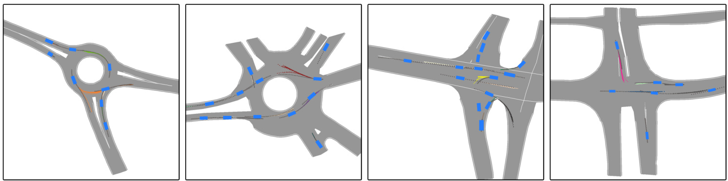
Fig. 1: Example predictions of ITRA for 3 seconds into the future based on a 1 second history. In most cases, the model is able to predict the ground truth trajectory with near certainty, but sometimes, such as when approaching a roundabout exit, there is inherent uncertainty which gives rise to multi-modal predictions. The ground truth trajectory is plotted in dark gray.
图 1: ITRA基于1秒历史数据对未来3秒的预测示例。在多数情况下,该模型能以近乎确定的概率预测真实轨迹,但在某些场景(如接近环岛出口时)会因固有不确定性产生多模态预测。真实轨迹以深灰色标出。
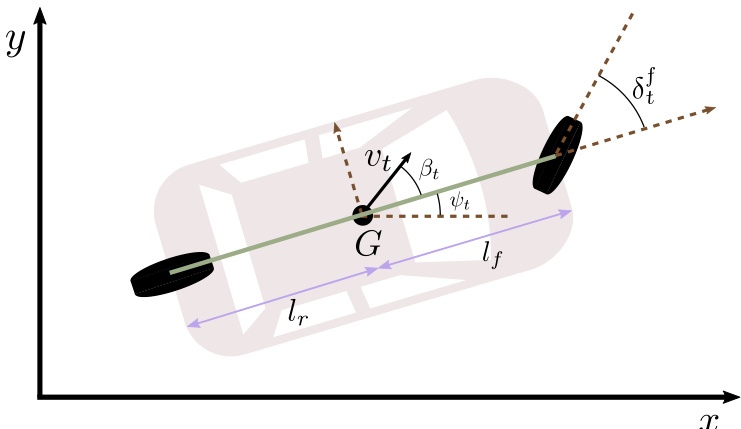
Fig. 2: [19] The kinematic bicycle model. $G$ is the geometric center of the vehicle and $v_{t}$ is its instantaneous velocity. Since our dataset does not contain entries for $\delta_{t}^{f}$ , we regard $\beta_{t}$ as steering directly, which is mathematically equivalent to setting $l_{f}=0$ . We fit $l_{r}$ by grid search for each recorded vehicle trajectory.
图 2: [19] 运动学自行车模型。$G$ 表示车辆的几何中心,$v_{t}$ 为其瞬时速度。由于数据集中未包含 $\delta_{t}^{f}$ 的条目,我们将 $\beta_{t}$ 直接视为转向角,这在数学上等价于设定 $l_{f}=0$。我们通过网格搜索为每条记录的车辆轨迹拟合 $l_{r}$ 值。
III. METHOD
III. 方法
Our model consists of a map specifying the driveable area and a composition of homogeneous agents, whose interactions are mediated by a differentiable simulator. At each timestep $t$ , each agent $i$ chooses an action $a_{t}^{i}$ , which then determines its next state according to a kinematic model $s_{t+1}^{i}~=~k i n(s_{t}^{i},a_{t}^{i})$ , which is usually the bicycle model, but we also explore some alternatives in Section IV-C. The states of all agents are pooled together to form the full state of the world $s_{t}$ , which is presented to each agent as $b_{t}^{i}$ , a rasterized, ego-centered and ego-rotated birdview image, as depicted in Figure 3. This rasterized birdview representation is commonly employed in existing models [22], [8], [11]. We choose to use three RGB channels to reduce the embedding network size. Each agent has its own hidden state $h_{t}^{i}$ , which serves as the agent’s memory, and a source of randomness ${\boldsymbol{z}}_{t}^{i}$ , which is a random variable that is used to generate the agent’s stochastic behavior. The full generative model then factorizes as follows
我们的模型包含一个指定可行驶区域的地图和一组同质智能体 (agent) ,这些智能体之间的交互通过可微分模拟器进行协调。在每个时间步 $t$ ,每个智能体 $i$ 选择一个动作 $a_{t}^{i}$ ,随后根据运动学模型 $s_{t+1}^{i}~=~k i n(s_{t}^{i},a_{t}^{i})$ 确定其下一状态——通常采用自行车模型,但我们也在第 IV-C 节探讨了其他替代方案。所有智能体的状态汇集形成全局世界状态 $s_{t}$ ,并以栅格化、自我中心且随自身旋转的鸟瞰图像 $b_{t}^{i}$ 形式呈现给每个智能体,如图 3 所示。这种栅格化鸟瞰表示法在现有模型 [22][8][11] 中被广泛采用。我们选择使用三个 RGB 通道以减少嵌入网络规模。每个智能体拥有专属的隐藏状态 $h_{t}^{i}$ 作为记忆单元,以及随机源 ${\boldsymbol{z}}_{t}^{i}$ ——该随机变量用于生成智能体的随机行为。完整的生成模型可分解如下:
$$
\begin{array}{l l}{{}}&{{(1)=\qquad\quad}}\ {{}}&{{\displaystyle\int\int\prod_{t=1}^{T}\prod_{i=1}^{N}p(z_{t}^{i})p(a_{t}^{i}|b_{t}^{i},z_{t}^{i},h_{t}^{i})p(s_{t+1}^{i}|s_{t}^{i},a_{t}^{i})d z_{1:T}^{1:N}d a_{1:T}^{1:N}}}\end{array}
$$
$$
\begin{array}{l l}{{}}&{{(1)=\qquad\quad}}\ {{}}&{{\displaystyle\int\int\prod_{t=1}^{T}\prod_{i=1}^{N}p(z_{t}^{i})p(a_{t}^{i}|b_{t}^{i},z_{t}^{i},h_{t}^{i})p(s_{t+1}^{i}|s_{t}^{i},a_{t}^{i})d z_{1:T}^{1:N}d a_{1:T}^{1:N}}}\end{array}
$$
Our model uses additional information about the environment in a form of a map rendered onto the birdview image, but for clarity we omit this from our notation.
我们的模型使用了以鸟瞰图形式渲染的环境地图作为额外信息,但为了清晰起见,我们在表示法中省略了这部分。
In ITRA, the conditional distribution of actions given latent variables and observations $p(a_{t}^{i}|b_{t}^{i},z_{t}^{i},h_{t}^{i})$ is deterministic, the distribution of the latent variables is unit Gaussian $p(z_{t}^{i})=\mathcal{N}(0,1)$ , and the distribution of states is Gaussian with a mean dictated by the kinematic model and a fixed diagonal variance $p(s_{t+1}^{i}|s_{t}^{i},a_{t}^{i})=\mathcal{N}(k i n(s_{t}^{i},a_{t}^{i}),\sigma\mathbf{I})$ , where $\sigma$ is a hyper parameter of the model.
在ITRA中,给定潜在变量和观测值的动作条件分布 $p(a_{t}^{i}|b_{t}^{i},z_{t}^{i},h_{t}^{i})$ 是确定性的,潜在变量的分布为单位高斯分布 $p(z_{t}^{i})=\mathcal{N}(0,1)$,状态分布则是高斯分布,其均值由运动学模型决定,方差为固定对角矩阵 $p(s_{t+1}^{i}|s_{t}^{i},a_{t}^{i})=\mathcal{N}(kin(s_{t}^{i},a_{t}^{i}),\sigma\mathbf{I})$,其中 $\sigma$ 是模型的超参数。
A. Differentiable Simulation
A. 可微分模拟
While the essential modeling of human behavior is performed by the VRNN generating actions, an integral part of ITRA is embedding that VRNN in a simulation consisting of the kinematic model and the procedure for generating birdview images, which is used both at training and test time. The entire model is end-to-end differentiable, allowing the parameters of the VRNN to be trained by gradient descent. For the kinematic model, this is as simple as implementing its equations of motion in PyTorch [23], but the birdview image construction is more involved.
虽然人类行为的基本建模由生成动作的VRNN完成,但ITRA的关键部分是将该VRNN嵌入到包含运动学模型和鸟瞰图生成流程的仿真系统中,这套系统在训练和测试阶段都会使用。整个模型采用端到端可微分设计,使得VRNN参数能够通过梯度下降法进行训练。对于运动学模型而言,只需在PyTorch语言[23]中实现其运动方程即可,但鸟瞰图构建过程则更为复杂。
We use PyTorch3D [24], a PyTorch-based library for differentiable rendering, to construct the birdview images. While the library primarily targets 3D applications, we obtain a simple 2D raster iz ation by applying an orthographic projection camera and a minimal shader that ignores lighting.
我们使用基于PyTorch语言的可微分渲染库PyTorch3D [24]来构建鸟瞰图。虽然该库主要面向3D应用,但通过应用正交投影相机和忽略光照的最小着色器,我们实现了简单的2D光栅化。
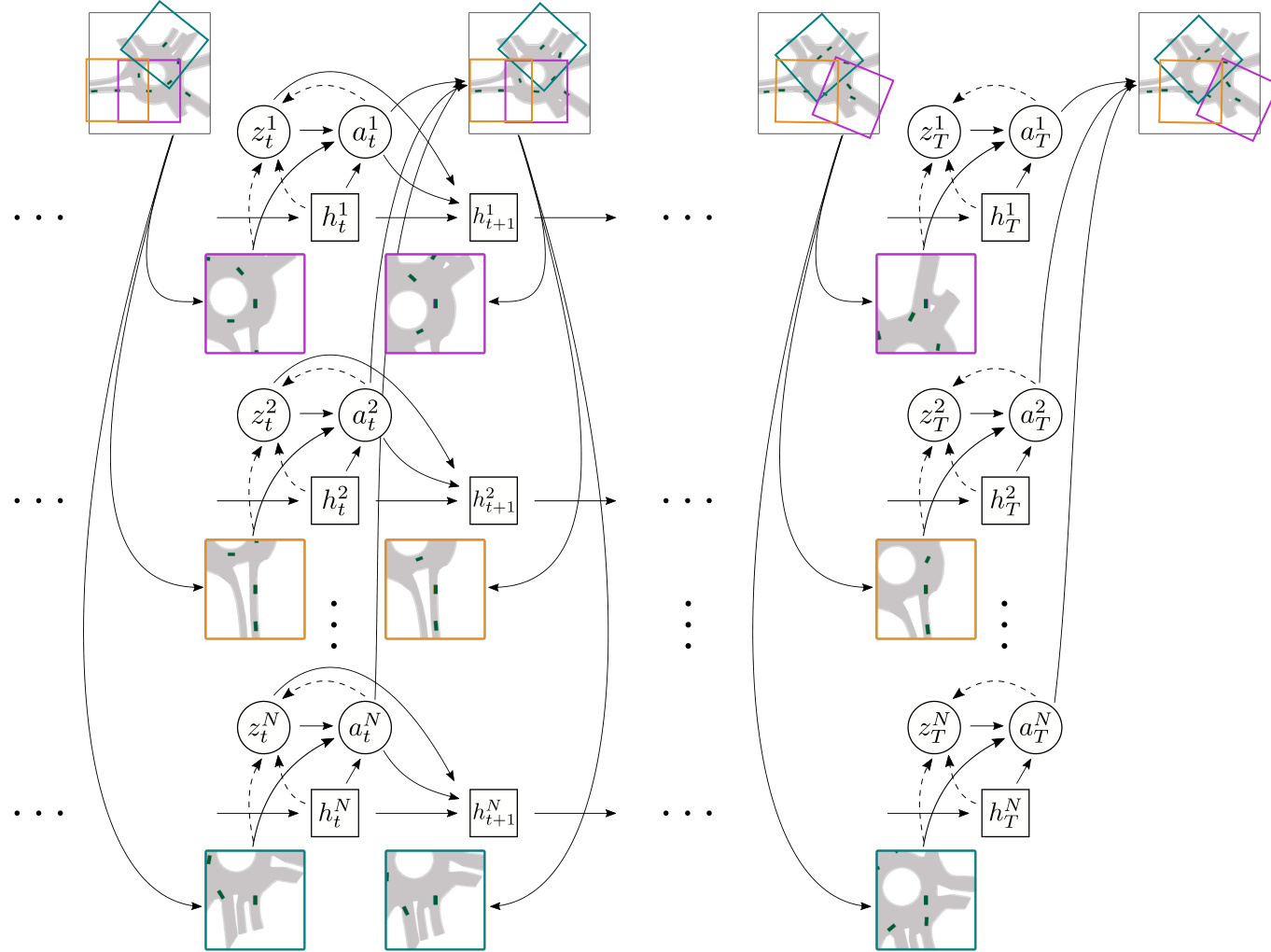
Fig. 3: A schematic illustration of ITRA’s architecture. The agents choose the actions at each time step independently from each other, obtaining information about other agents and the environment only through ego-centered birdview images. This representation naturally accommodates an unbounded, variable number of agents and time steps. The actions are translated into new agent states using a kinematic model not shown on the diagram. The colored bounding boxes illustrate each agent’s field of view in the full scene.
图 3: ITRA架构示意图。各AI智能体在每个时间步独立选择动作,仅通过以自我为中心的鸟瞰图像获取其他智能体及环境信息。这种表示方式天然支持无边界、可变数量的智能体与时间步。动作通过图中未展示的运动学模型转换为新的智能体状态。彩色边界框展示了各智能体在全场景中的视野范围。
To make the process differentiable we use the soft RGB blend algorithm [25].
为了使过程可微分,我们使用了软RGB混合算法 [25]。
B. Neural Networks
B. 神经网络
Each agent is modelled with a two-layer recurrent neural network using the gated recurrent unit (GRU) with a convolutional neural network (CNN) encoder for processing the birdview image. The remaining components are fully connected. We choose the latent dimensions to be 64 for $h$ and 2 for $z$ and we use birdview images in $256\times256$ resolution corresponding to a $100\times100$ meter area. We chose standard, well-established architectures to demonstrate that the improved performance in ITRA comes from the inclusion of a differentiable simulator.
每个智能体采用双层循环神经网络建模,使用门控循环单元 (GRU) 和卷积神经网络 (CNN) 编码器处理鸟瞰图像,其余组件为全连接结构。我们设定潜在维度为:$h$ 取64,$z$ 取2,并使用对应 $100\times100$ 米区域的 $256\times256$ 分辨率鸟瞰图像。选择这些标准成熟架构是为了证明ITRA的性能提升源于可微分模拟器的引入。
as the ground truth action extracted from the data, defining a variation al distribution $q(z_{t}^{i}|a_{t}^{i},b_{t}^{i},h_{t}^{i})$ . The ELBO is then defined as
将数据中提取的真实动作作为基础,定义一个变分分布 $q(z_{t}^{i}|a_{t}^{i},b_{t}^{i},h_{t}^{i})$ 。随后定义ELBO为
$$
\begin{array}{r}{\mathcal{L}=\displaystyle\sum_{i=1}^{N}\sum_{t=1}^{T-1}\bigg(\mathbb{E}{q(z_{t}^{i}|a_{t}^{i},b_{t}^{i},h_{t}^{i})}\left[\log p(s_{t+1}^{i}|b_{t}^{i},z_{t}^{i},h_{t}^{i})\right]}\ {-K L\left[q(z_{t}^{i}|a_{t}^{i},b_{t}^{i},h_{t}^{i})||p(z_{t}^{i})\right]\bigg),}\end{array}
$$
$$
\begin{array}{r}{\mathcal{L}=\displaystyle\sum_{i=1}^{N}\sum_{t=1}^{T-1}\bigg(\mathbb{E}{q(z_{t}^{i}|a_{t}^{i},b_{t}^{i},h_{t}^{i})}\left[\log p(s_{t+1}^{i}|b_{t}^{i},z_{t}^{i},h_{t}^{i})\right]}\ {-K L\left[q(z_{t}^{i}|a_{t}^{i},b_{t}^{i},h_{t}^{i})||p(z_{t}^{i})\right]\bigg),}\end{array}
$$
where $s_{t}^{i}$ are the ground truth states obtained from the dataset. This is the standard setting for training conditional variation al recurrent neural networks (CVRNNs), with a caveat that we introduce a distinction between actions and states.
其中 $s_{t}^{i}$ 是从数据集中获取的真实状态。这是训练条件变分循环神经网络 (CVRNN) 的标准设置,但需要注意我们引入了动作和状态之间的区分。
C. Training and Losses
C. 训练与损失
We train all the network components jointly from scratch using the evidence lower bound (ELBO) as the optimization objective. For this purpose, we use an inference network that parameter ize s a diagonal Gaussian distribution over $z$ given the current observation and recurrent state, as well
我们使用证据下界(ELBO)作为优化目标,从头开始联合训练所有网络组件。为此,我们采用了一个推理网络,该网络基于当前观测值和循环状态对$z$进行对角高斯分布的参数化。
D. Conditional Predictions
D. 条件预测
Typically, trajectory prediction tasks are defined as predicting a future trajectory $T_{o b s}+1:T$ based on a past trajectory $1:T_{o b s}$ . Predicting trajectories from a single frame is unnecessarily difficult and using Eq. 2 naively with a randomly initialized recurrent state $h_{1}$ destabilize s the training process and leads to poor predictions. To make sure the recurrent state is seeded well, we employ teacher forcing for states $s_{t}$ at time $1:T_{o b s}$ but not after $T_{o b s}$ , which corresponds to performing an inference over the state of $h_{T_{o b s}}$ given observations from previous time steps. We do this both at training and test time.
通常,轨迹预测任务被定义为根据过去轨迹 $1:T_{obs}$ 预测未来轨迹 $T_{obs}+1:T$。从单帧预测轨迹会不必要地增加难度,若直接使用公式2并随机初始化循环状态 $h_1$,会导致训练过程不稳定并产生较差预测结果。为确保循环状态良好初始化,我们对 $1:T_{obs}$ 时段的状态 $s_t$ 采用教师强制策略,但在 $T_{obs}$ 之后不使用。这相当于基于先前时间步的观测值对 $h_{T_{obs}}$ 状态进行推断。该策略在训练和测试阶段均被采用。
IV. EXPERIMENTAL RESULTS
IV. 实验结果
For our experiments, we use the INTERACTION dataset [16], which consists of about 10 hours of traffic data containing 36,000 vehicles recorded in 11 locations around the world at intersections, roundabouts, and highway ramps. Our model achieves state-of-the-art performance, as reported in Table I, and we also provide in Table II a more detailed breakdown of the scores it achieves across different scenes to enable a more fine-grained analysis. Finally, we ablate the kinematic bicycle model and the birdview generation for future times, the two key components of ITRA’s simulation, showing that both of them are necessary to achieve the reported performance.
在我们的实验中,我们使用了INTERACTION数据集[16],该数据集包含约10小时的交通数据,记录了全球11个地点(包括交叉路口、环岛和高速公路匝道)的36,000辆车辆。如表I所示,我们的模型实现了最先进的性能,并在表II中提供了更详细的分数细分,以便进行更细粒度的分析。最后,我们对ITRA仿真中的两个关键组件(运动学自行车模型和未来时间的鸟瞰图生成)进行了消融实验,结果表明两者对于实现所报告的性能都是必要的。
Following the recommendation of [11], we apply classmates forcing, where the actions and states of all agents other than the ego vehicle are fixed to ground truth at training time and not generated by the VRNN, which allows us to use batches of diverse examples and stabilizes training. At test time, we predict the motion of all agents in the scene, including bicycles/pedestrians (which are not distinguished from each other in the dataset). For simplicity, we use the same model trained on vehicles to predict all agent types, noting that it could be possible to obtain further improvements by training a separate model for bicycles/pedestrians. We trained all the model components jointly from scratch using the ADAM optimizer [26] with the standard learning rate of 3e-4, using gradient clipping and a batch size of 8. We found the training to be relatively stable with respect to other hyper parameters and have not performed extensive tuning. The training process takes about two weeks on a single NVIDIA Tesla P100 GPU.
遵循[11]的建议,我们采用同学强制(classmates forcing)策略:在训练时将非自车(non-ego vehicle)的所有智能体动作和状态固定为真实值而非由VRNN生成,这使我们能使用多样化样本批次并稳定训练。测试时,我们预测场景中所有智能体(包括自行车/行人,该数据集未对二者区分)的运动。为简化流程,我们使用同一套针对车辆训练的模型预测所有智能体类型,但指出通过为自行车/行人单独训练模型可能获得进一步改进。我们使用ADAM优化器[26]以3e-4标准学习率从头联合训练所有模型组件,采用梯度裁剪和批次大小为8的配置。训练过程对其他超参数相对稳定,未进行大量调参。在单块NVIDIA Tesla P100 GPU上训练耗时约两周。
Finally, we note that we compute ground truth actions used as input to the inference network based on a sequence of ground truth states, independently of what the model predicts at earlier times. We found that this greatly speeds up training and leads to better final performance.
最后,我们注意到,我们基于一系列真实状态计算作为推理网络输入的真实动作,而不依赖于模型在早期时间点的预测。我们发现这能显著加快训练速度并带来更好的最终性能。
A. Evaluation Metrics
A. 评估指标
where $(x_{t}^{i},y_{t}^{i})$ is the ground truth position of agent $i$ at time $t$ . When multiple trajectory predictions can be generated,
其中 $(x_{t}^{i},y_{t}^{i})$ 是智能体 $i$ 在时间 $t$ 的真实位置。当可以生成多个轨迹预测时,
TABLE I: Validation set prediction errors on the INTERACTION Dataset evaluated with the suggested train/validation split. The evaluation is based on six samples, where for each example the trajectory with the smallest error is selected, independently for ADE and FDE. ReCoG only makes deterministic predictions, so its performance would be the same with a single sample. The values for baselines are as reported by their original authors, with the exception of DESIRE and MultiPath, where we present the results reported in [9].
表 1: 基于建议的训练/验证划分在INTERACTION数据集上验证集的预测误差评估。该评估基于六个样本,其中每个样本独立选取ADE和FDE误差最小的轨迹。ReCoG仅进行确定性预测,因此其单样本性能保持不变。基线数据来源于原作者报告,但DESIRE和MultiPath的结果采用[9]中报告的数据。
| 方法 | minADE6 | min FDE6 |
|---|---|---|
| DESIRE [5] | 0.32 | 0.88 |
| MultiPath [3] | 0.30 | 0.99 |
| TNT [9] | 0.21 | 0.67 |
| ReCoG [17] | 0.19 | 0.65 |
| ITRA (ours) | 0.17 | 0.49 |
TABLE II: Breakdown of ITRA’s performance across individual scenes in the INTERACTION dataset. We present evaluation of a single model trained on all scenes jointly, noting that fine-tuning on individual scenes can further improve performance. CHN Merging ZS, which is a congested highway where predictions are relatively easy, is overrepresented in the dataset, lowering the average error across scenes.
表 II: ITRA 在 INTERACTION 数据集中各场景的性能细分。我们展示了在所有场景上联合训练的单一模型评估结果,并指出针对单个场景进行微调可以进一步提升性能。CHN Merging ZS 是一条拥堵的高速公路场景,其预测相对容易,但该场景在数据集中占比过高,从而拉低了跨场景的平均误差。
| 场景 | minADE6 | min FDE6 | MFD6 |
|---|---|---|---|
| CHN Merging ZS | 0.127 | 0.356 | 2.157 |
| CHN RoundaboutLN | 0.199 | 0.549 | 2.354 |
| DEUI Merging MT | 0.226 | 0.678 | 2.178 |
| DEURoundaboutOF | 0.283 | 0.766 | 3.389 |
| USAIntersectionEPO | 0.215 | 0.640 | 3.008 |
| USAIntersectionEP1 | 0.234 | 0.678 | 2.974 |
| USAIntersection GL | 0.203 | 0.611 | 2.750 |
| USAIntersectionMA | 0.212 | 0.634 | 3.430 |
| USARoundaboutEP | 0.234 | 0.690 | 3.094 |
| USARoundaboutFT | 0.219 | 0.661 | 2.932 |
| USARoundaboutSR | 0.178 | 0.525 | 2.451 |
the predicted trajectory with the smallest error is selected for evaluation. In either case, the errors are averaged across agents and test examples.
选择误差最小的预测轨迹进行评估。无论哪种情况,误差都会在智能体和测试样本间取平均值。
$$
\begin{array}{l}{\displaystyle\operatorname*{min}\mathrm{ADE}{K}=\frac{1}{N}\sum_{i=1}^{N}\operatorname*{min}{k}\mathrm{ADE}{k}^{i}}\ {\displaystyle\operatorname*{min}\mathrm{FDE}{K}=\frac{1}{N}\sum_{i=1}^{N}\operatorname*{min}{k}\mathrm{FDE}_{k}^{i}}\end{array}
$$
$$
\begin{array}{l}{\displaystyle\operatorname*{min}\mathrm{ADE}{K}=\frac{1}{N}\sum_{i=1}^{N}\operatorname*{min}{k}\mathrm{ADE}{k}^{i}}\ {\displaystyle\operatorname*{min}\mathrm{FDE}{K}=\frac{1}{N}\sum_{i=1}^{N}\operatorname*{min}{k}\mathrm{FDE}_{k}^{i}}\end{array}
$$
Note that these metrics only score position and not orientation or speed predictions, so most trajectory prediction models only generate position coordinates.
请注意,这些指标仅评估位置预测,而不涉及方向或速度预测,因此大多数轨迹预测模型仅生成位置坐标。
While not directly measuring performance, a useful metric for tracking the diversity of predicted trajectories is the Maximum Final Distance (MFD)
虽然不直接衡量性能,但最大终点距离 (MFD) 是追踪预测轨迹多样性的有效指标
$$
\mathrm{MFD}{K}=\frac{1}{N}\sum_{i=1}^{N}\operatorname*{max}{k,l}\sqrt{(x_{T}^{i,k}-x_{T}^{i,l})^{2}+(y_{T}^{i,k}-y_{T}^{i,l})^{2}},
$$
$$
\mathrm{MFD}{K}=\frac{1}{N}\sum_{i=1}^{N}\operatorname*{max}{k,l}\sqrt{(x_{T}^{i,k}-x_{T}^{i,l})^{2}+(y_{T}^{i,k}-y_{T}^{i,l})^{2}},
$$
which we primarily use to diagnose when the model collapses onto deterministic predictions.
我们主要用它来诊断模型何时坍缩为确定性预测。
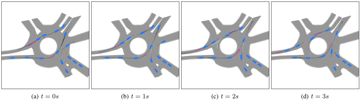
Fig. 4: A sequence of 4 subsequent prediction snapshots spaced 1 second apart. For each vehicle in the scene we show 10 sampled predictions over the subsequent 3 seconds based on the previous 1 second. Notice the car that just entered the roundabout from top-right in 4a, for which ITRA predicts that it will go forward in the roundabout, and as it enters the roundabout in $_{\mathrm{4c}}$ , the prediction diversifies to include both exiting the roundabout and continuing the turn, finally matching the ground truth trajectory (in dark grey) in 4d once the car started turning.
图 4: 间隔1秒的连续4个预测快照序列。针对场景中每辆车,我们基于前1秒数据展示了未来3秒内的10条采样预测轨迹。注意4a中刚从右上角进入环岛的车辆:ITRA最初预测其将直行通过环岛,当车辆进入环岛时(4c),预测轨迹开始分化出"驶离环岛"和"继续转弯"两种可能,最终在车辆开始转弯时(4d)与真实轨迹(深灰色)完全吻合。
B. Ablations on Future Birdview Images
B. 未来鸟瞰图像的消融实验
A key aspect of ITRA is the ongoing simulation throughout the future time steps, generating updated birdview images providing feedback to the agents. While powerful, this simulation complicates the software architecture and is computationally expensive. In this section, we analyze two ablations, which remove the dynamic feedback aspect provided by future birdview images.
ITRA的一个关键方面是在未来时间步长中持续进行仿真,生成更新的鸟瞰图像为智能体提供反馈。虽然功能强大,但这种仿真使软件架构复杂化且计算成本高昂。本节我们分析两种消融实验,它们移除了未来鸟瞰图像提供的动态反馈特性。
In the first ablation, we use normal birdview images up to time $T_{o b s}$ and then blank images subsequently, both at training and test time. This removes any feedback and roughly corresponds to models that predict the entire future trajectory in a single step based on past observations [5], [6], [7], [8], [9], albeit with a suboptimal neural architecture. In the second ablation, we perform teacher forcing at training time, fixing the agent’s state and the birdview image to the ground truth values at each time step. In both cases, we find that the ablated model performs significantly worse and exhibits no prediction diversity, as shown in Figure 5.
在第一次消融实验中,我们在训练和测试时都使用截至时间 $T_{o b s}$ 的正常鸟瞰图像,之后使用空白图像。这移除了所有反馈,大致对应于基于过去观测在单一步骤中预测整个未来轨迹的模型 [5]、[6]、[7]、[8]、[9],尽管使用了次优的神经网络架构。在第二次消融实验中,我们在训练时执行教师强制 (teacher forcing),将智能体的状态和鸟瞰图像固定为每个时间步的真实值。在这两种情况下,我们发现消融模型表现明显更差,并且没有预测多样性,如图 5 所示。
C. Alternative Kinematic Models
C. 替代运动学模型
While our approach relies on the kinematic bicycle model, we have also investigated several alternatives. In the simplest one, which we call the un constrained model, the action is the delta between subsequent state vectors.
虽然我们的方法依赖于运动学自行车模型 (kinematic bicycle model),但我们也研究了其他几种替代方案。其中最简单的一种称为无约束模型 (unconstrained model),其动作是后续状态向量之间的差值。
$$
a_{t}^{i}=(x_{t+1}^{i}-x_{t}^{i},y_{t+1}^{i}-y_{t}^{i},\psi_{t+1}^{i}-\psi_{t}^{i},v_{t+1}^{i}-v_{t}^{i})
$$
$$
a_{t}^{i}=(x_{t+1}^{i}-x_{t}^{i},y_{t+1}^{i}-y_{t}^{i},\psi_{t+1}^{i}-\psi_{t}^{i},v_{t+1}^{i}-v_{t}^{i})
$$
We have found that the un constrained model not only performs worse in terms of the evaluation metrics outlined in Section IV-A, but also that it sometimes generates physically implausible trajectories, where the cars are driving sideways or even spinning. We speculate that this behavior makes it difficult for the model to use the birdview images as an effective feedback mechanism.
我们发现,无约束模型不仅在第四-A节概述的评估指标上表现更差,有时还会生成物理上不合理的轨迹,例如车辆横向行驶甚至打转。我们推测这种行为使得模型难以将鸟瞰图作为有效的反馈机制。
We have also tried using displacements in $x$ and $y$ as the action space, letting the bicycle model fill in the associated orientation and speed, which we refer to as the displacement model. Finally, we tried oriented versions of both the un constrained and the displacement models, where the $x{-}y$ coordinates rotate with the ego vehicle. We found the bicycle model to perform much better than any of the alternatives, as shown in Figure 6.
我们还尝试使用$x$和$y$方向的位移作为动作空间,让自行车模型填充相关的方向和速度,我们称之为位移模型。最后,我们尝试了无约束模型和位移模型的定向版本,其中$x{-}y$坐标随自车旋转。如图6所示,我们发现自行车模型的表现远优于其他替代方案。
V. RELATED WORK
V. 相关工作
The literature on trajectory prediction is vast. Due to space constraints, we narrow our focus to methods that predict distributions over future trajectories with deep generative models, which currently achieve state of the art performance, although even there our coverage is far from complete. For a more comprehensive survey of the field see [27].
关于轨迹预测的文献浩如烟海。由于篇幅限制,我们仅聚焦于使用深度生成模型预测未来轨迹分布的方法,这类方法目前实现了最先进的性能,即便如此我们的综述仍远未全面。更完整的领域综述请参阅[27]。
The first paper we are aware of to apply CVAEs to the task of motion prediction is [28], which predicts the movement of pixels in a video of one second into the future from a single frame. The paper is not explicitly concerned with predicting the trajectories of humans navigating through space. One of the most influential papers applying CVAEs to the task of predicting human trajectories is DESIRE [5], where like in ITRA the information about the environment is encoded in a birdview image processed by a CNN and a latent random variable is used to generate diverse trajectories. Unlike in ITRA, there is no mechanism for the agents to interact with each other or with the environment past the initial frame.
我们已知首篇将CVAE (Conditional Variational Autoencoder) 应用于运动预测任务的论文是[28],该研究通过单帧画面预测视频中未来一秒内的像素移动。该论文并未明确关注预测人类在空间中的移动轨迹。应用CVAE预测人类轨迹最具影响力的论文之一是DESIRE [5],其与ITRA类似,通过CNN处理鸟瞰图编码环境信息,并利用潜变量生成多样化轨迹。但与ITRA不同的是,DESIRE没有设计智能体在初始帧之后与环境或其他智能体交互的机制。
The most popular alternative to VAEs are generative adversarial networks (GANs) [29], which have been been applied to trajectory prediction in papers such as Social GAN [7], SoPhie [6], and [8]. These approaches differ in how they construct the loss functions and how they encode the information about the past, but in all of them predictions for different agents are generated independently, by decoding a random variable with an RNN.
VAE最流行的替代方案是生成对抗网络 (GAN) [29],已在Social GAN [7]、SoPhie [6] 和 [8] 等论文中应用于轨迹预测。这些方法的差异在于损失函数的构建方式和对历史信息的编码机制,但所有方法都通过RNN解码随机变量来独立生成不同智能体的预测结果。
In PRECOG [10], future trajectories of agents are predicted jointly using normalizing flows, another family of deep generative models, to construct a distribution over predicted trajectories. Normalizing flows allow for easy evaluation of likelihoods, which is necessary for model learning, but at the expense of being less flexible than models based on VAEs and GANs. PRECOG models the interactions between agents explicitly, which means it is only applicable to a fixed (or limited) number of agents, while in our model the interactions are mediated through a birdview image, which has a fixed size independent of the number of agents and therefore our model can handle an unbounded number of agents. In PRECOG, prediction is bundled with LiDAR-based detection, which necessitates the use of ad-hoc heuristics to project future LiDAR readings, and precludes it being applied to datasets that do not contain LiDAR readings, such as INTERPRET.
在PRECOG [10]中,研究者使用归一化流(normalizing flows)这一深度生成模型家族来联合预测智能体的未来轨迹,构建预测轨迹的概率分布。归一化流便于评估似然值,这对模型学习至关重要,但代价是其灵活性不如基于VAE和GAN的模型。PRECOG显式建模智能体间的交互,这意味着它仅适用于固定(或有限)数量的智能体;而我们的模型通过鸟瞰图图像中介交互,该图像具有与智能体数量无关的固定尺寸,因此能处理无限数量的智能体。PRECOG将预测与基于LiDAR的检测捆绑,这需要使用临时启发式方法来预测未来LiDAR读数,导致其无法应用于不含LiDAR读数的数据集(如INTERPRET)。

Fig. 5: Comparison of a normal ITRA training process with one that uses a blank birdview image for future steps and with one that uses teacher forcing, i.e. uses birdview images representing ground truth at training time. Both of these ablations produce inaccurate results and essentially no diversity in predictions, indicating that it is necessary to generate birdview images dynamically both at training and test time. With teacher forcing the training loss is so small that it blends in with the x axis.
图 5: 正常ITRA训练过程与使用空白鸟瞰图进行未来步骤预测的训练过程对比,以及与使用教师强制(teacher forcing)(即在训练时使用代表真实值的鸟瞰图)的训练过程对比。这两种消融实验均产生了不准确的结果,且预测结果基本无多样性,表明在训练和测试时动态生成鸟瞰图是必要的。使用教师强制时,训练损失极小,几乎与x轴重合。
Multiple Futures Prediction [11] also predicts the trajectories of different agents jointly, but instead of using continuous latent variables it uses a single discrete variable per agent with a small number of possible values. This allows the model to capture a fixed number of modes in predictions, but is not enough to capture all possible aspects of non-Gaussian variability. It also does not model vehicle orientations. The paper was published before the INTERACTION dataset was released so does not include the model’s performance on it and we found the associated code difficult to adapt to this dataset for direct comparison.
多未来预测 [11] 同样联合预测不同智能体的轨迹,但它不使用连续潜变量,而是为每个智能体分配一个离散变量,该变量仅有少量可能取值。这种方法能捕捉预测中的固定数量模态,但不足以涵盖非高斯变异性所有可能的方面。该模型也未对车辆方向进行建模。由于论文发表于INTERACTION数据集发布之前,因此未包含模型在该数据集上的性能表现,且我们发现相关代码难以适配该数据集以进行直接比较。

Fig. 6: Training curves for ITRA with different kinematic models. The bicycle model with its standard action space outperforms all the alternatives by a substantial margin. We smoothed the curves using exponential moving average to make the plots more legible, leaving the raw measurements faded out.
图 6: 不同运动学模型下ITRA的训练曲线。采用标准动作空间的自行车模型显著优于其他所有方案。我们使用指数移动平均对曲线进行平滑处理以提高可读性,原始测量数据以淡色显示。
TrafficSim [30], created independently of and concurrently with our work, proposes a model very similar to ITRA, modelling different vehicles with CVRNNs. It does not utilize differentiable rendering, instead encoding only the static portion of the map as a rasterized birdview image and employing a graph neural network to encode agent interactions. It is not clear to us whether TrafficSim employs any kinematic constraints on the motion of vehicles. The implementation was not released and the paper only reports performance on a proprietary dataset, so we were not able to compare the performance of TrafficSim and ITRA.
TrafficSim [30] 是与我们的工作独立且同时期提出的一个与ITRA非常相似的模型,它使用CVRNN对不同车辆进行建模。该方法未采用可微分渲染技术,仅将地图静态部分编码为栅格化鸟瞰图,并通过图神经网络处理智能体间的交互关系。目前尚不明确TrafficSim是否对车辆运动施加了任何运动学约束。由于未公开实现代码且论文仅报告了在私有数据集上的性能表现,我们无法对TrafficSim与ITRA的性能进行直接比较。
VI. DISCUSSION
VI. 讨论
The ultimate use cases for multi-agent generative behavioral models like ITRA require additional future work. One problem we found is that when trained on the INTERACTION dataset, ITRA fails to generalize perfectly to significantly different road topologies, sometimes going offroad in non-sensical ways. This issue will most likely be overcome by using additional training data with extensive coverage of road topologies. In recent years, many suitable datasets have been publicly released [31], [32], [33], [34], [35] and training ITRA on them is one of our directions for future work. We note, however, that those datasets come in substantially different formats, particularly regarding the map specification, which requires a significant amount of work to incorporate them into our differentiable simulator.
像ITRA这样的多智能体生成行为模型的最终应用场景还需要进一步的研究。我们发现的一个问题是,当在INTERACTION数据集上训练时,ITRA无法完美泛化到显著不同的道路拓扑结构,有时会以不合理的方式偏离道路。这个问题很可能通过使用覆盖广泛道路拓扑的额外训练数据来解决。近年来,许多合适的数据集已公开发布[31]、[32]、[33]、[34]、[35],在这些数据集上训练ITRA是我们未来的研究方向之一。然而,我们注意到这些数据集的格式差异很大,特别是在地图规范方面,需要大量工作才能将它们整合到我们的可微分模拟器中。
While the typical use-case for predictive trajectory models is to determine safe areas in path planners, ITRA itself could be used as a planner providing a nominal trajectory for a low-level controller. While this is not necessarily desirable for deployment in autonomous vehicles (AVs), since it imitates both the good and the bad aspects of human behavior, that is precisely what is the goal when building non-playable characters (NPCs) simulating human drivers for training and testing AVs in a virtual environment. We are currently interfacing ITRA with CARLA [36] to control such NPCs, noting that this can be done with any other simulator such as TORCS [37], LGSVL [38], or NVIDIA’s Drive Constellation. The main requirement is to provide a lowlevel controller that can steer the car to follow the trajectory specified by ITRA.
虽然预测轨迹模型的典型用例是在路径规划器中确定安全区域,但ITRA本身可作为规划器为底层控制器提供标称轨迹。尽管这对自动驾驶汽车(AV)部署未必理想(因为它同时模仿了人类行为的优缺点),但这恰恰是构建非玩家角色(NPC)时的目标——在虚拟环境中模拟人类驾驶员以训练和测试AV。我们正将ITRA与CARLA [36]对接来控制此类NPC,值得注意的是,该方案也适用于其他仿真器如TORCS [37]、LGSVL [38]或NVIDIA Drive Constellation。核心要求是提供能操控车辆跟随ITRA指定轨迹的底层控制器。
Finally, a drawback of ITRA when used for such applications is that its behavior cannot directly be controlled with high-level commands such as picking the exit to take at a roundabout or yielding to another vehicle. However, since the distribution over trajectories it predicts contains all the behaviors it was exposed to in the dataset, in principle it can be conditioned on achieving certain outcomes, yielding a complete distribution over human-like trajectories that achieve the specified goal. In practice, this is difficult for computational reasons, but can be overcome with techniques such as amortized rejection sampling [39], [40], which we are currently working on utilizing in this context.
最后,ITRA在此类应用中的一个缺点是,其行为无法通过高级指令直接控制,例如选择环岛出口或礼让其他车辆。但由于其预测的轨迹分布涵盖了数据集中所有观察到的行为,理论上可以通过条件约束实现特定目标,从而生成符合指定要求的人类驾驶风格轨迹全集。实际应用中,由于计算复杂度限制这一过程存在困难,但可通过摊销拒绝采样 (amortized rejection sampling) [39][40] 等技术解决——这正是我们当前在该领域重点攻关的方向。
APPENDIX
附录
A. Bicycle Model Equations
A. 自行车模型方程
Usually the action space of the kinematic bicycle model consists of acceleration and steering angle and it has two parameters defining the distances from the geometric center to front and rear axes. However, since we do not observe the wheel position and do not know where the axes are, the steering angle can not be determined, so instead we define the steering action to directly control the angle $\beta$ between the vehicle’s orientation and its instantaneous velocity.
通常,运动自行车模型的动作空间由加速度和转向角组成,并有两个参数定义从几何中心到前后轴的距离。然而,由于我们无法观察到车轮位置且不知道轴的具体位置,转向角无法确定,因此我们改为定义转向动作直接控制车辆方向与其瞬时速度之间的角度 $\beta$。
The continuous time equations of motion for the bicycle
自行车的连续时间运动方程
model are:
模型包括:
$$
\begin{array}{l}{\displaystyle\dot{v_{t}}=\alpha_{t}}\ {\displaystyle\dot{x_{t}}=v_{t}\cos(\psi_{t}+\beta_{t})}\ {\displaystyle\dot{y_{t}}=v_{t}\sin(\psi_{t}+\beta_{t})}\ {\displaystyle\dot{\psi_{t}}=\frac{v_{t}}{l_{r}}\sin(\beta_{t}).}\end{array}
$$
$$
\begin{array}{l}{\displaystyle\dot{v_{t}}=\alpha_{t}}\ {\displaystyle\dot{x_{t}}=v_{t}\cos(\psi_{t}+\beta_{t})}\ {\displaystyle\dot{y_{t}}=v_{t}\sin(\psi_{t}+\beta_{t})}\ {\displaystyle\dot{\psi_{t}}=\frac{v_{t}}{l_{r}}\sin(\beta_{t}).}\end{array}
$$
The action space $a_{t}=\left(\alpha_{t},\beta_{t}\right)$ consists of the acceleration and steering angle applied to the center of the vehicle. We then use the following disc ret i zed version of these equations:
动作空间 $a_{t}=\left(\alpha_{t},\beta_{t}\right)$ 由施加在车辆中心的加速度和转向角组成。我们随后使用以下离散化版本的方程:
$$
\begin{array}{r l}&{v_{t}=v_{t-1}+\alpha_{t}\Delta_{t}}\ &{x_{t}=x_{t-1}+v_{t}\cos(\psi_{t-1}+\beta_{t})\Delta_{t}}\ &{y_{t}=y_{t-1}+v_{t}\sin(\psi_{t-1}+\beta_{t})\Delta_{t}}\ &{\psi_{t}=\psi_{t-1}+\displaystyle\frac{v_{t}}{l_{r}}\sin(\beta_{t})\Delta_{t}.}\end{array}
$$
$$
\begin{array}{r l}&{v_{t}=v_{t-1}+\alpha_{t}\Delta_{t}}\ &{x_{t}=x_{t-1}+v_{t}\cos(\psi_{t-1}+\beta_{t})\Delta_{t}}\ &{y_{t}=y_{t-1}+v_{t}\sin(\psi_{t-1}+\beta_{t})\Delta_{t}}\ &{\psi_{t}=\psi_{t-1}+\displaystyle\frac{v_{t}}{l_{r}}\sin(\beta_{t})\Delta_{t}.}\end{array}
$$
B. Fitting the Bicycle Model
B. 自行车模型拟合
The dataset contains a sequence of states for each vehicle, but not directly the actions of the bicycle model. To recover the actions, we find the values that match the displacements recorded in the dataset. Specifically, we compute the acceleration and steering according to the following equations, for $t>1$ :
该数据集包含每辆车的状态序列,但不直接包含自行车模型的动作。为了还原这些动作,我们寻找与数据集中记录的位移相匹配的数值。具体来说,对于$t>1$的情况,我们根据以下公式计算加速度和转向角度:
$$
\begin{array}{r l r}&{\displaystyle\alpha_{t}=\frac{1}{\Delta_{t}}(\frac{1}{\Delta_{t}}\sqrt{(x_{t}^{g.t.}-x_{t-1})^{2}+(y_{t}^{g.t.}-y_{t-1})^{2}}-v_{t-1})}&\ &{\quad}&{(12}\ &{\displaystyle\beta_{t}=\mathrm{atan}2(\frac{1}{\Delta_{t}}(y_{t}^{g.t.}-y_{t-1}),\frac{1}{\Delta_{t}}(x_{t}^{g.t.}-x_{t-1}))-\psi_{t-1},}\end{array}
$$
$$
\begin{array}{r l r}&{\displaystyle\alpha_{t}=\frac{1}{\Delta_{t}}(\frac{1}{\Delta_{t}}\sqrt{(x_{t}^{g.t.}-x_{t-1})^{2}+(y_{t}^{g.t.}-y_{t-1})^{2}}-v_{t-1})}&\ &{\quad}&{(12}\ &{\displaystyle\beta_{t}=\mathrm{atan}2(\frac{1}{\Delta_{t}}(y_{t}^{g.t.}-y_{t-1}),\frac{1}{\Delta_{t}}(x_{t}^{g.t.}-x_{t-1}))-\psi_{t-1},}\end{array}
$$
where $g.t$ . superscript indicates that the values are the ground truth from the dataset, otherwise they are obtained from the previous time step.
其中 $g.t$ 上标表示这些值来自数据集的真实标注 (ground truth) ,否则它们是从前一个时间步获得的。
The bicycle model fits the observed trajectories closely but not exactly. We define the loss measuring how well the bicycle model fits a given trajectory as
自行车模型与观测轨迹高度吻合但并非完全一致。我们将衡量自行车模型与给定轨迹拟合程度的损失定义为
$$
L_{b i c y c l e-f i t}=\operatorname*{max}{t\in{2,...,T}}2(1-\cos(\psi_{t}-\psi_{t}^{g.t.})),
$$
$$
L_{b i c y c l e-f i t}=\operatorname*{max}{t\in{2,...,T}}2(1-\cos(\psi_{t}-\psi_{t}^{g.t.})),
$$
which is chosen to symmetrically increase with the discrepancy angle in both directions, also to be $2\pi$ -periodic.
该函数被设计为随着差异角在双向对称增加,并且保持 $2\pi$ 周期性。
The one missing parameter is $l_{r}$ , which is not available in the dataset. To find the corresponding values, we perform a grid search on $l_{r}^{i}$ in order to minimize $L_{b i c y c l e-f i t}^{i}$ separately for each vehicle . We search in $1~\mathrm{cm}$ increments up to half the vehicle length. The histogram of the resulting values of $l_{r}$ is shown in Figure 7. Using this procedure, we achieve a near-perfect fit of the trajectories recorded in the dataset.
缺失的参数是 $l_{r}$,该参数在数据集中不可用。为了找到对应值,我们对 $l_{r}^{i}$ 进行网格搜索,以分别最小化每辆车的 $L_{b i c y c l e-f i t}^{i}$。搜索步长为 $1~\mathrm{cm}$,最大搜索范围为车长的一半。图 7 展示了所得 $l_{r}$ 值的分布直方图。通过此方法,我们实现了对数据集中记录轨迹的近乎完美拟合。