Improving the Cluster Structure Extracted from OPTICS Plots

改进从 OPTICS 图中提取的聚类结构

Erich Schubert and Michael Gertz

Erich Schubert 和 Michael Gertz

Heidelberg University {schubert,gertz}@informatik.uni-heidelberg.d

海德堡大学 {schubert,gertz}@informatik.uni-heidelberg.d

Abstract. Density-based clustering is closely associated with the two algorithms DBSCAN and OPTICS. While the first finds clusters connected at a single density threshold, the latter allows the extraction of a cluster hierarchy based on different densities. Extraction methods for clusters from OPTICS rely on an intermediate representation, known as the OPTICS plot. In this plot, which can be seen as a density profile of the data set, valleys (areas of higher density) are associated with clusters. Multiple methods for automatic detecting such valleys have been proposed, but all of them tend to produce a particular artifact, where some point is included in the cluster that may be far away from the remainder. In this article, we will discuss this commonly seen artifact, and propose a simple but sound way of removing the artifacts. At the same time, this change is minimally invasive, and tries to keep the existing algorithms largely intact for future study.

摘要。基于密度的聚类与 DBSCAN 和 OPTICS 这两种算法密切相关。前者在单一密度阈值下找到连接的聚类，而后者允许基于不同密度提取聚类层次结构。从 OPTICS 中提取聚类的方法依赖于一种中间表示，称为 OPTICS 图。在该图中，可以将数据集视为密度剖面，谷值（高密度区域）与聚类相关联。已经提出了多种自动检测此类谷值的方法，但所有这些方法都倾向于产生一种特定的伪影，其中某些点可能包含在远离其余部分的聚类中。在本文中，我们将讨论这种常见的伪影，并提出一种简单但有效的方法来去除这些伪影。同时，这种改变是微创的，并试图保持现有算法基本不变，以便未来研究。

1 Introduction

1 引言

Cluster analysis is the task of discovering previously unknown structure in a data set, and belongs to the “unsupervised learning” subdomain of data mining where no labeled data is available yet. It can be used to infer an initial labeling of the data, but clustering results tend to not be reliable enough to automate such use. But it can be used in explorative data analysis to assist the user in discovering patterns that may lead to meaningful labels after formalization. For example, a clustering might suggest three subtypes of a disease to the user, and clinical verification may be able to confirm two of these three subtypes with appropriate thresholds to differentiate them. Here, the clustering itself does not need to produce “perfect” results, but it was used to find a hypothesis.

聚类分析是发现数据集中先前未知结构的任务，属于数据挖掘中的“无监督学习”子领域，其中尚未有标注数据可用。它可以用于推断数据的初始标注，但聚类结果往往不够可靠，无法自动化此类用途。然而，它可以用于探索性数据分析，帮助用户发现可能在形式化后产生有意义标签的模式。例如，聚类可能向用户建议某种疾病的三种亚型，而临床验证可能能够确认其中两种亚型，并通过适当的阈值来区分它们。在这里，聚类本身不需要产生“完美”的结果，而是用于发现假设。

While clustering is considered an unsupervised task—it cannot learn from labels, in contrast to classification—it is not entirely free of assumptions on the data. In hierarchical clustering, the key assumption is that nearby objects should be in the same cluster, while far away objects belong to different clusters. Probably the most used clustering method, $k$ -means clustering [24, 25, 16], is based on the assumption that the data consists of $k$ groups, such that the sum of squared errors is minimized within clusters, and maximized inbetween clusters. While this is useful in many applications such as image quantization, it does not work very well when the clusters are of different shape and density, or if there are too many outliers in the data set.

虽然聚类被认为是一种无监督任务——与分类不同，它无法从标签中学习——但它并非完全不对数据做出假设。在层次聚类中，关键假设是相邻的对象应该属于同一簇，而相距较远的对象则属于不同的簇。可能是最常用的聚类方法，$k$ 均值聚类 [24, 25, 16]，基于的假设是数据由 $k$ 个组组成，使得簇内的平方误差和最小化，而簇间的平方误差和最大化。尽管这在许多应用中（如图像量化）很有用，但当簇的形状和密度不同，或者数据集中存在过多异常值时，它的效果并不理想。

The key assumption of density-based clustering is that regions of similar density— when connected to each other—should belong to the same cluster. For this, the seminal algorithm DBSCAN [15, 33] introduced the concepts of “density reach ability” and “density connected ness”, where clusters of DBSCAN are those objects, which form a density connected component. DBSCAN required the specification of two parameters: minPts and $\varepsilon$ (plus the implicit parameter of a distance function) which together specify a minimum density requirement: points with more than minPts neighbors within a radius $\varepsilon$ are considered dense and called “core points”, and those neighbors are considered to be direct density-reachable from this seed points. The algorithm then computes the transitive closure of this reach ability relation. Where DBSCAN used a binary predicate of density, OPTICS [6] only retains the minPts requirement: in OPTICS, a point is dense at a radius $r$ if it has at least minPts neighbors within this radius. OPTICS is a greedy algorithm, which always processes the neighbors of the most dense points first (by organizing points in a priority queue), and produces an ordering of the points known as “cluster order”. The diagram placing objects on the $x$ axis according to their cluster order, and the density at which the point was reached on the $y$ axis, is known as the “OPTICS plot”. If a cluster exhibits a density clustering structure, this plot will exhibit valleys corresponding to the clusters. If there is a hierarchy of clusters, there may be smaller valleys inside larger valleys, as it can be seen in Fig.1d. Such plots are easy to use for the researcher if the data set is not too large, and multiple algorithms have been proposed to automatically extract clusters: along with OPTICS, the authors proposed to detect valleys based on a minmum relative distance change of $\xi$ [6]. In [29], the authors order maxima of the OPTICS plot by their significance, and only use significant maxima for splitting the data set. The main benefit of this approach is that it produces a simpler and thus easier to use cluster hierarchy than the $\xi$ method. An anglebased extraction based on inflexion points was introduced in [8]. The main benefit of this approach is that it takes a larger context into account, where the $\xi$ method would only look at the distances of two subsequent objects in the plot.

基于密度的聚类算法的关键假设是，当密度相似的区域相互连接时，它们应该属于同一个簇。为此，开创性的算法 DBSCAN [15, 33] 引入了“密度可达性”和“密度连接性”的概念，其中 DBSCAN 的簇是那些形成密度连接组件的对象。DBSCAN 需要指定两个参数：minPts 和 $\varepsilon$（加上距离函数的隐式参数），这两个参数共同指定了最小密度要求：在半径 $\varepsilon$ 内拥有超过 minPts 个邻居的点被认为是密集的，称为“核心点”，这些邻居被认为是从这些种子点直接密度可达的。然后，算法计算这种可达性关系的传递闭包。在 DBSCAN 使用密度的二元谓词的地方，OPTICS [6] 仅保留了 minPts 的要求：在 OPTICS 中，如果一个点在半径 $r$ 内至少有 minPts 个邻居，则该点在该半径内是密集的。OPTICS 是一种贪心算法，它总是首先处理最密集点的邻居（通过将点组织在优先队列中），并生成一种称为“簇顺序”的点排序。将对象根据其簇顺序放置在 $x$ 轴上，并将点达到的密度放置在 $y$ 轴上的图表称为“OPTICS 图”。如果簇表现出密度聚类结构，则该图将显示出与簇对应的谷。如果存在簇的层次结构，则可能在较大的谷内有较小的谷，如图 1d 所示。如果数据集不太大，这种图对研究人员来说很容易使用，并且已经提出了多种算法来自动提取簇：与 OPTICS 一起，作者提出基于最小相对距离变化 $\xi$ 来检测谷 [6]。在 [29] 中，作者根据其显著性对 OPTICS 图的最大值进行排序，并仅使用显著的最大值来分割数据集。这种方法的主要优点是它产生了一个比 $\xi$ 方法更简单且更容易使用的簇层次结构。在 [8] 中引入了基于拐点的角度提取方法。这种方法的主要优点是它考虑了更大的上下文，而 $\xi$ 方法只会查看图中两个后续对象的距离。

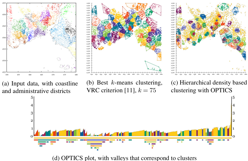
Fig. 1: Istanbul tweets data set

图 1: 伊斯坦布尔推文数据集

In Fig. 1 we introduce our running example. This data set contains 10,000 coordinates derived from real tweets in Istanbul. The raw coordinates can be seen in Fig. 1a, along with the coastline for illustration, and colored by administrative areas. Classic $k$ - means clustering can be seen in Fig.1b, with $k{=}75$ chosen by the Calinski-Harabasz criterion [11] (but this heuristic did not yield a clear “best” $k$ ). A hierarchical density-based clustering is shown in Fig.1c. This clustering does not partition all data points equally, but it emphasizes region of higher density, possibly even nested. Many of these regions correspond to neighborhood centers and shopping areas. Fig.1d shows the OPTICS plot for this clustering.

在图 1 中，我们介绍了我们的运行示例。该数据集包含从伊斯坦布尔的真实推文中提取的 10,000 个坐标。原始坐标可以在图 1a 中看到，同时为了说明，还绘制了海岸线，并按行政区域进行了着色。经典的 $k$ -均值聚类可以在图 1b 中看到，其中 $k{=}75$ 是通过 Calinski-Harabasz 准则 [11] 选择的（但该启发式方法并未产生一个明确的“最佳” $k$）。基于密度的层次聚类如图 1c 所示。这种聚类方法不会平等地分割所有数据点，但它强调了密度较高的区域，甚至可能是嵌套的。其中许多区域对应于社区中心和购物区。图 1d 显示了该聚类的 OPTICS 图。

The remainder of this article is structured as follows: In Section 2, we examine related work. Then we introduce the basics of OPTICS in Section 3 and cluster extraction from OPTICS plots in Section 3.3. Then we will discuss the extraction problem effecting all methods based solely on the OPTICS plot, as well as introducing a simple remedy for this problem in Section 4. Finally, we will demonstrate the differences on some example data sets in Section 5, and conclude the article in Section 6.

本文的其余部分结构如下：在第2节中，我们回顾了相关工作。然后在第3节中介绍了OPTICS的基础知识，并在第3.3节中讨论了从OPTICS图中提取聚类的方法。接着，我们将在第4节中讨论仅基于OPTICS图的所有方法所面临的提取问题，并介绍一个简单的解决方案。最后，我们将在第5节中通过一些示例数据集展示这些差异，并在第6节中总结本文。

2 Related Work

2 相关工作

DBSCAN [15] is the most widely known density based clustering method. In essence, the algorithm finds all connected components in a data set which are connected at a given density threshold given by a maximum distance $\varepsilon$ and the minimum number of points minPts contained within this radius. The approach has been generalized to allow other concepts of neighborhoods as well as other notions of what constitutes are cluster core point [28]. In [33], the authors revisit DBSCAN after 20 years, provide an abstract form, discuss the runtime in more detail, the algorithms limitations and provide some suggestions on parameter choices (in particular, how to recognize and avoid parameters). In OPTICS [6] the approach was modified to produce a hierarchy of clusters by keeping the minPts parameter, but varying the radius. Objects that satisfy the density requirement at a smaller radius connect earlier and thus form a lower level of the hierarchy. OPTICS however only produces an order of points, from which the clusters either need to be extracted using visual inspection [6], the $\xi$ method [6], using significant maxima [29] or inflexion points [8]. The relationship of OPTICS plots to d end ro grams (as known from hierarchical agglom erat ive clustering) has been discussed in [29].

DBSCAN [15] 是最广为人知的基于密度的聚类方法。本质上，该算法在数据集中找到所有在给定密度阈值下连接的连通分量，该阈值由最大距离 $\varepsilon$ 和该半径内包含的最小点数 minPts 给出。该方法已被推广，允许使用其他邻域概念以及构成簇核心点的其他定义 [28]。在 [33] 中，作者在 20 年后重新审视了 DBSCAN，提供了一个抽象形式，更详细地讨论了运行时间、算法的局限性，并提供了一些参数选择的建议（特别是如何识别和避免参数）。在 OPTICS [6] 中，该方法被修改为通过保持 minPts 参数但改变半径来生成聚类的层次结构。在较小半径下满足密度要求的对象会较早连接，从而形成层次结构的较低级别。然而，OPTICS 仅生成点的顺序，需要使用视觉检查 [6]、$\xi$ 方法 [6]、显著最大值 [29] 或拐点 [8] 从中提取聚类。OPTICS 图与树状图（如层次凝聚聚类中所知）的关系已在 [29] 中讨论。

Outside of clustering, the concepts of DBSCAN and OPTICS also were used for outlier detection algorithms such as the local outlier factor LOF [10] and the closely related OPTICS-OF outlier factor [9]. The concept of density-based clustering was also inspiration for the algorithms DenClue [20] and DenClue 2 [19], which employ gridbased strategies to discover modes in the density distribution. Both belong to the wider family of mode-seeking algorithms such as mean-shift clustering orignating in image analysis and statistical density estimation [17, 14]. The algorithm DeLiClu [3] employs an $\mathbf{R}^{*}$ -tree [7] to improve s cal ability, by performing a nearest-neighbor self-join on the tree. This can greatly reduce the number of distance computations, but increases the implementation complexity and makes the algorithm harder to optimize. It also removes the need to set the $\varepsilon$ parameter of OPTICS, as the join will automatically stop when everything is connected, without computing all pairwise distances.

在聚类之外，DBSCAN 和 OPTICS 的概念也被用于异常检测算法，例如局部异常因子 LOF [10] 和密切相关的 OPTICS-OF 异常因子 [9]。基于密度的聚类概念也启发了 DenClue [20] 和 DenClue 2 [19] 算法，这些算法采用基于网格的策略来发现密度分布中的模式。两者都属于更广泛的模式寻找算法家族，例如起源于图像分析和统计密度估计的均值漂移聚类 [17, 14]。算法 DeLiClu [3] 使用 $\mathbf{R}^{*}$ 树 [7] 来提高可扩展性，通过在树上执行最近邻自连接。这可以大大减少距离计算的数量，但增加了实现的复杂性，并使算法更难优化。它还消除了设置 OPTICS 的 $\varepsilon$ 参数的需要，因为当所有内容都连接时，连接将自动停止，而无需计算所有成对距离。

FastOPTICS [30, 31] approximates the results of OPTICS using 1-dimensional random projections, suitable for Euclidean space. The concepts of OPTICS were transferred to subspace clustering in the algorithms HiSC [2] and DiSH [1], for correlation clustering in HiCO [4], and to uncertain data in FOPTICS [22]. HDBSCAN* [12] is a revisited version of DBSCAN, where the concept of border points was removed, which yields a cleaner theoretical formulation of the algorithm, even closer connected to graph theory. In [13] the authors propose a general extraction strategy for hierarchical clusters that works well with HDBSCAN*, assuming that the hierarchy essentially corresponds to a minimum spanning tree. HDBSCAN* can be accelerated using dual-tree joins [26].

FastOPTICS [30, 31] 使用一维随机投影近似 OPTICS 的结果，适用于欧几里得空间。OPTICS 的概念被转移到子空间聚类算法 HiSC [2] 和 DiSH [1] 中，用于 HiCO [4] 中的相关聚类，以及 FOPTICS [22] 中的不确定数据。HDBSCAN* [12] 是 DBSCAN 的重新审视版本，其中移除了边界点的概念，这使得算法的理论表述更加清晰，更接近图论。在 [13] 中，作者提出了一种适用于 HDBSCAN* 的层次聚类提取策略，假设层次结构本质上对应于最小生成树。HDBSCAN* 可以使用双树连接 [26] 进行加速。

3 OPTICS Clustering

3 OPTICS 聚类

We will now first briefly review the core ideas of OPTICS clustering. The first idea is the notion of density reach ability, defining at which distance two neighbors are connected. Clusters are then connected components of this reach ability.

我们现在首先简要回顾一下 OPTICS 聚类的核心思想。第一个思想是密度可达性 (density reachability) 的概念，它定义了在什么距离下两个邻居是连接的。然后，聚类就是这种可达性的连接组件。

3.1 Reach ability Model of OPTICS

3.1 OPTICS 的可达性模型

OPTICS [6] uses the concept of “reach ability distance” for constructing clusters. This distance correspond y closely to the $\varepsilon$ radius parameter of DBSCAN, and can be seen as an inverse density estimate: all points within a cluster are “density connected” with at least this density. Reach ability is the maximum of two factors, the first being the actual distance of the two points, and the second being the core-distance of the origin point. In OPTICS [6], the core-distance was defined as

OPTICS [6] 使用“可达性距离”的概念来构建聚类。该距离与 DBSCAN 的 $\varepsilon$ 半径参数密切相关，可以视为逆密度估计：聚类内的所有点都“密度连接”，且至少具有此密度。可达性是两个因素的最大值，第一个是两点之间的实际距离，第二个是起始点的核心距离。在 OPTICS [6] 中，核心距离被定义为

where minPts -dist is the distance to the minPts nearest neighbor. In the following, we will omit the $\varepsilon_{\mathrm{max}}$ parameter and the associated UNDEFINED case from the original

其中 minPts -dist 是到 minPts 最近邻的距离。在下文中，我们将省略原始公式中的 $\varepsilon_{\mathrm{max}}$ 参数及其相关的 UNDEFINED 情况。

definitions for brevity.1 Furthermore, we can simply use infinity $\infty$ instead of a special UNDEFINED value. If $\varepsilon_{\mathrm{max}}$ is chosen large enough, this case does not occur, and we can substitute minPts -dist for the core-distance.

为了简洁起见，我们省略了定义。此外，我们可以简单地使用无穷大 $\infty$ 来代替特殊的 UNDEFINED 值。如果 $\varepsilon_{\mathrm{max}}$ 选择得足够大，这种情况就不会发生，我们可以用 minPts -dist 代替核心距离。

We can then define the reach ability of a point $p$ from a point $o$ as:2

然后我们可以将点 $p$ 从点 $o$ 的可达性定义为：2

Reach ability, while originally called “reach ability distance” is not a distance as defined in mathematics, because it is not symmetric. This asymmetry is often causing confusion, and we thus will only refer to it simply as “reach ability” here. Intuitively, this value is the minimum distance threshold $\varepsilon$ that we need to choose, to make $p$ density-reachable from $o$ and thus part of the same DBSCAN cluster. OPTICS is based on the same idea of clusters being connected components based on a reach ability threshold.

可达性（Reachability），最初被称为“可达性距离”，并不是数学上定义的距离，因为它不具备对称性。这种不对称性常常引起混淆，因此我们在这里仅简称为“可达性”。直观上，这个值是我们需要选择的最小距离阈值 $\varepsilon$，以使 $p$ 从 $o$ 密度可达，从而成为同一 DBSCAN 聚类的一部分。OPTICS 基于相同的聚类思想，即聚类是基于可达性阈值的连通分量。

The use of core distances prevents (for large enough minPts) the undesirable chaining effect known as “single-link effect” that affects hierarchical clustering, in particular on noisy data. For practical purposes, minPts must thus be chosen not too small, but values such as minPts $=5$ may be sufficient for small 2-dimensional data sets with little noise. The suggestions in [33] for choosing minPts in DBSCAN may be applicable.

核心距离的使用防止了（对于足够大的minPts）影响层次聚类的“单链效应”这一不良连锁反应，特别是在噪声数据上。因此，在实际应用中，minPts的选择不宜过小，但对于噪声较少的小型二维数据集，minPts $=5$ 可能已经足够。文献 [33] 中关于在DBSCAN中选择minPts的建议可能适用。

3.2 Algorithmic Aspects of OPTICS

3.2 OPTICS 的算法方面

The OPTICS agorithm is an efficient algorithm to approximate the density clustering structure given by the reach ability distance introduced above. It uses a greedy approach to find dense areas: it always processes the point with the currently lowest known reachability next (intuitively, the point with the highest expected density), removes it from the candidates and adds it to the output list, then updates the reach ability of its yet un processed neighbors if (and only if) it decreased.

OPTICS算法是一种高效的算法，用于近似上述引入的可达性距离给出的密度聚类结构。它采用贪婪的方法来寻找密集区域：总是处理当前已知可达性最低的点（直观上，预期密度最高的点），将其从候选点中移除并添加到输出列表中，然后更新其尚未处理的邻居的可达性（当且仅当可达性降低时）。

The output of OPTICS is an ordering of the database along with the reach ability of each object, but not clusters in the traditional sense of data partitions. Instead, different visual and automatic methods can be used to extract clusters from this order. The cluster order is not fully deterministic because points with the same distance may be processed in any order. Thus, different runs may yield different results that nevertheless correspond to a highly similar cluster structure.

OPTICS 的输出是数据库的排序以及每个对象的可达性，而不是传统意义上的数据分区集群。相反，可以使用不同的视觉和自动方法从此排序中提取集群。集群顺序并不完全确定，因为具有相同距离的点可以按任何顺序处理。因此，不同的运行可能会产生不同的结果，但这些结果仍然对应于高度相似的集群结构。

A key design aspect of the OPTICS algorithm is its efficiency $i f$ the database can accelerate radius queries. If the database can answer such queries for the given data set, distance function, and radius $\varepsilon_{\mathrm{max}}$ within $\log n$ time on average, then the run-time of OPTICS can be $n\log n$ instead of $O(n^{2})$ , making it suitable for large data sets.3 For too large radius $\varepsilon_{\mathrm{max}}$ , or “malicious” data sets, such run-times can usually not be guaranteed (c.f., [33]), so the worst-case run-time supposedly remains $O(n^{2})$ . In many practical applications, speedups of this magnitude can be observed empirically with indexes such as the k-d-tree and $\mathbf{R}^{*}$ -tree [7].

OPTICS 算法的一个关键设计方面是其效率，如果数据库能够加速半径查询。如果数据库能够在平均 $\log n$ 时间内回答给定数据集、距离函数和半径 $\varepsilon_{\mathrm{max}}$ 的此类查询，那么 OPTICS 的运行时间可以是 $n\log n$ 而不是 $O(n^{2})$，从而使其适用于大数据集。对于过大的半径 $\varepsilon_{\mathrm{max}}$ 或“恶意”数据集，通常无法保证这样的运行时间（参见 [33]），因此最坏情况下的运行时间可能仍然是 $O(n^{2})$。在许多实际应用中，使用诸如 k-d 树和 $\mathbf{R}^{*}$ 树 [7] 等索引可以经验性地观察到这种速度提升。

OPTICS uses a priority queue for processing points. Initially the queue is empty, and if a maximum distance $\varepsilon_{\mathrm{max}}$ is used, it may become empty again. If empty, an un processed point is chosen at random with a reach ability of $\infty$ . OPTICS polls one point $o$ at a time from this priority queue, adds it to the cluster order with its current reach ability, marks it as visited, and searches its neighborhood: For every neighbor $p$ of $o$ that has not yet been visited, reach ability $(p\leftarrow o)$ is computed, and the priority queue is updated, unless it already contains a better reach ability for $p$ .

OPTICS 使用优先队列处理点。初始时队列为空，如果使用了最大距离 $\varepsilon_{\mathrm{max}}$，队列可能会再次变为空。如果队列为空，则随机选择一个未处理的点，其可达性为 $\infty$。OPTICS 从该优先队列中每次轮询一个点 $o$，将其当前可达性添加到聚类顺序中，标记为已访问，并搜索其邻域：对于 $o$ 的每个尚未访问的邻居 $p$，计算可达性 $(p\leftarrow o)$，并更新优先队列，除非队列中已经包含 $p$ 的更好可达性。

The approach used by OPTICS bears similarities with Prim’s algorithm [27] for computing the minimum spanning tree; except that for efficiency OPTICS only considers edges with a maximum length of $\varepsilon_{\mathrm{max}}$ ; and the output is a linear order instead of a spanning tree. Intuitively, OPTICS builds the cluster order by always adding the point next which is best reachable from all previous points (and drawing one at random, if no point is reachable or there is no previous point).

OPTICS 使用的方法与 Prim 算法 [27] 在计算最小生成树时的方法有相似之处；不同之处在于，为了提高效率，OPTICS 只考虑最大长度为 $\varepsilon_{\mathrm{max}}$ 的边；并且输出是一个线性顺序，而不是生成树。直观上，OPTICS 通过始终添加从所有先前点中最佳可达的下一个点来构建聚类顺序（如果没有点可达或没有先前的点，则随机选择一个点）。

3.3 Cluster Extraction from OPTICS Plots

3.3 从 OPTICS 图中提取聚类

Density-based clusters correspond to “valleys” in OPTICS plots as seen in Fig. 1d, but the formal definition of a valley turns out to be more difficult than expected.

基于密度的簇对应于 OPTICS 图中的“谷”，如图 1d 所示，但谷的形式定义比预期的要困难。

OPTICS [6] defined the notion of $\xi$ -steep points if the reach ability of two successive points in the cluster order differs by a factor of more than $1{-}\xi$ . Downward steep points are candidates for the beginning of a cluster, and upward steep points are candidates for the end. The exact definitions of $\xi$ -clusters involves handling of additional constraints, such as ensuring a minimum cluster size and taking the minimum in-between value into account for inferring the hierarchical structure. Details on this can be found in [6].

OPTICS [6] 定义了 $\xi$ -steep 点的概念，如果簇顺序中两个连续点的可达性相差超过 $1{-}\xi$ 的因子。向下陡峭点是簇开始的候选点，而向上陡峭点是簇结束的候选点。$\xi$ -簇的精确定义涉及处理额外的约束，例如确保最小簇大小，并在推断层次结构时考虑中间的最小值。有关此内容的详细信息可以在 [6] 中找到。

This extraction method operates only on the OPTICS plot only, not on the original data: it identifies sub sequences that exhibit a steep gradient, and then selects the corresponding sub sequence of the cluster order. It works as desired, and often would select those areas a human expert would select base on visual inspection of the OPTICS plot.

这种提取方法仅作用于OPTICS图，而非原始数据：它识别出具有陡峭梯度的子序列，然后选择聚类顺序中对应的子序列。该方法按预期工作，通常会选择出人类专家通过视觉检查OPTICS图所选中的区域。

When running this algorithm on larger data sets, certain artifacts have been observed when inspecting the cluster in detail. This becomes most obvious when drawing the convex hulls of cluster of geographical points, as seen in Fig. 2a for Tweet locations in the Bosporus region (Fig. 2c and 2d are close-ups; lines are the convex hulls of the cluster points): some clusters have a spike extending from them that does not appear to be correct. Closer inspection revealed that these are always the last few objects within a cluster, and this problem can be provoked on a much smaller data set.

在更大的数据集上运行此算法时，详细检查集群时会观察到某些伪影。这在绘制地理点集群的凸包时最为明显，如图 2a 中博斯普鲁斯地区的推文位置所示（图 2c 和 2d 是特写；线条是集群点的凸包）：一些集群有一个从它们延伸出来的尖峰，这似乎不正确。更仔细的检查表明，这些总是集群中的最后几个对象，这个问题可以在更小的数据集上被引发。

4 Using Predecessor Information for Improved Cluster Extraction

4 利用前驱信息改进集群提取

The implementation of OPTICS in ELKI [5] includes additional information in the data structures, useful for visualizing the clustering process of OPTICS: it not only tracks the reach ability distance, but also the predecessor that had the smallest reach ability. This was added to ELKI for the DiSH algorithm [1], an OPTICS variant for finding subspace cluster hierarchies. While DiSH used this information to compare the “subspace preference” of a point to its predecessor, it turned out that this is exactly the information needed for resolving ambiguity of wheter a point at the end of a valley still belongs to

ELKI [5] 中 OPTICS 的实现包含了数据结构中的额外信息，这些信息对于可视化 OPTICS 的聚类过程非常有用：它不仅跟踪可达距离，还跟踪具有最小可达距离的前驱节点。这一功能是为 DiSH 算法 [1] 添加到 ELKI 中的，DiSH 是 OPTICS 的一个变体，用于寻找子空间聚类层次结构。虽然 DiSH 使用这些信息来比较点的“子空间偏好”与其前驱节点，但事实证明，这正是解决山谷末端点是否仍属于某个簇的歧义所需的信息。

Fig. 2: OPTICS without and with the proposed filtering

图 2: 未使用和使用所提出过滤方法的 OPTICS

Algorithm 2: Cluster refinement algorithm, to post process each cluster $(s,e)$ .

算法 2: 聚类优化算法，用于后处理每个聚类 $(s,e)$。

the cluster or not: if its predecessor is included in the cluster then the ambiguous point is also part of the cluster, but if the predecessor is in a parent cluster, the point should be part of the parent (or a subsequent cluster in the plot).

该点是否属于该簇：如果其前驱点包含在该簇中，则模糊点也是该簇的一部分；但如果前驱点位于父簇中，则该点应属于父簇（或图中的后续簇）。

Algorithm 2 gives the pseudocode of this surprisingly simple refinement algorithm, which can be integrated easily into the $\xi$ cluster extraction or other methods for extracting clusters from OPTICS plots. (The artifact is not specific to $\xi$ clusters, but these artifacts will occur in any method based on valleys in the cluster order.) The predecessor of the last (by cluster order) element in the cluster is searched in the cluster. If it is found, the algorithm terminates, but if the predecessor is not found, then the last element is discarded and the algorithm continues. Because of the priority heap used in OPTICS, all points with a reach ability less than the first point must have their predecessor in the cluster, so most points will cause successful termination. The necessary predecessor information can trivially be gathered while computing the OPTICS plot, and needs only $O(n)$ additional memory for storing the predecessors. Since we only have to look at a few elements at the end of each cluster, the runtime impact of this refinement is negligible compared to the cost of finding the neighbors.

算法 2 给出了这个出奇简单的优化算法的伪代码，该算法可以轻松集成到 $\xi$ 簇提取或其他从 OPTICS 图中提取簇的方法中。（该问题并非特定于 $\xi$ 簇，而是会出现在任何基于簇顺序中谷值的方法中。）在簇中搜索簇中最后一个（按簇顺序）元素的前驱。如果找到，算法终止；但如果未找到前驱，则丢弃最后一个元素并继续算法。由于 OPTICS 中使用了优先堆，所有可达性小于第一个点的点都必须在簇中有其前驱，因此大多数点都会导致成功终止。必要的前驱信息可以在计算 OPTICS 图时轻松收集，并且只需要 $O(n)$ 的额外内存来存储前驱。由于我们只需要查看每个簇末尾的几个元素，因此与查找邻居的成本相比，此优化的运行时影响可以忽略不计。

Fig. 3: Predecessors in the OPTICS plot.

图 3: OPTICS 图中的前驱节点。

Fig.2a visualizes the clusters without this algorithm, and Fig.2b after post-processing the clusters, with hardly visible differences. We indicate two (but not all) differences with arrows, and show these regions in more detail in Fig.2c and Fig.2d.

图 2a 展示了未使用该算法的聚类结果，图 2b 展示了经过后处理的聚类结果，两者几乎没有可见的差异。我们用箭头标出了两处（但并非全部）差异，并在图 2c 和图 2d 中更详细地展示了这些区域。

4.1 Theoretical Support for this Correction

4.1 该修正的理论支持

This correction technique is well supported by theory if we realize that the OPTICS plot is a linearized version of a spanning tree. If there exist multiple subtrees in the data, only one subtree can immediately follow in the OPTICS cluster order. After the first subtree, there will be some object which is the first of the next subtree. This object will necessarily have a higher reach ability than the first object of the first subtree (because of the priority queue). The converse is, however, not true, and we cannot rely on the reach ability alone. Instead, we need to consider the predecessor of the point.

如果我们意识到 OPTICS 图是生成树的线性化版本，那么这种校正技术在理论上是得到充分支持的。如果数据中存在多个子树，在 OPTICS 聚类顺序中，只有一个子树可以立即跟随。在第一个子树之后，会有一些对象是下一个子树的第一个对象。由于优先队列的存在，这个对象的可达性必然高于第一个子树的第一个对象。然而，反之则不成立，我们不能仅依赖可达性。相反，我们需要考虑该点的前驱。

Fig. 3 illustrates this principle. Points $\mathrm{^C}$ to I consitute a valley. But because the predecessor of I is B, and B is not part of the valley, it is not part of the cluster (the reach ability in the plot is reach ability $(I\leftarrow B)$ , and the reach ability of $I$ from any point between $B$ and $I$ is at least as much).

图 3 展示了这一原理。点 $\mathrm{^C}$ 到 I 构成了一个谷。但由于 I 的前驱是 B，而 B 不是谷的一部分，因此它不属于该簇（图中的可达性是 $(I\leftarrow B)$ ，并且从 $B$ 到 $I$ 之间的任何点到 $I$ 的可达性至少相同）。

Line 2 is a simple shortcut to avoid having to search the predecessor: When the point $s$ was added to the cluster order, it must have been the point with minimum reach ability (because of the priority queue). If $r(s)>r(e)$ , this implies that some predecessor of $e$ in the cluster order between $s$ and $e$ must have caused the reach ability of $e$ to decrease to this value $r(e)$ , and therefore this predecessor must be in the cluster. Note that for $r(s)\leq r(e)$ it is no longer guaranteed that $r(e)$ decreased after $s$ was added. In such cases, we employ the linear search in Line 3. We could avoid this search by storing the cluster order position of each element with additional $O(n)$ memory, but the search has very low constant factors, and is not invoked very often.

第2行是一个简单的快捷方式，用于避免搜索前驱点：当点 $s$ 被添加到聚类顺序中时，它必须是最小可达性点（因为优先级队列）。如果 $r(s)>r(e)$ ，这意味着在聚类顺序中 $s$ 和 $e$ 之间的某个前驱点必须导致 $e$ 的可达性降低到这个值 $r(e)$ ，因此这个前驱点必须在聚类中。注意，对于 $r(s)\leq r(e)$ ，不再保证 $r(e)$ 在 $s$ 被添加后降低。在这种情况下，我们在第3行使用线性搜索。我们可以通过存储每个元素的聚类顺序位置来避免这种搜索，但这需要额外的 $O(n)$ 内存，而搜索的常数因子非常低，并且不经常被调用。

While the proposed technique is an easy and effective modification of the existing cluster extraction techniques—and should be integrated to improve the results—it raises the question whether the linear iz ation of the spanning tree into the cluster order is appropriate in the first place. Instead, it may be reasonable to use a spanning directly instead of the processing order used by OPTICS. In fact, the recently proposed method HDBSCAN does exactly this: constructing a density based spanning tree of the data, and extracting clusters from this tree; unfortunately at the cost of increasing the complexity of the published algorithm to $O(n^{2})$ .

虽然所提出的技术是对现有聚类提取技术的一种简单而有效的修改——并且应该被整合以提高结果——但它首先提出了一个问题：将生成树的线性化转换为聚类顺序是否合适。相反，直接使用生成树而不是 OPTICS 使用的处理顺序可能是合理的。事实上，最近提出的方法 HDBSCAN 正是这样做的：构建基于密度的数据生成树，并从该树中提取聚类；但不幸的是，这增加了已发布算法的复杂度至 $O(n^{2})$。

The observation that OPTICS plots relate to d end ro grams is not completely new: In [29], the authors discuss how to convert an OPTICS cluster order into a dendrogram, or a dendrogram into a cluster order, but without realizing the role of the predecessor, and how this can be used here. And while OPTICS plots are a key contribution of the method, the roots of this visualization can be traced back to Ward [35], who used arrows of different length to indicate the clustering structure. Other early examples include skyline plots [36], the diagrams used by Johnson [21], and the “linear representations” of clusters in the book by Hartigan [18]. Icicle plots [23] closely resemble the OPTICS plot, but the main contribution claimed is to use the object labels for printing instead of blocks. These early methods will only scale to a few objects, as they usually require two characters or lines per object. The authors argue that these plots are easier to read off than the d end ro grams more commonly used with hierarchical clustering. We believe we are the first to point out the close relationship between these icicle/skyscraper plots and OPTICS reach ability plots. It is worth noting that the older plots plotted the separation distance inbetween of two points, whereas OPTICS reach ability plots use the reachability distance of a point. In fact, the reach ability is better interpreted as the separation from the points’ predecessor(s), i.e., the cophenetic distance [34].

OPTICS 图与树状图的关系并非全新发现：在 [29] 中，作者讨论了如何将 OPTICS 聚类顺序转换为树状图，或将树状图转换为聚类顺序，但未意识到前驱的作用及其在此处的应用。尽管 OPTICS 图是该方法的核心贡献，但这种可视化的根源可追溯至 Ward [35]，他使用不同长度的箭头来表示聚类结构。其他早期例子包括天际线图 [36]、Johnson [21] 使用的图表，以及 Hartigan [18] 书中提到的“线性表示”聚类。冰柱图 [23] 与 OPTICS 图极为相似，但其主要贡献在于使用对象标签而非方块进行打印。这些早期方法仅适用于少量对象，因为通常每个对象需要两个字符或行。作者认为这些图比层次聚类中更常用的树状图更易阅读。我们认为我们是第一个指出这些冰柱/摩天楼图与 OPTICS 可达性图之间紧密关系的人。值得注意的是，旧图绘制的是两点之间的分离距离，而 OPTICS 可达性图使用点的可达性距离。实际上，可达性更应被解释为点与其前驱的分离距离，即共表型距离 [34]。

So while we should rather define OPTICS clusters as subtrees of the implicit spanning tree, rather than further using the current visual approach based on the cluster order and plot. But as mentioned before this ultimately leads to the HDBSCAN* [12] algorithm. In this paper, we rather discuss a small modification to OPTICS cluster extraction, that can easily be added to an existing implementation.

因此，我们应该将 OPTICS 聚类定义为隐式生成树的子树，而不是继续使用基于聚类顺序和图表的当前可视化方法。但如前所述，这最终导致了 HDBSCAN* [12] 算法的出现。在本文中，我们讨论了对 OPTICS 聚类提取的一个小修改，该修改可以轻松地添加到现有实现中。

5 Experiments

5 实验

We continue with the running example using Tweets in Istanbul introduced in Section 3. Fig. 2 shows the clusters without and with the proposed modification. In Table 1 we show the change in density caused by our filtering approach. While it would be possible for a cluster to disappear because of filtering (if it shrinks below the minimum cluster size), this did not occur here. Out of 70 clusters (hierarchical, including the top level cluster containing everything), only 7 clusters were modified, and a total of 11 points were assigned to the parent cluster instead. With most evaluation measures such as the adjusted Rand index (ARI), normalized mutual information (NMI), but also most internal measures, this change would only make a negligible difference, as only $0.11%$ of points have changed the cluster assignment.

我们继续使用第3节中介绍的伊斯坦布尔推文作为运行示例。图2展示了未修改和修改后的聚类结果。表1展示了我们过滤方法导致的密度变化。虽然由于过滤可能导致一个聚类消失（如果它缩小到最小聚类大小以下），但在这里并未发生这种情况。在70个聚类中（层次聚类，包括包含所有内容的顶层聚类），只有7个聚类被修改，总共有11个点被分配到父聚类。对于大多数评估指标，如调整兰德指数（ARI）、归一化互信息（NMI），以及大多数内部指标，这种变化只会产生微不足道的差异，因为只有$0.11%$的点改变了聚类分配。

Therefore, we evaluate the change in cluster area instead. For each cluster, we compute the convex hull, and compute the polygon area using the Shoelace formula. As we can see in Table 1, removing a single mis assigned point reduced the area of the polygon up to $80%$ . For comparison, we give the maximum and the average area reduction possible by removing a single cluster member. As we can see, the filtered clusters are much less affected by random removal. We also include the four non-modified clusters with the largest possible area reduction as comparison. While we can see that while these have a larger area reduction than cluster $#49$ , they are also smaller, and we can thus expect the area to depend more on the individual points. This also shows in the larger area reduction when removing a random point. But most importantly, our approach is well supported by theory, as opposed to a heuristic threshold-based cluster pruning. Furthermore, cluster #51 is already unusually small, with just $0.077\mathrm{km^{2}}$ : the Sinan Erdem Dome, the tiny orange cluster embedded in the larger cluster (which is cluster $#50$ , corresponding to Ataköy, Bakırköy) in the bottom right of Fig.2c.

因此，我们评估了聚类区域的变化。对于每个聚类，我们计算凸包，并使用鞋带公式计算多边形面积。正如我们在表 1 中看到的，移除一个错误分配的点可以将多边形面积减少多达 $80%$。为了进行比较，我们给出了通过移除单个聚类成员可能实现的最大和平均面积减少量。正如我们所看到的，过滤后的聚类受随机移除的影响要小得多。我们还包括了四个未修改的聚类，这些聚类具有最大的可能面积减少量作为比较。虽然我们可以看到这些聚类的面积减少量比聚类 $#49$ 更大，但它们也更小，因此我们可以预期面积更依赖于单个点。这在移除随机点时的更大面积减少量中也得到了体现。但最重要的是，我们的方法得到了理论的支持，而不是基于启发式阈值的聚类修剪。此外，聚类 #51 已经异常小，仅为 $0.077\mathrm{km^{2}}$：Sinan Erdem Dome，嵌入在更大聚类中的微小橙色聚类（即聚类 $#50$，对应于 Ataköy, Bakırköy）位于图 2c 的右下角。

Table 1: Change in cluster area by removing points.

表 1: 移除点后的聚类区域变化

Clu.#	points	filtered	unfiltered
	before	change	area
#18	313	-4	3.09
#27	137	-1	0.79
#49	119	-1	1.23
#50	179	-1	2.23
#56	271	-1	7.43
#64	53	-2	1.04
#65	58	-1	1.27
#31	59	0
#43	94	0
#51	51	0
#68	81	0

6 Conclusions

6 结论

In this paper, we improve OPTICS clustering by storing the predecessor of each point, and taking this information into account during cluster extraction. The changes to the resulting clustering is small, usually just 0-2 samples per cluster. Because of this, this difference easily goes unnoticed when just looking at clustering evaluation measures such as the adjusted Rand index (ARI), or normalized mutual information (NMI). However because these points do not fit the resulting clusters well, they have a major impact on the volume of the cluster. This can easily be seen when using the convex hull on geographic data. The same effect however exists in other distances and in highdimensional data as well. The proposed improvement is well supported by theory, as it prunes points based on the spanning tree used implicitly by OPTICS. Because the necessary improvements require only $O(n)$ additional memory and neglibile run-time, they should be used by default, and have in an earlier variant already been integrated in the open-source ELKI [32] data mining framework since version 0.7.0 as well as the dbscan R package since version 1.0-0. This article explains the theoretical foundation of this beneficial filtering technique.

本文通过存储每个点的前驱节点，并在簇提取过程中考虑这一信息，改进了OPTICS聚类。由此产生的聚类变化很小，通常每个簇只有0-2个样本。因此，仅通过查看聚类评估指标（如调整兰德指数 (ARI) 或归一化互信息 (NMI)）时，这种差异很容易被忽视。然而，由于这些点与生成的簇不太匹配，它们对簇的体积有重大影响。在使用地理数据的凸包时，这一点很容易看出。然而，同样的效果也存在于其他距离和高维数据中。所提出的改进在理论上有很好的支持，因为它基于OPTICS隐式使用的生成树来修剪点。由于必要的改进只需要 $O(n)$ 的额外内存和可忽略的运行时间，因此应默认使用它们，并且早期版本已经集成到开源ELKI [32]数据挖掘框架（自0.7.0版本起）以及dbscan R包（自1.0-0版本起）。本文解释了这种有益过滤技术的理论基础。

Bibliography

参考文献